Multi-Dimensional Automatic Detection of Scanning Radar Images of Marine Targets Based on Radar PPInet

Abstract

Traditional radar target detection algorithms are mostly based on statistical theory. They have weak generalization capabilities for complex sea clutter environments and diverse target characteristics, and their detection performance would be significantly reduced. In this paper, the range-azimuth-frame information obtained by scanning radar is converted into plain position indicator (PPI) images, and a novel Radar-PPInet is proposed and used for marine target detection. The model includes CSPDarknet53, SPP, PANet, power non-maximum suppression (P-NMS), and multi-frame fusion section. The prediction frame coordinates, target category, and corresponding confidence are directly given through the feature extraction network. The network structure strengthens the receptive field and attention distribution structure, and further improves the efficiency of network training. P-NMS can effectively improve the problem of missed detection of multi-targets. Moreover, the false alarms caused by strong sea clutter are reduced by the multi-frame fusion, which is also a benefit for weak target detection. The verification using the X-band navigation radar PPI image dataset shows that compared with the traditional cell-average constant false alarm rate detector (CA-CFAR) and the two-stage Faster R-CNN algorithm, the proposed method significantly improved the detection probability by 15% and 10% under certain false alarm probability conditions, which is more suitable for various environment and target characteristics. Moreover, the computational burden is discussed showing that the Radar-PPInet detection model is significantly lower than the Faster R-CNN in terms of parameters and calculations.

1. Introduction

Radar is one of the main sensors for marine target detection, which can detect targets by emitting electromagnetic waves without being restricted by day and night, and can also penetrate clouds, rain, and fog [1]. In fact, the sea environment is complex and the marine targets are diverse, so the target’s returns are sometimes weak, which makes radar detection rather difficult [2,3]. Adaptive and robust detection of marine targets is the key technology, which has received widespread attention from researchers all over the world [4]. Specifically, there are two difficulties as follows. On the one hand, the environment is complex and changeable, and it is difficult to describe the clutter characteristics using specific distribution models [5], e.g., Rayleigh distribution, log-normal distribution, or K distribution. On the other hand, the target characteristics are complex and diverse as well [6], e.g., small size, stationary, moving, maneuvering, dense, etc. [7]. The improvement of radar’s target detection ability requires accurate realization of clutter suppression, target characteristic matching, and feature description [8]. Traditional statistical detection methods need to assume models, such as the distribution types and distribution characteristics of the background [4,5,6]. However, these methods are not accurately matched with the actual sea environment and target characteristics in case of different sea states. If radar returns do not match the preset model, the processing method will face serious performance degradation.

The traditional radar target detection methods can be mainly divided from the perspective of processing domains, e.g., time domain, frequency domain, and time-frequency (TF) domain, to improve the signal-to-noise/clutter ratio (SNR/SCR). The classic methods of time-domain processing include coherent or non-coherent accumulation and constant false-alarm rate (CFAR) detection [4,5]. However, they are usually intended for specific conditions, and it is difficult to ensure a high detection probability in the case of a dynamic and changing environment with non-Gaussian, non-stationary, and non-linear properties. The frequency domain processing methods include the moving target indicator (MTI) [9,10] and moving target detection (MTD) [11,12], which use Doppler information by Fourier transform. It is easy to distinguish moving targets from clutter using a Doppler filter, but this kind of method is affected by the target’s motion characteristics. In the case of variable speed and maneuvering targets, the Doppler spectrum is broadened and the energy accumulation is difficult [13,14]. Short-time Fourier transform (STFT) and short-time fractional FT (STFRFT) [7] are typical TF methods. However, the TF resolution of STFT is not satisfied and STFRFT needs transform angle searching to match the motion characteristics of the target, which makes it rather complex.

In order to deal with the above problems and challenges, radar needs to develop intelligent processing with self-learning, adapting, and self-optimizing capabilities. The development of artificial intelligence technology in recent years has provided technical support for the intelligent design of radar [15,16]. Artificial intelligence technology possesses the ability to simulate the memory, learning, and decision-making process through sample training. It is now widely used in vision systems, big data analysis, image interpretation, multi-task optimization, and other fields [17,18]. The concept of deep learning was first proposed by Hinton et al. [19]. Because it was the study of artificial neural networks, it was also called deep neural networks (DNNs). Later, it gradually developed into an important branch of machine learning, including the convolutional neural network (CNN) [20], recurrent neural network (RNN) [21], deep belief network (DBN) [22], generative adversarial network (GAN) [23,24], etc. It can automatically learn and extract the features of the signal or image, and realize tasks, such as intelligent recognition of speech information, detection, and segmentation of images. Recently, deep learning has been applied and developed in the field of radar, especially for intelligent detection and processing of high-resolution synthetic aperture radar (SAR) images [25].

As an important part of deep learning, CNN has achieved good results in the field of image target detection. Figure 1 is a context diagram of the development of CNN target detection algorithms since 2012. The lower part is the development of classical CNNs [19] from AlexNet to VGGNet, to GoogleNet, ResNet, and later DenseNet, MobileNet [26], etc. The upper part is the development of a detection algorithm based on CNN. The methods mainly include a two-stage detection algorithm and single-stage detection algorithm. The former is R-CNN, spatial pyramid pooling (SPP)-Net, Fast R-CNN, Faster R-CNN [27], FPN, Mask R-CNN [28], etc. A region suggestion generator is formed, where features are extracted, and a classifier is used to predict the category of the proposed area. The latter includes YOLO [29], SSD [30], etc., which directly makes classification and prediction for the objects in each position of the feature map. The intelligent algorithm of target detection based on CNN has realized improvement of the detection speed and accuracy, and has great advantages compared with traditional target detection algorithms.

Although deep learning-based methods have good capabilities for high-resolution SAR, ISAR, or time-frequency images, the performances in strong noise or a clutter background are not satisfactory. Moreover, most radars are narrow-band scanning radars, and the formed range-azimuth images are not high-resolution images [31]. Few studies have researched deep learning target detection for radar plain position indicator (PPI) images, especially marine radar. Therefore, there is an urgent need to design a radar image target detection method suitable for a complex sea clutter background. Recently, we carried out studies on radar image detection based on deep learning, and proposed classification of marine targets with micro-motion based on CNN [32], integrated network (INet) for clutter suppression and target detection [33], sea clutter suppression generative adversarial network (SCSGAN) [24] etc., using the radar range, azimuth, and time-frequency information to improve the detection performance. In this paper, a novel Radar-PPInet is designed for PPI image detection in complex scenarios (ocean, land, islands, etc.). The main work and contribution of this paper are summarized as follows:

(1)

An effective and efficient marine target detection network (Radar-PPInet) is proposed for scanning radar PPI images. It uses the multi-dimensional information, i.e., range-azimuth-interframe, and breaks through the limitations of traditional statistical detection methods, i.e., not limited by the assumptions of the environment model. It can adaptively learn the characteristics of the target and clutter and improve the generalization ability.

(2)

The proposed Radar-PPInet includes four contributions. Firstly, the prediction frame coordinates, target category, and corresponding confidence are directly given through the feature extraction network in Radar-PPInet. The network structure is lightened, and at the same time it shows good performance for the detection accuracy and speed. Secondly, the network structure strengthens the receptive field and the attention distribution structure. Through repeated use of the feature map extracted after convolution, that is, multiple up and down sampling and residual stacking are performed, which further strengthens the network training efficiency. Thirdly, the power non-maximum suppression (P-NMS) is designed to screen the final target detection frame, which can effectively improve the problem of missed detection of multi-targets. Lastly, a multi-frame information fusion strategy is proposed to further reduce false alarms, i.e., strong sea clutter, such as sea spikes.

The rest of the paper is organized as follows. The radar PPI images’ characterization and dataset construction is established in Section 2. Additionally, we introduce the principle of Radar-PPInet and present the detailed detection procedure. The effectiveness of the proposed method is demonstrated and validated by coastal and open sea radar images in Section 3. The performance comparison with CFAR and Faster R-CNN and computational burden are discussed in Section 4. Section 5 concludes the paper and presents the future research direction.

2. Materials and Methods

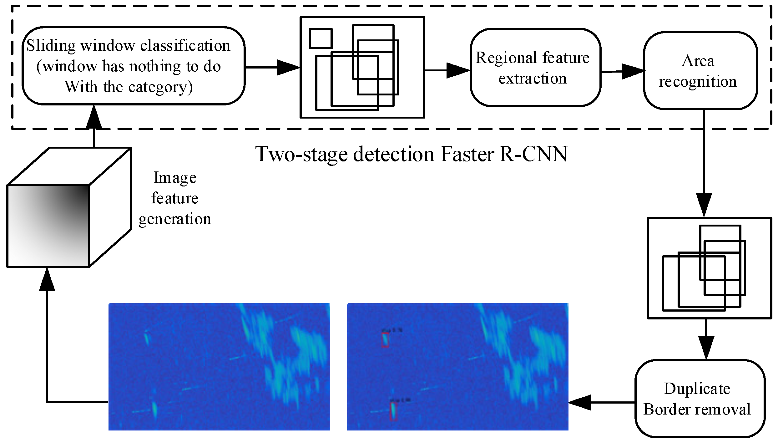
2.1. Radar PPI Image Target Detection Based on the Two-Stage Detection Algorithm Faster R-CNN

Faster R-CNN is the common deep learning target detection algorithm [3]. It includes three parts: shared CNN, region proposal network (RPN), and classification and regression network. The shared CNN can extract target features and input the extracted feature maps into the RPN and region of interest (ROI). The RPN completes the task of generating candidate frames, and inputs the generated candidate frames and the feature maps extracted by the shared CNN into the ROI. Finally, the classification and regression network realizes the final detection and classification. The RPN and classification and regression network improve the accuracy of classification and the regression candidate frame parameters by continuous iterative training. The radar PPI image detection flowchart via Faster R-CNN is shown in Figure 2. There are two points that should be explained in detail. (1) For each input picture, each layer of the neural network performs multi-core convolution on it, and each convolution kernel corresponds to a feature map generated after convolution, so multiple convolution kernels are convolved at the same time to form a feature map cube. (2) The sliding window has no fixed size; it is set according to the size of the image in the dataset.

The structure of the two-stage detection Faster R-CNN network is shown in Figure 3. It can be divided into four main parts: convolutional layers, RPN layer, ROI layer, and classification layer. Here, we show an example of an M × N image to illustrate the functions of the four layers in the network. The convolutional layer contains 13 convolutional layers, 13 fully connected layers, and 4 pooling layers. After convolution, fully connected pooled multi-layer CNN, it provides feature maps for the subsequent RPN and fully-connected layers. In the convolutional layer, all the convolution kernels’ size is 3, with compensation of 1 (equivalent to adding one pixel border to the image) and step size of 1, and all the pooling layer convolution kernels’ size is 2, with compensation of 0 and step size of 2. Therefore, the convolutional layer of the Faster R-CNN performs edge expansion processing on all convolutions (compensation is 1, i.e., the border of the image is filled with 0 before convolution). Then, the image becomes (M + 2) × (N + 2) after edge expansion processing. After the 3 × 3 convolution, the output of the image size can be obtained as M × N, achieving the goal of no information losses. Similarly, in the convolutional layer, the size of all the convolution kernels of the pooling layer is 2 with a step size of 2, and each matrix passing through M × N will become (M/2) × (N/2) in size. In summary, because the convolutional layer contains four pooling layers, the original image of the input M × N will become the size (M/16) × (N/16) after passing through the convolutional layer.

The feature map extracted by the convolutional layer is input to the RPN on one side and the ROI pooling layer on the other side. As shown in Figure 3. The region proposal network (RPN) is actually divided into two lines, where one is used to obtain positive and negative attributes through the softmax classification of the anchor frame, hereinafter referred to as the judgement branch, and the other is used to calculate the bounding box regression offset of the anchor frame, hereinafter referred to as the correction branch. The proposal layer integrates the positive attribute anchor box and the corresponding bounding box regression offset to obtain the feature map. At the same time, it can also filter out the feature map, which has an unreasonable size and is beyond the boundary. So far, the function of target positioning is completed.

The main function of the RPN is introduced. Before inputting the reshape and softmax, the RPN will mark anchors on the original image. The anchors are actually a set of matrices. Each row $\left(X_1,Y_1,X_2,Y_2\right)$ refers to the coordinates of the upper left corner, upper right corner, lower left corner, and lower right corner of the first anchor. The RPN is equipped with nine anchors for each point of the feature maps as the initial detection frame. The softmax in the judgement branch of the RPN determines the positive/negative attributes of the nine anchors of each point and stores the position information of the positive anchors. The function of the RPN correction branch is to make the positive anchors closer to the ground truth (GT). For the positive anchors, we generally use four-dimensional vectors (x, y, w, h) to represent the center point coordinates and width height of the anchors. The function of the correction branch mainly relies on the translation and scaling of the positive anchors. The positive anchor A = $\left(A_{\mathrm{x}},A_y,A_w,A_h\right)$ is set, the GT = $\left(G_x,G_y,G_w,G_h\right)$, and a certain change F satisfies:

$$F\left(A_{\mathrm{x}},A_y,A_w,A_h\right)=\left(G_x^{\prime },G_y^{\prime },G_w^{\prime },G_h^{\prime }\right)\approx \left(G_x,G_y,G_w,G_h\right)$$

(1)

Perform translation:

$$G_x^{\prime }=A_w\cdot d_x\left(A\right)+A_x,G_y^{\prime }=A_h\cdot d_y\left(A\right)+A_y.$$

(2)

Then perform zoom calculation:

$$G_w^{\prime }=A_w\cdot \exp \left(d_w\left(A\right)\right),G_h^{\prime }=A_h\cdot \exp \left(d_h\left(A\right)\right).$$

(3)

It is easy to obtain from (2) and (3) that the content that needs to be learned by the RPN correction branch network is the four transformations $d_x\left(A\right),d_y\left(A\right),d_w\left(A\right),d_h\left(A\right)$. In general, it can be considered that the difference between the positive anchors A and the GT is small, and the four transformations can be considered as linear transformations. It can be converted to a linear regression problem $Y=W\cdot X$. The input $X$ is the feature map extracted by the convolutional layer, which is defined as $\varphi$; the transformation amount between A and GT obtained by training is defined as $\left(t_x,t_y,t_w,t_h\right)$. Four transformations $d_x\left(A\right),d_y\left(A\right),d_w\left(A\right),d_h\left(A\right)$ are output. The objective function can be expressed as:

$$d_{\ast }\left(A\right)=W_{\ast }^{\mathrm{T}}\cdot \varphi \left(A\right)$$

(4)

where $d_{\ast }\left(A\right)$ is the obtained predicted value, $\varphi \left(A\right)$ is the feature vector composed of the feature map of the corresponding positive anchors, $W_{\ast }$ is the parameter to be learned, ${(\cdot )}^{\mathrm{T}}$ and $\ast$ represent the transpose operation and the four transformed coordinates $x,y,w,h$, respectively. In order to minimize the difference between the predicted transformation amount $d_{\ast }\left(A\right)$ and the real transformation amount $t_{\ast }$, the l1 loss function is calculated as:

$$Loss={\displaystyle \sum _i^N|t_{\ast }^i-W_{\ast }^{\mathrm{T}}\cdot \varphi \left(A^i\right)|}$$

(5)

The optimization goal is:

$$\stackrel{\wedge }{W_{*}}=\underset{W_{*}}{\mathrm{argmin}}{\displaystyle \sum _i^n|t_{\ast }^i-W_{\ast }^{\mathrm{T}}\cdot \varphi \left(A^i\right)|}+\lambda \Vert W_{\ast }\Vert$$

(6)

where λ is a regulation parameter. The relationship between the amount of translation $\left(t_x,t_y\right)$ and the scale factor $\left(t_w,t_h\right)$ of the positive anchor and ground truth is as follows:

$$t_x=\left(x-x_a\right)/w_a,t_{\mathrm{y}}=\left(y-y_a\right)/h_a,t_w=\log \left(w/w_a\right),t_h=\log \left(h/h_a\right)$$

(7)

where $w_a$ and $h_a$ are the width and height of GT’s frame.

In summary, in the case of input $\varphi$, the network output and the supervision signal $\left(t_x,t_y,t_w,t_h\right)$ should be as close as possible. Positive anchors, and their transformation amount d_x(A), d_y(A), d_w(A), d_h(A) and im info, are input into the proposal layer and then processed in the following order:

(1)

Generate anchors;

(2)

Do regression on all anchors using d_x(A), d_y(A), d_w(A), d_h(A);

(3)

Sort the anchors from large to small according to the input positive softmax scores and extract the positive anchors after the correction position;

(4)

Limit the positive anchors beyond the image boundary as the image boundary to prevent the proposal exceeding the image boundary;

(5)

Remove the very small positive anchors;

(6)

Perform non-maximum suppression (NMS) on the remaining positive anchors;

(7)

Output the proposals.

The size and shape of the proposal output by the RPN network are different. The ROI pooling layer uses the spatial scale parameter to map the proposal back to the feature map scale of (M/16) × (N/16), and then the feature map area corresponding to each proposal is divided into pooled_w × pooled_h grids. Finally, max pooling is performed on each grid. Then, proposals with different sizes are output with a fixed size pooled_w × pooled_h.

After the classification layer obtains the feature map with a fixed size, the attributes of each proposal in the preset category are calculated by the fully connected layer and softmax, and the cls_prob probability vector is output. In addition, the bounding box regression is used again to obtain the position offset bbox_pred of each proposal, for more accurate target positive anchors.

2.2. Radar PPI Image Target Detection Based on Radar-PPInet

The marine target in radar PPI images is a small-scale target relative to the overall PPI image, and Faster R-CNN usually faces the problem of a high false alarm rate and missing target, especially under a complex sea background. In this paper, the single-stage detection YOLO network is modified and improved for a novel network named Radar-PPInet, which can better adapt to the target detection of radar PPI images under the background of strong sea clutter and multiple marine targets.

2.2.1. Introduction to the Traditional YOLO Model

The classic single-stage detection algorithm the YOLO network [34] is shown in Figure 4. Its structure can be divided into two main parts, i.e., the convolutional layer (conv layer) andfully connected layer (FC). C.R. means convolution operation. It is supposed that the input image size is 448 × 448, which is divided into 7 × 7 grids. During training, GT is used to calculate the center of the object to fall into a certain grid, and the grid is used to detect the object. Each grid will predict two bounding boxes and their corresponding confidence scores, which can reflect the confidence of an object being contained in the box and the accuracy of the bounding box. Each bounding box contains the prediction box (x, y, w, h) and confidence scores. (x, y) represents the position of the prediction box center relative to the boundary, and (w, h) represents the ratio of the width and height of the prediction box to the original image. The confidence scores are the intersection over union (IOU) of the bounding box and GT. The position of the bounding box is the result of the network. After determining the initial value of the model weight and the input image, the position of the bounding box is determined by model calculation, and the GT is used in the training process to adjust the predicted position of the bounding box.

2.2.2. The Structure of Novel Radar-PPInet

Radar-PPInet mainly includes five parts: CSPDarknet53, SPP, PANet, P-NMS, and the multi-frame fusion section, as shown in Figure 5.

Assuming that the radar image input to the backbone feature extraction network is 416 × 416 × 3, firstly a convolution normalization and an activation function are performed, and the feature layer is obtained (416 × 416 × 32). Using the Mish activation function, the difference can be kept at a negative value, so as to stabilize the output gradient flow, feedback, and update each sensory neuron. Compared with the LeakyReLU function, the Mish function has stronger computing ability and can accommodate more weight calculations:

$$\mathrm{Mish}=x\cdot \tanh \left(\ln \left(1+{\mathrm{e}}^x\right)\right)$$

(8)

where $\tanh i=\frac{{\mathrm{e}}^i-{\mathrm{e}}^{-i}}{{\mathrm{e}}^i+{\mathrm{e}}^{-i}}$ is the hyperbolic tangent function.

Then, the feature layer is compressed through the residual block (Resblock) body residual network five times, and the CSPNet structure is mainly used. As shown in Figure 6, the stacking of multiple computing layers can realize the processing and computation of input information. The hierarchical expression of the input information by the output of the upper layer as the input of the next layer is the basic idea of deep learning. During the stacking process of the CSPNet, the left branch will have a very large residual edge. After the feature layer is extracted from the residual stack of the right network, the output connection is made with the left branch. Then, three effective feature layers are obtained with a size of 52 × 52 × 256, 26 × 26 × 512, and 13 × 13 × 1024, respectively.

The effective feature layer of 13 × 13 × 1024 is input into the SPP network after 3 convolution operations, and the input feature layer is pooled with different sizes of pooling kernels, i.e., 5 × 5, 9 × 9, and 13 × 13, respectively. The output of the SPP network is convolved and upsampled, stacked, and convolved 5 times with the output of the 26 × 26 × 512 feature layer convolution, and the output is named A. A and the output of 52 × 52 × 256 feature layer convolution are stacked and convolved 5 times, and the output is named B. B is downsampled, convolved, and stacked with A 5 times, and the output is named C. After C is downsampled, it is stacked and convolved 5 times with the SPP network output, and the result is named D. B, C, and D are the outputs of the Radar-PPInet head. The Radar-PPInet head is essentially the prediction result of the network, which is the basis for the following detection bounding box obtained after the feature layer processing.

The multiple bounding boxes predicted by the three Radar-PPInet heads are continuously input to the P-NMS layer to screen out the final target detection frame. The novel P-NMS can improve the problem of missed detection of multiple targets. In the actual marine target detection scene, multiple targets are often encountered. In this case, it is more likely to cause missed detection, which greatly limits the generalization ability and detection accuracy. The core idea of NMS is to remove all candidate frames that overlap with the optimal candidate frame. The formula is as follows [35]:

$$s_i=\{\begin{array}{ll}{s}_i,& \mathrm{IOU}\left(M,b_i\right)<N_t\\ 0,& \mathrm{IOU}\left(M,b_i\right)\ge N_t\end{array}$$

(9)

where s_i is the score of the i-th candidate box, M is the current highest-scoring box, b_i is the to-be-processed box, N_t is the detection threshold, and IOU is the ratio of the intersection and union between the prediction box and the labeled box.

However, in actual situations, the candidate frames of multiple marine targets may overlap, and the NMS algorithm suppresses all candidate frames with overlap higher than a certain threshold, which may cause the missing detection of individual targets. The proposed P-NMS is suitable for the detection of multiple targets with a certain degree of overlap in candidate frames, which is defined as follows:

$$s_i=\{\begin{array}{ll}{s}_i,& \mathrm{IOU}\left(M,b_i\right)<N_t\\ s_i{\left(\mathrm{IOU}\left(M,b_i\right)\right)}^2,& \mathrm{IOU}\left(M,b_i\right)\ge N_t\end{array}$$

(10)

2.2.3. Sea Clutter False Alarms Reduction via Multi-Frame Fusion

In order to further reduce false alarms, pre-training can be used to further improve the detection probability. Pre-training refers to training the model first, using the network parameters of the optimal model obtained after testing as the initial parameters of the network during real training, and then training the model based on the pre-training network to further optimize the network model parameters. Ground clutter and sea clutter are the main reasons for the high false alarms. After Radar-PPInet, the sea clutter can be further suppressed by fusion of the multi-frame PPI image detection results. Following the idea of the target track initiation algorithm in radar data processing, i.e., logic method, multi-frame image fusion is employed to reduce false alarms. The specific implementation is as follows in Figure 7.

The sequence ($z_1,z_2,\cdots ,z_i,\cdots ,z_n$) represents the Radar PPInet detection results with n radar scans. If there is a target detected in the correlation gate during the ith scan, the element $z_i=1$; otherwise, it is 0. When the number of detections k in a certain area of n scans reaches or is more than a certain value m, i.e., $k\ge m$, it is regarded as a target; otherwise, it is judged as a sea clutter false alarm. This is called the m/n logic criterion. The m/n value setting needs to comprehensively consider the sea state, target movement speed, and system processing capacity. It is appropriate to select $1/2<m/n<1$ within multiple scans. For example, for low sea states, the sea clutter is weak and false alarms are not likely to occur, and the number of n can be smaller (m/n = 2/3); for high sea conditions, the sea clutter is stronger and false alarms are likely to occur. The number of n can be larger (m/n = 3/5); for marine maneuvering and fast-moving targets, the gate can be estimated by extrapolating the approximate speed.

2.2.4. The PPI Image Detection Procedure via Radar-PPInet

The flowchart of the radar image marine target detection algorithm via Radar-PPInet is shown in Figure 8.

The detailed procedure is shown as follows:

(1)

Scanning radar echo data preprocessing, such as sensitivity-time control (STC), in order to suppress the short-range strong clutter. This step is generally used for a high sea state environment.

(2)

Collect and record radar echo data, and convert the echo data into PPI images.

(3)

Construct a marine target image dataset. Crop PPI images, and use AIS and other information to mark and label marine targets.

(4)

Establish the radar image target detection network (Radar-PPInet), which mainly includes CSPDarknet53, SPP, PANet, PNMS, and multi-frame fusion.

(5)

Train and optimize the model. The PPI images dataset is input to the Radar-PPInet model for iterative training, and the initial training parameters of the model are adjusted and optimized to obtain the optimal network parameters;

(6)

Generate images from real-time radar echoes, input them into the trained Radar-PPInet target detection model for testing, and obtain target detection results.

3. Experimental Results and Analysis

In this section, X-band marine radar PPI images are used to verify the performance of the proposed algorithm. Moreover, the detection performance is compared with two-dimensional (2-D) cell-average (CA)-CFAR and Faster R-CNN.

3.1. Marine Radar PPI Images Datasets

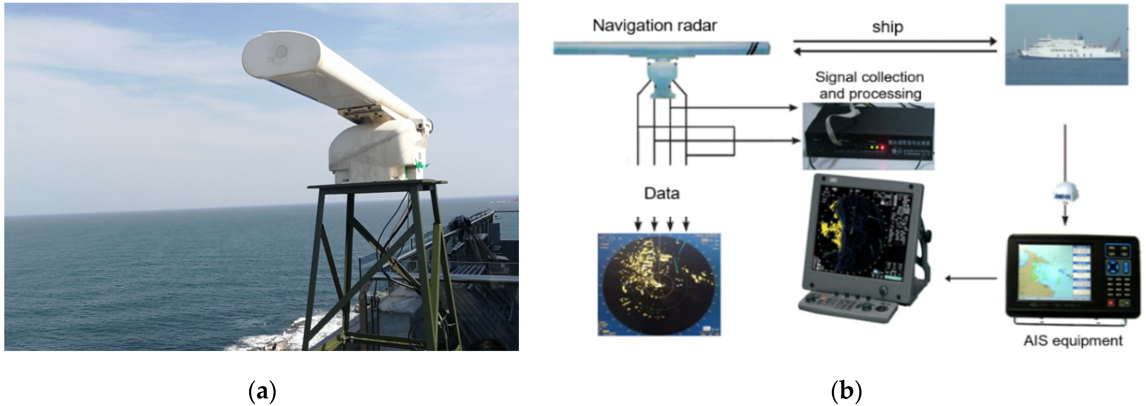
3.1.1. Navigation Radar Data Acquisition

The radar PPI image is the radar display on the terminal, which mainly displays the original image of the target’s echo, including the target’s distance, azimuth, elevation, altitude, and position. The dataset used in this paper is collected by an X-band solid-state navigation radar, which is mainly used in ship navigation and coastal surveillance scenarios. The radar uses a solid-state power amplifier with a transmission time range of 40 ns–100 µs and pulse compression method, which can not only effectively reduce the radar radiation power, but also improve the range resolution [36]. The technical parameters of the X-band solid-state navigation radar are shown in

Table 1. The technical parameters of the X-band solid-state navigation radar.

Parameters	Value
Working frequency	X band
Operating frequency range	9.3~9.5 GHz
Range scope	0.0625~96 nm
Bandwidth	25 MHz
Range resolution	6 m
Pulse repetition frequency	1.6 KHz, 3 KHz, 5 KHz, 10 KHz
Transmit peak power	50 W
Antenna speed	2 rpm, 12 rpm, 24 rpm, 48 rpm
Antenna length	1.8 m
Antenna polarization mode	HH
Antenna horizontal beam width	1.2°
Antenna vertical beam width	22°

.

After the electromagnetic waves are emitted by the radar antenna, the echoes of ships are collected by the radar signal acquisition equipment, and then the PPI images are displayed after signal processing. The position information of the ships obtained by the automatic identification system (AIS) device can be plotted in the PPI images, which are used as verification of the target detection results. The radar data acquisition processing is shown in Figure 9. Before each experiment, the sea state is recorded, which is determined by the wind speed, wind direction, wave height, wave direction, and weather forecast. A data collector is used to record data, radar configuration, and synchronously record the AIS information. The data recorder can replay to check the validity of the data.

In this paper, radar data in the coastal and open sea environments were collected for PPI images, which are shown in Figure 10. According to the Douglas sea state standard, the sea state of the two types of radar data are the 5 and 3 level, respectively. The green part is the land, the red part is the sea clutter, and the white dot marks are the targets’ AIS information. It can be clearly seen from Figure 10a that there are a large number of coastal targets, and their distribution is concentrated, making it relatively difficult to calibrate the dataset. Figure 10b shows the open sea PPI image. The number of targets is small with a scattered distribution. Since the radar transmits two types of signals, i.e., frequency modulated continuous wave for short range and linear frequency modulated pulse wave for far range, it will result in different energy, which is shown as a circle in Figure 10. There are many types of targets in the sea environment, and their motions are different. In addition, there are many special situations, such as atmospheric ducts, multipath effects, and electromagnetic interference, which will cause problems, such as instability of radar detection and tracking, many false alarms, and unknown target attributes. In the case of high sea states, sea clutter frequently appears as sea spikes, and its intensity in the time domain is comparable to that of targets. At this time, it is easy to result in a large number of false alarms, which has a serious impact on the marine target detection.

3.1.2. Radar PPI Images Dataset Construction

The dataset consists of three parts: training set, test set, and validation set. The PPI images are sorted and arranged according to the characteristics of different sea areas. The number of targets in the open sea is sparse, while the sea state changes greatly; the coastal sea clutter is much stronger, and multiple marine targets are concentrated relatively. Therefore, high false alarms and missed detection are likely to occur. Radar PPI images are sampled from echo data and are divided into three categories: target, coastal land, and sea clutter; targets are divided into four sub-categories: moving, stationary, large, and small targets, as shown in

Table 2. Radar PPI image dataset annotation.

	Moving Target	Stationary Target	Large Target	Small Target
Target
Land
Clutter

and Figure 11a.

The following problems need to be avoided in the process of creating a dataset. One is overfitting during the training process. The second is that the picture size and pixels are inconsistent. The neural network has a fixed size requirement for the input images, and the specific parameters can be modified in the training process. When the image size is normalized, the computer’s calculation capacity should also be considered. The third is the overlap of data among the training set, test set, and validation set, which will also result in overfitting. Fourth, the target label is not accurate, and an anchor box may contain multiple targets as shown in Figure 11b.

In order to avoid training over-fitting and overlap of the training set, test set, and validation set data, the following method is adopted. The dataset D is divided into two mutually exclusive sets: a training set S and test set T. When dividing, it is ensured that the data distribution is balanced, and the data is sampled by hierarchical sampling (the dataset in this paper is hierarchically sampled according to the scene). The specific method is that there are m₁ positive samples and m₂ negative samples in the data, and the ratio of S to D is p, and then the ratio of T to D is 1 − p. Positive samples in the training set can be obtained by sampling m₁ × p from m₁ positive samples, and m₂ × p samples are taken as the negative samples in the training set from the m₂ negative samples, and the rest are used as the samples in the test set.

In order to solve the problem of an inconsistent picture size and pixels, the size of PPI images is adjusted to 416 × 416. Then, the targets’ location is anchored according to the AIS information. The problem of inaccurate labeling of several targets due to a close distance, i.e., an anchor box containing multiple targets, should be avoided. When labeling such targets, the picture should be enlarged and the local pixels of the picture expanded, and it should be ensured that there is only one target in an anchor box.

3.2. Marine Target Detection Results of Faster R-CNN and Radar-PPInet

Figure 12 shows the detection results of Faster R-CNN and radar-PPInet for a single radar PPI image. In the coastal environment, missed target and false alarms are likely to occur using the two-stage algorithm Faster R-CNN due to the large number and dense distribution of targets. From Figure 12b,f, it can be clearly seen that two detection frames may appear when some targets are large and echoes are strong, which would reduce the detection accuracy. When some targets are embedded in or close to the complicated environment, the network will judge them as part of the environment. The reason may be that there is no similar target environment feature in the produced dataset; on the other hand, the training loss is too high. In order to ensure no overfitting, the step size is set too large, which will cause insufficient training. Compared with Faster R-CNN, the Radar-PPInet has a better detection performance as shown in Figure 12c,g. In the coastal environment, Radar-PPInet can deal with the complex environment and multiple targets effectively, and accurately predict the location of most targets. In the open sea environment, all targets can be detected. Radar-PPInet strengthens the receptive field and attention distribution structure in the network structure. By repeatedly using the feature map extracted after convolution, i.e., performing multiple up and down sampling and residual stacking, it further strengthens the network training efficiency.

The recall rate, accuracy, false alarm rate (FAR), and detection speed are used to evaluate the model and detection results. The results are shown in

Table 3. Detection performance in different environments using Faster R-CNN and Radar-PPInet.

Environments	Methods	Recall	Precision	FAR	FPS *
Coastal environment	Faster R-CNN	78%	97.6%	2.4%	2.74
	Radar-PPInet	83.3%	99.2%	0.8%	3.95
Open sea environment	Faster R-CNN	84%	98.4%	1.6%	3.12
	Radar-PPInet	100%	100%	0%	4.15

* Computer configuration: Intel Core i7-4790 3.6 GHz CPU; 32 G RAM; 1080Ti GPU.

. Among them, frame per second (FPS) is the number of images (frames) detected in one second, and the formulas for recall rate, accuracy, and FAR are as follows:

$$R=\frac{TP}{TP+FN}$$

(11)

$$P=\frac{TP}{TP+FP}$$

(12)

$$FAR=1-P$$

(13)

where R means the recall rate; P is precision, which means accuracy; false positive (FP) means the positive prediction result of negative samples; true positive (TP) means the positive prediction result of positive samples; and false negative (FN) indicates the negative prediction result of positive samples.

For a more intuitive performance comparison, Table 3 shows the evaluation indexes of the two networks. For recall and FAR, traditional Faster R-CNN has the worst performance. The detection performance in the coastal environment is worse than that in the open sea environment. Radar-PPInet has a more balanced detection performance than Faster R-CNN. The average FAR is only 0.4%, and the average recall rate is 92%. Therefore, Radar-PPInet shows a more reliable detection performance. For efficiency, Radar-PPInet is a little bit faster than the Faster R-CNN in both training and testing, which is suitable for scanning radar. The above results show that the proposed network (Radar-PPInet) has the better detection performance and satisfactory computation speed.

4. Discussion

4.1. Detection Performance Discussion of CFAR, Faster R-CNN, and Radar-PPInet

The detection performances of the Radar-PPInet and traditional CA-CFAR method are compared in this section. The main idea of CA-CFAR is to estimate the power level of clutter by averaging reference units to obtain the decision threshold for the detection unit [5]. The reference unit, protection unit, and detection unit of the 2D CA-CFAR are shown in Figure 13. In the 2D CA-CFAR, the upper, lower, left, and right reference units are set to 20, and the detection unit is set to 5. CA-CFAR is performed under the condition of a false alarm rate (P_fa) of 10⁻⁴ and 10⁻³, respectively, and the results are compared with Faster R-CNN and Radar-PPInet. The recall rate is similar to the detection probability (P_d), which is selected as the comparison parameter. The threshold of the deep learning target detection network is adjusted to control the P_fa, and the coastal environment dataset is used for discussion.

The detection results and P_d under different false alarm rates are shown in Figure 14 and

Table 4. Detection probability comparison with different P_fa (coastal environment).

	Pfa = 10−4	Pfa = 10−3
2D CA-CFAR	58.4%	75.6%
Faster R-CNN	64.7%	78.4%
Radar-PPInet (without multi-frame fusion)	76.5%	83.3%
Radar-PPInet (with multi-frame fusion, 3/5 criteria)	82.3%	89.6%

. The proposed Radar-PPInet model shows a better detection performance than the two-stage algorithm Faster R-CNN. In case of P_fa = 10⁻³ and P_fa = 10⁻⁴, the P_d of Radar-PPInet is 7.7% and 18.1% higher than 2D CA-CFAR, respectively. Radar-PPInet cancels the process of feature map extraction and then determines the target category through the feature map but directly gives the prediction frame coordinates, target category, and corresponding confidence through the feature extraction network, which is excellent in detection accuracy and detection speed. The Radar-PPInet strengthens the receptive field and attention distribution structure in the network. By repeatedly using the feature map extracted after convolution, i.e., performing multiple up and down sampling and residual stacking, it further improves the network training efficiency. Compared with the traditional CFAR, Radar-PPInet can adapt to the complex marine environment and multiple targets, with a higher P_d under the same P_fa. It is also found in Table 4 that using the 3/5 criterion for multi-frame fusion processing, under the same P_fa condition, the missed detection rate is further reduced, and the P_d is increased by an average of 5%.

4.2. Computational Burden Discussion between Faster R-CNN and Radar-PPInet

The following is the discussion of the computational burden between Faster R-CNN and Radar-PPInet. The number of parameters refers to the space complexity of the algorithm, and the amount of calculation refers to the time complexity of the algorithm.

The parameters amount of the convolutional layer is as follows:

$$N_1=\mathrm{kernel}\times \mathrm{kernel}\times \mathrm{channel}\mathrm{input}\times \mathrm{channel}\mathrm{output}$$

(14)

where kernel × kernel can be regarded to have the same meaning as weight × weight, which is the parameter quantity of a feature.

The calculation amount of the convolutional layer is:

$$N_2=(\mathrm{kernel}\times \mathrm{kernel}\times \mathrm{map}\times \mathrm{map})\times \mathrm{hannel}\mathrm{input}\times \mathrm{channel}\mathrm{output}$$

(15)

where map × map is the size of the feature map, which is the calculation amount of weight × weight, and weight × weight × kernel × kernel is the calculation amount of a feature. The pooling layer has no parameters, so it is not involved in the number of parameters and calculations.

The parameters and calculations of the fully connected layer are the same:

$$N_3=N_4=\mathrm{weight}\mathrm{in}\times \mathrm{weight}\mathrm{out}$$

(16)

Generally, a parameter means the length of a float character, i.e., 4 bytes. The VGG 16 network used by Faster R-CNN has calculated parameters of 138 million and calculations of 15,300 million. If the parameters are in the float format, the converted parameters are 526 MB bytes and the calculations are 57 GB bytes. The parameters of the inception v3 network used in Radar-PPInet are 23.2 million, and the calculations are 5000 million. If converted in the float format, the parameters are 89 MB bytes and the calculations are 18 GB bytes. It is concluded that the Radar-PPInet detection model is significantly lower than the Faster R-CNN model in terms of parameters number and calculations, which indicates a much faster calculation speed.

5. Conclusions

Traditional statistical detection methods usually model radar echoes as a random process, and establish corresponding statistical models to construct detectors, such as the CFAR method. However, the established statistical models are not suitable and adaptive for complicated scenarios. Recently, deep learning-based target detection networks have been developed for optical or high-resolution SAR images; however, there are few studies or published papers on scanning radar images with low resolution. The two-stage deep learning target detection network, e.g., Faster R-CNN, has high P_fa in the clutter background, and it is difficult to correctly distinguish between clutter and target echoes. Moreover, the large amount of radar PPI images require high efficiency of the algorithm.

This paper proposed an effective radar PPI image detection network (Radar-PPInet) for a complex sea environment, which can greatly improve the detection ability of marine targets and ensure low P_fa at the same time. The prediction frame coordinates, target category, and corresponding confidence are directly given by the feature extraction network. The network structure is lightened with high detection accuracy and a fast calculation speed. The network structure strengthens the receptive field and the attention distribution structure. The P-NMS is designed to screen the final target detection frame, which can effectively improve the problem of missed detection of multi-targets. In order to further reduce the influence of strong sea clutter, such as sea spikes, a multi-frame information fusion strategy is employed to further reduce false alarms.

Based on the measured X-band solid-state coherent navigation radar, the radar PPI images dataset was constructed. The image format and size under different conditions were unified, and the AIS information was integrated to mark the marine target in the radar image. The marine targets were labelled according to the AIS and echo characteristics. Experimental verifications using coastal and open sea environment datasets showed that the detection method via Radar-PPInet is more adaptable to complex marine environments. Compared with the 2D CA-CFAR detector and the Faster R-CNN method, the detection probability increased by 15% and 10%, respectively. In the future, more data will be collected to verify the algorithm under different observation conditions.

6. Patents

The methods described in this article have applied for a Chinese invention patent: “A method and system for detecting targets in radar images. Patent number: 202010785327.X”; “Method and system for automatic detection of radar video image targets. Patent number: 202110845414.4”.

References

1. Yang, J.-Y. Development Laws and Macro Trends Analysis of Radar Technology. J. Radars 2012, 1, 19–27. [Google Scholar] [CrossRef]
2. Lee, M.-J.; Kim, J.-E.; Ryu, B.-H.; Kim, K.-T. Robust Maritime Target Detector in Short Dwell Time. Remote Sens. 2021, 13, 1319. [Google Scholar] [CrossRef]
3. Yan, H.; Chen, C.; Jin, G.; Zhang, J.; Wang, X.; Zhu, D. Implementation of a modified faster R-CNN for target detection technology of coastal defense radar. Remote Sens. 2021, 13, 1703. [Google Scholar] [CrossRef]
4. Kuang, C.; Wang, C.; Wen, B.; Hou, Y.; Lai, Y. An improved CA-CFAR method for ship target detection in strong clutter using UHF radar. IEEE Signal Process. Lett. 2020, 27, 1445–1449. [Google Scholar] [CrossRef]
5. Acosta, G.G.; Villar, S.A. Accumulated CA–CFAR process in 2-d for online object detection from sidescan sonar data. IEEE J. Ocean. Eng. 2015, 40, 558–569. [Google Scholar] [CrossRef]
6. Li, Y.; Zhang, G.; Doviak, R.J. Ground clutter detection using the statistical properties of signals received with a polarimetric radar. IEEE Trans. Signal Process. 2014, 62, 597–606. [Google Scholar] [CrossRef]
7. Chen, X.; Guan, J.; Bao, Z.; He, Y. Detection and extraction of target with micromotion in spiky sea clutter via short-time fractional Fourier transform. IEEE Trans. Geosci. Remote Sens. 2014, 52, 1002–1018. [Google Scholar] [CrossRef]
8. Xu, S.; Zhu, J.; Jiang, J.; Shui, P. Sea-surface floating small target detection by multifeature detector based on isolation forest. IEEE J. Sel. Top. Appl. Earth Obs. Remote Sens. 2021, 14, 704–715. [Google Scholar] [CrossRef]
9. Ma, Y.; Hong, H.; Zhu, X. Multiple moving-target indication for urban sensing using change detection-based compressive sensing. IEEE Geosci. Remote Sens. Lett. 2021, 18, 416–420. [Google Scholar] [CrossRef]
10. Ash, M.; Ritchie, M.; Chetty, K. On the application of digital moving target indication techniques to short-range FMCW radar data. IEEE Sens. J. 2018, 18, 4167–4175. [Google Scholar] [CrossRef] [Green Version]
11. Yu, X.; Chen, X.; Huang, Y.; Zhang, L.; Guan, J.; He, Y. Radar moving target detection in clutter background via adaptive dual-threshold sparse Fourier transform. IEEE Access 2019, 7, 58200–58211. [Google Scholar] [CrossRef]
12. Meiyan, P.; Jun, S.; Yuhao, Y.; Dasheng, L.; Sudao, X.; Shengli, W.; Jianjun, C. Improved TQWT for marine moving target detection. J. Syst. Eng. Electron. 2020, 31, 470–481. [Google Scholar] [CrossRef]
13. Chen, X.; Guan, J.; Liu, N.; He, Y. Maneuvering target detection via radon-fractional Fourier transform-based long-time coherent integration. IEEE Trans. Signal Process. 2014, 62, 939–953. [Google Scholar] [CrossRef]
14. Niu, Z.; Zheng, J.; Su, T.; Li, W.; Zhang, L. Radar high-speed target detection based on improved minimalized windowed RFT. IEEE J. Sel. Top. Appl. Earth Obs. Remote Sens. 2021, 14, 870–886. [Google Scholar] [CrossRef]
15. Chen, X.; Su, N.; Huang, Y.; Guan, J. False-alarm-controllable radar detection for marine target based on multi features fusion via CNNs. IEEE Sens. J. 2021, 21, 9099–9111. [Google Scholar] [CrossRef]
16. Chen, S.; Wang, H.; Xu, F.; Jin, Y. Target classification using the deep convolutional networks for SAR images. IEEE Trans. Geosci. Remote Sens. 2016, 54, 4806–4817. [Google Scholar] [CrossRef]
17. Wu, Z.; Li, M.; Wang, B.; Quan, Y.; Liu, J. Using artificial intelligence to estimate the probability of forest fires in Heilongjiang, northeast China. Remote Sens. 2021, 13, 1813. [Google Scholar] [CrossRef]
18. Feng, Z.; Zhu, M.; Stanković, L.; Ji, H. Self-matching CAM: A novel accurate visual explanation of CNNs for SAR image interpretation. Remote Sens. 2021, 13, 1772. [Google Scholar] [CrossRef]
19. LeCun, Y.; Bengio, Y.; Hinton, G. Deep learning. Nature 2015, 521, 436–444. [Google Scholar] [CrossRef] [PubMed]
20. Khaleghian, S.; Ullah, H.; Kræmer, T.; Hughes, N.; Eltoft, T.; Marinoni, A. Sea ice classification of SAR imagery based on convolution neural networks. Remote Sens. 2021, 13, 1734. [Google Scholar] [CrossRef]
21. Wan, J.; Chen, B.; Liu, Y.; Yuan, Y.; Liu, H.; Jin, L. Recognizing the HRRP by combining CNN and BiRNN with attention mechanism. IEEE Access 2020, 8, 20828–20837. [Google Scholar] [CrossRef]
22. Pan, M.; Jiang, J.; Kong, Q.; Shi, J.; Sheng, Q.; Zhou, T. Radar HRRP target recognition based on t-SNE segmentation and discriminant deep belief network. IEEE Geosci. Remote Sens. Lett. 2017, 14, 1609–1613. [Google Scholar] [CrossRef]
23. Feng, X.; Zhang, W.; Su, X.; Xu, Z. Optical Remote sensing image denoising and super-resolution reconstructing using optimized generative network in wavelet transform domain. Remote Sens. 2021, 13, 1858. [Google Scholar] [CrossRef]
24. Mou, X.; Chen, X.; Guan, J.; Dong, Y.; Liu, N. Sea clutter suppression for radar PPI images based on SCS-GAN. IEEE Geosci. Remote Sens. Lett. 2020. [Google Scholar] [CrossRef]
25. Zhang, Z.; Wang, H.; Xu, F.; Jin, Y. Complex-valued convolutional neural network and its application in polarimetric SAR image classification. IEEE Trans. Geosci. Remote Sens. 2017, 55, 7177–7188. [Google Scholar] [CrossRef]
26. Minar, M.R.; Naher, J. Recent advances in deep learning: An overview. arXiv 2018, arXiv:1807.08169. [Google Scholar]
27. Avola, D.; Cinque, L.; Diko, A.; Fagioli, A.; Foresti, G.L.; Mecca, A.; Pannone, D.; Piciarelli, C. MS-Faster R-CNN: Multi-stream backbone for improved Faster R-CNN object detection and aerial tracking from UAV images. Remote Sens. 2021, 13, 1670. [Google Scholar] [CrossRef]
28. Xi, D.; Qin, Y.; Luo, J.; Pu, H.; Wang, Z. Multipath fusion mask R-CNN with double attention and its application into gear pitting detection. IEEE Trans. Instrum. Meas. 2021, 70, 1–11. [Google Scholar] [CrossRef]
29. Li, H.; Deng, L.; Yang, C.; Liu, J.; Gu, Z. Enhanced YOLO v3 tiny network for real-time ship detection from visual image. IEEE Access 2021, 9, 16692–16706. [Google Scholar] [CrossRef]
30. Wang, Z.; Du, L.; Mao, J.; Liu, B.; Yang, D. SAR target detection based on SSD with data augmentation and transfer learning. IEEE Geosci. Remote Sens. Lett. 2019, 16, 150–154. [Google Scholar] [CrossRef]
31. Mou, X.; Chen, X.; Guan, J.; Chen, B.; Dong, Y. Marine target detection based on improved faster R-CNN for navigation radar ppi images. In Proceedings of the 2019 International Conference on Control, Automation and Information Sciences (ICCAIS), Chengdu, China, 23–26 October 2019. [Google Scholar]
32. Su, N.; Chen, X.; Guan, J.; Mou, X.; Liu, N. Detection and classification of maritime target with micro-motion based on CNNs. J. Radars 2018, 7, 565–574. [Google Scholar]
33. Mou, X.; Chen, X.; Guan, J. Clutter suppression and marine target detection for radar images based on INet. J. Radars 2020, 9, 640–653. [Google Scholar]
34. Bochkovskiy, A.; Wang, C.Y.; Liao, H. YOLOv4: Optimal speed and accuracy of object detection. arXiv 2020, arXiv:2004.10934. [Google Scholar]
35. Wang, D.; Chen, X.; Yi, H.; Zhao, F. Improvement of non-maximum suppression in RGB-D object detection. IEEE Access 2019, 7, 144134–144143. [Google Scholar] [CrossRef]
36. Liu, N.; Dong, Y.; Wang, G. Sea-detecting X-band radar and data acquisition program. J. Radars 2019, 8, 656–667. [Google Scholar]
Figure 1. CNN-based target detection algorithm and network development map.
Remotesensing 13 03856 g001
Figure 2. Radar PPI image detection via the two-stage detection algorithm Faster R-CNN.
Remotesensing 13 03856 g002
Figure 3. The block diagram of the Faster R-CNN network (P and Q are the original length and width of the image, M and N are the length and width after network preprocessing).
Remotesensing 13 03856 g003
Figure 4. The block diagram of the YOLO network.
Remotesensing 13 03856 g004
Figure 5. The structure of the proposed Radar-PPInet.
Remotesensing 13 03856 g005
Figure 6. The structure of CSPNet.
Remotesensing 13 03856 g006
Figure 7. The flowchart of multi-frame fusion for sea clutter false alarms reduction.
Remotesensing 13 03856 g007
Figure 8. The flowchart of the radar image marine target detection via Radar-PPInet.
Remotesensing 13 03856 g008
Figure 9. Navigation radar detection experiment scene and data collection process: (a) X-band solid-state navigation radar; (b) Radar data acquisition processing.
Remotesensing 13 03856 g009
Figure 10. Characterizations of different radar PPI images: (a) Coastal environment; (b) Open sea environment.
Remotesensing 13 03856 g010
Figure 11. Characterizations of the radar PPI images dataset: (a) Examples of a navigation radar PPI image; (b) Multiple targets in the same anchor box.
Remotesensing 13 03856 g011
Figure 12. Detection results of Faster R-CNN and radar-PPInet for a single radar PPI image: (a) Original coastal PPI image; (b) Faster R-CNN; (c) Radar-PPInet; (d) Original open sea PPI image; (f) Faster R-CNN; (g) Radar-PPInet.
Remotesensing 13 03856 g012
Figure 13. Diagram of 2D CA-CFAR, detection, protection, and reference units.
Remotesensing 13 03856 g013
Figure 14. Detection results comparison of the open sea radar PPI image using different methods: (a) 2D CA-CFAR; (b) Faster R-CNN; (c) Radar-PPInet.
Remotesensing 13 03856 g014