Article

Using Remotely Sensed Sea Surface Salinity and Colored Detrital Matter to Characterize Freshened Surface Layers in the Kara and Laptev Seas during the Ice-Free Season

by
Marta Umbert
1,2,*,
Carolina Gabarro
1,2,
Estrella Olmedo
1,2,
Rafael Gonçalves-Araujo
3,
Sebastien Guimbard
4 and
Justino Martinez
1,2
1
Department of Physical and Technological Oceanography, Institut de Ciències del Mar, CSIC, 08003 Barcelona, Spain
2
Barcelona Expert Center on Remote Sensing, CSIC-UPC, 08003 Barcelona, Spain
3
National Institute of Aquatic Resources, Technical University of Denmark, DTU Aqua, 2800 Lyngby, Denmark
4
Ocean Scope, Plouzané, 29280 Brest, France
*
Author to whom correspondence should be addressed.
Remote Sens. 2021, 13(19), 3828; https://doi.org/10.3390/rs13193828
Submission received: 23 August 2021 / Revised: 16 September 2021 / Accepted: 17 September 2021 / Published: 24 September 2021
(This article belongs to the Special Issue Remote Sensing of the Polar Oceans)

Abstract

:
The overall volume of freshwater entering the Arctic Ocean has been growing as glaciers melt and river runoff increases. Since 1980, a 20% increase in river runoff has been observed in the Arctic system. As the discharges of the Ob, Yenisei, and Lena rivers are an important source of freshwater in the Kara and Laptev Seas, an increase in river discharge might have a significant impact on the upper ocean circulation. The fresh river water mixes with ocean water and forms a large freshened surface layer (FSL), which carries high loads of dissolved organic matter and suspended matter into the Arctic Ocean. Optically active material (e.g., phytoplankton and detrital matter) are spread out into plumes, which are evident in satellite data. Russian river signatures in the Kara and Laptev Seas are also evident in recent SMOS Sea Surface Salinity (SSS) Arctic products. In this study, we compare the new Arctic+ SSS products, produced at the Barcelona Expert Center, with the Ocean Color absorption coefficient of colored detrital matter (CDM) in the Kara and Laptev Seas for the period 2011–2019. The SSS and CDM are found to be strongly negatively correlated in the regions of freshwater influence, with regression coefficients between 0.72 and 0.91 in the studied period. Exploiting this linear correlation, we estimate the SSS back to 1998 using two techniques: one assuming that the relationship between the CDM and SSS varies regionally in the river-influenced areas, and another assuming that it does not. We use the 22-year time-series of reconstructed SSS to estimate the interannual variability of the extension of the FSL in the Kara and Laptev Seas as well as their freshwater content. For the Kara and Laptev Seas, we use 32 and 28 psu as reference salinities, and 26 and 24 psu isohalines as FSL boundaries, respectively. The average FSL extension in the Kara Sea is 2089–2611 km 2 , with a typical freshwater content of 11.84–14.02 km 3 . The Laptev Sea has a slightly higher mean FSL extension of 2320–2686 km 2 and a freshwater content of 10.15–12.44 km 3 . The yearly mean freshwater content and extension of the FSL, computed from SMOS SSS and Optical data, is (as expected) found to co-vary with in situ measurements of river discharge from the Arctic Great Rivers Observatory database, demonstrating the potential of SMOS SSS to better monitor the river discharge changes in Eurasia and to understand the Arctic freshwater system during the ice-free season.

Graphical Abstract

1. Introduction

The Arctic Ocean has been experiencing a decline of sea ice cover for the last two decades [1,2]. The ice extent in September 2020 was the second-lowest over four decades of satellite monitoring [3]. Additionally, the total volume of freshwater entering the Arctic Ocean has been increasing, not only due to sea ice decline but also because of Greendland Ice Sheet and Arctic glaciers melting and river runoff increase [4,5,6]. Concomitantly, the temperature of the upper layer of the Arctic Ocean has also been increasing, as more solar heat is absorbed by the increasing ice-free areas [7]. Such acceleration of the Arctic hydrological cycle has biological and physical consequences in the Arctic and the global ocean [8,9,10].
Evidence of increasing discharge rates of the major Arctic rivers—that is, the Yenisei, Lena, Ob, Mackenzie, and Yukon—into the Arctic Ocean has been reported as a result of global warming [11,12,13,14]. Large river discharges play a dominant role in the Arctic freshwater circulation. They affect sea surface salinity, vertical stratification of surface layers and, consequently, the dynamics of the area [15]. Moreover, riverine waters bring terrestrial organic matter, inorganic particles, micronutrients, and macronutrients into the Arctic shelf seas. This mobilized matter entering the Arctic shelf seas results in the increased absorption of solar energy in the mixed layer, potentially contributing to the general sea ice retreat [16].
However, the precise impact of any increase in the Arctic freshwater runoff remains unclear, due to scarce measurements in the Arctic. Measuring in polar oceans is limited by its intrinsic conditions: Few ice-free months, low solar elevation, polar night conditions, and the persistence of clouds and fog during summer months. Since the 1970s, polar-orbiting satellites have been the monitoring workhorse for the detection of changes over time across the Arctic. A new Arctic variable has recently been derived from passive microwave remote sensing observations: the Arctic sea surface salinity (SSS). This variable allows us to monitor freshwater signatures of river plumes and regions of freshwater influence [17,18]. Although SSS measurements in the mid-latitudes are the forte of the European Space Agency (ESA) Soil Moisture and Ocean Salinity (SMOS) satellite [19,20], retrievals at polar latitudes have remained a real challenge, due to the lower sensitivity of L-band brightness temperatures to salinity in cold waters [21]. However, accurate Arctic SSS measurements are starting to become possible, thanks to recent advancements in SSS retrieval algorithms [22,23] and the recently produced enhanced Arctic+ SSS product [24].
Consistent time-series of optical properties estimated from satellite-based sensors have been available since 1998. Although they are deeply affected by cloud coverage, remote sensing of Ocean Color provides a synoptic view of the riverine plume areas in the Arctic ocean. Two examples are the absorption coefficient of colored detrital matter (CDM) at several wavelengths (e.g., 355, 400 and 443 nm) and the diffuse attenuation coefficient at 490 nm (K490). CDM is the sum of colored dissolved organic matter (CDOM) and non-algal particles (NAP). CDOM light absorption properties differ from those of phytoplankton, and they have spectral features that are similar to those of nonalgal particles (NAP). Bio-optical inversion techniques can derive CDOM and CDM light absorption coefficients from optical parameters, such as sea surface reflectance, using their particular optical properties (i.e., decreasing exponential shape of light absorption) [25].
Several papers have described a linear conservative mixing relation between SSS and optical parameters (e.g., diffuse attenuation coefficient, colored detrital matter, and dissolved organic carbon—CDOM) in river plumes using in situ and satellite data [26,27]; for example, in the Baltic Sea [28], Clyde Sea [29], Chesapeake Bay [30], in the Amazon plume [31,32], the Gulf of Mexico [33,34], the Mississippi River plume [35], Changjiang river in the East China sea [36] or in the Hudson Bay [37]. Negative linear correlations between the SSS and CDM, K490, or CDOM have frequently been reported for numerous river estuaries, as the river water is rich in dissolved and suspended matter and is fresh, having a diluting effect as a result of entrainment with saline seawater. Although physical, chemical, and biological processes across the fluvial-marine transition zone (e.g., mixing with more than one endmember, influence of landfast sea ice melt, photochemical oxidation, or microbial utilization) can cause deviations from the linear conservative mixing [38,39,40], the negative linear correlation between SSS and optical parameters allows us to infer one variable by using the other as a proxy.
In this paper, we focus on the Kara [41] and Laptev Seas [38,42,43], where most of the continental runoff is discharged during the ice-free period (June–September) by the Ob–Yenisei and Lena rivers, respectively. These rivers alone make up about half of the freshwater flux to the Arctic Ocean [44,45]. The mixing of fresh river waters and saltier sea waters on the Siberian shelves of the Laptev and Kara Seas creates large, stable freshened surface layers (FSLs) with spatial extents of hundreds of kilometers and typical thickness of 10–20 m deep, making them among the largest freshwater reservoirs in the Arctic Ocean [4,46,47,48]. The formation of large FSLs prevents vertical water exchange and nutrient supply from nutrient-rich waters to the euphotic zone, limiting primary production and explaining low productivity areas [49].
The objective of this paper is to explore the conservative mixing relationship between the SSS and CDM in the FSLs of the Kara and Laptev Seas, estimating the SSS backwards in time using CDM as a proxy, therefore allowing us to monitor the interannual variability of the FSL generated in the Arctic Ocean by the Ob, Yenisei, and Lena river flows from 1998 to 2020. The paper is organized as follows: Section 2 provides information about the in situ and satellite data used in this study. Section 3 presents the methodology applied. Section 4 presents the results and discussion regarding: (a) Assessing the relationship of newly produced SMOS SSS Arctic products in conjunction with the standard optical products of CDM in the river plumes of Kara and Laptev Seas from 2011 to 2020; (b) presenting modeled SSS from CDM data since 1998, as well as a comparison of remotely sensed and reconstructed SSS fields; and (c) analyzing the extent and interannual variability of the FSLs since 1998 in the Kara and Laptev shelf seas, and the associated freshwater content. Section 5 presents our final conclusions.

2. Data

We used the Level-3 running 9-day mean daily SMOS SSS BEC ARCTIC v3.1 product at 25 km resolution [23,24] from 2011 to 2019, obtained from the Barcelona Expert Center on Remote Sensing (BEC) of the ICM-CSIC (http://bec.icm.csic.es/, accessed on 1 September 2021).
The ocean sub-surface optical parameter we used was the Level-3 daily, 25 km resolution estimate of the colored dissolved and detrital organic materials absorption coefficient at 443 nm (CDM) from 1998 to 2020. This product is developed, validated, and distributed by the ACRI-ST GlobColour service, merging available sensors in the GlobColour data set (http://www.globcolour.info/, accessed on 1 September 2021). A 9-day running mean was applied, in order to obtain the same temporal resolution as the SMOS SSS product.
Daily sea ice concentration (SIC) estimates from the OSI-SAF Sea Ice Climate Change Initiative product OSI-450 [50,51] and OSI-430-b [52] were obtained from the Satellite Application Facility on Ocean and Sea Ice (http://www.osi-saf.org/, accessed on 1 September 2021).
Monthly and annual means for river discharge data of Lena, Ob, and Yenisei rivers from version 20210527 of the Arctic Great Rivers Observatory Discharge Data set (http://www.arcticgreatrivers.org/, accessed on 1 September 2021) were used for the period 1998 to 2019. Only data with no provisional flags were used [53].

3. Methods

3.1. Data Fusion

The used data fusion method was based on estimating the local functions a ^ ( x ) and b ^ ( x ) of the linear approximation between SSS and CDM, such that the SSS and CDM variables are related in a smoothed way. Then, we applied a ^ ( x ) and b ^ ( x ) to the CDM fields in order to construct the fused S S S f estimates (Equation (1)).
S S S f ( x ) = a ^ ( x ) C D M ( x ) + b ^ ( x ) .
The estimates a ^ ( x ) and b ^ ( x ) were obtained from the original values of SSS and CDM by performing linear regressions weighted around each point, similarly as described in Nieves et al. [54]. The estimates for the local slope and intercept functions, a ^ ( x ) and b ^ ( x ) , provide particular useful information about the structure of the ocean, as they convey information on the local functional dependence between CDM and SSS.
To estimate a ^ ( x ) and b ^ ( x ) , we first computed the order-2 moments of SSS and CDM, applying a local averaging function to produce filtered fields , as follows:
σ S S S 2 ( x ) = S S S 2 x S S S x 2 ,
σ C D M 2 ( x ) = C D M 2 x C D M x 2 ,
σ S S S C D M ( x ) = S S S C D M x S S S x C D M x ,
where f x denotes the following weighted average
f x = 1 N ( x ) x x s e a f ( x ) | x x | 4
and
N ( x ) = x x s e a 1 | x x | 4 .
The averaging function N ( x ) gives more weight to the points closer to x . Then, we obtained the local slope a ^ ( x ) as
a ^ ( x ) = σ S S S C D M ( x ) σ S S S 2 ( x ) ,
and the local intercept b ^ ( x ) as
b ^ ( x ) = S S S x a ^ ( x ) C D M x .
An additional benefit of the use of local regressions to estimate a ( x ) and b ( x ) is that it diminishes the impact of noise on the SSS variable, leading to a filtered variable S S S f . Furthermore, as we performed local linear regressions, we retrieved the local regression coefficient:
r ( x ) = σ S S S C D M ( x ) σ S S S ( x ) σ C D M ( x ) .
This local regression coefficient informs us about the quality of the local regression, which is affected by the local level of noise being filtered and the fitness of the local regression scheme to describe the data.
To reconstruct the SSS backward in time using the CDM since 1998 as a proxy, we took a step further by using the mean values of the local regression coefficients for the extrapolation ability of our fusion method. Therefore, the modeled salinity S S S m was computed by the following:
S S S m ( x ) = a ¯ ( x ) C D M ( x ) + b ¯ ( x ) ,
where a ¯ ( x ) and b ¯ ( x ) are the temporal mean values of the estimates a ^ ( x ) and b ^ ( x ) in Equation (1).

3.2. FSL Characterization

Using the modeled SSS backward in time, we estimated the FSL mean area extension and the mean FreshWater Content (FWC). To estimate the FSL extension (km 2 ), we defined the surface boundary of the FSL using the isohaline of 26 psu for the Kara Sea and 24 psu for the Laptev Sea as intermediate values to those commonly reported for the region [43,55,56,57]. We counted the number of pixels inside the selected FSL boundary for each region and multiplied the area of each pixel to estimate the total FSL extension (in km 2 ).
The FWC (in km 3 ) was estimated as described in [4] for the two study regions: Ob–Yenisei (66–88°E, 72–76.6°N) and Lena (118–140°E, 72–76.6°N). We first computed the freshwater fraction, f, at each pixel of the study area, as follows:
f ( x ) = ( S 0 S S S ( x ) ) / S 0 ,
where S 0 is the reference salinity. We used S 0 = 32 as a reference in the Kara Sea and S 0 = 28 in the Laptev Sea, based on previous studies [58,59,60].
The total liquid FWC (km 3 ) was then calculated by integrating f over the horizontal area and the FSL depth.
Therefore, we computed the FWC as follows:
F W C = f ( x , y , z ) d x d y d z .
We considered the FSL depth to be constant, based on previous references: 12 m for the Kara Sea [61] and 10 m for the Laptev Sea [59,60].

4. Results and Discussion

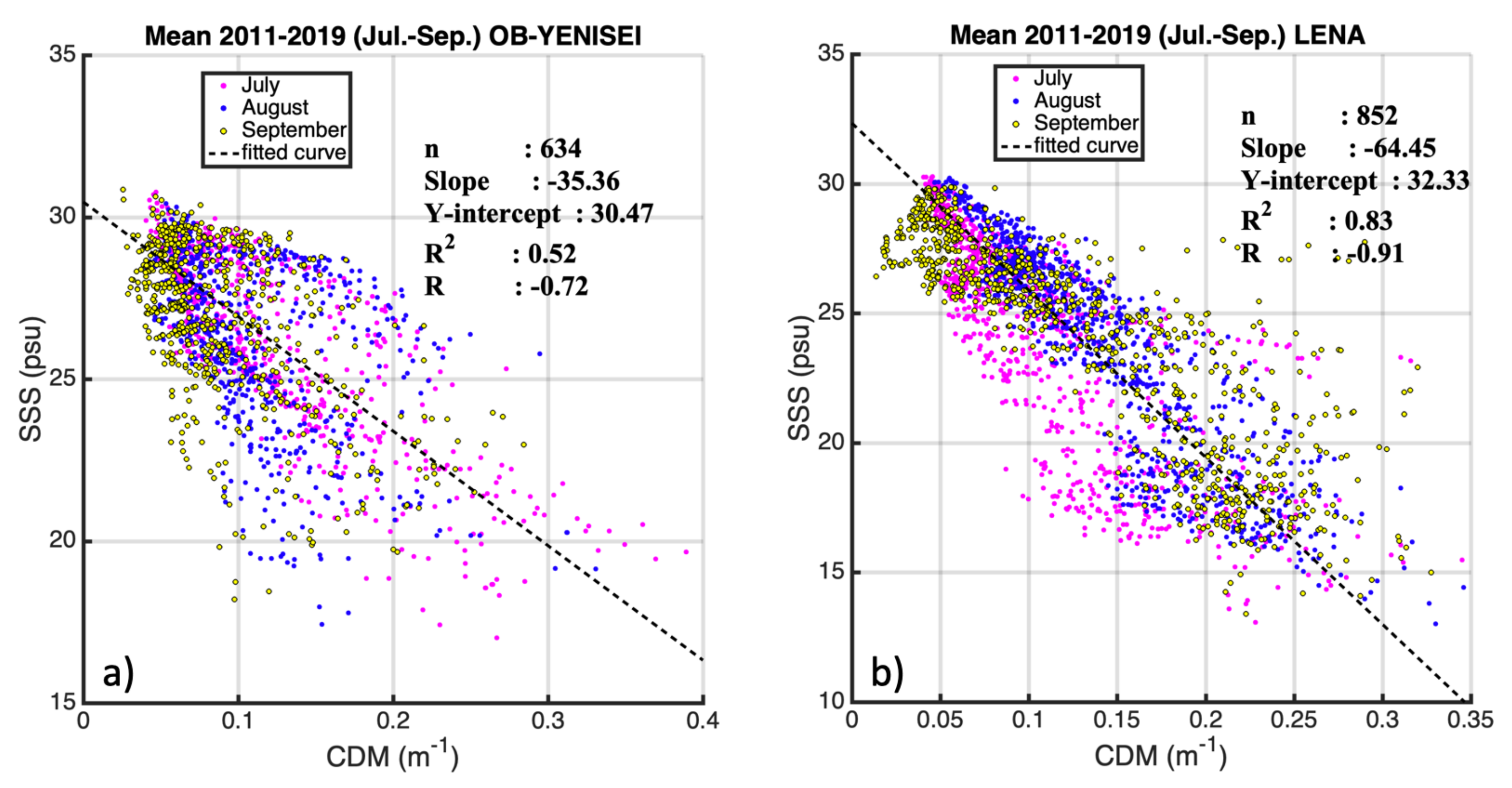
4.1. Correlation between Sea Surface Salinity and Colored Detrital Matter

We explored the capability of the newly produced SMOS SSS Arctic+ product, in conjunction with standard ocean color products, to assess the relationship between the SSS and CDM in two large Siberian rivers: the Lena and Yenisei–Ob plumes (Figure 1).
The average SSS and CDM maps throughout the ice-free summer season (July–September) from 2011 to 2019 (Figure 1) depict the spatial SSS and CDM average plume extent in the Kara and Laptev Seas, characterized by the extension of fresh and highly absorbing waters. The Kara Sea was observed to be saltier (30–34 psu) than the Laptev Sea (26–30 psu), and both Seas were affected by plume waters (fresher than ∼24–26 psu) that spread from the Ob and Yenisei Rivers to the south-eastern Kara Sea and from Lena River to the south-western Laptev Sea, up to more than 400 km northward from the river mouths [62,63]. The large river discharges are also evident in the CDM maps, as they carry higher loads of dissolved organic matter and suspended matter, associated with a higher concentration of detrital matter, with typical mean monthly values of 0.6 m 1 at the river mouth and descending to 0.05 m 1 at the edge of the plume extension delimited by 24–26 psu.
The two study areas exhibited different SSS–CDM relations. The Laptev Sea exhibited a higher, fresher FSL, but with lower CDM concentrations, compared to the Kara Sea. The CDM product for the Laptev Sea had reduced data coverage, due to cloud cover during the high discharge season, potentially reducing the average. Variations in the SSS–CDM relationships in both basins could also be attributed to geophysical characteristics (e.g., differences in vegetation, topography, and hydrology in both watersheds; differential permafrost thaw; or fires in both locations [64,65]). The delimitation of the area influenced by river plume waters—of 26 psu for the Kara Sea and 24 psu for the Laptev Sea—was chosen to illustrate the areas where the SSS and CDM co-vary as well as to be consistent with prior research characterizing these plumes [48,66].
The river plumes extension presented an interannual variation in SSS and CDM, when examining monthly means from 2011 to 2019 (see Figure A1 and Figure A2). Interannual variability in the FSL extension and mean SSS–CDM can be attributed to several processes, including variability in the hydrography coupled with wind forcing; variability in the mobilization of sediments, particles, and CDOM from catchments; different precipitation; and river discharge variability, all of which have a significant impact on the dynamics of freshwater and CDM transport to the shelf seas. Note, for example, how the plumes of the Yenisei and Ob rivers extended further north and westward in July 2017 than in 2016 (Figure A1). We can see another example of the interannual variability in the Lena plume, extending further northward in July 2015 than in July 2019. The CDM, as expected, varied with the salinity in general (the higher the CDM, the lower the SSS). However, some CDM interannual changes were not totally consistent with the SSS; for example, in the northern part of the Kara FSL, a lower CDM amount was detected in July 2018 than in July 2019 (Figure A2).
In the Kara and Laptev seas, there is an eastward freshwater transport that spreads surface-advected river plumes from the Kara to the Laptev through the Vilkitsky Strait, and from the Laptev to the East-Siberian seas through the Laptev and Sannikov straits. The effect of eastward transport [61] can be seen in satellite images (Figure A1 and Figure A2). Except for the year 2015, where fresh and highly absorbing waters extended further northward than in the rest of the study period (2011–2019), waters typically had higher CDM and lower SSS eastward of the river mouth than northward. This can be explained as follows: (i) The eastward transport is wind-driven and characterized by a quick response to synoptic variability of wind forcing [57,61]. Therefore, waters reaching east had less time to experience removal processes; (ii) it could also be related to the contributions of smaller tributaries along the coastline; or (iii) the erosion of permafrost coasts that release CDM into the coastal seas. Furthermore, waters reaching the north have generally been exposed to air-sea exchanges over longer periods and advected over larger distances from their source, therefore being more affected by removal processes such as degradation and remineralization.
Osadchiev et al. [48] have described the seasonal variability of FSL in the Kara Sea using in situ data. They found the FSL to be shallow (5–10 m deep) and fresher in the June–July discharge peak. The depth of the FSL extended (13–18 m) in August, as a result of conservative mixing with saline waters. Meanwhile, in September, the FSL is saltier and shallower (5–10 m) as a result of the mixing and decreasing river freshwater inputs [67,68]. The seasonal spreading patterns seen by satellite data are coherent with the seasonal variability described using in situ data [48]. An example for the years 2014 and 2017 with transects extracted data along the transect from the Ob river mouth (A: 73.5°E, 72°N) to the open sea (B: 73.5°E, 77.56°N) is shown in Figure 2. The FSL was fresher in July, with pronounced gradients between the FSL and seawater surroundings (Figure 2a,d,e,h), then starting to mix with saline waters in August (Figure 2b,f) and September (Figure 2c,g), leading to a freshwater area extension in the Kara Sea due to the river water effect (Figure 2d,h). Similar seasonal variability can be described following ocean color data, despite the shortage of CDM measurements in September due to cloud coverage (Figure 2k,l,o,p), with the FSL extending in August compared to July (Figure 2j,l,n,p).
The remotely sensed mean SSS and CDM from 2011 to 2019 presented strong linear negative correlations in the river-affected regions (Figure 3), with correlation coefficients of −0.72 for the Ob–Yenisei region and −0.91 for the Lena region (correlations were significant, as p-values were lower than 0.05). As expected, fresher riverine waters were associated with higher quantities of dissolved and particulate matter, and saltier marine water corresponded to lower CDM concentrations [38,57].
The correlation between SSS and CDM changed slightly over the months, from July to September (pink, blue, and yellow points in Figure 3). In the Ob–Yenisei area (Figure 3a), the slope values were −34.16 for July, −26.60 for August and −30.32 for September, while the correlation coefficients are −0.81 for July, −0.50 for August and −0.56 for September. The correlation was higher in July, due to being closer to the discharge peaks and the higher data availability due to lower cloud cover. The differences in the SSS–CDM relationships could be due to seasonal variability of the FSL, the different timing of discharge peaks in spring of Ob and Yenisei [48], the different CDM signatures of the rivers, or the different availability of data (September is more cloud covered). We discerned two different clouds of points, which could be due to different SSS–CDM signatures in the Ob and Yenisei rivers, or due to local sources of CDM causing a deviation above the linear fit.
In the Lena area (Figure 3b), the correlation between the SSS and CDM changed from July to September, with slope values ranging from −58.12 for July, −63.46 for August and −43.98 for September, while the correlation coefficients were −0.79 for July, −0.90 for August and −0.84 for September. The correlation coefficients were higher in this area over the studied period than those in the Ob–Yenisei area. The relationship between low SSS and high CDM was weaker than the relationship between high SSS and low CDM in both the Ob–Yenisei and Lena areas. In shallow coastal high CDM areas, higher CDM errors are expected due to the optical complexity of those waters and the bottom effect [69], especially in regions with an extensive shallow area as the Kara and Laptev Seas. On the other hand, the outer shelf areas, with low CDM and more stable hydrographic conditions, present the lowest errors [69]. Regarding the SSS retrievals, the Land Sea Contamination leads to biases that degrade the quality of the satellite SSS measurements at the first 50 km from the coast.
There was an interannual variation of the relationship between the SSS–CDM for the years 2011–2019 in both the Ob–Yenisei and Lena regions (Table 1), with some years exhibiting a better correlation than others. In the Lena region, the correlation coefficients ranged from −0.57 to −0.90, when years were evaluated separately. In the Ob–Yenisei region, we also found a negative linear correlations between the mean SSS as a function of mean CDM, but with lower correlation coefficients (ranging from −0.45 to −0.87); except for the year 2011, for which no clear relation was observed. The correlations were lower in this region than in the Lena region. We expect that the changes in the SSS–CDM relationship over time are primarily related to sampling limitations (i.e., as the data availability varied from year to year due to cloud coverage). The overall agreement between CDM and SSS observed by satellite in low-salinity waters was in line with the negative linear correlation observed by in situ profiles between CDOM absorption and salinity close to the river mouth by [38,40]. Using a CDOM product would have been a viable alternative option for this study, as it is a good descriptor for tracing freshwater. We chose CDM over CDOM, based on the studies of [32,70], and taking into account that river discharge contains a considerable amount of dissolved organic matter, suspended matter, and non-algal particles of terrestrial origin. The CDM product contains both particulate detritus and CDOM absorption. As their absorption coefficient spectra are similar, the particulate and dissolved terms are merged into a single product [71].
The time evolution of the mean SSS and the mean CDM in the Ob–Yenisei and Lena regions (Figure 4) showed a seasonal cycle in accordance with the River discharge cycles, as expected, based on the strong negative SSS CDM correlations. The SSS and CDM signals exhibited a strong overall anticorrelation with short-term fluctuations. In the Ob–Yenisei area (Figure 4a,b), an intense inflow of freshwater starts in late spring-early summer and relaxes in autumn [47]. Once per year, as these riverine waters reach a given area, the SSS locally drops below 28 psu, and the CDM increases. The Yenisey had a much higher discharge peak (maximum annual discharge 12 × 10 4 m 3 /s) compared to Ob (maximum annual discharge 4 × 10 4 m 3 /s) in late spring–early summer (i.e., late May–beginning of June); however, during the considered period (July–September), the discharges were similar, or the Ob even had a greater discharge (Figure 4b).
In the Lena region (Figure 4c,d), we observed a similar pattern; that is, when the river discharge increased in late spring, the surface salinity decreased up to 24 psu and the CDM started increasing. In 2013 and 2018 in the Ob–Yenisei region (Figure 4a) and 2016 in the Lena region (Figure 4c), the SSS began at such a low level that we considered those estimates to be incorrect. However, in most years, we saw an SSS transition from high (probably before break-up) to annual low (freshet), then to higher SSS in the fall (due to vertical mixing and weakening of discharge influx).
Another factor to take into account in this area is the presence of sea ice. Therefore, some salinity signatures linked to ice formation and ice retreat were expected. The time evolution of the mean sea ice concentration (SIC) from the OSISAF in the study areas (Figure 4a,b; solid light grey line) indicates how the area is deeply affected by sea ice coverage throughout the year. Overlap of mean SSS and mean SIC evolution in the study regions occurs when part of the region being averaged has ice and part of the region is ice-free. We can retrieve the SSS from July to October (ice-free months), but we need to take into account that some of the freshening observed in the SSS may originate from local sea ice melting, and not only from river discharge [67,72]. Local ice melt water should have a low CDM signature; therefore, this would allow us to distinguish between sea ice melt water and river water, as detailed in [73] where they used SSS and Ocean Color data to discriminate between water masses. However, the analysis of isotope characteristics of freshened surface layers in the Kara Sea has revealed that its volume is composed of river water directly mixed with saline water [40,74,75,76]. During late summer and autumn, the large river discharge determines the freshwater balance, while the contribution of sea ice melt is negligible [48]. Net precipitation is also expected to play a significant role in the FW distribution during open-water season in the Kara and Laptev Seas, as precipitation minus evaporation is the third major net source of FW in the Arctic Ocean and high-latitude precipitation has been increasing, as related to global warming [4,77,78].

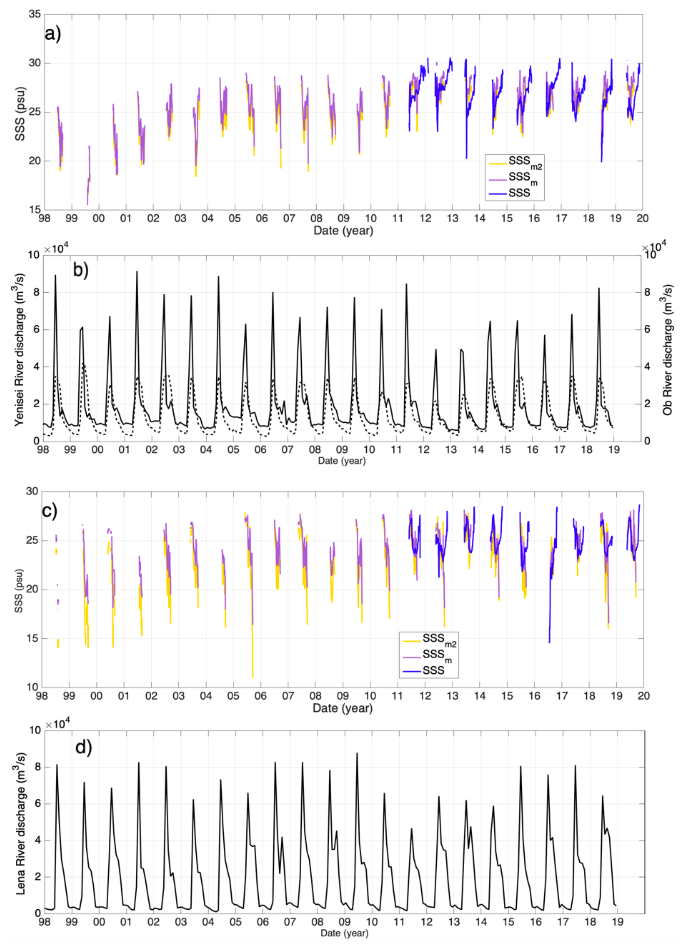
4.2. SSS Reconstruction Using Data Fusion

In this section, we construct a modeled SSS from available CDM measurements (since 1998), by exploiting the linear correlation between the two parameters and using data fusion, as described in [79,80,81,82].
Following Equation (1), we produced daily S S S f maps using CDM as a proxy. A sample map of the resulting S S S f (Figure 5c,f), the original SSS (Figure 5a,d), and proxy CDM (Figure 5b,e) are presented for 27 July 2012 (top row) and the monthly mean for July of 2012 (bottom row). Note that the original SMOS SSS lacks information close to the coast and that CDM data are affected by clouds. Furthermore, pixels with higher measurement errors close to the coastal areas are sometimes masked. S S S f had the same missing values as the CDM map, as it was used as a template to create the fused map (Equation (1)). Therefore, these type of fusion methods allow for the filling in of missing values close to the coast with physically coherent values, while maintaining the salinity structures present in the original SSS maps (Figure 5a,d).
The mean local slopes a ^ ( x ) along July, August, and September presented negative values, as the SSS decreases as the CDM increases, a behavior typically observed, as salinity is affected by major river discharges. These values were more negative close to the river mouth and increased as the plume extended. The strongest signal of river discharge corresponded to the lowest values of the local intercept b ^ ( x ) . The local intercept varied spatially, being higher far from the plume (around salinity 30), and lower in the plume-affected area and next to the mouth (around salinity 20). We assumed that these coefficients are stable in time, in order to reconstruct SSS backward in time; although this relation was expected to vary during the year, being driven by the seasonal cycle of sea ice and river flow. However, the analyzed ice-free months of July, August, and September exhibited fairly stable temporal patterns (Figure A3). The regression coefficients were impacted by the current levels of noise in SMOS at high latitudes, and are deteriorated under reduced SSS or CDM data coverage due to ice or clouds. Nevertheless, negative regression coefficients less than −0.4 are generally found in the area from 2011 to 2019, implying that the assumption of a local linear relationship between the CDM and SSS was reliable.
To construct the mean coefficients a ¯ ( x ) and b ¯ ( x ) , we averaged a ^ ( x ) and b ^ ( x ) over the months of July, August, and September for the period 2012–2019 in the river-affected area. We only used points where the local regression coefficients (Equation (9)) were lower than −0.4, to ensure the goodness of the local linear relationship and that the coefficients a ^ ( x ) and b ^ ( x ) were stable in time. The assumption of a CDM–SSS linear correlation is not valid for clear open ocean waters weakly affected by river waters; therefore, we masked all points outside the defined river-affected extended area domains: Kara Sea (60–90°E, 66–78°N) and Laptev Sea (112–144°E, 70–78°N).
Following Equation (10), we produced daily S S S m estimates from 1998 to 2020, using the CDM as a proxy and the mean coefficients a ¯ ( x ) and b ¯ ( x ) (Figure A3). Monthly means for July of the resulting S S S m for even years from 1998 to 2020 are shown in Figure A4. Inter-annual variability of the river plumes present in CDM data was translated to S S S m ; see, for example, the higher extension of the Lena plume in 2000 as compared to 2006, or higher extension of the Ob–Yenisei plume in the 2004 July monthly mean, compared to that in 2018.
An alternative modeled salinity, S S S m 2 , was obtained by using the linear regression coefficients obtained in Table 1. Linear correlation coefficients between annual mean SSS and CDM in river-affected regions were estimated by averaging the year mean slopes and y-intercepts. The mean slopes were −40.87 for Lena and −25.30 for Ob–Yenisei, and the y-intercepts was 29.19 both for Lena and Ob–Yenisei. Maps of the monthly means for July for the resulting S S S m 2 , for even years from 1998 to 2020, are shown in Figure A5. The salinity range decreased when using this alternative method, and the salinity was overestimated far from the river mouth. Over the different years, the SSS was not well-retrieved for SSS higher than 30 psu. It corresponded to the plume limit where the SSS and CDM no longer co-varied. There, at high SSS values, the CDM signal tied to salinity was weak, as it had reached the open ocean value; this result has also been observed in the Amazon plume [32]. However the S S S m estimations (Figure A4) obtained using local slope estimation a ¯ ( x ) and b ¯ ( x ) (Figure A3) performed better far from the river plume, reproducing more realistic, higher SSS.
The evolutions of the mean modeled salinity, in terms of S S S m and S S S m 2 , from 1998 to 2020 were compared with the mean SSS evolution from 2011 in the Ob–Yenisei (Figure 6a) and Lena (Figure 6c) regions, defined by black boxes in Figure 1. Means were only computed if more than 15 % CDM was present in the region. In the Lena region, S S S m 2 (Figure 6c; yellow line) tended to underestimate the salinity, as compared with S S S m (Figure 6c; purple line). Modeled salinities from ocean color followed the original temporal evolution of SMOS SSS (Figure 6; blue line) reasonably well, except at the beginning and end of each ice-free season, where cloud presence decreased the data coverage of CDM (used as a template), therefore leading to a reconstruction with low data coverage, providing an unrealistic decrease in salinity in mid-late September. Furthermore, note the unrealistic decrease in mean SSS in the Lena region (Figure 6c; blue line) in the original salinity, due to lack of data coverage for the year 2016 (Figure A1), likely due to the presence of ice.
Table 2 provides the average spatial error, by displaying the mean and the standard deviation of the difference between yearly means of modeled and original salinities from 2011 to 2019 within the two study areas. S S S m data were more precise than S S S m 2 , in terms of standard deviation and correlation coefficients. When analyzing the temporal variability of the error in both FSLs (Figure A6), the mean modeled salinity S S S m and S S S m 2 displayed similar values, when compared to the original SMOS SSS, with a common error close to 20 % at the extremes of the period, but which did not reach 10 % for the period 15 July–15 August, in comparison with SMOS. For each daily image, the reconstruction error was defined as the difference between the mean modeled SSS and the original SSS divided by the original SSS inside each region. As stated above, the errors increased at the end of each ice-free season, as the number of reconstructed pixels decreased drastically.
The SSS estimated from ocean color products, assuming conservative mixing, can be impacted by several sources of inaccuracy. Primary production and removal processes, such as CDOM degradation due to irradiance exposure or microbial degradation, are biogeochemical activities that can cause the regression line to deviate from the conservative mixing relation. CDM retrieval approaches in coastal waters, where highly absorbing waters predominate, may potentially be insufficiently precise, contributing to inaccuracies in the modeled SSS. Moreover, colored detrital matter contributes to overall attenuation in the blue region of the spectrum, where chlorophyll-a absorbs heavily, which could add errors to CDM retrievals [83,84].

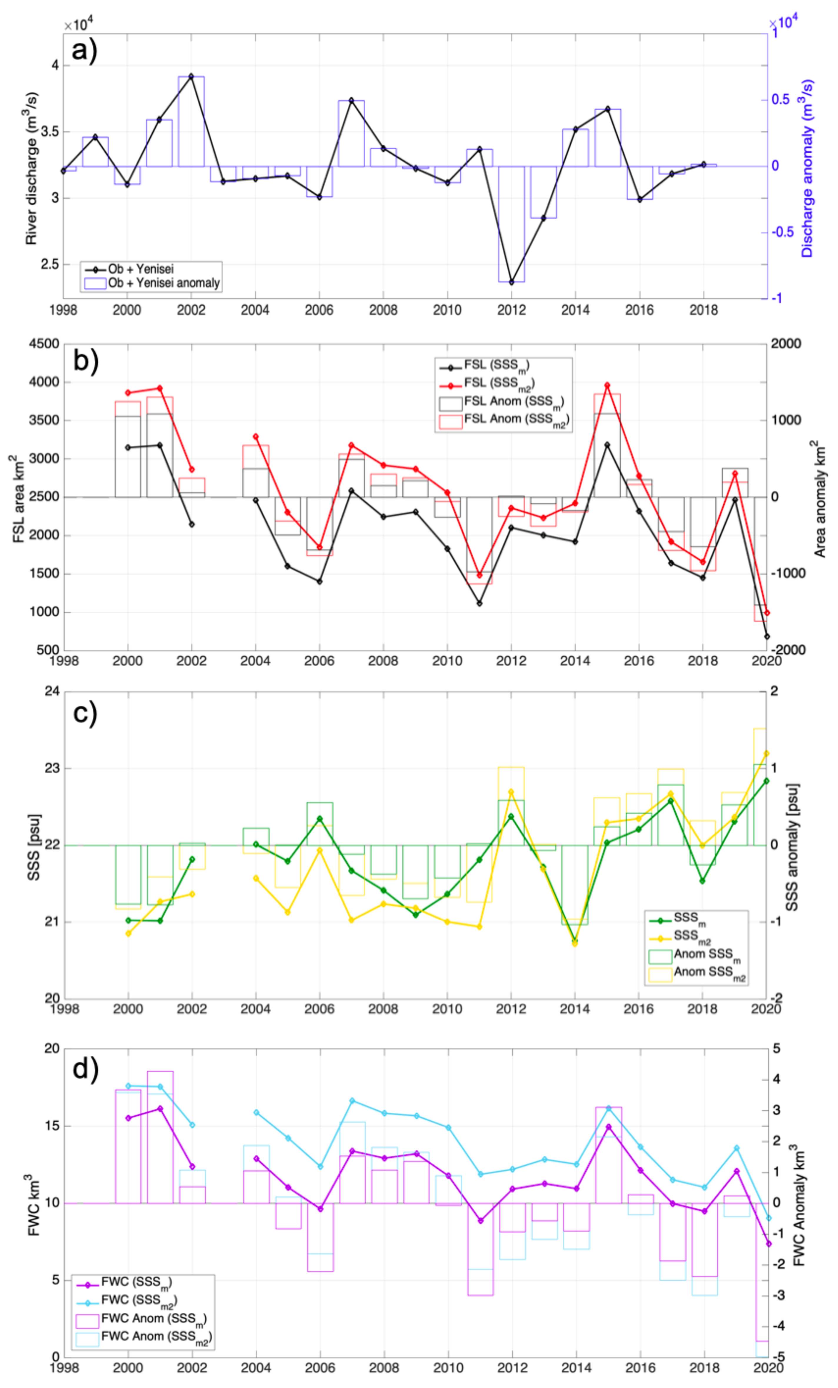
4.3. FSL Extension and Fresh Water Content

Large volumes of freshwater are discharged by the Ob and Yenisei rivers into the Kara (mean annual discharge of 427 and 673 km 3 /year from Ob and Yenisei Rivers, respectively) and Laptev (mean annual discharge of 581 km 3 /year from the Lena River) seas [39,45,85]. This freshwater volume accounts for approximately one half of the total river runoff into the Arctic Ocean. The area of the FSL extension depends on the amount of fresh water flowing into the sea, the strength and direction of summer wind forcing, and the vertical water structure of the Kara and Laptev Seas. During years with weak or predominantly westerly winds, FSL water propagates along the coast toward the East Siberian Sea; whereas, during summers with easterly or southerly winds, the plume remains on the central and northern shelf and is exportable into the Arctic Basin. The vertical structure tends to be strongly stratified during spring and summer, due to the great river discharges [68,86].
In order to estimate the annual FSL extension and the freshwater content entering the Kara and Laptev Seas, we only used the modeled S S S m and S S S m 2 reconstructions from 15 July–15 August for each year, as the accuracy of the reconstructions was higher and the data coverage was at its maximum. Years in which the data coverage for the CDM in the study region was less than 80 % were not used to estimate the extension of the FSL nor the freshwater content.
We estimated the FSL area from 1998 to 2020 by computing the area of S S S m and S S S m 2 with less than 26 psu in the Ob–Yenisei region (Figure 7, top) and less than 24 psu in the Lena region (Figure 8, top). The FSL mean area estimates in the Kara Sea were 2089 km 2 (±668 km 2 ) for S S S m and 2611 km 2 (±807 km 2 ) for S S S m 2 . Figure 7 (middle panel) shows the mean FSL area from 1998 to 2020 and the area anomaly, computed by subtracting the mean FSL area over the same period. The FSL area evolution was compared with the mean salinity evolution inside the FSL and mean river discharge volume (Figure 7, bottom panel). The salinity anomaly was computed using the mean SSS for the 1998–2020 period (Figure 7, bottom panel) and the River discharge anomalies (blue bars in Figure 7 and Figure 8, top panel) were computed by subtracting the Lena (Ob+Yenisei) river discharge mean from 1998 to 2019 [45]. Discharge anomalies of Ob+Yenisei river were correlated, as expected, with FSL area anomalies and surface salinity; that is, in general, negative discharge anomalies corresponded to negative FSL anomalies (i.e., lower extension of FSL) and with positive salinity anomalies (i.e., higher mean SSS), such as in 2012 or 2016. To the contrary, it can be observed that, in 2001, 2007, and 2015, when higher river discharge occurred, there was a larger FSL extension and lower mean SSS.
The FSL area anomaly in 2011 was clearly negative, although the river discharge anomaly was positive, which was unexpected. This could be due to the CDM extension being lower than usual after the Ob and Yenisey discharge peak (Figure 4), causing the modeled SSS to reflect the reduced FSL extension. The mean correlation coefficient for 2011 was −0.30 (Table 1), further revealing that there was no clear relationship between the original SSS and the CDM. This provides an example of how modeled salinities (and, hence, FSL extension) are dependent on the quality of the CDM estimations used as a proxy, as well as their consistency in capturing river discharge and SSS variability.
The initial volume (∼1100 km 3 ) arriving from rivers annually to the Kara Sea [85,87], mixes and dilutes with salty waters, forming freshened surface layers of ∼2089 km 2 under the S S S m methodology (and of ∼2611 km 2 under the S S S m 2 methodology), with typical FSL depth of 12 m [48]. This freshened water generates an eastward buoyancy boundary current, accounting for the large-scale zonal freshwater transport along the Siberian part of the Arctic Ocean [61].
In the Laptev Sea, the estimated FSL mean area was 2320 km 2 (±284 km 2 ) for S S S m and 2686 km 2 (±436 km 2 ) for S S S m 2 , with interannual variability as shown in Figure 8 (middle panel). Part of this extension was due to the 581 km 3 /year of freshwater annually discharged from the Lena River [85,87] mixing with the surrounding salty water, and potentially also due to the freshwater arriving from the Kara Sea spreading into the Laptev Sea, as governed by eastward Ekman transport dominant in Siberian Seas [61]. The mean FSL extension and mean salinity from 1998 to 2020 were used to compute the FSL area anomaly and SSS anomalies (Figure 8; middle and bottom panels). The Lena river discharge (Figure 8; top panel) tended to co-vary with the FSL extension positively and with the mean SSS negatively for each year. The positive discharge anomaly period from 2005 to 2009 corresponded to an increase in the FSL area and a decrease in SSS; the same was true in 2014 and 2018. The tendency to decrease river discharge in 2011 corresponded to a descline of salinity in 2011. In this area, the co-variation with Lena river discharge was not always as expected—we suspect that some of the freshwater observed was not only related to Lena river discharge, but also to other rivers discharging along the coastline (e.g., Khatanga and Olenek rivers), or transported from the Kara Sea by the eastward transport prevailing in the Siberian Seas [61].
The Freshwater Content (FWC) was estimated by integrating the freshwater fraction for the two study regions: Ob–Yenisei and Lena (Figure 7d and Figure 8d, respectively). The freshwater fraction, f, (Equation (11)) indicates the percentage of freshwater at each pixel with respect to the reference used ( S 0 = 32 for Kara Sea and S 0 = 28 for Laptev), with high values near the river mouth and low values at the FSL boundary. Figure 9 shows an example of the freshwater fraction for minimal and maximal FSL extension in the Kara Sea in 2011 (a) and 2015 (b), and the minimal and maximal FSL extension in the Laptev Sea in 2013 (c) and 2018 (d). The total liquid FWC (km 3 ) was, then, calculated by integrating f over the horizontal area and the FSL depth (Equation (12)), which we considered as a constant, based on previous references: 12 m for Kara Sea [61] and 10 m for the Laptev Sea [59,60]. In this analysis, we assumed that the FSL depth was constant to compute the FWC. The FSL thickness, on the other hand, varies with location, year, and season [60,68]. This oversimplification is a source of inaccuracy in the FWC computation, which will be assessed and addressed in future studies.
The FWC in the Kara Sea was examined from 1998 to 2020 (Figure 7d), and was found to be linked to Yenisey plus Ob river discharges, similar to the FSL extent. The minimal and maximal FSL extension in the Kara Sea in 2012 and 2015 corresponded to the minimal and maximal FWC extent. The mean FWC in the Ob–Yenisei region (Kara sea) estimated from S S S m was 11.85 km 3 (±2.22 km 3 ), while the mean FWC estimated from S S S m 2 was 14.02 km 3 (±2.32 km 3 ). Thus, the approximately mean 1100 km 3 /year of freshwater entering annually from the Ob–Yenisei rivers [87] would extend in freshened surface layers of 2089 km 2 (or 2611 km 2 for S S S m ) into the Kara Sea, with a typical depths of 12 m [61], which would contain approximately 11.85–14.02 km 3 of freshwater, when S 0 = 32 .
The FWC evolution in the Laptev Sea (Figure 8d) indicated that, as in the case of FSL extent, it was correlated with the Lena river discharge. Years corresponding to freshwater maxima coincided with those having a maximum FSL extent (i.e., 2008 and 2018). Analogously, years having the smallest FSL extent (i.e., 2005 and 2013) corresponded to those with freshwater minima, implying that the FSL extension is mainly due to the amount of river water entering the Laptev Sea. For the period 1998–2020, the mean FWC in the Lena region (Laptev Sea) was 10.15 km 3 (±0.93 km 3 ) when estimated using S S S m ; meanwhile, it was 12.45 km 3 (±1.48 km 3 ), when estimated using S S S m 2 . The estimates of FWC and FSL extension from S S S m had lower standard deviations than when estimated from S S S m 2 . For the Lena river, the mean 581 km 3 /year discharging annually into the Laptev Sea [87] would form a freshened surface layer of 2320 km 2 (or 2686 km 2 for S S S m 2 ), with typical depth of 10 m [59,60] and FWC of 10.15–12.44 km 3 of freshwater, when S 0 = 28 .

5. Conclusions

We used the recently released SMOS SSS Arctic+ product in combination with a satellite CDM ocean color product in order to study the dynamics and interannual variations of freshened surface layers (FSLs) created by the discharges of the main Siberian rivers—the Lena, Ob, and Yenisei—into the Laptev and Kara Seas. The combination of fresh river water and saltier sea water on the Siberian shelf of the Laptev and Kara Seas produced extensive FSLs, with a typical thickness of 10–20 m in depth. Ocean water properties were considered to follow a conservative mixing assumption when affected by dilution processes. CDM maps associate FSL (areas with SSS lower than 26 psu in the Kara Sea and less than 24 psu in the Laptev Sea) with greater concentrations of detrital matter than in the surrounding marine water, with mean monthly values of ∼0.6 m 1 near the river mouth and ∼0.05 m 1 at the edge of the FSL. Satellite images show that waters tend to have higher CDM east of the river mouth than northward, probably due to the eastward transportation of freshwater in the Kara and Laptev seas. As a result, this extends the surface-advected FSL from the Kara to the Laptev Sea and from the Laptev to the East-Siberian seas. Waters advected northward from the river mouth to the Siberian seas have high salinity and low CDM [84].
The satellite data also revealed seasonal spreading dynamics. The FSL was fresher in July, with noticeable gradients between the FSL and the surrounding seawater. Then, the FSL area extended as it mixed with saline water in August. The inflow of the river water was reduced in September, resulting in a smaller affected area. Cloud cover had an adverse effect on CDM images. The number of missing points increased in September, although estimates for July and August showed reasonable coverage for the majority of the considered period. The impact of freshwater inflow from sea ice melting is likely to be minor, as the entire region was nearly ice-free from July. During the period 2011–2019 (i.e., the period of SMOS salinity maps availability), the FSL extension presented interannual variability. The amount of CDM along the FSL also varied from year to year. With mean correlation coefficients of −0.74 for the Kara Sea and −0.92 for the Laptev Sea, we observed a high negative correlation between the mean SSS and CDM, with short-term oscillations inside the FSL of the Kara and Laptev Seas, demonstrating that CDM co-varies with salinity, as expected (i.e., higher CDM values where the SSS is fresher), which is consistent with prior research describing similar plumes during the ice-free summer season [38,62].
Assuming conservative mixing in the FSL of the Kara and Laptev Seas, the SSS was estimated from ocean color, going all the way back to 1998. The negative linear relationship between the SSS and CDM was used to model one variable, using the other as a proxy, from 1998 to 2020 using two distinct methodologies. The key difference between these methods was that the coefficients used to generate S S S m varied spatially across the region, whereas those used to generate S S S m 2 were the same scalars in each region. When utilizing the latter approach (i.e., S S S m 2 ), the salinity range was reduced, and the salinity was overestimated far from the river mouth. The S S S m 2 is not well-recovered for SSS higher than 30 psu in different years at the FSL limit, where the SSS and CDM no longer co-varied. However, outside the FSL area, the S S S m predictions performed better, recreating realistically higher SSS. Overall, the methods for modeling SSS based on the conservative mixing relationship corresponded well to the original SMOS SSS data from 2011 to 2019 in the FSL. Except at the start and end of each ice-free season, when CDM data coverage dropped due to the presence of clouds, salinities modeled from ocean color accurately reflected the original temporal evolution of the SMOS SSS, with a typical error of less than 20 % .
The largest sources of potential errors expected when retrieving the SSS from CDM using the conservative mixing assumption are: (a) Potential inaccuracies of satellite products and errors in retrieving algorithms, especially close to the coast and sea-ice, and (b) in places where the CDM is not only acting as a passive tracer of freshwater but is affected by biogeochemical processes such as primary production or degradation. The method could be extended to other regions of the Arctic affected by large rivers, such as the Kolyma, Yukon, and Mackenzie, in order to monitor trends in Freshwater content.
The inferred SSS during the ice-free periods of 1998 to 2020 was used to estimate the extension and freshwater content of the FSL in the Kara and Laptev Seas. To do so, we used the mean modeled S S S m and S S S m 2 from 15 July to 15 August, as the reconstruction accuracy was higher and the data coverage was optimal in this period. The annual river flow into the Kara Sea mixes and dilutes with salty waters, resulting in a FSL extension of 2089 km 2 with S S S m (and 2611 km 2 with S S S m 2 ). Discharge anomalies, as expected, were correlated with FSL area anomalies and surface salinity, with negative discharge anomalies corresponding to lower FSL extension and positive discharge anomalies corresponding to higher mean SSS. The estimated FSL mean area in the Laptev Sea was 2320 km 2 for S S S m (and 2686 km 2 for S S S m ). The Freshwater Content (FWC) was calculated by integrating the freshwater fraction over the horizontal area and the depth of the FSL in the Kara Sea and the Laptev Sea for the period 1998–2020. When S 0 = 32 was chosen as the reference salinity, the freshened surface layers in the Kara Sea would contain approximately 11.85–14.02 km 3 of freshwater (roughly half of the total extension of FSL). Furthermore, when S 0 = 28 is used, the freshwater content in the Laptev Sea would be 10.15–12.44 km 3 (less than half of the total extent of FSL). The years when the FSL reached its maximum/minimum extent corresponded to freshwater content maxima/minima, respectively, demonstrating that the FSL extension is primarily determined by the amount of river water entering the Kara and Laptev Seas.
These promising results suggest that the SMOS SSS has the potential to better monitor river discharge changes in the Eurasian Basin and to assess the Arctic freshwater system throughout the ice-free season and encourage the exploration of further ocean color–surface salinity comparisons. SMOS SSS has the potential to aid in determining the region’s circulation, which is impacted by variances in the buoyancy of river-affected fresher and saltier ocean water as well as changes in the prevailing wind. The reported increase in river runoff since the 1940s [1] is primarily produced during the winter–spring period, whereas discharge during the flooding period (late spring–summer) has remained nearly constant [45]. Our FSL extent estimation was based on the July-September period from 1998 to 2020. It is not within the scope of this study to discern a climatic trend. Long-term trends and their implications can be addressed in future studies. However, the future acquisition of remotely sensed surface salinity data with the CMIR ESA mission should allow us to examine climatic patterns using at least 30 years of data. Continuous efforts in acquiring and exploiting remotely sensed SSS and optical data will allow us to understand the complex relationships and feedbacks between sea ice formation, river discharges, and stratification in the Arctic Ocean.

Author Contributions

Conceptualization, M.U. and C.G.; methodology, M.U., C.G. and E.O.; software, M.U.; validation, M.U., R.G.-A. and S.G.; formal analysis, M.U.; investigation, M.U., C.G. and R.G.-A.; data curation, M.U., J.M. and S.G.; writing original draft preparation, M.U.; writing, review and editing, C.G., R.G.-A., J.M. and E.O.; supervision, C.G. and E.O.; project administration, M.U. and C.G.; funding acquisition, M.U. All authors have read and agreed to the published version of the manuscript.

Funding

M. Umbert was funded by the European Union’s Horizon 2020 research and innovation program under the Marie Skłodowska-Curie Individual Fellowship Career Restart Panel (MSCA-IF-EF-CAR Number 840374). R. Gonçalves-Araujo has received funding from the European Union’s Horizon 2020 research and innovation program under the Marie Skłodowska-Curie Grant Agreement No. 839311. This research was funded by the Spanish government, through the ‘Severo Ochoa Centre of Excellence’ accreditation (CEX2019-000928-S).

Institutional Review Board Statement

Not applicable.

Informed Consent Statement

Not applicable.

Data Availability Statement

Data sharing not applicable.

Acknowledgments

This work represents a contribution to the CSIC Thematic Interdisciplinary Platform PTI POLARCSIC and PTI TELEDETECT. The authors acknowledge the collaboration of Alexander Shiklomanov from the University of New Hampshire, for providing filtered river discharge data. This manuscript is part of a project that has received funding from the European Union’s Horizon 2020 research and innovation programme under the Marie Skłodowska-Curie Grant Agreement No. 840374 and No. 839311. We acknowledge the insightful reviews, comments, and suggestions from two anonymous reviewers, which helped to improve the content and readability of the manuscript.

Conflicts of Interest

The authors declare no conflict of interest.

Appendix A. Additional Figures

Figure A1. The July monthly mean of the SMOS SSS maps for 2011–2019. The mean monthly isohaline of 26 psu is shown as a solid black line, and the isohaline of 24 psu is shown as a solid red line.
Remotesensing 13 03828 g0a1
Figure A2. The July monthly means of CDM for 2011–2019. The mean monthly isohaline of 26 psu is shown as a solid black line, and the isohaline of 24 psu is shown as a solid red line.
Remotesensing 13 03828 g0a2
Figure A3. Temporal means of the local slope estimation a ¯ ( x ) (top left) and local intercept estimation b ¯ ( x ) (top right). Temporal standard deviation of the local slope estimation a ¯ ( x ) (bottom left) and local intercept estimation b ¯ ( x ) (bottom right).
Remotesensing 13 03828 g0a3
Figure A4. Monthly mean of S S S m for July for even years from 1998 to 2020, from the original CDM, using a ¯ ( x ) and b ¯ ( x ) coefficients (only even years are shown). The mean monthly isohaline of 26 psu (24 psu) shown as solid black (red) line.
Remotesensing 13 03828 g0a4
Figure A5. Monthly mean S S S m 2 for July for even years from 1998 to 2020, from the original CDM, using a ¯ ( x ) and b ¯ ( x ) coefficients (only even years are shown).
Remotesensing 13 03828 g0a5
Figure A6. Error estimation for S S S m (purple discontinuous line) and S S S m 2 (yellow discontinuous line) in Yenisei–Ob (top) and Lena regions (bottom). The error is defined as the difference between the mean modeled SSS and the original SSS, divided by the original SSS.
Remotesensing 13 03828 g0a6

References

  1. Poloczanska, E.; Mintenbeck, K.; Portner, H.O.; Roberts, D.; Levin, L.A. The IPCC special report on the ocean and cryosphere in a changing climate. In Proceedings of the 2018 Ocean Sciences Meeting, Portland, OR, USA, 11–16 February 2018. [Google Scholar]
  2. Thoman, R.L.; Bhatt, U.S.; Bieniek, P.A.; Brettschneider, B.R.; Brubaker, M.; Danielson, S.; Labe, Z.; Lader, R.; Meier, W.N.; Sheffield, G.; et al. The Record Low Bering Sea Ice Extent in 2018: Context, Impacts, and an Assessment of the Role of Anthropogenic Climate Change. 2020. Available online: https://journals.ametsoc.org/view/journals/bams/101/1/bams-d-19-0175.1.xml?tab_body=previewPdf-43621 (accessed on 31 July 2021).
  3. National Snow and Ice Data Center. Available online: https://nsidc.org/arcticseaicenews/2020/ (accessed on 31 July 2021).
  4. Haine, T.W.; Curry, B.; Gerdes, R.; Hansen, E.; Karcher, M.; Lee, C.; Rudels, B.; Spreen, G.; de Steur, L.; Stewart, K.D.; et al. Arctic freshwater export: Status, mechanisms, and prospects. Glob. Planet. Chang. 2015, 125, 13–35. [Google Scholar] [CrossRef] [Green Version]
  5. Proshutinsky, A.; Krishfield, R.; Toole, J.; Timmermans, M.L.; Williams, W.; Zimmermann, S.; Yamamoto-Kawai, M.; Armitage, T.; Dukhovskoy, D.; Golubeva, E.; et al. Analysis of the Beaufort Gyre freshwater content in 2003–2018. J. Geophys. Res. Ocean. 2019, 124, 9658–9689. [Google Scholar] [CrossRef] [PubMed] [Green Version]
  6. Solomon, A.; Heuzé, C.; Rabe, B.; Bacon, S.; Bertino, L.; Heimbach, P.; Inoue, J.; Iovino, D.; Mottram, R.; Zhang, X.; et al. Freshwater in the Arctic Ocean 2010–2019. Ocean Sci. 2021, 17, 1081–1102. [Google Scholar] [CrossRef]
  7. Haas, C.; Pfaffling, A.; Hendricks, S.; Rabenstein, L.; Etienne, J.L.; Rigor, I. Reduced ice thickness in Arctic Transpolar Drift favors rapid ice retreat. Geophys. Res. Lett. 2008, 35. [Google Scholar] [CrossRef] [Green Version]
  8. Carmack, E.; Polyakov, I.; Padman, L.; Fer, I.; Hunke, E.; Hutchings, J.; Jackson, J.; Kelley, D.; Kwok, R.; Layton, C.; et al. Toward quantifying the increasing role of oceanic heat in sea ice loss in the new Arctic. Bull. Am. Meteorol. Soc. 2015, 96, 2079–2105. [Google Scholar] [CrossRef]
  9. Wang, Q.; Wekerle, C.; Danilov, S.; Sidorenko, D.; Koldunov, N.; Sein, D.; Rabe, B.; Jung, T. Recent sea ice decline did not significantly increase the total liquid freshwater content of the Arctic Ocean. J. Clim. 2019, 32, 15–32. [Google Scholar] [CrossRef] [Green Version]
  10. Timmermans, M.L.; Marshall, J. Understanding Arctic Ocean circulation: A review of ocean dynamics in a changing climate. J. Geophys. Res. Ocean. 2020, 125. [Google Scholar] [CrossRef]
  11. Savelieva, N.; Semiletov, I.; Vasilevskaya, L.; Pugach, S. A climate shift in seasonal values of meteorological and hydrological parameters for Northeastern Asia. Prog. Oceanogr. 2000, 47, 279–297. [Google Scholar] [CrossRef]
  12. Lammers, R.B.; Shiklomanov, A.I.; Vörösmarty, C.J.; Fekete, B.M.; Peterson, B.J. Assessment of contemporary Arctic river runoff based on observational discharge records. J. Geophys. Res. Atmos. 2001, 106, 3321–3334. [Google Scholar] [CrossRef]
  13. Peterson, B.J.; Holmes, R.M.; McClelland, J.W.; Vörösmarty, C.J.; Lammers, R.B.; Shiklomanov, A.I.; Shiklomanov, I.A.; Rahmstorf, S. Increasing river discharge to the Arctic Ocean. Science 2002, 298, 2171–2173. [Google Scholar] [CrossRef] [Green Version]
  14. Peterson, B.J.; McClelland, J.; Curry, R.; Holmes, R.M.; Walsh, J.E.; Aagaard, K. Trajectory shifts in the Arctic and subarctic freshwater cycle. Science 2006, 313, 1061–1066. [Google Scholar] [CrossRef]
  15. Rennermalm, A.K.; Wood, E.F.; Déry, S.J.; Weaver, A.J.; Eby, M. Sensitivity of the thermohaline circulation to Arctic Ocean runoff. Geophys. Res. Lett. 2006, 33. [Google Scholar] [CrossRef]
  16. Soppa, M.A.; Pefanis, V.; Hellmann, S.; Losa, S.N.; Hölemann, J.; Martynov, F.; Heim, B.; Janout, M.A.; Dinter, T.; Rozanov, V.; et al. Assessing the influence of water constituents on the radiative heating of Laptev Sea shelf waters. Front. Mar. Sci. 2019, 6, 221. [Google Scholar] [CrossRef]
  17. Fournier, S.; Lee, T.; Wang, X.; Armitage, T.W.; Wang, O.; Fukumori, I.; Kwok, R. Sea surface salinity as a proxy for Arctic Ocean freshwater changes. J. Geophys. Res. Ocean. 2020, 125, e2020JC016110. [Google Scholar] [CrossRef]
  18. Supply, A.; Boutin, J.; Vergely, J.L.; Kolodziejczyk, N.; Reverdin, G.; Reul, N.; Tarasenko, A. New insights into SMOS sea surface salinity retrievals in the Arctic Ocean. Remote Sens. Environ. 2020, 249, 112027. [Google Scholar] [CrossRef]
  19. Kerr, Y.; Waldteufel, P.; Wigneron, J.; Delwart, S.; Cabot, F.; Boutin, J.; Escorihuela, M.; Font, J.; Reul, N.; Gruhier, C.; et al. The SMOS Mission: New Tool for Monitoring Key Elements of the Global Water Cycle. Proc. IEEE 2010, 98, 666–687. [Google Scholar] [CrossRef] [Green Version]
  20. Mecklenburg, S.; Drusch, M.; Kerr, Y.H.; Font, J.; Martin-Neira, M.; Delwart, S.; Buenadicha, G.; Reul, N.; Daganzo-Eusebio, E.; Oliva, R.; et al. ESA’s soil moisture and ocean salinity mission: Mission performance and operations. IEEE Trans. Geosci. Remote Sens. 2012, 50, 1354–1366. [Google Scholar] [CrossRef] [Green Version]
  21. Reul, N.; Grodsky, S.; Arias, M.; Boutin, J.; Catany, R.; Chapron, B.; d’Amico, F.; Dinnat, E.; Donlon, C.; Fore, A.; et al. Sea surface salinity estimates from spaceborne L-band radiometers: An overview of the first decade of observation (2010–2019). Remote Sens. Environ. 2020, 242, 111769. [Google Scholar] [CrossRef]
  22. Olmedo, E.; Gabarró, C.; González-Gambau, V.; Martínez, J.; Ballabrera-Poy, J.; Turiel, A.; Portabella, M.; Fournier, S.; Lee, T. Seven years of SMOS sea surface salinity at high latitudes: Variability in Arctic and Sub-Arctic regions. Remote Sens. 2018, 10, 1772. [Google Scholar] [CrossRef] [Green Version]
  23. Martínez, J. Arctic+ Salinity: Algorithm Theoretical Baseline Document; Technical Report; Argans LTD: Plymouth, UK, 2020. [Google Scholar] [CrossRef]
  24. Martínez, J.; Gabarró, C.; Turiel, A. Arctic Sea Surface Salinity L2 orbits and L3 maps (V.3.1) [Dataset]. Technical Report. 2020. Available online: https://digital.csic.es/handle/10261/219679 (accessed on 31 July 2021). [CrossRef]
  25. Organelli, E.; Bricaud, A.; Gentili, B.; Antoine, D.; Vellucci, V. Retrieval of Colored Detrital Matter (CDM) light absorption coefficients in the Mediterranean Sea using field and satellite ocean color radiometry: Evaluation of bio-optical inversion models. Remote Sens. Environ. 2016, 186, 297–310. [Google Scholar] [CrossRef]
  26. Bowers, D.; Brett, H. The relationship between CDOM and salinity in estuaries: An analytical and graphical solution. J. Mar. Syst. 2008, 73, 1–7. [Google Scholar] [CrossRef]
  27. Nakada, S.; Kobayashi, S.; Hayashi, M.; Ishizaka, J.; Akiyama, S.; Fuchi, M.; Nakajima, M. High-resolution surface salinity maps in coastal oceans based on geostationary ocean color images: Quantitative analysis of river plume dynamics. J. Oceanogr. 2018, 74, 287–304. [Google Scholar] [CrossRef]
  28. Ferrari, G.; Dowell, M. CDOM absorption characteristics with relation to fluorescence and salinity in coastal areas of the southern Baltic Sea. Estuar. Coast. Shelf Sci. 1998, 47, 91–105. [Google Scholar] [CrossRef]
  29. Binding, C.; Bowers, D. Measuring the salinity of the Clyde Sea from remotely sensed ocean colour. Estuar. Coast. Shelf Sci. 2003, 57, 605–611. [Google Scholar] [CrossRef]
  30. Urquhart, E.A.; Zaitchik, B.F.; Hoffman, M.J.; Guikema, S.D.; Geiger, E.F. Remotely sensed estimates of surface salinity in the Chesapeake Bay: A statistical approach. Remote Sens. Environ. 2012, 123, 522–531. [Google Scholar] [CrossRef]
  31. Korosov, A.; Counillon, F.; Johannessen, J.A. Monitoring the spreading of the A mazon freshwater plume by MODIS, SMOS, A quarius, and TOPAZ. J. Geophys. Res. Ocean. 2015, 120, 268–283. [Google Scholar] [CrossRef]
  32. Fournier, S.; Chapron, B.; Salisbury, J.; Vandemark, D.; Reul, N. Comparison of spaceborne measurements of sea surface salinity and colored detrital matter in the Amazon plume. J. Geophys. Res. Ocean. 2015, 120, 3177–3192. [Google Scholar] [CrossRef] [Green Version]
  33. Hu, C.; Muller-Karger, F.E.; Biggs, D.C.; Carder, K.L.; Nababan, B.; Nadeau, D.; Vanderbloemen, J. Comparison of ship and satellite bio-optical measurements on the continental margin of the NE Gulf of Mexico. Int. J. Remote Sens. 2003, 24, 2597–2612. [Google Scholar] [CrossRef]
  34. Chen, S.; Hu, C. Estimating sea surface salinity in the northern Gulf of Mexico from satellite ocean color measurements. Remote Sens. Environ. 2017, 201, 115–132. [Google Scholar] [CrossRef]
  35. Del Castillo, C.E.; Miller, R.L. On the use of ocean color remote sensing to measure the transport of dissolved organic carbon by the Mississippi River Plume. Remote Sens. Environ. 2008, 112, 836–844. [Google Scholar] [CrossRef] [Green Version]
  36. Bai, Y.; Pan, D.; Cai, W.J.; He, X.; Wang, D.; Tao, B.; Zhu, Q. Remote sensing of salinity from satellite-derived CDOM in the Changjiang River dominated East China Sea. J. Geophys. Res. Ocean. 2013, 118, 227–243. [Google Scholar] [CrossRef]
  37. Granskog, M.A.; Macdonald, R.W.; Mundy, C.J.; Barber, D.G. Distribution, characteristics and potential impacts of chromophoric dissolved organic matter (CDOM) in Hudson Strait and Hudson Bay, Canada. Cont. Shelf Res. 2007, 27, 2032–2050. [Google Scholar] [CrossRef]
  38. Gonçalves-Araujo, R.; Stedmon, C.A.; Heim, B.; Dubinenkov, I.; Kraberg, A.; Moiseev, D.; Bracher, A. From fresh to marine waters: Characterization and fate of dissolved organic matter in the Lena River Delta Region, Siberia. Front. Mar. Sci. 2015, 2, 108. [Google Scholar] [CrossRef] [Green Version]
  39. Alling, V.; Sanchez-Garcia, L.; Porcelli, D.; Pugach, S.; Vonk, J.E.; Van Dongen, B.; Mörth, C.M.; Anderson, L.G.; Sokolov, A.; Andersson, P.; et al. Nonconservative behavior of dissolved organic carbon across the Laptev and East Siberian seas. Glob. Biogeochem. Cycles 2010, 24. [Google Scholar] [CrossRef]
  40. Hölemann, J.A.; Juhls, B.; Bauch, D.; Janout, M.; Koch, B.P.; Heim, B. The impact of the freeze–melt cycle of land-fast ice on the distribution of dissolved organic matter in the Laptev and East Siberian seas (Siberian Arctic). Biogeosciences 2021, 18, 3637–3655. [Google Scholar] [CrossRef]
  41. Drozdova, A.N.; Nedospasov, A.A.; Lobus, N.V.; Patsaeva, S.V.; Shchuka, S.A. CDOM Optical Properties and DOC Content in the Largest Mixing Zones of the Siberian Shelf Seas. Remote Sens. 2021, 13, 1145. [Google Scholar] [CrossRef]
  42. Juhls, B.; Overduin, P.P.; Hölemann, J.; Hieronymi, M.; Matsuoka, A.; Heim, B.; Fischer, J. Dissolved organic matter at the fluvial–marine transition in the Laptev Sea using in situ data and ocean colour remote sensing. Biogeosciences 2019, 16, 2693–2713. [Google Scholar] [CrossRef] [Green Version]
  43. Glukhovets, D.I.; Goldin, Y.A. Surface desalinated layer distribution in the Kara Sea determined by shipboard and satellite data. Oceanologia 2020, 62, 364–373. [Google Scholar] [CrossRef]
  44. Holmes, R.M.; McClelland, J.W.; Peterson, B.J.; Tank, S.E.; Bulygina, E.; Eglinton, T.I.; Gordeev, V.V.; Gurtovaya, T.Y.; Raymond, P.A.; Repeta, D.J.; et al. Seasonal and annual fluxes of nutrients and organic matter from large rivers to the Arctic Ocean and surrounding seas. Estuaries Coasts 2012, 35, 369–382. [Google Scholar] [CrossRef]
  45. Shiklomanov, A.; Déry, S.; Tretiakov, M.; Yang, D.; Magritsky, D.; Georgiadi, A.; Tang, W. River Freshwater Flux to the Arctic Ocean. In Arctic Hydrology, Permafrost and Ecosystems; Yang, D., Kane, D.L., Eds.; Springer International Publishing: Cham, Switzerland, 2021; pp. 703–738. [Google Scholar] [CrossRef]
  46. Aagaard, K.; Carmack, E.C. The role of sea ice and other fresh water in the Arctic circulation. J. Geophys. Res. Ocean. 1989, 94, 14485–14498. [Google Scholar] [CrossRef]
  47. Harms, I.; Karcher, M. Kara Sea freshwater dispersion and export in the late 1990s. J. Geophys. Res. Ocean. 2005, 110. [Google Scholar] [CrossRef] [Green Version]
  48. Osadchiev, A.; Frey, D.; Shchuka, S.; Tilinina, N.; Morozov, E.; Zavialov, P. Structure of the freshened surface layer in the Kara Sea during ice-free periods. J. Geophys. Res. Ocean. 2021, 126, e2020JC016486. [Google Scholar] [CrossRef]
  49. Demidov, A.; Gagarin, V.; Vorobieva, O.; Makkaveev, P.; Artemiev, V.; Khrapko, A.; Grigoriev, A.; Sheberstov, S. Spatial and vertical variability of primary production in the Kara Sea in July and August 2016: The influence of the river plume and subsurface chlorophyll maxima. Polar Biol. 2018, 41, 563–578. [Google Scholar] [CrossRef]
  50. Lavergne, T.; Sørensen, A.M.; Kern, S.; Tonboe, R.; Notz, D.; Aaboe, S.; Bell, L.; Dybkjær, G.; Eastwood, S.; Gabarro, C.; et al. Version 2 of the EUMETSAT OSI SAF and ESA CCI sea-ice concentration climate data records. Cryosphere 2019, 13, 49–78. [Google Scholar] [CrossRef] [Green Version]
  51. EUMETSAT Ocean and Sea Ice Satellite Application Facility. Global Sea Ice Concentration Climate Data Record 1979–2015 (v2.0, 2017); Norwegian and Danish Meteorological Institutes: Darmstadt, Germany, 2017. [Google Scholar] [CrossRef]
  52. EUMETSAT Ocean and Sea Ice Satellite Application Facility. Global Sea Ice Concentration Interim Climate Data Record 2016 Onwards (v2.0, 2019); Norwegian and Danish Meteorological Institutes: Darmstadt, Germany, 2019. [Google Scholar]
  53. Shiklomanov, A.I.; Holmes, R.M.; McClelland, J.W.; Tank, S.E.; Spencer, R.G.M. Arctic Great Rivers Observatory. Discharge Dataset, Version 20180527. Technical Report. 2021. [Google Scholar]
  54. Nieves, V.; Llebot, C.; Turiel, A.; Solé, J.; García-Ladona, E.; Estrada, M.; Blasco, D. Common turbulent signature in sea surface temperature and chlorophyll maps. Geophys. Res. Lett. 2007, 34, L23602. [Google Scholar] [CrossRef] [Green Version]
  55. Polyakova, Y.I.; Kryukova, I.; Martynov, F.; Novikhin, A.; Abramova, E.; Kassens, H.; Hölemann, J. Community structure and spatial distribution of phytoplankton in relation to hydrography in the Laptev Sea and the East Siberian Sea (autumn 2008). Polar Biol. 2021, 1–22. [Google Scholar] [CrossRef]
  56. Zatsepin, A.; Kremenetskiy, V.; Kubryakov, A.; Stanichny, S.; Soloviev, D. Propagation and transformation of waters of the surface desalinated layer in the Kara Sea. Oceanology 2015, 55, 450–460. [Google Scholar] [CrossRef]
  57. Kubryakov, A.; Stanichny, S.; Zatsepin, A. River plume dynamics in the Kara Sea from altimetry-based lagrangian model, satellite salinity and chlorophyll data. Remote Sens. Environ. 2016, 176, 177–187. [Google Scholar] [CrossRef]
  58. Paclov, V.; Timokhov, L.; Baskakov, G.; Kulakov, M.Y.; Kurazhov, V. Hydrometeorological Regime of the Kara, Laptev, and East-Siberian Seas; Technical Report; Washington Univ Seattle Applied Physics Lab: Seattle, WA, USA, 1996. [Google Scholar]
  59. Conrad, S.; Ingri, J.; Gelting, J.; Nordblad, F.; Engström, E.; Rodushkin, I.; Andersson, P.S.; Porcelli, D.; Gustafsson, Ö.; Semiletov, I.; et al. Distribution of Fe isotopes in particles and colloids in the salinity gradient along the Lena River plume, Laptev Sea. Biogeosciences 2019, 16, 1305–1319. [Google Scholar] [CrossRef] [Green Version]
  60. Janout, M.; Hölemann, J.; Laukert, G.; Smirnov, A.; Krumpen, T.; Bauch, D.; Timokhov, L. On the variability of stratification in the freshwater-influenced Laptev Sea region. Front. Mar. Sci. 2020. [Google Scholar] [CrossRef]
  61. Osadchiev, A.; Pisareva, M.; Spivak, E.; Shchuka, S.; Semiletov, I. Freshwater transport between the Kara, Laptev, and East-Siberian seas. Sci. Rep. 2020, 10, 113041. [Google Scholar]
  62. Heim, B.; Juhls, B.; Abramova, E.; Bracher, A.; Doerffer, R.; Gonçalves-Araujo, R.; Hellman, S.; Kraberg, A.; Martynov, F.; Overduin, P. Ocean colour remote sensing in the Laptev Sea. In Remote Sensing of the Asian Seas; Springer: Berlin/Heidelberg, Germany, 2019; pp. 123–138. [Google Scholar]
  63. Gonçalves-Araujo, R.; Juhls, B. Dissolved Organic Matter in the Lena River Delta Region, Siberia, Russia. 2019. Available online: https://repository.geologyscience.ru/handle/123456789/8007 (accessed on 31 July 2021). [CrossRef]
  64. McClelland, J.W.; Holmes, R.M.; Peterson, B.J.; Stieglitz, M. Increasing river discharge in the Eurasian Arctic: Consideration of dams, permafrost thaw, and fires as potential agents of change. J. Geophys. Res. Atmos. 2004, 109. [Google Scholar] [CrossRef] [Green Version]
  65. Walker, S.A.; Amon, R.M.; Stedmon, C.A. Variations in high-latitude riverine fluorescent dissolved organic matter: A comparison of large Arctic rivers. J. Geophys. Res. Biogeosci. 2013, 118, 1689–1702. [Google Scholar] [CrossRef]
  66. Polukhin, A. The role of river runoff in the Kara Sea surface layer acidification and carbonate system changes. Environ. Res. Lett. 2019, 14, 105007. [Google Scholar] [CrossRef] [Green Version]
  67. Janout, M.; Hölemann, J.; Juhls, B.; Krumpen, T.; Rabe, B.; Bauch, D.; Wegner, C.; Kassens, H.; Timokhov, L. Episodic warming of near-bottom waters under the Arctic sea ice on the central Laptev Sea shelf. Geophys. Res. Lett. 2016, 43, 264–272. [Google Scholar] [CrossRef] [Green Version]
  68. Janout, M.A.; Aksenov, Y.; Hölemann, J.A.; Rabe, B.; Schauer, U.; Polyakov, I.V.; Bacon, S.; Coward, A.C.; Karcher, M.; Lenn, Y.D.; et al. Kara S ea freshwater transport through V ilkitsky S trait: Variability, forcing, and further pathways toward the western A rctic O cean from a model and observations. J. Geophys. Res. Ocean. 2015, 120, 4925–4944. [Google Scholar] [CrossRef]
  69. Sathyendranath, S. Remote Sensing of Ocean Colour in Coastal, and Other Optically-Complex, Waters; International Ocean Colour Coordinating Group (IOCCG): Dartmouth, NS, Canada, 2000. [Google Scholar]
  70. Salisbury, J.; Vandemark, D.; Campbell, J.; Hunt, C.; Wisser, D.; Reul, N.; Chapron, B. Spatial and temporal coherence between Amazon River discharge, salinity, and light absorption by colored organic carbon in western tropical Atlantic surface waters. J. Geophys. Res. Ocean. 2011, 116. [Google Scholar] [CrossRef] [Green Version]
  71. Maritorena, S.; Siegel, D.A.; Peterson, A.R. Optimization of a semianalytical ocean color model for global-scale applications. Appl. Opt. 2002, 41, 2705–2714. [Google Scholar] [CrossRef] [PubMed]
  72. Janout, M.A.; Hölemann, J.; Waite, A.M.; Krumpen, T.; von Appen, W.J.; Martynov, F. Sea-ice retreat controls timing of summer plankton blooms in the Eastern Arctic Ocean. Geophys. Res. Lett. 2016, 43, 12–493. [Google Scholar] [CrossRef] [Green Version]
  73. Matsuoka, A.; Babin, M.; Devred, E.C. A new algorithm for discriminating water sources from space: A case study for the southern Beaufort Sea using MODIS ocean color and SMOS salinity data. Remote Sens. Environ. 2016, 184, 124–138. [Google Scholar] [CrossRef]
  74. Dubinina, E.; Kossova, S.; Miroshnikov, A.Y.; Fyaizullina, R. Isotope parameters (δD, δ 18 O) and sources of freshwater input to Kara Sea. Oceanology 2017, 57, 31–40. [Google Scholar] [CrossRef]
  75. Dubinina, E.; Kossova, S.; Miroshnikov, A.Y.; Kokryatskaya, N. Isotope (δD, δ 18 O) systematics in waters of the Russian Arctic seas. Geochem. Int. 2017, 55, 1022–1032. [Google Scholar] [CrossRef]
  76. Tarasenko, A.; Supply, A.; Kusse-Tiuz, N.; Ivanov, V.; Makhotin, M.; Tournadre, J.; Chapron, B.; Boutin, J.; Kolodziejczyk, N.; Reverdin, G. Properties of surface water masses in the Laptev and the East Siberian seas in summer 2018 from in situ and satellite data. Ocean Sci. 2021, 17, 221–247. [Google Scholar] [CrossRef]
  77. Bintanja, R.; Selten, F. Future increases in Arctic precipitation linked to local evaporation and sea-ice retreat. Nature 2014, 509, 479–482. [Google Scholar] [CrossRef] [PubMed]
  78. Carmack, E.C.; Yamamoto-Kawai, M.; Haine, T.W.; Bacon, S.; Bluhm, B.A.; Lique, C.; Melling, H.; Polyakov, I.V.; Straneo, F.; Timmermans, M.L.; et al. Freshwater and its role in the Arctic Marine System: Sources, disposition, storage, export, and physical and biogeochemical consequences in the Arctic and global oceans. J. Geophys. Res. Biogeosci. 2016, 121, 675–717. [Google Scholar] [CrossRef]
  79. Umbert, M.; Hoareau, N.; Turiel, A.; Ballabrera-Poy, J. New blending algorithm to synergize ocean variables: The case of SMOS sea surface salinity maps. Remote Sens. Environ. 2014, 146, 172–187. [Google Scholar] [CrossRef]
  80. Umbert, M.; Guimbard, S.; Lagerloef, G.; Thompson, L.; Portabella, M.; Ballabrera-Poy, J.; Turiel, A. Detecting the surface salinity signature of Gulf Stream cold-core rings in Aquarius synergistic products. J. Geophys. Res. Ocean. 2015. [Google Scholar] [CrossRef] [Green Version]
  81. Olmedo, E.; Martínez, J.; Umbert, M.; Hoareau, N.; Portabella, M.; Ballabrera-Poy, J.; Turiel, A. Improving time and space resolution of SMOS salinity maps using multifractal fusion. Remote Sens. Environ. 2016, 180, 246–263. [Google Scholar] [CrossRef]
  82. Umbert, M.; Guimbard, S.; Ballabrera Poy, J.; Turiel, A. Synergy between Ocean Variables: Remotely Sensed Surface Temperature and Chlorophyll Concentration Coherence. Remote Sens. 2020, 12, 1153. [Google Scholar] [CrossRef] [Green Version]
  83. Bricaud, A.; Morel, A.; Babin, M.; Allali, K.; Claustre, H. Variations of light absorption by suspended particles with chlorophyll a concentration in oceanic (case 1) waters: Analysis and implications for bio-optical models. J. Geophys. Res. Ocean. 1998, 103, 31033–31044. [Google Scholar] [CrossRef]
  84. Gonçalves-Araujo, R.; Rabe, B.; Peeken, I.; Bracher, A. High colored dissolved organic matter (CDOM) absorption in surface waters of the central-eastern Arctic Ocean: Implications for biogeochemistry and ocean color algorithms. PLoS ONE 2018, 13, e0190838. [Google Scholar] [CrossRef]
  85. Woodwell Climate Research Center. Arctic Great Rivers Observatory. Available online: https://arcticgreatrivers.org/rivers/ (accessed on 31 July 2021).
  86. Guay, C.K.; Falkner, K.K.; Muench, R.D.; Mensch, M.; Frank, M.; Bayer, R. Wind-driven transport pathways for Eurasian Arctic river discharge. J. Geophys. Res. Ocean. 2001, 106, 11469–11480. [Google Scholar] [CrossRef]
  87. Gordeev, V.; Martin, J.; Sidorov, I.; Sidorova, M. A reassessment of the Eurasian river input of water, sediment, major elements, and nutrients to the Arctic Ocean. Am. J. Sci. 1996, 296, 664–691. [Google Scholar] [CrossRef]
Figure 1. (a) Mean SSS and (b) mean CDM for the months of July–September in the years 2011–2019, with isohalines of 26 psu (solid black line) and 24 psu (solid red line) superimposed in both. (c) Standard deviation of SSS and (d) CDM for the months of July–September in the years 2011–2019. Black boxes indicate the areas of study: Ob–Yenisei region (66–88°E, 72–76.6°N) and Lena region (118–140°E, 72–76.6°N).
Remotesensing 13 03828 g001
Figure 2. The July (first column), August (second column), and September (third column) monthly means of SSS (ah) and CDM (ip) in 2014 and 2017. The mean monthly isohaline of 26 psu is shown as a solid black line and the isohaline of 24 psu is solid red. Fourth column: Extracted data along the transect from the river mouth (A: 73.5°E, 72°N) to open sea (B: 73.5°E, 77.56°N), for July (green), August (blue), and September (orange).
Remotesensing 13 03828 g002
Figure 3. Monthly averaged SSS as function of monthly averaged CDM for 2011–2019 period in the Ob–Yenisei (a) and Lena (b) regions. Each point represents one pixel. The black line represents the linear regression.
Remotesensing 13 03828 g003
Figure 4. (a) Time-series of the mean SSS (green), the mean CDM (orange), and the mean SIC (light grey) computed for the Ob–Yenisei region (66–88°E, 72–76.6°N); (b) time-series of the Yenisey (solid) discharge at Igarka gauge and Ob (dashed) discharge at Salekhard gauge [53]; (c) time-series of the mean SSS (green), the mean CDM (orange), and the mean SIC (light grey) computed for the Lena region (118–140°E, 72–76.6°N); and (d) time-series of the Lena discharge at Kyusyur gauge [53].
Remotesensing 13 03828 g004
Figure 5. Original maps of S S S (a,d), C D M (b,e) and the resulting S S S f (c,f) corresponding to 27 July 2012 (ac) and the July monthly mean in 2012 (df).
Remotesensing 13 03828 g005
Figure 6. (a) The 1998–2019 time-series of modeled S S S m (purple), modeled S S S m 2 (yellow) from ocean color, and original SMOS SSS (blue) in areas affected by the Yenisei and Ob rivers; (b) timeseries of Yenisey (solid) monthly discharge at Igarka gauge and Ob (dashed) monthly discharge at Salekhard gauge [53]; (c) the 1998–2019 time-series of modeled S S S m (purple), modeled S S S m 2 (yellow) from ocean color, and original SMOS SSS (blue) in areas affected by the Lena river; and (d) time-series of monthly Lena discharge at Kyusyur gauge [53].
Remotesensing 13 03828 g006
Figure 7. (a) Summed annual discharge fluxes from Yenisei and Ob (solid line) at Igarka and Salekhard gauges [45] and discharge anomaly (bars) for Yenisei plus Ob. Anomalies are computed each year with respect to the 1998–2019 mean Yenisei plus Ob discharge; (b) FSL area and anomaly computed from modeled S S S m (black) and S S S m 2 (red) in the Kara sea; (c) mean salinity in the FSL and anomaly computed from modeled S S S m (green) and S S S m 2 (yellow) in the Kara Sea; and (d) freshwater content and anomaly computed from modeled S S S m (violet) and S S S m 2 (light blue) in the Ob–Yenisei region.
Remotesensing 13 03828 g007
Figure 8. (a) Lena annual discharge fluxes at Kusur (solid line) and discharge anomalies (bars) computed each year with respect to the 1998–2019 mean Lena discharge [45]; (b) the FSL area and anomaly computed from modeled S S S m (black) and S S S m 2 (red) in the Laptev sea; (c) mean FSL salinity and anomaly computed from modeled S S S m (green) and S S S m 2 (yellow) in the Laptev Sea; and (d) freshwater content and anomaly computed from modeled S S S m (violet) and S S S m 2 (light blue) in the Lena region.
Remotesensing 13 03828 g008
Figure 9. Freshwater content in the Ob–Yenisei region in 2011 (a) and 2015 (b) with the isohaline of 26 psu (red solid line). Freshwater content in the Lena region for years 2013 (c) and 2018 (d) with the isohaline of 24 psu (red solid line).
Remotesensing 13 03828 g009
Table 1. Interannual variability of the summer monthly mean of CDM as a function of the summer monthly mean of SSS in the years 2011–2019 for the Ob–Yenisei and Lena study areas. Slope is in psu/m 1 , Y-intercept in psu, and R is the correlation coefficient.
SSS–CDM201120122013201420152016201720182019
Ob–Yenisei
Slope−16.92−55.34−25.38−13.12−17.80−28.75−26.45−27.08−16.91
Y-intercept27.6832.1228.4927.8529.0830.9329.5328.8327.57
R 2 0.090.760.440.200.270.680.420.350.20
R−0.30−0.87−0.66−0.45−0.51−0.82−0.65−0.59−0.45
Lena
Slope−46.23−39.60−37.36−47.63−41.48−43.38−27.42−43.19−41.59
Y-intercept29.3028.9928.2730.5631.3328.2527.1330.4627.79
R 2 0.390.800.320.360.490.680.370.730.38
R−0.63−0.90−0.57−0.60−0.70−0.83−0.61−0.86−0.62
Table 2. Interannual variability of the mean and standard deviation for the difference and correlation between S S S m and S S S m 2 with original S S S summer monthly means for years 2011 to 2019 in the Ob–Yenisei and Lena study areas.
Ob–Yenisei201120122013201420152016201720182019Mean
S S S m S S S
Mean1.570.091.580.670.20−0.440.701.151.260.75
STD1.391.351.521.741.311.201.521.411.411.42
R0.860.950.890.700.840.930.840.890.810.86
S S S m 2 S S S
Mean0.73−0.600.79−0.32−0.56−1.22−0.120.310.43−0.06
STD2.422.222.512.501.982.072.262.332.402.30
R0.200.840.630.350.540.790.560.560.310.53
Lena201120122013201420152016201720182019Mean
S S S m S S S
Mean0.400.690.810.07−0.481.311.00−0.211.160.53
STD1.171.131.561.601.311.141.650.741.701.33
R0.960.960.940.960.940.960.920.980.930.95
S S S m 2 S S S
Mean0.480.050.42−0.92−2.372.260.64−1.480.88−0.00
STD2.761.943.343.402.961.173.452.133.342.72
R0.740.880.580.600.660.840.570.860.600.70
Publisher’s Note: MDPI stays neutral with regard to jurisdictional claims in published maps and institutional affiliations.

