ME-Net: A Multi-Scale Erosion Network for Crisp Building Edge Detection from Very High Resolution Remote Sensing Imagery

Abstract

The detection of building edges from very high resolution (VHR) remote sensing imagery is essential to various geo-related applications, including surveying and mapping, urban management, etc. Recently, the rapid development of deep convolutional neural networks (DCNNs) has achieved remarkable progress in edge detection; however, there has always been the problem of edge thickness due to the large receptive field of DCNNs. In this paper, we proposed a multi-scale erosion network (ME-Net) for building edge detection to crisp the building edge through two innovative approaches: (1) embedding an erosion module (EM) in the network to crisp the edge and (2) adding the Dice coefficient and local cross entropy of edge neighbors into the loss function to increase its sensitivity to the receptive field. In addition, a new metric, E_ne, to measure the crispness of the predicted building edge was proposed. The experiment results show that ME-Net not only detects the clearest and crispest building edges, but also achieves the best OA of 98.75%, 95.00% and 95.51% on three building edge datasets, and exceeds other edge detection networks 3.17% and 0.44% at least in strict F1-score and E_ne. In a word, the proposed ME-Net is an effective and practical approach for detecting crisp building edges from VHR remote sensing imagery.

1. Introduction

Buildings are one of the most significant elements in urban landscapes and are highly dynamic [1]. Automatic extraction of buildings is a long-standing problem [2,3,4,5,6,7] in urban scene classification, land use analysis, and automated map updating. The research related to building extractions can be broadly categorized as “building region detection” and “building edge detection”. Building region detection aims to extract the entire building surface and roof, whereas the purpose of building edge detection is to extract the edges of buildings. The former needs to determine whether each pixel of the building, including the building surface, has architectural attributes, while the latter only requires to identify the edge pixels of the building. In addition, the algorithm design for the two tasks are completely different. Building region detection utilizes the spectral and texture features of buildings primarily, whereas building edge detection predominantly uses geometric features and mathematical morphology. Intuitively, the results from both categories can be converted to each other, so research typically focuses on building region detection [8,9,10,11,12] rather than building edge detection. This leaves the question: is building edge detection necessary? The answer is, of course, yes. The main reason is that the accuracy of the edge converted from the results of building region detection is lower than direct building edge detection, which will be demonstrated through various experiments.

Building edge detection belongs to the category of image edge detection in computer vision, so all image edge detection algorithms can be adopted. Image edge detection is the cornerstone of object proposal [13] and image segmentation [14]. The history of image edge detection can be divided into two stages: prior to deep learning [15,16,17,18,19,20] and deep learning afterwards [21,22,23,24]. Recently, deep convolutional neural networks (DCNNs) have been used widely in scene classification [25,26,27,28], object detection [29,30,31] and image recognition [32]. In particular, alongside the rapid growth of DCNNs, many well-known DCNNs-based edge detection methods such as HED [33], RCF [34], CED [35], BDCN [36], Dexined [37] and DRC [38] have achieved remarkable increase in accuracy on the BSDS500 [39] benchmarks and even exceeded human performance. However, the majority of these edge detection methods comes from the field of computer vision rather than remote sensing image processing, and the images to be extracted are natural images rather than remote sensing images. Therefore, it is necessary to determine whether these edge detection methods in computer image processing can be applied for building edge detection using remotely sensed imagery. Shao et al. [3] proposed a novel boundary-regulated network for automatic segmentation and outline extraction using VHR aerial images. However, this method results in the building edge serrated and the building roof separated. Ming et al. [40] re-trained the RCF network to detect building edges on the Massachusetts building dataset and involved a geomorphological concept to refine the edge probability map, and the experiment showed a high F-measure. However, it only analyzed the effect of the RCF network combined with a new post-processing refinement method, and further research is needed.

To analyze the effect of the networks comprehensively from the field of computer image processing on the building edge detection of remote sensing imagery, this study considers several recently published state-of-the-art networks, including HED [33], RCF [34], BDCN [36] and DRC [38], for building edge detection experiments to determine which network performs better in remote sensing imagery. In addition, in order to ensure the reliability of experimental verification, this study makes three standard remote sensing datasets of building edges, in which all the effects of building edge detection were evaluated.

For building edge detection based on DCNNs, an inevitable problem is the thickness of the edge. With an increase in the number of convolutional network layers, the receptive field will increase, which will lead to similar responses of neighboring pixels and thick edges. For remote sensing applications, a crisp building edge is essential, especially in surveying and mapping; only a crisp edge can meet the accuracy standard. To date, some experiments have been conducted to reduce the width of the edge from different angles, and CED [35] adopted a top-down backward-refining pathway and designed an edge refinement module that up-samples the feature map with sub-pixel convolution. In addition, because a distinct characteristic of the edge map is that the vast majority of the pixels are non-edges, LPCB [41] optimized an image-similarity-based loss function, which refined the edge probability map by solving the class-imbalance problem. However, the issue of coarse edges is still deeply rooted in modern convolutional neural network architecture [42]. BDCN [36] was considered as the most outstanding network, but the prediction edge is not clear and crisp enough. To address this problem, based on the architecture of BDCN [36], we proposed a multi-scale erosion network (ME-Net) to predict crisp building edges. Our network applies a core erosion module (EM) to filter the building edge probability map with mean filtering layers so that the low probability value of building thick edges is refined from the outermost edge pixel by pixel. We also add a new loss function to perform weighted cross entropy in the local range of label positive samples, focusing on punishing the error prediction of thick edges in the training process.

The primary purpose of this study is to obtain a crisp building edge; therefore, measuring the crispness or thickness of the edge is critical. To the best of our knowledge, there are no such metrics for such kind of measurement. Generally, the F1-score, a synthetic measurement of precision and recall, is used to evaluate the accuracy of edge detection [40]. This paper identifies the weakness of F1-score for not being able to measure the crispness or thickness of the edge. Then, based on the idea of non-edge energy, a new metric that can measure the edge crispness is proposed to compare the crispness of different edge detection algorithms. In summary, the primary contributions of our study are as follows:

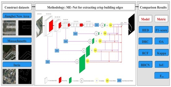
• We constructed the Jiangbei New Area building edge dataset and reconstructed two building edge datasets based on the public Massachusetts and Inria building region datasets; We then re-trained and evaluated the state-of-the-art DCNNs-based edge detection networks (HED, DRC, RCF, and BDCN) on the three large building edge datasets of very high resolution remote sensing imagery;
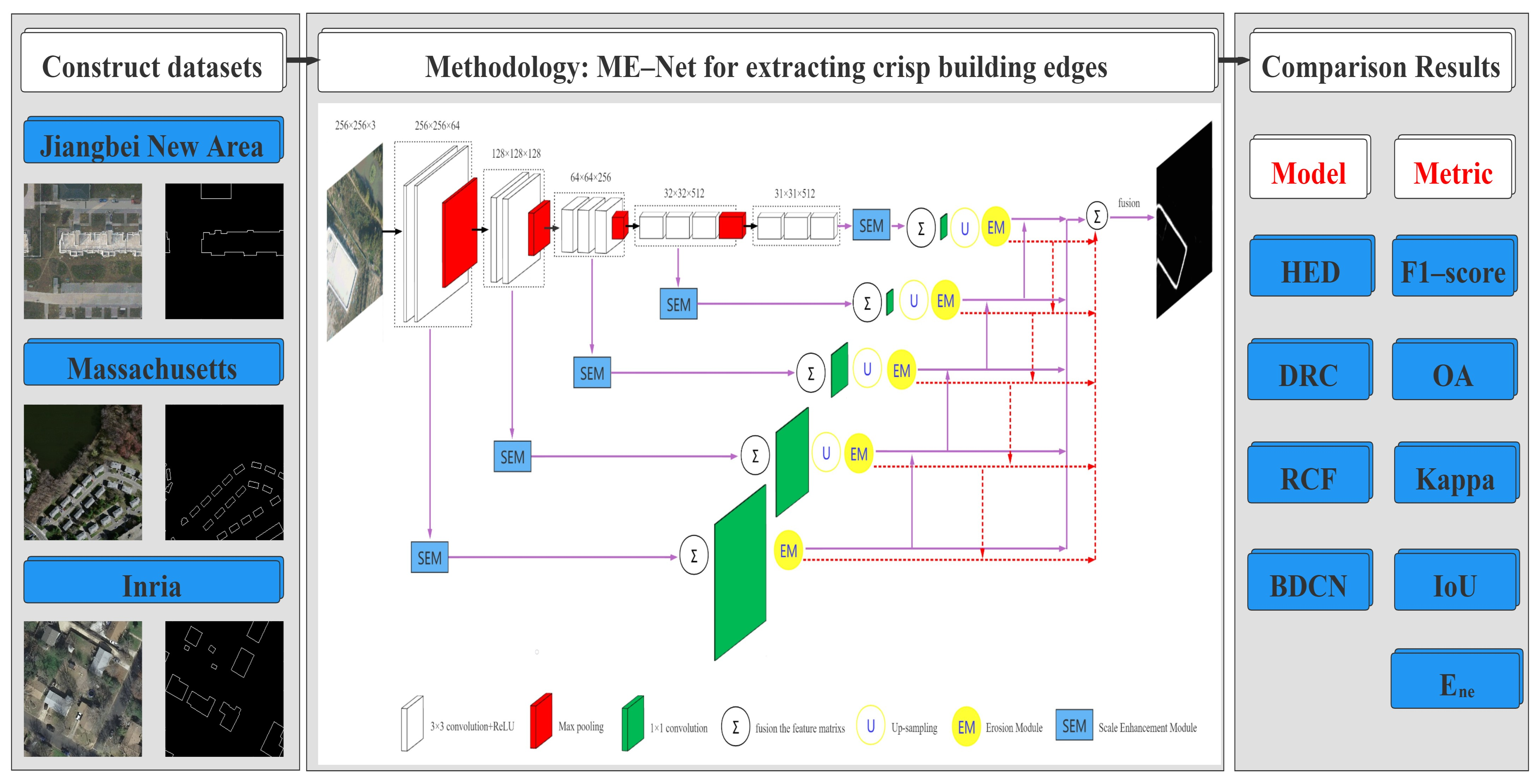
• Based on the architecture of BDCN, a multi-scale erosion network (ME-Net) was proposed to detect crisp and clear building edges by designing an erosion module (EM) and a new loss function. Compared with the state-of-the-art networks on each dataset, the results demonstrated the universality of the proposed network for building edge extraction tasks;
• We proposed a new metric of non-edge energy (E_ne) to measure the non-edge noise and thick edge, and the metric has shown reliability by exhaustive experiments and visualization results of crisp edges.

The remainder of this paper is organized as follows. In Section 2, the dataset and pre-processing are introduced in detail. Section 3 illustrates the architecture of the proposed ME-Net and explains the composition and function of each module. In Section 4, the results of the four networks and our ME-Net are compared. Discussion and conclusions regarding our study are presented in Section 5 and Section 6, respectively.

2. Dataset Construction

For training deep neural networks, it is necessary to construct building edge datasets with quantities of labeled benchmarks. In recent years, semantic segmentation networks have shown significant classification capabilities on different building region datasets, including the Massachusetts dataset [9,43,44] and the Inria dataset [9,12,45,46]. The two datasets consist of original high-resolution remote sensing images and building region maps, and we need to convert the building region maps to building edge maps for training building edge detection networks. In addition, Jiangbei New Area, Nanjing City, Jiangsu Province, China, is included as the study area in this paper. We constructed the Jiangbei New Area building edge dataset through the visual interpretation of the unmanned aerial vehicle (UAV) aerial image.

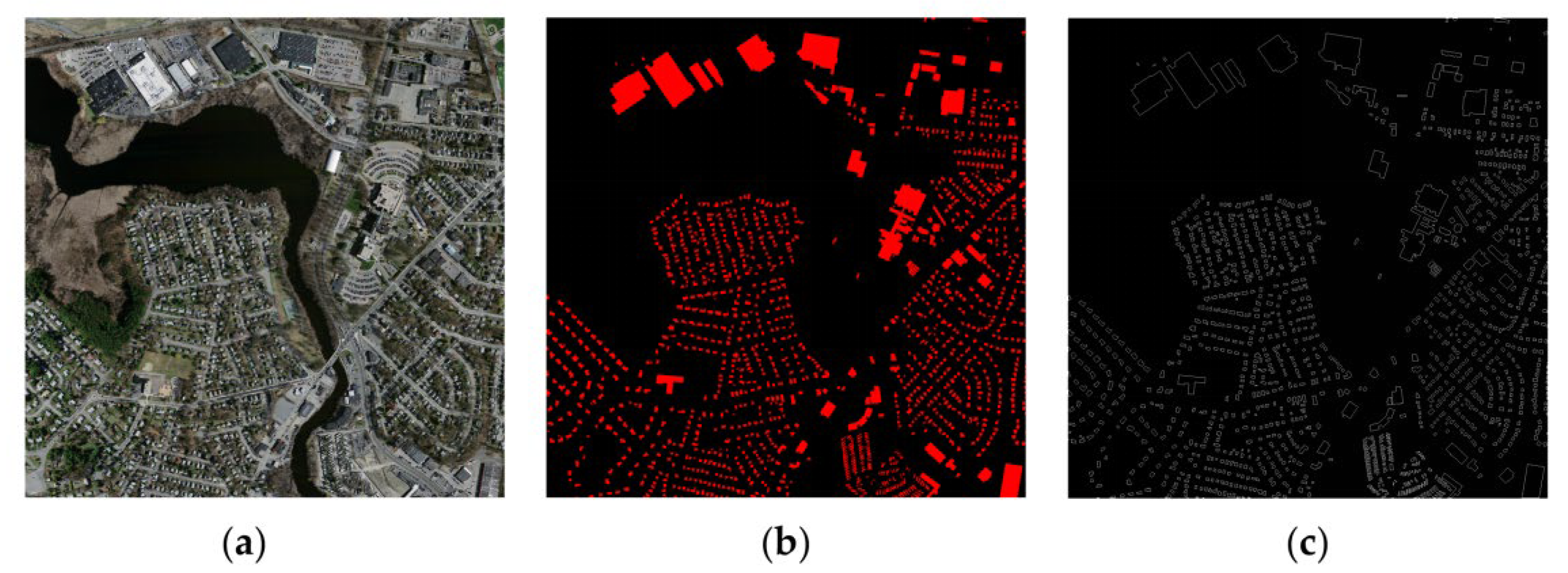
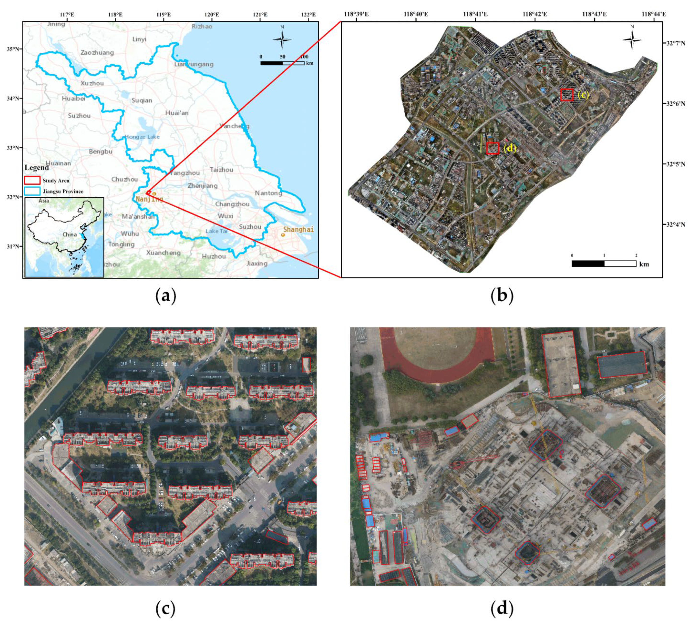
2.1. Jiangbei New Area Building Dataset

This dataset is based on digital orthophoto imagery from aerial photography of unmanned aerial vehicles in the Jiangbei New Area in October 2019. As shown in Figure 1, the entire area covers 53.67 km² with a size of 27,337 × 21,816 pixels (0.3 m ground resolution) and contains 7602 independent buildings. The benchmarks were labeled by manual visual interpretation and were highly accurate. The construction of this building edge dataset is composed of the following three steps:

(1)

The manually vectorized building edge maps were converted to raster binary label images;

(2)

To avoid memory overflow caused by large images, the original aerial images and label images were cropped into patches of 256 × 256 pixels;

(3)

The patches containing buildings were augmented by rotating them 90°, 180°, and 270°.

The final number of patches in the training, validation, and test sets were 8000, 100, and 106, respectively.

2.2. Massachusetts Building Dataset

The Massachusetts Buildings Dataset [43] is an aerial image building dataset marked by the University of Toronto in 2013. As shown in Figure 2a, this dataset covers 364.5 km² with 151 images of 1500 × 1500 pixels each. The ground resolution of this dataset is 1 m, which is lower than that of the Jiangbei New Area building dataset. Therefore, we used this dataset to compare the network performance of the processing of blurred images in high-resolution images.

As shown in Figure 2b, the original building regions label was obtained by rasterizing the high quality building footprints obtained from the Boston OpenStreetMap project, and it includes two classes: building (red) and background (black). To obtain the building edges label, we use a function of Bwperim in MATLAB, which can return a binary image that only contains the perimeter pixels of objects in the input image; a pixel is part of the perimeter if it is nonzero and it is connected to at least one zero-valued pixel [47]. The perimeter pixel of building regions label is building edge pixel, so this function can be used to covert building regions label into building edges label, and the building edges label is shown in Figure 2c.

After conversion, the aerial images and building edges labels were cropped into patches of 256 × 256 pixels. The training patches were selected without cloud obstruction and augmented by rotating 90°, 180°, and 270°. Finally, the Massachusetts building edges dataset is divided into training, validation, and test sets with sizes of 10,500, 100, and 250 patches.

2.3. Inria Building Dataset

The Inria Aerial Image Labeling dataset was proposed in [45]. The Inria dataset covers a large area of 810 km² in 10 cities and contains 360 aerial orthophoto images with a spatial resolution of 0.3 m. As shown in Figure 3a,b, each image has a size of 5000 × 5000 pixels, and each label contains two semantic categories: building and non-building regions. The urban landscape of this dataset is distributed from developed cities with dense populations to mountainous towns, which is valuable for analyzing the generalization ability of different networks.

This dataset only releases the building regions labels of 180 images in the training set, so we followed the suggestions of [9,11,45] and selected the first five original images of each city for testing. The measure to convert this building segmentation dataset is the same as the Massachusetts dataset, and the enlargement sample of the building edges label is shown in Figure 3f. Notably, because the Inria dataset has sufficient training samples, data augmentation is not performed. Eventually, 55,955 training patches and 9025 test patches were generated in the Inria building edge dataset for the experiment preparation.

3. Methodology

In this study, we followed the scale enhancement module (SEM) and bi-directional cascade transmission of BDCN [36], and designed a multi-scale erosion network (ME-Net) to extract crisp building edges by adding the erosion module to the network and constructing a loss function for edge thinning.

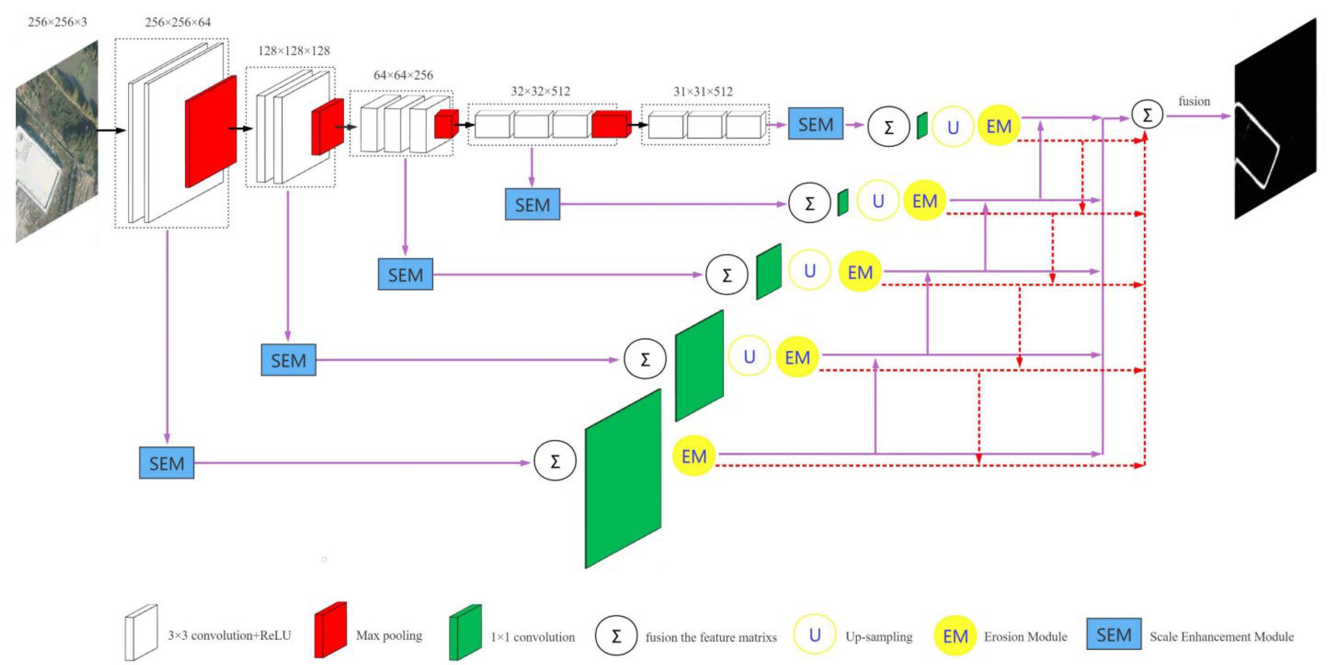
3.1. Architecture Overview

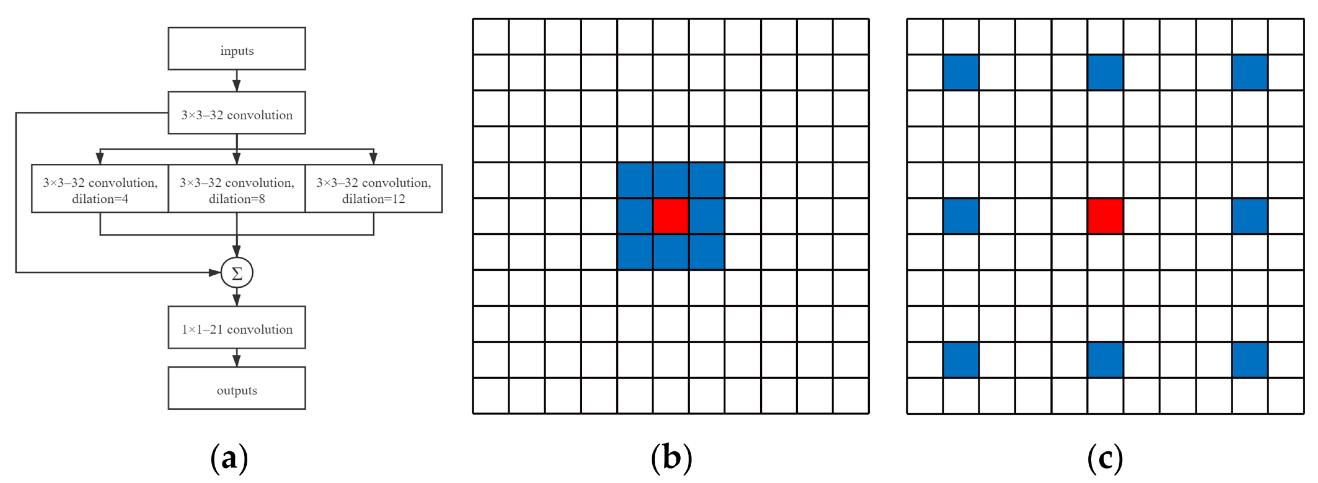
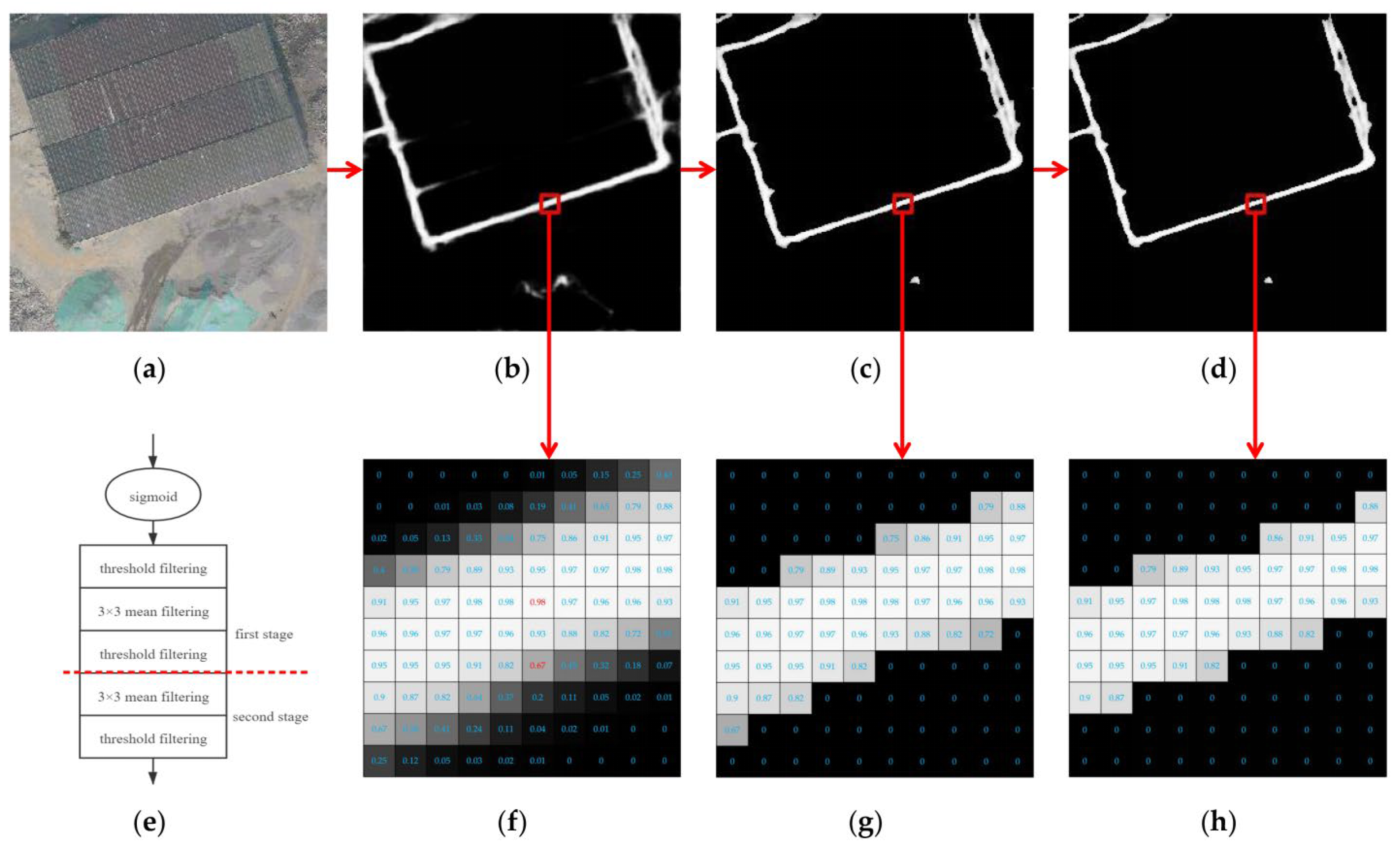
ME-Net is proposed as an end-to-end network that extracts building edge pixels from input high-resolution images. The backbone is VGG16 [48], because the fully connected layers greatly reduced the efficiency of training and the last pooling layer produced a too fuzzy building edge prediction map, so the three fully connected layers and the last pooling layer of VGG16 are removed. The network architecture is illustrated in Figure 4. ME-Net consists of five similar side layers, and each side layer includes several consecutive steps: first, the convolution layer and the maxpooling layer for extracting image features (input: original image; output: image feature map); second, the scale enhancement module (SEM) for extracting multi-scale edge features with the least parameters (input: image feature map; output: building edge feature map); third, the upsampling block for improving the resolution of feature map (input: building edge feature map; output: building edge feature map); last, the erosion module (EM) for crisping the building edge pixels (input: building edge feature map; output: building edge probability map).

Different sizes of building edges cannot be detected at the same scale, so each side layer of different receptive fields is used to detect edges at different scales. In addition, after the erosion module, we follow the BDCN [36] pathway of bi-directional cascade transmission to enrich building edge features. Each side layer propagates two outputs from its adjacent layers and detects the building edges in an incremental manner. Finally, a total of 10 side layer outputs and one fusion layer output are calculated loss with the label.

To remove small non-building edges, such as chimneys or windows, we have to extract rich multi-scale edge features with the least convolution kernel parameters. Therefore, we set a scale enhancement module (SEM) [36] at each stage, and the details of the SEM are shown in Figure 5a, including a standard 3 × 3–32 convolution layer, three 3 × 3–32 dilated convolution [49] layers with dilations of 4, 8, and 12, respectively. As can be seen in Figure 5b,c, with the same number of parameters, a 3 × 3 dilated convolution kernel with dilations of 4 expands the receptive field from 3 × 3 to 9 × 9, and extracts deep edge information at a large scale.

3.2. Erosion Module

Erosion (usually represented by ⊖) [50] is one of two basic operators (the other being dilation) in mathematical morphology, and it can be used for binary or grayscale images. The function of erosion for grayscale images may be expressed as follows:

$$(f\ominus b)(x)=\underset{y\in B}{inf}[f(x+y)-b(y)]$$

(1)

where f(x) denotes the grayscale image to be erode, b(x) denotes the grayscale structuring element, and ”inf” denotes the infimum.

Following the idea of erosion, this study designed an erosion algorithm to crisp the edge probability map. Figure 6f shows the probability map of an enlarged edge segment with a width of nearly six pixels. It can be seen that the probability value is large in the middle and small on both sides of the edge, and it is feasible to weaken the outermost pixel values to refine the edges. Motivated by the mean smoothing operator, we designed an erosion module (EM) with two stages to erode the outermost edge pixels, the details of which are shown in Figure 6e. The EM includes three threshold filtering layers for screening the input building edge probability map and filtering out the edge pixels with the value less than the filter threshold (the filter threshold is set to 0.5). The EM also includes twice repeated mean filtering, that is, for every pixel, the median of neighboring pixels in a 3 × 3 window is calculated, and a value less than the filter threshold is filtered out; this operation is performed twice, and each output is shown in Figure 6c,d. As shown by the red pixels in Figure 6f, the pixel value is 0.98 in the middle and 0.67 in the outermost side; after the mean filtering of the first stage, the pixel value changes to 0.95 in the middle and to 0.47 in the outermost side. It is clear that the center edge pixel with a large probability value is almost unchanged, whereas the outermost edge pixel with a small probability value is weakened.

In this study, the EM is placed at the tail end of each side layer in ME-Net. Thus, each side layer can not only monitor the edge characteristics of different scales, but also generate accurate and crisp building edges after fusion.

3.3. The Proposed Loss Function for Crisp Edge Detection

The loss function, also known as the cost function, aims to minimize the difference between the prediction and ground truth. Generally, very high resolution aerial imagery contains complex ground objects, such as buildings, roads, playgrounds, and trees. The effective loss function can not only suppress non-building edge information interference but also predict crisp building edges.

The building edge extraction can be regarded as the binary classification of pixels, and the most commonly used loss function is binary cross entropy (BCE). However, unlike the issue of image classification or image segmentation, the number of edges/non-edges is imbalanced, and the BCE loss function will lead the training model to focus on the category with a large number of samples, whereas the model will ignore the category with a small number of samples; thus, the generalization ability of the model on the test data will be affected. HED [33], RCF [34] and BDCN [36] used weighted binary cross entropy instead, which has the form:

$$L_{weighted-BCE}=-\frac{\left|Y_{-}\right|}{\left|Y\right|}{\displaystyle \sum _{i\in Y_{+}}\cdot p_i\cdot log(g_i)}-\frac{\left|Y_{+}\right|}{\left|Y\right|}\cdot balance{\displaystyle \sum _{i\in Y_{-}}(1-p_i)\cdot log(1-g_i)}$$

(2)

where p_i and g_i denote the value of the i-th pixel in the prediction result and the ground truth label, respectively. Y₊, Y₋, and Y denote the edge sample set, non-edge sample set, and total sample set in the label, respectively. Balance is the balance coefficient with a default value of 1.1.

Although the weighted binary cross entropy offsets the imbalance between edges and non-edges in edge detection [33], the “thickness” problem remains unsolved. Another approach to solving the issue of edge thickness employs the Dice coefficient. VNet [51] first validated the effectiveness of Dice loss, which was later widely used in medical image segmentation. Following this idea, LPCB [41] proposed a new loss function (L_d), allowing for the generation of crisp edges, and the training process is more stable than Dice loss. L_d is given by the following equation:

$$L_d=\frac{{\displaystyle {\sum }_i^N{p}_i^2}+{\displaystyle {\sum }_i^N{g}_i^2}}{2{\displaystyle {\sum }_i^N{p}_i{g}_i}}$$

(3)

where p_i and g_i denote the value of the i-th pixel in the prediction result and the ground truth label, respectively.

The above work obtains a relatively fine edge; in fact, there is still great space for improvement. Large receptive fields can lead to similar responses of neighboring pixels and lead to thick edges, which means that the loss function is not sensitive enough near the edge. Therefore, we enhance the sensitivity of the loss function near the edge by adding a function that focuses on the loss near the edge pixel. We call it L_local, which is the weighted cross entropy in the eight neighborhoods of label edge pixels, focusing on suppressing the error prediction of thick edges within the local range of positive samples in the label. L_local can be expressed as:

$$L_{local}=-\frac{\left|Y_{local-}\right|}{\left|Y_{local}\right|}{\displaystyle \sum _{i\in Y_{+}}\cdot p_i\cdot log(g_i)}-\frac{\left|Y_{+}\right|}{\left|Y_{local}\right|}\cdot balance{\displaystyle \sum _{i\in Y_{local-}}(1-p_i)\cdot log(1-g_i)}$$

(4)

where Y_local− and Y_local denote the non-edge sample set and total sample set in the eight neighborhoods of the edge sample in the label, respectively.

To achieve better performance, we proposed combining the three loss functions above by setting the corresponding hyperparameter. This can not only compare the prediction and ground truth but also minimize their distance on the datasets. As a result, we calculated the total loss of each side layer as well as the fusion layer and applied it to the network. The final loss function is given by:

$$L_{final}(P,G)=\partial L_{weighted-BCE}^{side+fusion}(P,G)+\beta L_d^{fusion}(P,G)+\gamma L_{local}^{fusion}(P,G)$$

(5)

where P and G represent the prediction map and the ground truth label, respectively, and α, β, and γ are the hyperparameters controlling the influence of the three losses. We tuned the parameters as α = 1, β = 10, and γ = 1 with high accuracy.

3.4. Evaluation Metrics

Normally, six metrics are used to measure the effect of edge extraction: overall accuracy (OA), precision, recall, F1-score (F1), intersection over union (IoU), and kappa coefficients (Kappa):

$$Precision=\frac{TP}{TP+FP}.$$

(6)

$$Recall=\frac{TP}{TP+FN}.$$

(7)

$$F_1=\frac{2\ast Precision\ast Recall}{Precision+Recall}.$$

(8)

$$OA=\frac{TP+TN}{TP+FP+TN+FN}.$$

(9)

$$IoU=\frac{TP}{TP+FP+FN}.$$

(10)

$$Kappa=\frac{p_0-p_e}{1-p_e}.$$

(11)

$$p_0=\frac{TP+TN}{N}.$$

(12)

$$p_e=\frac{(TP+FP)\ast (FN+TP)+(TN+FN)\ast (FP+TN)}{N^2}.$$

(13)

where N, TP, FP, TN, and FN represent the total samples and the true positive, false positive, true negative, and false negative predictions, respectively. p₀ and p_e represent the consistency rate in prediction and consistency rate, respectively, in expectation.

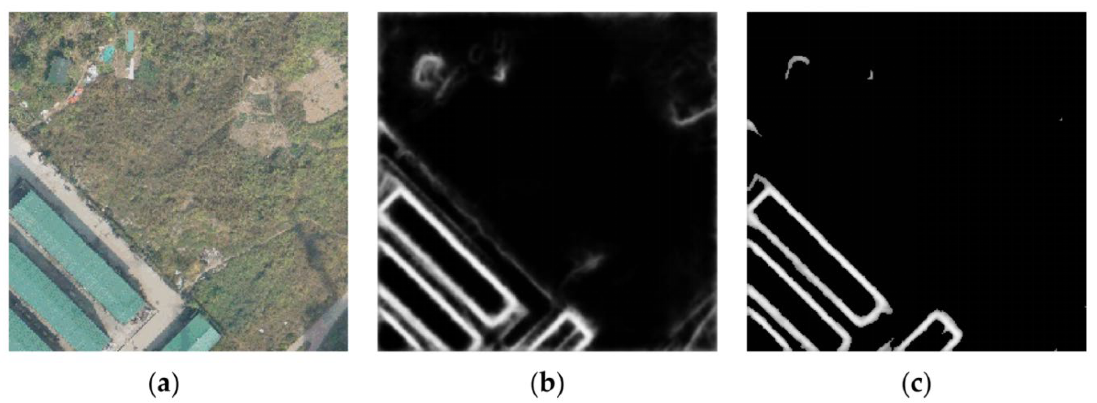
3.5. The Proposed E_ne for Edge Crispness Measuring

Among the above metrics, the F1-score is the most important because it is the harmonic mean of the precision and recall. In edge detection by convolutional neural networks, the result is a probability map with values between 0 and 1; it is necessary to set a threshold (after this, called Th) of transforming the probability map into a binary map [52,53,54] larger than Th for edge pixels, and Th is typically 0.5 [44]. Based on the edge pixels and non-edge pixels, the number of positive and negative samples may be calculated, and the F1-score may be achieved. However, the F1-score cannot measure the quality of edge probability map entirely. If there are two edge probability maps in which the pixels larger than the Th are the same, and the pixels smaller than the Th are different, then, the F1-score is the same. As shown in Figure 7b,c, the left edge probability prediction is messier and thicker than that on the right, but they achieved the same strict F1-score of 35.40%. This means that the F1-score can only measure the quality of the part larger than Th in the edge probability map and cover up the thickness issue of the edge. Therefore, we need an index to measure the quality of a part with values less than a threshold in the edge probability map.

We propose a new indicator called non-edge energy (E_ne), which can measure the quality of a part with values less than the threshold of calculating E_ne in the edge probability map effectively, which can be expressed as:

$$E_{ne}=\frac{{\displaystyle \sum P_i}}{N}/T.$$

(14)

where T denotes the threshold of calculating E_ne (default is 0.5), P_i denotes the probability value of the i-th pixel that is less than T, and N denotes the number of pixels with probability values less than T.

E_ne can be understood as the even energy of non-edge pixels in the edge probability map; the smaller the value, the smaller the non-edge noise. It also can reflect the edge quality of human vision well, that is, whether or not the edge probability map is neat.

4. Experiments and Results

We test the edge detection of the proposed ME-Net based on three datasets and compare the results with other state-of-the-art networks using the metrics described in Section 3.4. There are two schemes for calculating metrics: strict and relaxed [55]. Mnih et al. [43] introduced relaxed precision and relaxed recall as practical metrics for hard-labeling datasets. The relaxed precision is defined as the fraction of predicted building edge pixels that are within ρ pixels of a true building edge pixel, whereas relaxed recall is defined as the fraction of true building edge pixels within the ρ pixels of a predicted building edge pixel [56]. Generally, the relaxation parameter ρ was set to 3 [43,57] for all experiments discussed in this study.

4.1. Training Details

We implemented all the networks using PyTorch1.4.0 and Pytorchvision0.5.0, with CUDA 9.2. All the experiments were conducted on an NVIDIA Quadro P4000 GPU with 16 GB of memory. We set iterations equal to the number of training data and adopt the SGD optimizer to train our network. The initial learning rate, momentum, weight decay, batch size, epoch of four datasets, training time of four datasets, step size of decreasing learning rate, and model parameters are listed in

Table 1. Hyperparameters and time of training DCNNs-based edge detection models on Jiangbei, Massachusetts, Inria and BSDS500 ¹ datasets.

Model	HED	RCF	BDCN	DRC	ME-Net
Learning rate	1e-6	1e-6	1e-6	1e-3	1e-6
Momentum	0.9	0.9	0.9	0.9	0.9
Weight decay	0.002	0.002	0.002	0.002	0.002
Batch size	10	10	1	1	1
Epoch	30, 30, 10, 10	30, 30, 10, 10	30, 30, 10, 10	8, 8, 4,8	30, 30, 10, -
Step size (proportion)	1/3	1/3	1/4	1/4	1/4
Parameter	14,716,171	14,803,781	16,302,712	32,336,202	16,302,925
Training Time (h)	5.5, 7.5, 10.8, 9.8	39.0, 16.5, 28.3, 31.8	61.0, 29.6, 51.0, 57.0	26.6, 18.4, 63.7, 97.6	43.5, 31.1, 42.5, -

¹ The results on BSDS500 dataset will be shown in Section 5.1.

. Notably, although the training iterations may be slightly different from the published setting of the paper, we ensure that the loss does not decreases and the network converges, so this does not affect the comparison between the performance of networks.

4.2. Comparison Experiments

In this study, we need to set three kinds of thresholds for training the ME-Net and calculating the evaluation metrics: the first is the filter threshold in the erosion module in Section 3.2, the second is the threshold of transforming the building edge probability map into a building edge binary map in Section 3.5, the third is the threshold of calculating E_ne metric in Section 3.5. Considering the efficiency of training and the uniformity of calculating metrics, all the thresholds are set to 0.5.

In order to compare our proposed ME-Net with the state-of-the-art edge detection networks comprehensively, we show the comparison results of evaluation metrics and building edge probability maps on the Jiangbei New Area dataset in Section 4.2.1, Massachusetts Dataset in Section 4.2.2, and Inria Dataset in Section 4.2.3.

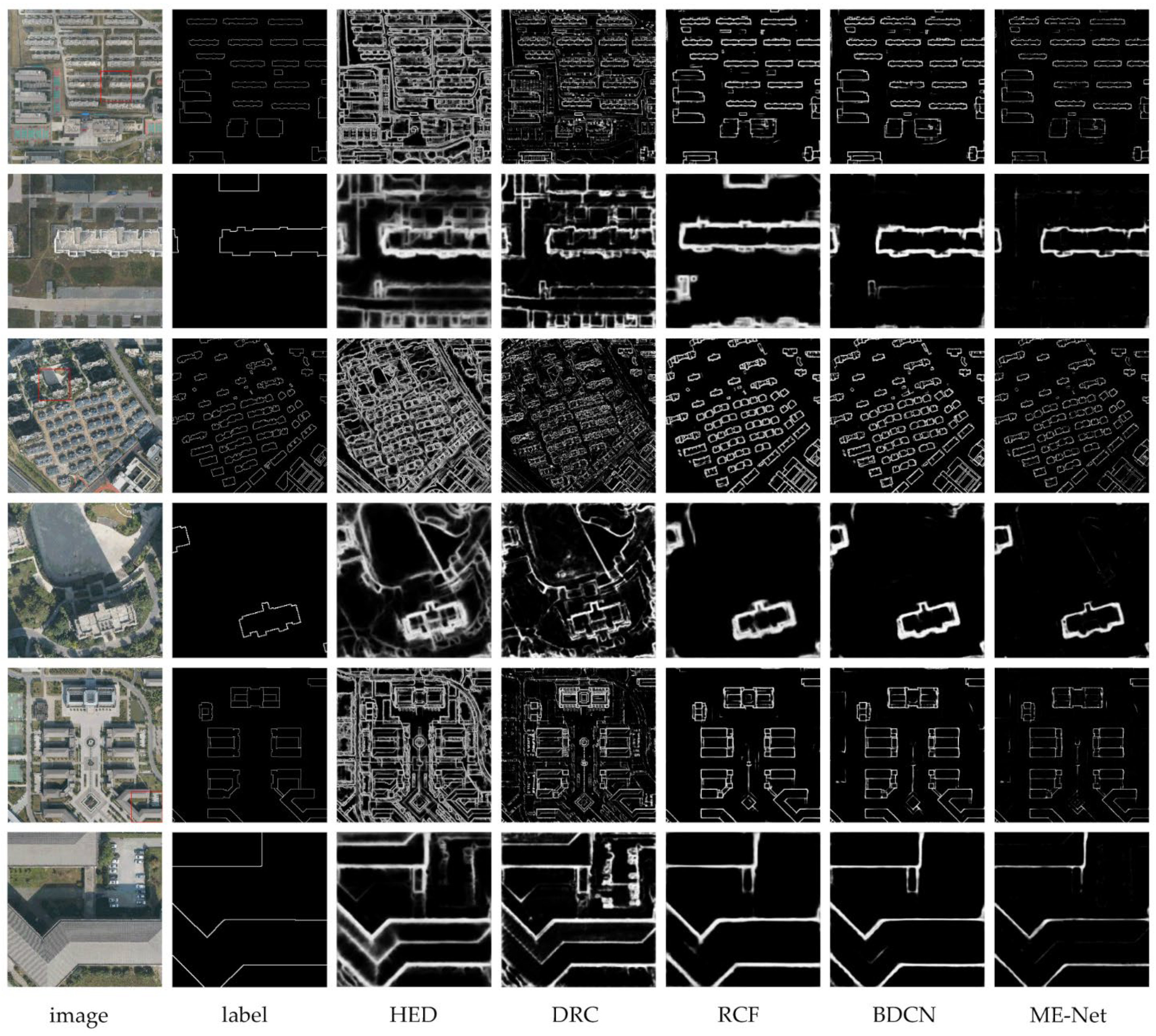
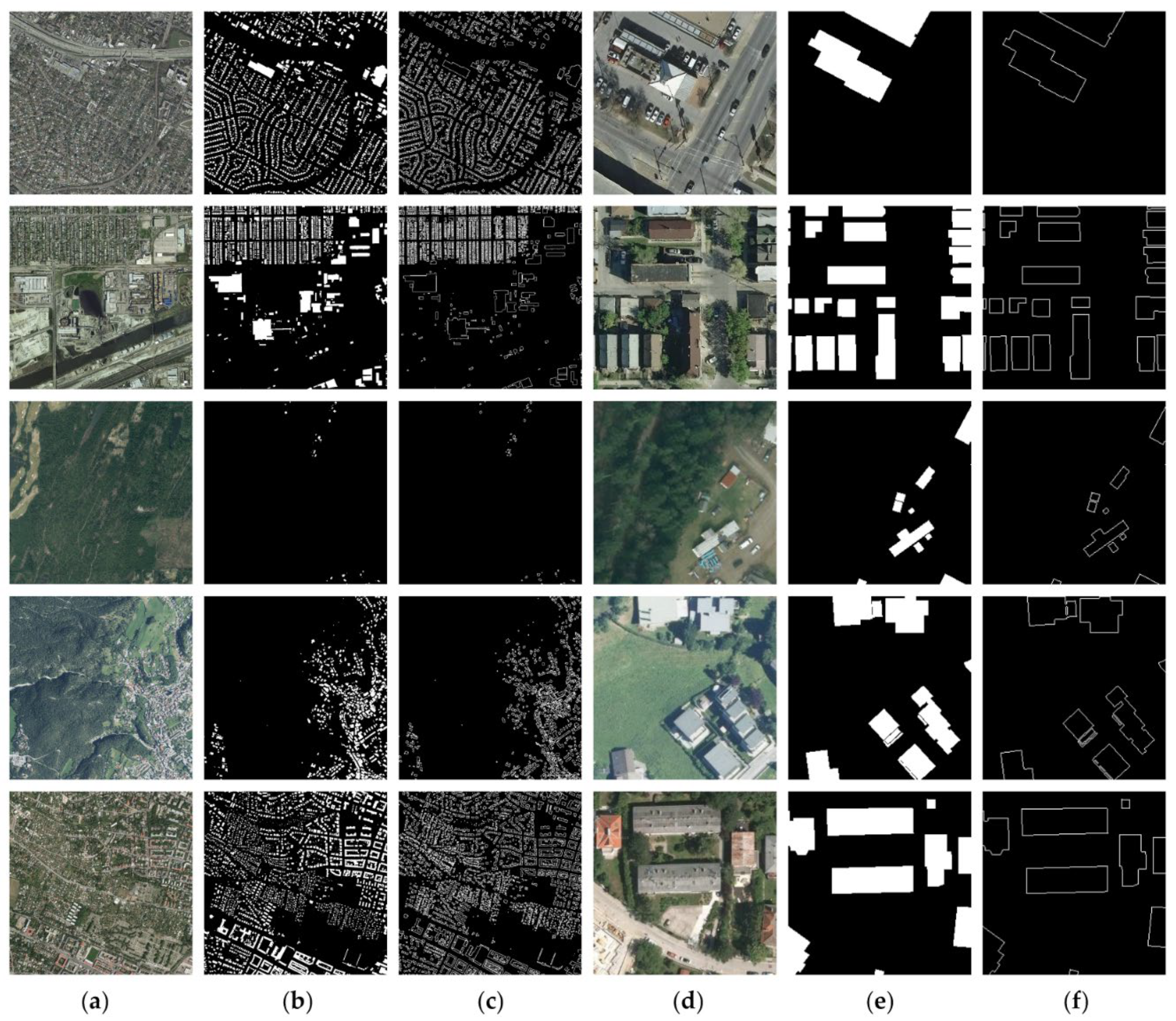
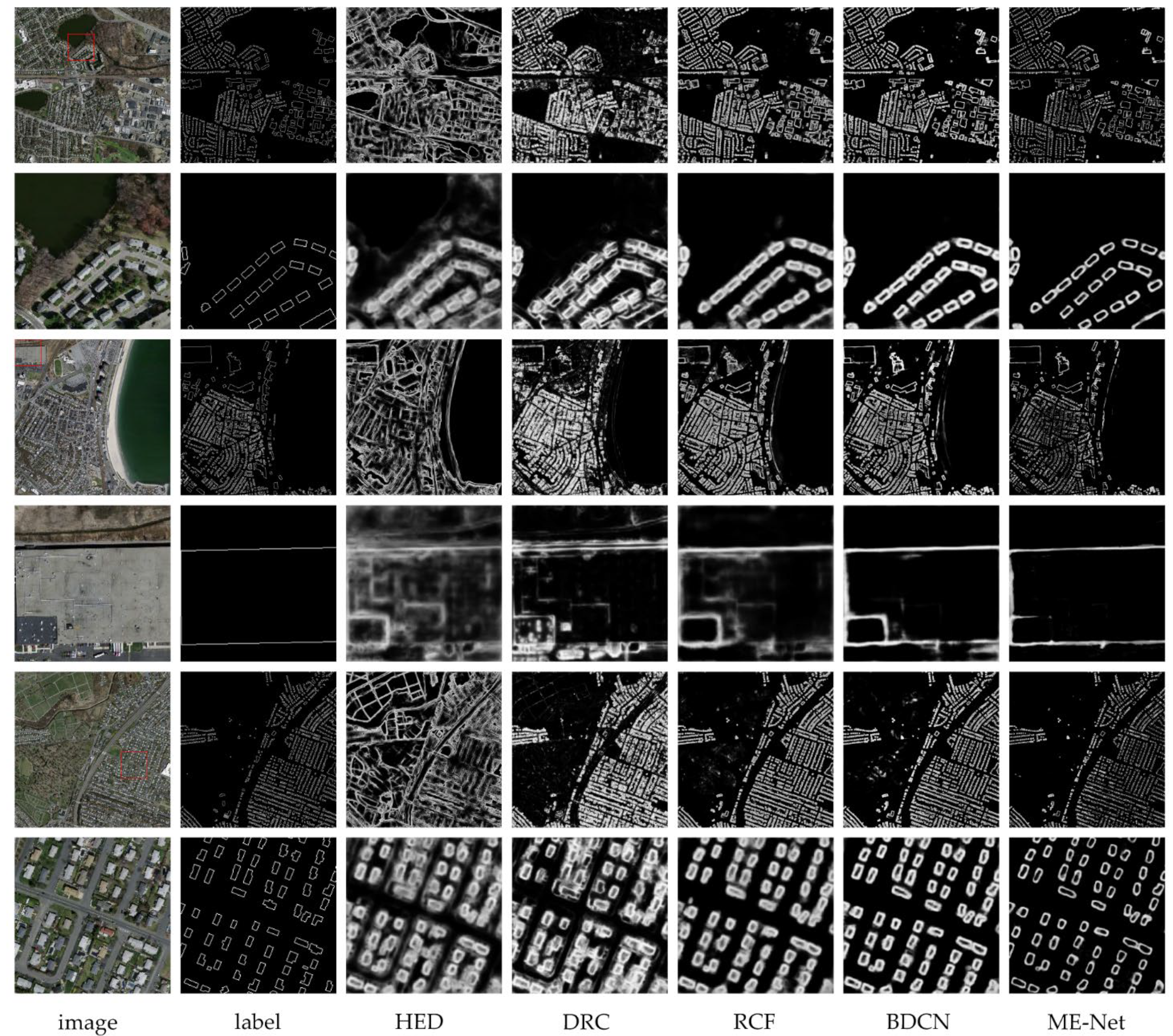
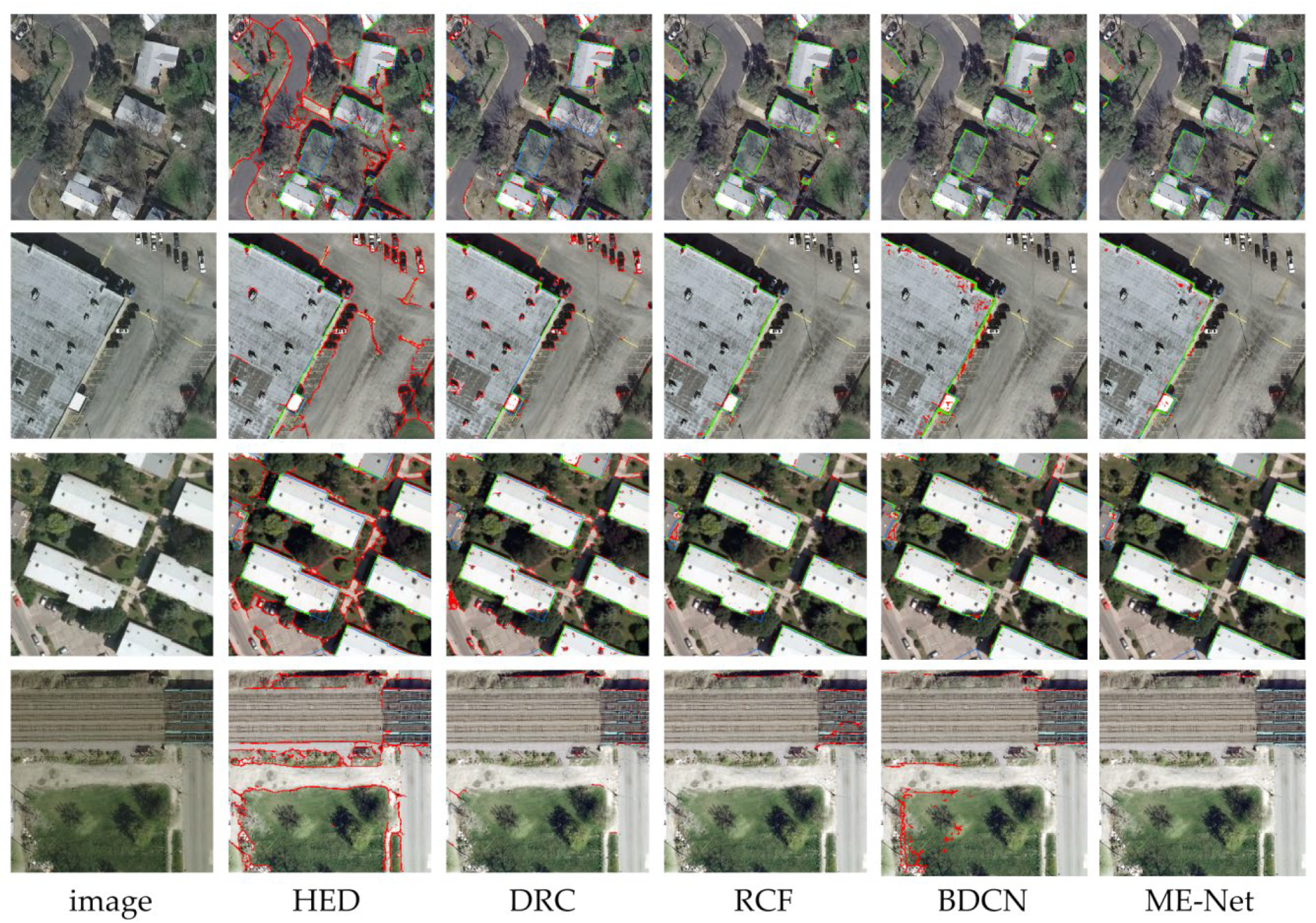
4.2.1. Results on Jiangbei New Area Dataset

We trained HED, RCF, BDCN, DRC, and ME-Net and evaluated the metrics on the Jiangbei New Area dataset.

Table 2. Evaluation results on the test set of Jiangbei New Area dataset. Each cell has the value with strict and relaxed metrics and the best values are masked as bold (the lowest E_ne indicates the clearest and crispest result).

Model	Scheme	OA (%)	F1 (%)	Precision (%)	Recall (%)	Kappa (%)	IoU (%)	Ene (%)
HED	strict relaxed	87.99, 90.28	17.08, 41.82	9.38, 26.78	95.31, 95.40	15.08, 38.63	9.34, 26.66	18.74
DRC	strict relaxed	91.56, 92.91	17.11, 36.90	9.80, 24.98	67.06, 70.54	15.18, 35.88	9.35, 23.84	10.80
RCF	strict relaxed	93.99, 96.25	29.07, 64.38	17.17, 48.71	94.84, 94.92	27.48, 63.36	17.01, 48.26	3.84
BDCN	strict relaxed	95.07, 97.20	33.42, 69.84	20.26, 55.11	95.21, 95.30	31.96, 69.25	20.06, 54.55	2.42
ME-Net	strict relaxed	97.34, 98.75	44.58, 76.89	30.54, 70.73	82.50, 84.21	43.51, 79.19	28.68, 66.43	1.98

lists the strict and relaxed quantitative evaluation metrics of the different models on the test set. The strict OA of all networks remained above 87%, and our ME-Net exceeded 97%. Evidently, ME-Net is superior to HED, DRC, RCF, and BDCN in all seven metrics, except for the recall index. This can be explained by the prediction of the crispest building edge, where the edges become thinner, the number of false positive samples decreases obviously, but the number of false negative samples increases at the same time, leading to a lower recall index. However, ME-Net achieves the best balance between precision and recall, as can be seen from the highest F1-score. The E_ne is lower than 4% in the predictions of RCF and BDCN, and ME-Net achieves the minimum value of 1.98%, which means that our proposed network has the best constraint ability on non-edge noise and thick edges. Moreover, compared with the results of BDCN, our ME-Net improved by 1.55%, 7.05%, 9.94%, and 11.88% in relaxed OA, F1, Kappa, and IoU, respectively.

Figure 8 shows three different cases of building edge probability maps in the test dataset. The odd rows are test images and results with size of 1280 × 1280 pixels, and the even rows are patches of 256 × 256 pixels in the selected areas by red boxes. The first case compared the detection of large building edges from a school. HED and DRC could not distinguish the building edge from the noisy edge. BDCN and ME-Net extracted a clearer edge but missed a small part of it. The second case was used to show the edge detection of small and dense residential buildings, compared with other networks, ME-Net had the least false predictions. The last case was an edge detection of large office buildings. RCF and BDCN performed better than HED and RCF with fewer negative roof edges, and only ME-Net could predict all building edges, which almost matches the label. In short, our ME-Net has the best performance with the most regular building edge shape and the crispest edge.

4.2.2. Results on Massachusetts Dataset

In the Massachusetts building edge dataset, we evaluated 250 test images with a size of 256 × 256 pixels.

Table 3. Evaluation results on Massachusetts test set. Each cell has the value with strict and relaxed metrics and the best values are masked as bold for columns 3–8. The last column is E_ne, and the lowest value indicates the clearest and crispest result.

Model	Scheme	OA (%)	F1 (%)	Precision (%)	Recall (%)	Kappa (%)	IoU (%)	Ene (%)
HED	strict relaxed	74.61, 82.24	19.31, 53.07	10.87, 38.17	86.19, 87.03	13.92, 45.95	10.69, 37.52	37.90
DRC	strict relaxed	74.18, 80.99	17.28, 47.78	9.74, 34.35	76.52, 78.45	11.76, 41.16	9.46, 33.35	24.56
RCF	strict relaxed	79.66, 87.39	23.48, 61.59	13.54, 47.05	88.54, 89.17	18.50, 56.68	13.30, 46.24	19.38
BDCN	strict relaxed	82.24, 89.72	25.82, 65.32	15.14, 51.77	87.69, 88.48	21.08, 61.82	14.83, 50.69	11.94
ME-Net	strict relaxed	90.99, 95.00	28.99, 62.69	20.07, 63.81	52.19, 61.61	25.18, 67.35	16.95, 53.91	5.78

lists the strict and relaxed quantitative evaluation metrics of different models on the test set. Compared with Table 2, all the metrics of the five networks decreased significantly because of the lower resolution in this dataset. Note that our proposed ME-Net (95.00%) outperformed the HED (82.24%), DRC (80.99%), RCF (87.39%), and BDCN (89.72%) in terms of relaxed OA, with a minimum increase of 5.28%. Compared with the other four networks, despite having the lowest recall, our proposed ME-Net with strict F1-score, precision, kappa, and IoU increased by 7.52%, 7.75%, 8.87%, and 4.88% on average, respectively. Although our network is slightly inferior to BDCN in terms of relaxed F1-score, we predict clearer and more acceptable building edges with nearly half the E_ne than BDCN.

Similar to Figure 8 and Figure 9 presents some building edge probability map samples of Massachusetts test images. The odd rows are the original test images with a size of 1500 × 1500 pixels, and the even rows are selected as the most common building complex of 256 × 256 pixels in the red boxed areas above. As shown in the first two rows, when detecting building edges near the lake, HED and DRC misclassified the edges of non-buildings and created many noisy results. BDCN delivered a more effective and tidy prediction than RCF, and our ME-Net detected the most accurate and crisp building edge. For large-sized buildings in the 3rd and 4th rows, all networks misjudged the small block on the roof except ME-Net, and BDCN and ME-Net predicted more true positives for the relatively complete boundary prediction. The 5th and 6th rows are densely distributed small-sized buildings, although ME-Net did not achieve a one-pixel-width building edge, we predicted the clearest result for the lowest probability values of non-buildings. Compared with the state-of-the-art DCNNs-based edge detection networks, we predicted the best results in distinct buildings of the Massachusetts dataset.

4.2.3. Results on Inria Dataset

In the Inria dataset, we evaluated 9025 test images with a size of 256 × 256 pixels.

Table 4. Evaluation results on the test set of Inria dataset. Each cell has the value with strict and relaxed metrics and the best values are masked as bold (the lowest E_ne indicates the clearest and crispest result).

Model	Scheme	OA (%)	F1 (%)	Precision (%)	Recall (%)	Kappa (%)	IoU (%)	Ene (%)
HED	strict relaxed	81.29, 82.64	5.63, 17.42	2.96, 10.15	57.05, 61.35	3.84, 14.52	2.89, 9.93	25.10
DRC	strict relaxed	89.86, 90.89	7.99, 22.77	4.38, 14.67	45.02, 50.84	6.32, 21.82	4.16, 13.92	19.24
RCF	strict relaxed	89.61, 91.57	13.34, 38.51	7.26, 25.10	81.81, 82.70	11.76, 36.67	7.15, 24.70	19.20
BDCN	strict relaxed	88.55, 90.61	12.84, 37.49	6.94, 23.91	86.25, 86.85	11.23, 35.09	6.86, 23.64	15.84
ME-Net	strict relaxed	94.00, 95.51	17.49, 45.52	10.11, 34.03	65.01, 68.75	16.07, 46.91	9.58, 32.27	3.32

lists the strict and relaxed quantitative evaluation metrics of different models on the test set. The Inria dataset covers the largest areas and most complicated types of cities, resulting in the lowest label quality and accuracy. Nevertheless, ME-Net achieves the best results with a relaxed OA of 95.51% and F1-score of 45.52%, which are observably higher than the four comparable networks. In addition, our network achieves the highest Kappa and IoU for the entire test set, meaning that our prediction results overlap the most with the real ground truth. Moreover, it was observed that ME-Net outperformed HED, DRC, RCF, and BDCN by 21.78%, 15.92%, 15.88%, and 12.52%, respectively. Similar conclusions can be drawn that the comprehensive ability of ME-Net in this dataset is the best.

Considering the similarity of urban settlements, we show the building edge probability map of the representative test images from three cities in Figure 10. The odd rows are the original test images with a size of 5000 × 5000 pixels in Austin, Kitsap, and Tyrol, and the even rows are samples of 256 × 256 pixels in the red boxed areas of interest. The buildings in Austin are compact and orderly. Over such a wide area of edge detection, HED produces many false positive predictions that lead to messy results, DRC cannot predict the complete building contours, and ME-Net distinguishes the adjacent buildings most effectively. Kitsap has sparse buildings because it covers a large area of forests, and the irregular building edge extracted by RCF and BDCN is fuzzy, whereas ME-Net can better judge non-building edges and provide clearer edge detection. For buildings of plain areas in Tyrol, the accuracy of label is controversial due to fact that all the networks missed a small indistinguishable building. Besides this, RCF and BDCN misclassified some shadow and ground boundaries as building edges, and our ME-Net detected the cleanest and crispest building edges in different types of cities and towns.

To further explore the improvements in our network compared to other networks, several representative samples from the Inria dataset were selected for additional comparison. Actually, the lineness of edge pixels detected by DCNNs-based edge detection networks can be further crisped, and at present, the non-maximum suppression (NMS) method is the most primary post-process method. Figure 11 shows the detailed edge information generated by different networks after the post-processing of NMS. Considering the inaccuracy of the edge labels, an error of one pixel was allowed. First, for the small-sized buildings and large buildings presented in the first and second samples in Austin, HED and DRC incorrectly predicted many boundaries of roads, trees, and cars as building edges. Compared with RCF and BDCN, ME-Net predicted more true positives (green pixels) and true negatives (background pixels) and detected more complete building edges. Second, for the dense and regular buildings of the third sample in Vienna, ME-Net predicted the fewest false positives (red pixels) and false negatives (blue pixels). The last scene is an entire negative sample containing no buildings in Chicago. Obviously, our ME-Net predicted the most accurate results with few building edges, whereas the other HED, DRC, RCF, and BDCN had more or less false positive predictions. In general, the progression from left to right in each row suggests that our proposed ME-Net performs better than other state-of-the-art DCNNs-based edge detection networks.

5. Discussion

5.1. Reliability Verification of Codes

We compared three datasets between our proposed network and the published networks of HED [33], RCF [34], BDCN [36] and DRC [38]; however, before making this comparison, it is necessary to ensure that the implementation of these networks is correct. Although the source code of these networks has been published, there are still missing of many details in the implementation and training process of the network, including the setting of hyperparameter of initial learning rate, momentum, weight decay, batch size, and iterations. To demonstrate the correctness and reliability of the networks used in this study, we reproduced the source code and training process of these networks based on Pytorch and evaluated their edge detection effect on the BSDS500 dataset [39], and the results are shown in Figure 12, revealing that the edge prediction results of all networks are very close those of the label.

Table 5. Evaluation metrics of our reproduced results and official reported results on the BSDS500 test set.

Model	ODS-F (Ours)	ODS-F (Report)	OIS-F (Ours)	OIS-F (Report)
HED	0.787	0.790	0.804	0.808
DRC	0.789	0.802	0.806	0.818
RCF	0.792	0.806	0.807	0.823
BDCN	0.806	0.806	0.822	0.826

shows evaluation metrics of our reproduced results and official reported results on the BSDS500 test set. Due to the variability of the training process in convolutional neural network, the final evaluation metrics is affected by the number of iterations, the GPU computing power and the different platforms of Pytorch or Caffe. Considering these factors, the ODS-F and OIS-F of our reproduced results are slightly lower than official reported results, but the gap does not exceed 0.02, which illustrated that our reproduced HED, DRC, RCF, and BDCN can be applied to remote sensing building edge datasets.

5.2. Comparative Analysis with Segmentation Methods

As mentioned in the introduction, building region extraction cannot replace edge extraction for two reasons: one is the outline extraction by segmentation networks is often bent and broken [3]; the other is the accuracy of edge converted from building region results normally is lower than that of direct building edge detection.

Kang et al. conducted related experiments using JointNet [44], FastFCN [58], DeepLabv3+ [59] and EU-Net [9], and reported the evaluation results of building mask extraction and indirect building contour detection on the Massachusetts and Inria datasets.

Table 6. Building edge detection results on the Massachusetts test set in terms of F1-score and IoU, the best values are masked as bold.

Model	JointNet (%)	FastFCN (%)	DeepLabv3+ (%)	EU-Net (%)	Our ME-Net (%)
F1-score	27.31	13.73	21.92	28.83	28.99
IoU	15.82	7.37	12.31	16.84	16.95

shows the results of different semantic segmentation networks and our proposed edge detection network on the Massachusetts dataset. It is clear that our proposed ME-Net is superior to the other methods based on F1-score and IoU, proving that ME-Net outperforms the semantic segmentation model in extracting the building edges on the Massachusetts dataset.

Similar to Table 6, we show a statistical comparison of the Inria dataset in

Table 7. Building edge detection results on the Inria test set in terms of F1-score and IoU, the best values are masked as bold.

Model	FastFCN (%)	DeepLabv3+ (%)	EU-Net (%)	Our ME-Net (%)
F1-score	11.18	14.84	20.47	17.49
IoU	5.92	8.01	11.40	9.58

. The results show that our proposed ME-Net achieves a higher IoU than those of FastFCN and DeepLabv3+ at 3.36% and 1.57%, respectively, but lags behind the result from EU-Net by a margin of 1.82%. It is acceptable that ME-Net did not achieve thinning of all edges to one pixel width; thus, it needs to be improved in future work with the Inria dataset.

5.3. Ablation Analysis and Cross-Dataset Evaluation

We designed the erosion module (EM) and the local loss function in our ME-Net. In order to demonstrate the performance and impact of each proposed component, we conducted the ablation analysis of ME-Net against multiple resolution datasets, and the relaxed quantitative evaluation results are shown in

Table 8. Ablation analysis evaluation results of ME-Net, the best values of each dataset are masked as bold.

Dataset	Model	OA (%)	F1-Score (%)	IoU (%)
Jiangbei New Area	ME-Net (remove EM and local loss)	97.20	69.84	54.55
	ME-Net (remove EM)	97.37	70.98	55.91
	ME-Net	98.75	76.89	66.43
Massachusetts	ME-Net (remove EM and local loss)	89.72	65.32	50.69
	ME-Net (remove EM)	89.87	65.63	51.05
	ME-Net	95.00	62.69	53.91
Inria	ME-Net (remove EM and local loss)	90.61	37.49	23.64
	ME-Net (remove EM)	91.14	38.64	24.59
	ME-Net	95.51	45.52	32.27

. On the Massachusetts dataset, although the F1-score of ME-Net is lower than that of ME-Net (remove EM), the ME-Net surpasses the ME-Net (remove EM) 5.13% and 2.86% in terms of relaxed OA and IoU metrics. Meanwhile, on the Jiangbei New Area dataset and Inria dataset, the complete ME-Net achieved the best results in all the three metrics, the ME-Net (remove EM) achieved the second, and the ME-Net (remove EM and local loss) achieved the third, proving that the EM and the local loss are very important for improving the performance of ME-Net.

In the deep learning, a common problem is the transferability of models. In order to clearly describe the transferability of ME-Net, we also conducted the experiment of cross-dataset evaluation. We trained and tested ME-Net with different datasets, and the relaxed quantitative evaluation results are shown in

Table 9. Cross-dataset evaluation results of ME-Net, the best values of each training dataset are masked as bold.

Training Dataset	Testing Dataset	OA (%)	F1-score (%)	IoU (%)
Jiangbei New Area	Jiangbei New Area	98.75	76.89	66.43
	Massachusetts	95.53	20.16	17.87
	Inria	98.03	29.43	23.31
Massachusetts	Jiangbei New Area	98.06	28.21	23.32
	Massachusetts	95.00	62.69	53.91
	Inria	97.46	25.13	19.09
Inria	Jiangbei New Area	95.95	43.20	31.29
	Massachusetts	92.11	40.45	33.04
	Inria	95.51	45.52	32.27

. Obviously, whatever the training datasets, ME-Net achieved the highest relaxed OA on the testing dataset of Jiangbei New Area. In addition, when we trained ME-Net on the Jiangbei New Area dataset and Massachusetts dataset, the relaxed F1-score and IoU of cross-dataset evaluation are greatly inferior to that of training and testing with the same dataset; however, when we trained on the Inria dataset, and test on the three different datasets, the changes of relaxed OA, F1-score, and IoU are lower than 3.84%, 5.07%, and 1.75%, proving that ME-Net achieved the best stability when training on the large-area Inria dataset.

6. Conclusions

In this study, we systematically analyzed the effects of state-of-the-art DCNNs-based edge detection networks (HED, RCF, BDCN, and DRC) on large-scale VHR remote sensing building edge datasets. We found that although these networks have achieved remarkable performance in natural image edge detection, there is still the problem of edge thickness when they are applied to building edge detection from VHR remote sensing images, but BDCN achieved the highest accuracy. Based on the architecture of BDCN, we proposed a novel multi-scale erosion network (ME-Net) to detect crisp building edges. The ME-Net refines the edge through two mechanisms: one is an embedded erosion module to erode the pixels at the outermost edge, and the other is through constructing a multi-objective loss function, including global cross entropy, Dice coefficient, and edge local cross entropy, to increase the sensitivity of the loss function at the building edge pixels. In order to fully verify and compare the effectiveness of the edge detection networks, this study constructs three large-area building edge datasets, including the Jiangbei New Area building edge dataset, Massachusetts, and Inria datasets, and our proposed ME-Net achieves the best edge detection performance on the three datasets. Moreover, we proposed a new metric, E_ne, to measure the non-edge noise and crispness of building edges, which represents the energy of non-edge information in the edge prediction probability map and can reveal the neat and tidy degree of the edge probability map. In order to make it more visible for users to see the lines as they zoom in the image, we have made a video as a Supplemental Materials for overlaying the lineness of building edge pixels on the original image at a higher resolution.

Although our work enhances the crispness of building edge detection, the edge width still does not reach the industry standard required by surveying and mapping applications. The primary reason is that the network based on DCNNs normally has large receptive fields, owing to the multiple convolution and pooling operations, leading to the close loss responses of the pixels near the edge. One possible way to resolve this problem in the future is to construct a network with sufficient depth and a small receptive field, or design a building edge vectorization algorithm to post-process the lineness of the edge pixels.

References

1. Du, S.; Luo, L.; Cao, K.; Shu, M. Extracting building patterns with multilevel graph partition and building grouping. ISPRS J. Photogramm. Remote Sens. 2016, 122, 81–96. [Google Scholar] [CrossRef]
2. Siddiqui, F.U.; Teng, S.W.; Awrangjeb, M.; Lu, G. A robust gradient based method for building extraction from LiDAR and photogrammetric imagery. Sensors 2016, 16, 1110. [Google Scholar] [CrossRef] [PubMed] [Green Version]
3. Wu, G.; Guo, Z.; Shi, X.; Chen, Q.; Xu, Y.; Shibasaki, R.; Shao, X. A boundary regulated network for accurate roof segmentation and outline extraction. Remote Sens. 2018, 10, 1195. [Google Scholar] [CrossRef] [Green Version]
4. Zhao, K.; Kang, J.; Jung, J.; Sohn, G. Building extraction from satellite images using mask R-CNN with building boundary regularization. In Proceedings of the IEEE Conference on Computer Vision and Pattern Recognition Workshops, Salt Lake City, UT, USA, 18–22 June 2018; pp. 247–251. [Google Scholar] [CrossRef]
5. Xia, G.; Huang, J.; Xue, N.; Lu, Q.; Zhu, X. GeoSay: A geometric saliency for extracting buildings in remote sensing images. Comput. Vis. Image Underst. 2019, 186, 37–47. [Google Scholar] [CrossRef] [Green Version]
6. Zorzi, S.; Fraundorfer, F. Regularization of Building Boundaries in Satellite Images Using Adversarial and Regularized Losses. In Proceedings of the IGARSS 2019–2019 IEEE International Geoscience and Remote Sensing Symposium, Yokohama, Japan, 28 July–2 August 2019; pp. 5140–5143. [Google Scholar] [CrossRef]
7. Lu, N.; Chen, C.; Shi, W.; Zhang, J.; Ma, J. Weakly supervised change detection based on edge mapping and SDAE network in high-resolution remote sensing images. Remote Sens. 2020, 12, 3907. [Google Scholar] [CrossRef]
8. Liu, H.; Luo, J.; Huang, B.; Hu, X.; Sun, Y.; Yang, Y.; Xu, N.; Zhou, N. DE-Net: Deep encoding network for building extraction from high-resolution remote sensing imagery. Remote Sens. 2019, 11, 2380. [Google Scholar] [CrossRef] [Green Version]
9. Kang, W.; Xiang, Y.; Wang, F.; You, H. EU-net: An efficient fully convolutional network for building extraction from optical remote sensing images. Remote Sens. 2019, 11, 2813. [Google Scholar] [CrossRef] [Green Version]
10. Ye, Z.; Fu, Y.; Gan, M.; Deng, J.; Comber, A.; Wang, K. Building extraction from very high resolution aerial imagery using joint attention deep neural network. Remote Sens. 2019, 11, 2970. [Google Scholar] [CrossRef] [Green Version]
11. Zhang, Y.; Gong, W.; Sun, J.; Li, W. Web-net: A novel nest networks with ultra-hierarchical sampling for building extraction from aerial imageries. Remote Sens. 2019, 11, 1897. [Google Scholar] [CrossRef] [Green Version]
12. Li, X.; Yao, X.; Fang, Y. Building-a-nets: Robust building extraction from high-resolution remote sensing images with adversarial networks. IEEE J. Sel. Top. Appl. Earth Obs. Remote Sens. 2018, 11, 3680–3687. [Google Scholar] [CrossRef]
13. Cheng, M.-M.; Zhang, Z.; Lin, W.-Y.; Torr, P. BING: Binarized Normed Gradients for Objectness Estimation at 300fps. In Proceedings of the 2014 IEEE Conference on Computer Vision and Pattern Recognition, Columbus, OH, USA, 23–28 June 2014; pp. 3286–3293. [Google Scholar] [CrossRef] [Green Version]
14. Arbelaez, P.; Maire, M.; Fowlkes, C.; Malik, J. From contours to regions: An empirical evaluation. In Proceedings of the 2009 IEEE Conference on Computer Vision and Pattern Recognition, Miami, FL, USA, 20–25 June 2009; pp. 2294–2301. [Google Scholar] [CrossRef] [Green Version]
15. Kittler, J. On the accuracy of the Sobel edge detector. Image Vis. Comput. 1983, 1, 37–42. [Google Scholar] [CrossRef]
16. Canny, J. A computational approach to edge detection. IEEE Trans. Pattern Anal. 1986, 8, 679–698. [Google Scholar] [CrossRef]
17. Arbelaez, P.; Maire, M.; Fowlkes, C.; Malik, J. Contour detection and hierarchical image segmentation. IEEE Trans. Pattern Anal. 2010, 33, 898–916. [Google Scholar] [CrossRef] [PubMed] [Green Version]
18. Lim, J.J.; Zitnick, C.L.; Dollar, P. Sketch Tokens: A Learned Mid-level Representation for Contour and Object Detection. In Proceedings of the 2013 IEEE Conference on Computer Vision and Pattern Recognition, Portland, OR, USA, 23–28 June 2013; pp. 3158–3165. [Google Scholar] [CrossRef]
19. Dollar, P.; Tu, Z.; Belongie, S. Supervised Learning of Edges and Object Boundaries. In Proceedings of the 2006 IEEE Computer Society Conference on Computer Vision and Pattern Recognition—Volume 2 (CVPR’06), New York, NY, USA, 17–22 June 2006; pp. 1964–1971. [Google Scholar] [CrossRef]
20. Dollár, P.; Zitnick, C.L. Fast edge detection using structured forests. IEEE Trans. Pattern Anal. 2014, 37, 1558–1570. [Google Scholar] [CrossRef] [PubMed] [Green Version]
21. Ganin, Y.; Lempitsky, V. N4-fields: Neural network nearest neighbor fields for image transforms. In Asian Comference on Computer Vision (ACCV); Springer: Cham, Switzerland, 2014; pp. 536–551. [Google Scholar] [CrossRef] [Green Version]
22. Shen, W.; Wang, X.; Wang, Y.; Bai, X.; Zhang, Z. DeepContour: A deep convolutional feature learned by positive-sharing loss for contour detection. In Proceedings of the 2015 IEEE Conference on Computer Vision and Pattern Recognition (CVPR), Boston, MA, USA, 7–12 June 2015; pp. 3982–3991. [Google Scholar] [CrossRef]
23. Bertasius, G.; Shi, J.; Torresani, L. DeepEdge: A multi-scale bifurcated deep network for top-down contour detection. In Proceedings of the 2015 IEEE Conference on Computer Vision and Pattern Recognition (CVPR), Boston, MA, USA, 7–12 June 2015; pp. 4380–4389. [Google Scholar] [CrossRef] [Green Version]
24. Hwang, J.; Liu, T. Pixel-wise deep learning for contour detection. arXiv 2015, arXiv:1504.01989. [Google Scholar]
25. Zhong, Y.; Fei, F.; Liu, Y.; Zhao, B.; Jiao, H.; Zhang, L. SatCNN: Satellite image dataset classification using agile convolutional neural networks. Remote Sens. Lett. 2017, 8, 136–145. [Google Scholar] [CrossRef]
26. Luus, F.P.; Salmon, B.P.; Van den Bergh, F.; Maharaj, B.T.J. Multiview deep learning for land-use classification. IEEE Geosci. Remote Sens. 2015, 12, 2448–2452. [Google Scholar] [CrossRef] [Green Version]
27. Nogueira, K.; Penatti, O.A.; Dos Santos, J.A. Towards better exploiting convolutional neural networks for remote sensing scene classification. Pattern Recogn. 2017, 61, 539–556. [Google Scholar] [CrossRef] [Green Version]
28. Marmanis, D.; Datcu, M.; Esch, T.; Stilla, U. Deep learning earth observation classification using ImageNet pretrained networks. IEEE Geosci. Remote Sens. 2015, 13, 105–109. [Google Scholar] [CrossRef] [Green Version]
29. Chen, X.; Xiang, S.; Liu, C.; Pan, C. Vehicle detection in satellite images by hybrid deep convolutional neural networks. IEEE Geosci. Remote Sens. 2014, 11, 1797–1801. [Google Scholar] [CrossRef]
30. Zhang, L.; Shi, Z.; Wu, J. A hierarchical oil tank detector with deep surrounding features for high-resolution optical satellite imagery. IEEE J. Sel. Top. Appl. Earth Obs. Remote Sens. 2015, 8, 4895–4909. [Google Scholar] [CrossRef]
31. Ševo, I.; Avramović, A. Convolutional neural network based automatic object detection on aerial images. IEEE Geosci. Remote Sens. 2016, 13, 740–744. [Google Scholar] [CrossRef]
32. Zhou, W.; Newsam, S.; Li, C.; Shao, Z. Learning low dimensional convolutional neural networks for high-resolution remote sensing image retrieval. Remote Sens. 2017, 9, 489. [Google Scholar] [CrossRef] [Green Version]
33. Xie, S.; Tu, Z. Holistically-nested edge detection. In Proceedings of the IEEE international conference on computer vision, Santiago, Chile, 7–13 December 2015; pp. 1395–1403. [Google Scholar] [CrossRef] [Green Version]
34. Liu, Y.; Cheng, M.-M.; Hu, X.; Wang, K.; Bai, X. Richer Convolutional Features for Edge Detection. In Proceedings of the 2017 IEEE Conference on Computer Vision and Pattern Recognition (CVPR), Honolulu, HI, USA, 21–26 July 2017; pp. 3000–3009. [Google Scholar] [CrossRef] [Green Version]
35. Wang, Y.; Zhao, X.; Li, Y.; Huang, K. Deep crisp boundaries: From boundaries to higher-level tasks. IEEE Trans. Image Process. 2018, 28, 1285–1298. [Google Scholar] [CrossRef] [PubMed]
36. He, J.; Zhang, S.; Yang, M.; Shan, Y.; Huang, T. Bi-Directional Cascade Network for Perceptual Edge Detection. In Proceedings of the 2019 IEEE/CVF Conference on Computer Vision and Pattern Recognition (CVPR), Long Beach, CA, USA, 16–20 June 2019; pp. 3828–3837. [Google Scholar] [CrossRef] [Green Version]
37. Poma, X.S.; Riba, E.; Sappa, A. Dense extreme inception network: Towards a robust cnn model for edge detection. In Proceedings of the IEEE/CVF Winter Conference on Applications of Computer Vision, Snowmass Village, CO, USA, 1–5 March 2020; pp. 1923–1932. [Google Scholar]
38. Cao, Y.; Lin, C.; Li, Y. Learning crisp boundaries using deep refinement network and adaptive weighting loss. IEEE T. Multimedia. 2020, 23, 761–771. [Google Scholar] [CrossRef]
39. Martin, D.R.; Fowlkes, C.C.; Malik, J. Learning to detect natural image boundaries using brightness and texture. In Proceedings of the Advances in Neural Information Processing Systems, Vancouver, BC, Canada, 8–13 December 2003; pp. 1279–1286. [Google Scholar]
40. Lu, T.; Ming, D.; Lin, X.; Hong, Z.; Bai, X.; Fang, J. Detecting building edges from high spatial resolution remote sensing imagery using richer convolution features network. Remote Sens. 2018, 10, 1496. [Google Scholar] [CrossRef] [Green Version]
41. Deng, R.; Shen, C.; Liu, S.; Wang, H.; Liu, X. Learning to predict crisp boundaries. In Proceedings of the European Conference on Computer Vision (ECCV), Munich, Germany, 8–14 September 2018; pp. 562–578. [Google Scholar] [CrossRef] [Green Version]
42. Krizhevsky, A.; Sutskever, I.; Hinton, G.E. Imagenet classification with deep convolutional neural networks. In Proceedings of the Advances in Neural Information Processing Systems, Lake Tahoe, NV, USA, 3–6 December 2012; pp. 1097–1105. [Google Scholar]
43. Mnih, V. Machine Learning for Aerial Image Labeling; University of Toronto: Toronto, ON, Canada, 2013. [Google Scholar]
44. Zhang, Z.; Wang, Y. JointNet: A common neural network for road and building extraction. Remote Sens. 2019, 11, 696. [Google Scholar] [CrossRef] [Green Version]
45. Maggiori, E.; Tarabalka, Y.; Charpiat, G.; Alliez, P. Can semantic labeling methods generalize to any city? In the inria aerial image labeling benchmark. In Proceedings of the 2017 IEEE International Geoscience and Remote Sensing Symposium (IGARSS), Fort Worth, TX, USA, 23–28 July 2017; pp. 3226–3229. [Google Scholar] [CrossRef] [Green Version]
46. Mou, L.; Zhu, X.X. RiFCN: Recurrent network in fully convolutional network for semantic segmentation of high resolution remote sensing images. arXiv 2018, arXiv:1805.02091. [Google Scholar]
47. Find perimeter of objects in binary image, MATLAB bwperim, MathWorks China. Available online: http://in.mathworks.com/help/images/ref/bwperim.html (accessed on 13 July 2021).
48. Simonyan, K.; Zisserman, A. Very deep convolutional networks for large-scale image recognition. arXiv 2014, arXiv:1409.1556. [Google Scholar]
49. Chen, L.; Papandreou, G.; Kokkinos, I.; Murphy, K.; Yuille, A.L. Deeplab: Semantic image segmentation with deep convolutional nets, atrous convolution, and fully connected crfs. IEEE Trans. Pattern Anal. 2017, 40, 834–848. [Google Scholar] [CrossRef]
50. Erosion (morphology) | Encyclopedia Article by TheFreeDictionary, China. Available online: https://encyclopedia.thefreedictionary.com/Erosion+(morphology) (accessed on 13 July 2021).
51. Milletari, F.; Navab, N.; Ahmadi, S.-A. V-Net: Fully Convolutional Neural Networks for Volumetric Medical Image Segmentation. In Proceedings of the 2016 Fourth International Conference on 3D Vision (3DV), Stanford, CA, USA, 25–28 October 2016; pp. 565–571. [Google Scholar] [CrossRef] [Green Version]
52. Chatterjee, B.; Poullis, C. Semantic segmentation from remote sensor data and the exploitation of latent learning for classification of auxiliary tasks. arXiv 2019, arXiv:1912.09216. [Google Scholar]
53. Chen, J.; Wang, C.; Zhang, H.; Wu, F.; Zhang, B.; Lei, W. Automatic detection of low-rise gable-roof building from single submeter SAR images based on local multilevel segmentation. Remote Sens. 2017, 9, 263. [Google Scholar] [CrossRef] [Green Version]
54. Hong, Z.; Ming, D.; Zhou, K.; Guo, Y.; Lu, T. Road extraction from a high spatial resolution remote sensing image based on richer convolutional features. IEEE Access 2018, 6, 46988–47000. [Google Scholar] [CrossRef]
55. Ehrig, M.; Euzenat, J. Relaxed precision and recall for ontology matching. In Proceedings of the K-Cap 2005 Workshop on Integrating Ontology, Banff, AB, Canada, 2 October 2005; pp. 25–32. [Google Scholar]
56. Saito, S.; Aoki, Y. Building and road detection from large aerial imagery. SPIE/IS&T Electron. Imaging. 2015, 9405, 3–14. [Google Scholar] [CrossRef]
57. Saito, S.; Yamashita, T.; Aoki, Y. Multiple object extraction from aerial imagery with convolutional neural networks. Electron. Imaging 2016, 60, 1–9. [Google Scholar] [CrossRef]
58. Wu, H.; Zhang, J.; Huang, K.; Liang, K.; Yu, Y. Fastfcn: Rethinking dilated convolution in the backbone for semantic segmentation. arXiv 2019, arXiv:1903.11816. [Google Scholar]
59. Chen, L.-C.; Zhu, Y.; Papandreou, G.; Schroff, F.; Adam, H. Encoder-Decoder with Atrous Separable Convolution for Semantic Image Segmentation. In Proceedings of the European Conference on Computer Vision (ECCV), Munich, Germany, 8–14 September 2018; pp. 801–818. [Google Scholar] [CrossRef] [Green Version]
Figure 1. Our self-constructed Jiangbei New Area building edge dataset. (a) The study area of Jiangbei New Area. (b) UAV digital orthophoto imagery. (c,d) Enlarged image samples with manual edge labels in the red boxed areas of (b).
Remotesensing 13 03826 g001
Figure 2. Samples of Massachusetts Building Dataset: (a) original image; (b) original building regions label; (c) building edges label.
Remotesensing 13 03826 g002
Figure 3. Samples of the Inria Building Dataset: (a) original image from Austin, Chicago, Kitsap, Tyrol and Vienna; (b) original reference building regions label; (c) building edges label; (df) enlarged patches in (ac).
Remotesensing 13 03826 g003
Figure 4. Overview of our proposed ME-Net architecture.
Remotesensing 13 03826 g004
Figure 5. SEM and different convolution kernels: (a) the details of SEM; (b) the standard 3 × 3 convolution kernel; (c) the 3 × 3 dilated convolution kernel with dilation of 4.
Remotesensing 13 03826 g005
Figure 6. The erosion module (EM) and an example of Jiangbei building edge dataset: (a) original image; (b) the building edge probability map before EM; (c) the output after the first stage of EM; (d) the output after the second stage of EM; (e) the details of EM; (fh) enlargements of red boxed areas in (bd).
Remotesensing 13 03826 g006
Figure 7. An example of Jiangbei New Area dataset: (a) raw image; (b,c) different building edge probability predictions with the same strict F1-score.
Remotesensing 13 03826 g007
Figure 8. Examples of building edge probability maps produced by five models on the Jiangbei New Area dataset. Columns 1–7 are the images, ground truth labels and prediction results from HED, DRC, RCF, BDCN, and ME-Net, respectively. The even rows are the selected patches of red boxed areas in the odd rows.
Remotesensing 13 03826 g008
Figure 9. Examples of building edge probability maps produced by five models on the Massachusetts dataset. Columns 1–7 are the images, ground truth labels and prediction results from HED, DRC, RCF, BDCN, and ME-Net, respectively. The even rows are the selected patches of red boxed areas in the odd rows.
Remotesensing 13 03826 g009
Figure 10. Examples of building edge probability maps produced by five models on the Inria dataset. The first two, 3rd and 4th, and 5th and 6th rows are the original test images and selected areas by red boxes in Austin, Kitsap and Tyrol, respectively. Columns 1–7 are the images, ground truth labels and prediction results from HED, DRC, RCF, BDCN, and ME-Net.
Remotesensing 13 03826 g010
Figure 11. Image samples and final results generated by HED, DRC, RCF, BDCN and our proposed ME-Net after NMS. The green, red, blue, and background pixels in the results represent true positive, false positive, false negative and true negative predictions, respectively.
Remotesensing 13 03826 g011
Figure 12. Results of BSDS500 dataset using stat-of-the-art DCNNs-based edge detection networks reproduced by our codes.
Remotesensing 13 03826 g012