Article

Building Extraction from Airborne LiDAR Data Based on Multi-Constraints Graph Segmentation

1
Faculty of Geomatics, East China University of Technology, Nanchang 330013, China
2
Faculty of Geosciences and Environmental Studies, University of Mines and Technology, Tarkwa 999064, Ghana
3
Jiangxi Nuclear industry Surveying and Mapping Institute Group Co., Ltd., Nanchang 330038, China
*
Author to whom correspondence should be addressed.
Remote Sens. 2021, 13(18), 3766; https://doi.org/10.3390/rs13183766
Submission received: 5 August 2021 / Revised: 3 September 2021 / Accepted: 16 September 2021 / Published: 20 September 2021
(This article belongs to the Special Issue Remote Sensing Based Building Extraction II)

Abstract

:
Building extraction from airborne Light Detection and Ranging (LiDAR) point clouds is a significant step in the process of digital urban construction. Although the existing building extraction methods perform well in simple urban environments, when encountering complicated city environments with irregular building shapes or varying building sizes, these methods cannot achieve satisfactory building extraction results. To address these challenges, a building extraction method from airborne LiDAR data based on multi-constraints graph segmentation was proposed in this paper. The proposed method mainly converted point-based building extraction into object-based building extraction through multi-constraints graph segmentation. The initial extracted building points were derived according to the spatial geometric features of different object primitives. Finally, a multi-scale progressive growth optimization method was proposed to recover some omitted building points and improve the completeness of building extraction. The proposed method was tested and validated using three datasets provided by the International Society for Photogrammetry and Remote Sensing (ISPRS). Experimental results show that the proposed method can achieve the best building extraction results. It was also found that no matter the average quality or the average F1 score, the proposed method outperformed ten other investigated building extraction methods.

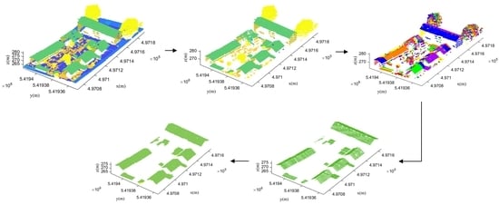
Graphical Abstract

1. Introduction

A building is an essential component of urban construction. The extraction and reconstruction of buildings has been a critical step for many applications, such as urban planning, disaster assessment, cadastral management and so on [1,2]. Airborne LiDAR is an active remote sensing technology which has developed very rapidly in the recent years [3,4,5,6]. This technology has become an attractive choice for building extraction [7,8], due to its high efficiency and measuring accuracy, less interference by external environment and strong initiative [9,10].

1.1. Related Works

Currently, building extraction methods can be classified into two categories, including the machine learning methods and the classic methods. In the machine learning methods, the acquired raw data are first transformed into a multidimensional feature space. Then, an optimal feature space is estimated by a learning classifier to map the features into desired outputs [11]. Ni et al. [12] first proposed a stepwise point cloud segmentation method to extract three kinds of segments, including planar, smooth and rough surfaces. Random Forest (RF) was then employed to select features and classify the afore-mentioned segments. Finally, semantic rules were used to optimize the classification result. The experimental results showed that this method was effective for small scale targets. Nahhas et al. [13] proposed a deep learning method to detect buildings by fusing the LiDAR data and orthophotos. In this method, features were first extracted by object-based analysis. The low-level features were transformed into compressed features with a feature-level fusion and an autoencoder-based dimensionality. After that, the compressed features were transformed into the high-level features using a Convolutional Neural Network (CNN) to classify the objects into buildings and background. Maltezos et al. [11] also adopted a CNN model in their method. Firstly, a multi-dimensional feature vector was created using the raw LiDAR data and seven additional features. Experimental results showed that this algorithm could extract buildings with 85% completeness, and the correctness reached 93%, at per-area level. Huang et al. [14] fused high-resolution aerial images and LiDAR points for building extraction with an end-to-end trainable gated residual refinement network. The modified residual learning network was applied as the encoder part of network to learn multi-level features from the fusion data. A gated feature labeling unit was introduced to reduce unnecessary feature transmission and refine classification results. Zhang et al. [7] developed a hybrid attention-aware fusion network based on a novel hybrid fusion architecture to extract the buildings from high-resolution imagery and LiDAR data. Li et al. [15] first split the raw preprocessed LiDAR data into numerous samples to fed into CNNs directly. Then, the graph geometric moments CNNs were proposed to train and recognize building points. Finally, the test scenes were fed into the framework to extract the building points. Wen et al. [6] first proposed a graph attention convolution module. This module could examine spatial relationship among all points and determine the convolution weights. Then, a global-local graph attention CNN was designed to classify the airborne point clouds using multiscale features of the point clouds. Yuan et al. [16] proposed a fully CNN based on the residual network. The training pattern for multi-modal data was provided by combining the advantage of high-resolution aerial images and LiDAR data. Obviously, for the CNN models, the precise labelled point clouds are generally necessary. Zolanvari et al. [17] provided a publicly available annotated benchmark dataset for training and testing. Moreover, they also tested three well-known CNN models, including PointNet, PointNet++ and So-Net on the benchmark. In addition to the geometric features built for the machine learning techniques, some researchers try to calculate the statistical characteristics of the point cloud distribution to realize unsupervised segmentation [18]. For instance, Crosilla et al. [19] proposed a filtering and classification technique for LiDAR points by calculating the statistical features, including skewness and kurtosis iteratively. Specifically, the skewness and kurtosis are third- and fourth-order moments about the mean.
Although the machine learning methods can realize building extraction, these methods unavoidably involve some limitations. For instance, high-quality training data are required, and the differences in the data distribution between the training data and the experiment scenes lead to low accuracy [20]. To avoid these problems, some authors work on the classic methods. In terms of input data, methods can be further classified as two categories, including building extraction based on LiDAR points and based on multi-source data fusion [15]. In the first type of methods, LiDAR points are the only data source for building extraction. In these methods, building points are extracted by relying mainly on their geometric morphological features that are different from other objects. Dorninger et al. [21] proposed a building extraction method based on plane segmentation detection. The hierarchical clustering algorithm was used to obtain the initial candidate seed points. Then, they extracted the buildings with the iterative region growing algorithm. Poullis et al. [22] used the object-based region growing algorithm to detect the building points and refined the boundary with a polygon Boolean operation to achieve better building extraction results. In Sun et al. [23], point cloud data were divided into ground and non-ground points with a graph cut-based method where a novel hierarchical Euclidean clustering method was used to extract rooftop patches. Finally, a region growing-based segmentation method was presented to detect all building points with each rooftop patch. Awrangjeb and Fraser [24] separated the raw LiDAR points into two groups and formed a “building mask” with the group containing the ground points. The group that contains non-ground points was segmented into individual building or tree objects using the building mask. During the segmentation, the planar roof segments were extracted and refined based on the rules, such as the coplanarity, locality and height difference of points. The experimental results showed that this method offered a high successful rate for building detection and roof plane extraction. Fan et al. [25] realized the building extraction based on the fact that each roof can be composed of gabled roofs and single flats. The algorithm Random Sample Consensus (RANSAC) was then used to detect roof ridges. Then, the points on the two roof flats along a roof ridge were identified based on their connectivity and coplanarity. Sampath et al. [26] first analyzed point characteristics to exclude the nonplanar points. The authors used the fuzzy k-means algorithm to cluster the planar points. To extract complete buildings, the clustered points were merged into the integrated rooftop according to the breaklines. Zou et al. [27] proposed a strip strategy-based method to filter the building points and extract the edge point set from LiDAR data. The point cloud was segmented into several data strips. After that, building points were filtered from the data strips with an adaptive-weight polynomial. Finally, building edges were extracted by a modified scanline method. This method is usually suitable for urban areas where buildings were densely distributed. Cai et al. [28] introduced a coarse-to-fine building detection method that was based on semi-suppressed fuzzy C-means and restricted region growing. After a minimum bounding rectangle was adopted to refine the detection results, the method could offer an excellent performance for building detection with over 89.5% completeness and a minimum 91% correctness. In Wang et al. [29], a semantic-based method was employed to extract building points with contexts. A Markov random field optimization model was constructed for postprocessing and segmentation results refinement.
Although the building extraction methods using only LiDAR data can achieve good extraction results, these methods unavoidably have some practical limitations. For instance, the laser pulses emitted by airborne LiDAR system often have a certain tilt angle, resulting in the absence of points in some areas [30]. These data gaps will result in incomplete building extraction. Although LiDAR data provide accurate three-dimensional coordinates, they lack texture information that is very important for identifying buildings with special shapes [31]. To overcome these enumerated limitations, some authors integrate multi-source data to achieve high accuracy. Authors such as Awrangjeb et al. [32] proposed an automatic three-dimensional roof extraction method by combining LiDAR data and multi-spectral orthoimages. In their study, the Normalized Difference Vegetation Index (NDVI) from multi-spectral orthoimages and the entropy images from grayscale orthoimage were first used to generate a Digital Elevation Model (DEM). Afterwards, the DEM was used to separate ground and non-ground points, while the NDVI and entropy images were used to classify the structure lines extracted from grayscale images. Structural lines belonging to the building class were then used to extract the plane and edge of the roof. Finally, the roof planes and boundaries were extracted using the lines belonging to the building class. They further added texture information from the orthoimage and used an iterative region growing algorithm to extract the complete roof plane, which improved the completeness of building extraction [33]. Qin et al. [34] combined the high-resolution remotely sensed image and Digital Surface Model (DSM). The morphological index was first used to detect shadows and correct the NDVI. Then, the NDVI was incorporated through the reconstruction of the DEM using the top-hat algorithm to obtain the initial building mask. Finally, the building segments with high probability were consolidated by a graph cut optimization based on modified superpixel segmentation. The experimental results showed that this algorithm could extract buildings efficiently with 94% completeness, and the 87% correctness indicating its potential for many practical applications. Gilani et al. [35] developed a methodology using features from point cloud and orthoimage to extract and regularize the buildings. Vegetation elimination, building detection and extraction of their partially occluded parts were achieved by synthesizing the entropy, NDVI and elevation difference. Results indicated that the per-area completeness achieved was between 83% to 93%, while the per-area correctness was above 95%. Siddiqui et al. [36] transformed the LiDAR height information into intensity and then analyzed the gradient information in the image. In addition, a local color matching approach was introduced as a post-processing step to eliminate trees. Lai et al. [37] proposed a building extraction method by fusing the point cloud and texture features. The texture features were acquired using an elevation map. Chen et al. [38] also integrated high spatial resolution images and LiDAR point cloud data. In their method, an adaptive iterative segmentation method was adopted to effectively avoid over-segmentation or under-segmentation.

1.2. Motivation

Although more accurate building extraction results can be achieved by fusing multi-source remote sensing data, pre-registration is generally required [39]. Registration errors often exist during the fusion process, and how to provide registration accuracy remains an unsolved problem [40]. Therefore, building extraction with only LiDAR points is still a mainstream focus. Today, although the machine learning methods have been successfully applied for building extraction, large numbers of sample labeling are generally a prerequisite for the success of this kind of methods. Obviously, the sample labeling is always cumbersome. Thus, how to realize building extraction by classic methods is still in the focus of researchers. However, the classic building extraction methods based solely on airborne LiDAR points still involve the following difficulties and challenges:
  • The point-based building extraction methods generally involve high computation costs. Thus, it is difficult to process a large amount of LiDAR points.
  • When encountering with different building environments, the performance of the methods generally varies greatly. The robustness of the building extraction methods is not good.
  • The vegetation points adjacent to buildings are easily misclassified as building points, which results in low correctness of building extraction.
To solve these enumerated problems, a building extraction method from airborne LiDAR points based on multi-constraints graph segmentation was proposed in this paper. In the proposed method, the graph structure was first constructed based on the three-dimensional spatial features of points. Then, the graph segmentation was achieved by setting constraint conditions. In doing so, the point-based building extraction was transformed into the object-based building extraction to reduce the computation cost and improve the efficiency of the method. Subsequently, the initial building points were extracted by calculating the geometric morphological features of each segmented object. To improve the completeness of building extraction, this paper also proposed a multi-scale progressive growing optimization method to recover the omitted building points. Three publicly available datasets were adopted for testing the performance of the proposed method. The experimental results showed that the proposed method can achieve very good building extraction results.

2. Methodology

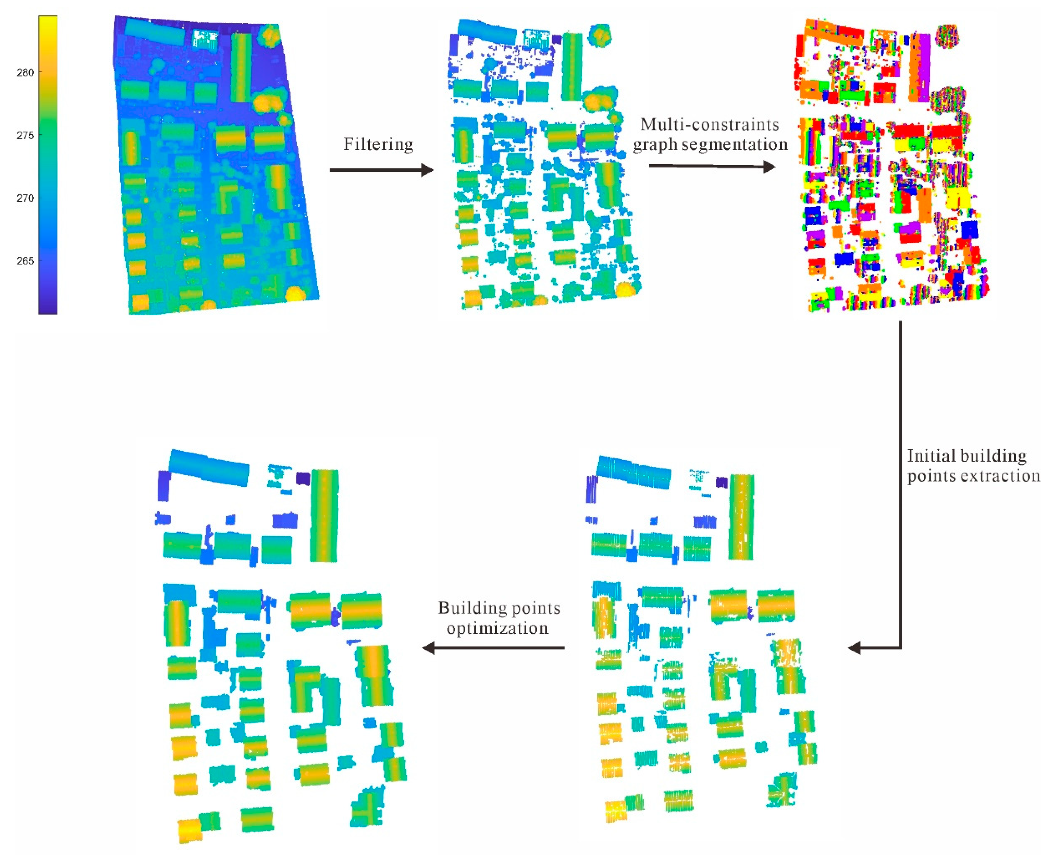
The flowchart of the proposed method is shown in Figure 1. In this paper, an improved morphological filtering method based on kriging interpolation proposed by Hui et al. [41] was first adopted to remove ground points. This filtering method can be seen as a hybrid model, which combined the morphology-based and the interpolation-based filtering methods. By removing objects and generating rough ground surface progressively, the terrain details can be protected successfully. Subsequently, the multi-constraints graph segmentation method was proposed to segment the non-ground points to obtain the object primitives. Hereafter, the point-based building extraction was transformed into the object-based building extraction, which reduced the computational cost and improved the implementation efficiency of the proposed method. Here, the initial building points are acquired by calculating the spatial geometric features of each object primitive. To improve the completeness of building extraction, this paper proposed a multi-scale progressive growth optimization method. This method was used to extract complete buildings by continuously recovering the omitted points that meet the setting rules. Detailed description of the proposed method is described in the subsequent sections as follows: Section 2.1, multi-constraints graph segmentation; Section 2.2, initial building points extraction based on spatial geometric features; and Section 2.3, building points optimization based on multi-scale progressive growing.

2.1. Multi-Constraints Graph Segmentation

To reduce the computation costs and improve the efficiency of the proposed method, this paper first transforms the point-based building extraction method into an object-based building extraction method. In this paper, the transformation is realized based on multi-constraints graph segmentation. Generally, the graph structure can be defined as Equation (1) [42]:
G = ( V , E )
where G represents the graph, V is the set of nodes ( v i ) and E denotes the corresponding edges ( e i , j ). In this paper, v i is made up of all points ( p i , i = 1 , 2 , , N ) in the point cloud, while the edge e i , j connects the pair of neighboring points ( p i , p j ).
Today, with the fast development of the LiDAR system, the density of the LiDAR points can reach hundreds of points per square meter. For instance, the average point density of the acquired aerial LiDAR datasets of Dublin city center is 348.43 points/m2 [17]. As a result, a huge amount of LiDAR data generally needs to be processed. If the graph is constructed using edges between every point, the built graph will be very complex and cost lots of computer memory. Moreover, it will also not be conducive to subsequent graph segmentation. To simplify the graph, this paper proposed several constraints for building the graph. The first constraint is that the edge e i , j only exists among neighboring points. This can be defined as Equation (2):
e i , j = { 1 , i f p j S e t p i 0 , o t h e r w i s e
where S e t p i is k nearest neighbors of point p i . In Equation (2), it can be deduced that only if p j is an adjacent point to p i , there will be an edge connection between two points. k is a constant which represents the number of neighboring points. If the number of points is massive or the calculating capability of computer hardware is limited, k should not be set too large. Otherwise, the computation costs will increase. In this paper, k is set to 10.
Aiming at achieving the accurate building object primitives, two other constraints were set after the graph construction. On the one hand, the points within an identical object primitive should own similar normal vectors. That is, the edge between p i and p j can be reserved only if the angle between the normal vectors of the two points is less than a threshold. This can be defined as Equation (3):
e i , j = { 1 , i f θ ( p i , p j ) ς 0 , o t h e r w i s e
where θ ( p i , p j ) is the angle between the normal vectors of p i and p j . The normal vector of a point can be estimated from the covariance matrix of its neighboring points using Principal Component Analysis (PCA). The eigenvector corresponding to the minimum eigenvalue of the covariance matrix is treated as the normal vector at the point. ς is the angle threshold. In this paper, ς is set to 5° to maintain the similarity of points within the same object primitives.
When the normal vector constraint is applied, the points located on the same plane will be divided into the same object primitives, such as the building roofs, as shown in Figure 2a. Conversely, some adjacent points that are not in the same plane will be divided into multiple object primitives, such as vegetation. However, if only the normal vector constraint is adopted, some vegetation points that are adjacent to buildings will be misclassified as building points, as shown in Figure 2b,c. It is because the normal vectors of these vegetation points may be similar to the ones of the building points, which may lead to misjudgment. To solve this problem, the third constraint of graph segmentation that is the longest edge constraint is defined as Equation (4):
e i , j = { 1 , i f D i s t ( p i , p j ) m e a n ( D i s t ( S e t p i ) ) + s t d ( D i s t ( S e t p i ) ) 0 , o t h e r w i s e
where D i s t ( p i , p j ) is the Euclidean distance between p i and p j . m e a n ( D i s t ( S e t p i ) ) represents the mean distance from point p i to all its neighbors. s t d ( D i s t ( S e t p i ) ) is the standard deviation of the distance from point p i to all its neighbors. This constraint will limit the range of the longest edge and avoids the problem that some adjacent vegetation points can be misclassified as building points.

2.2. Initial Building Points Extraction Based on Spatial Geometric Features

As shown in Figure 2a, the point cloud is divided into multiple object primitives after the multi-constraints graph segmentation. Since the angle of normal vectors and the longest edge constraints were adopted in the multi-constraints graph segmentation, the building roofs can be correctly divided into independent object primitives, as shown in Figure 2b,c. However, some other objects without similar normal vectors, such as bushes, vegetation and fences, are generally divided into multiple small object primitives, which will lead to “over-segmentation”. According to this characteristic, the initial building points can be extracted based on the spatial geometric features of the extracted object primitives. In this paper, the roughness and size of object primitives were selected to extract the initial building point cloud.
In this paper, the object primitive roughness ( r o u g h n e s s o b j i ) is defined as the mean distance residual between the point and the best-fit plane of the points within the same object primitive. This has been defined in Equation (5) as:
{ r o u g h n e s s o b j i = i = 1 n r o u g h n e s s p i n r o u g h n e s s p i = | A x p i + B y p i + C z p i + D | A 2 + B 2 + C 2
where r o u g h n e s s p i is the roughness of p i in an object primitive o b j i . r o u g h n e s s p i is defined as the distance residual between the point to the fitting plane ( A x + B y + C z + D = 0 ).
Generally speaking, for a relatively flat roof, the object primitive roughness of a building tends to be smaller than that of the pseudo plane generated by dense vegetation points. Compared with the over-segmented object primitives, building object primitives often contain more points. Meanwhile, the non-building object primitives are generally divided into several small object primitives since the direction of their normal vectors are not consistent. Therefore, the non-building object primitives can be removed by limiting the size of object primitives to further improve the accuracy of the initial building points extraction.

2.3. Building Points Optimization Based on Multi-Scale Progressive Growing

Although most of the building points can be correctly extracted based on the spatial geometric features of the object primitives, there are still some omitted building points, which will cause larger omission error. As shown in Figure 3, the omitted building points are mainly located on the ridge and edge area of the roof. These points are easily divided into different object primitives after multi-constraints graph segmentation since their spatial geometric features are generally quite different from their adjacent points. As a result, these ridge or edge points are wrongly eliminated, which can result in low completeness of building extraction.
To improve the completeness of the building points extraction, this paper proposed a building points optimization method based on multi-scale progressive growing. The pseudocode of the proposed method is presented in Algorithm 1.
Algorithm 1. Building points optimization based on multi-scale progressive growing.
Input:Initial building points: P o int _ s e t = { p i | p i U p i U } , i = 1 , 2 , , N
p i is a random point, U is the building point set, U is the complementary set, which represents a non-building point set.
Scale sets: s = { s 1 , s 2 , , s K } , s 1 > s 2 > > s K
for iter = 1 to K
s = siter
  for i = 1 to N
   if p i U
      Find the neighboring point set of p i under the scale of s: S e t p i = { p j | D i s t p j , p i s , j = 1 , 2 , , M }
     for j = 1 to M
      if p j S e t p i & & p j U
       Calculate the distance ( d i s t p j ) between p j and the fitting plane of the object primitives where p i is
       Calculate the angle ( θ ( p j , p i ) ) between the normal vector of p j and p i
        if d i s t p j t h 1   | |   θ ( p j , p i ) ξ
         p j U
   Update building point set U and non-building point set U
end
Output: Building points set U
From Algorithm 1, it can be found that this paper mainly adopted a multi-scale progressive strategy to gradually optimize the building points extraction results. Through experimental analysis, three fixed scales are enough to acquire complete building points. In doing so, not only the problem of overgrowth can be solved but also the implementation efficiency can be improved. In this paper, the scale sets are defined as s 1 (2 m), s 2 (1.5 m) and s 3 (0.5 m), respectively. In each step, the neighboring points set of each point is obtained within the current scale. If p j is a non-building point in the neighboring points set ( S e t p i ) of p i , the distance residual ( d i s t p j ) between p j and the fitting plane of the object primitive should be calculated. If p j is an omitted building point, the distance residual will be less than the threshold t h 1 , which is set to 0.3 m in this paper. In addition, building point clouds often have consistent normal vectors. Thus, if p j is an omitted building point, the angle between the normal vectors of p j and p i should be less than the angle threshold ξ which is set to 10° in this paper.

3. Experimental Results and Analysis

3.1. Experimental Datasets

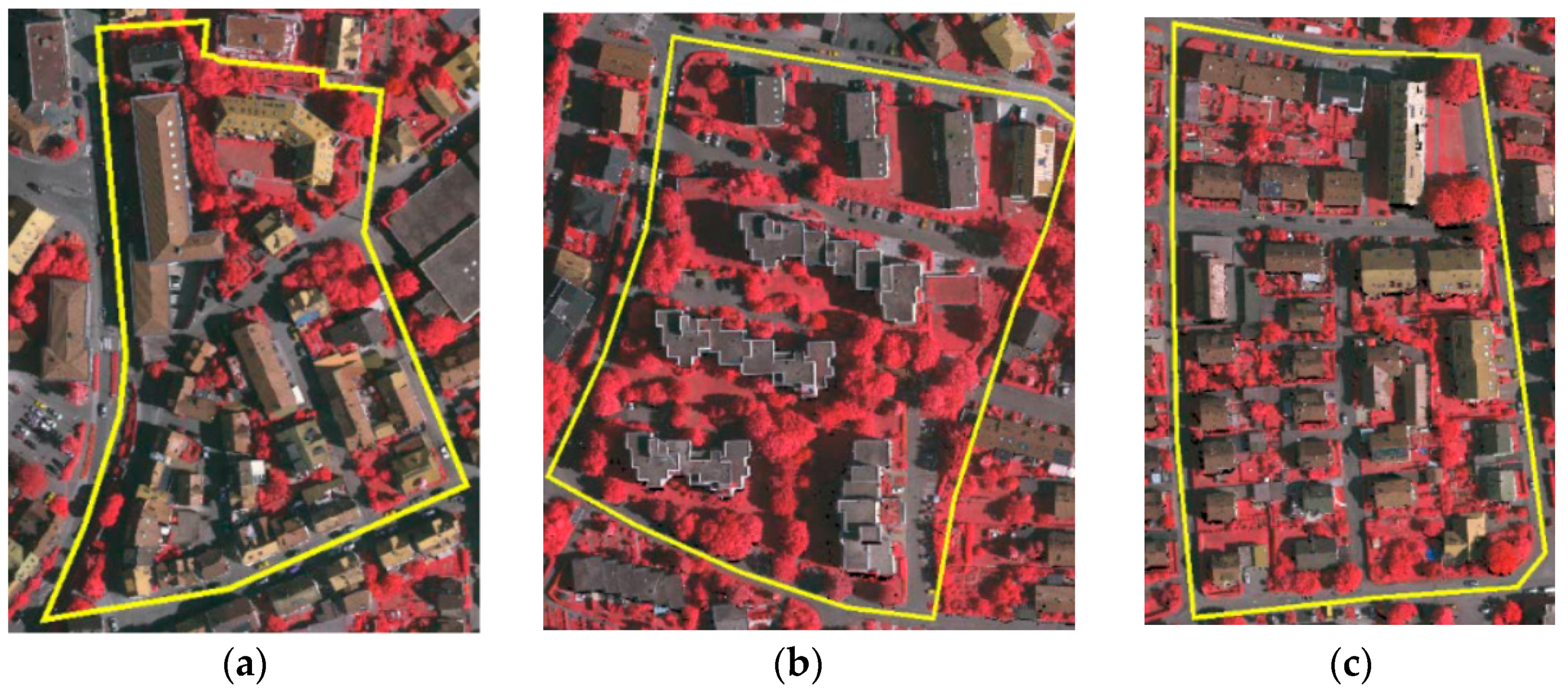
To evaluate the performance of the proposed method, three publicly available datasets provided by ISPRS were tested [43]. The datasets were obtained by Leica ALS50 with a 45° field of view and a 500 m mean flight height above the ground. The obtained points’ accuracy is approximately 0.1 m in horizontal and vertical directions. The average strip overlap is 30%, and the average point density is 4–7 points/m2. The three datasets are located in Vaihingen and contain three areas (Area1, Area2, Area3). As shown in Figure 4, the main objects in the three areas are powerline, low vegetation, impervious surfaces, car, building, shrub, tree and fence and so on. The buildings in Area1 are with complex shapes and different sizes as shown in Figure 4a. Thus, Area1 can be used to test the extraction accuracy of the proposed method on complex buildings. Area2 is characterized by buildings surrounding with dense vegetation (Figure 4b). Adjacent vegetation often causes great interference on the building extraction. Therefore, Area2 can verify whether the proposed method effectively eliminates the interference of adjacent vegetation or not. In Area3, as shown in Figure 4c, low vegetation is the main challenge to the building extraction. How to eliminate the pseudo planes formed by the low vegetation is still an unresolved problem. Thus, it can be concluded that the three datasets are a good representation for testing the effectiveness and robustness of the proposed method for building extraction in different environments.

3.2. Experimental Results and Analysis

Figure 5 shows the building extraction results using the proposed method. From Figure 5, most of the buildings can be extracted correctly so as to achieve good building extraction accuracy in the three experimental areas. As shown in Figure 5a,d, although there are many buildings with complex shapes and different sizes in Area1, the proposed method can extract them correctly. Thus, it can be concluded that the proposed method is robust towards building with different shapes and sizes. However, there are still some omitted building points in Area1 (the blue points in Figure 5a,d), which are mainly located at the edge of the building. It is because these buildings are generally with low elevation. Due to the height difference, the low buildings cannot form a complete object primitive along with the adjacent buildings but form an independent object primitive. Since the size constraint of object primitives is adopted in the initial building extraction step, these small object primitives will be wrongly removed. Although there is dense adjacent vegetation in Area2, the proposed method effectively eliminates its interference on building extraction. However, there are still some points that are wrongly classified as buildings, as shown by the red points in Figure 5b,e. It is because the buildings in Area2 are stacked and the facades of some buildings are connected with the roofs. As a result, they are easily misclassified as roof points. The building extraction accuracy of the proposed method in Area3 is relatively high due to the simple features of the buildings in it. Some omitted points are located near the chimneys because of the spatial differences among the chimneys with the roof (Figure 5c,f).
For quantitative evaluation, four indicators proposed by Rutzinger et al. [44] were adopted to evaluate the precision of the building detection results at both pixel-based and object-based levels. They are completeness ( C o m p ), correctness ( C o r r ), quality ( Q u a l i t y ) and F1 score ( F 1 ).
Completeness represents the percentage of buildings in the reference that were detected. Correctness indicates how well the detected buildings match the reference. Completeness tends to evaluate the ability of building detection, while correctness evaluates the correct detection ability of the proposed method. Quality and F1 score are another two indicators, which can integrate completeness and correctness to reflect the effectiveness of the method. The definitions of the above four indicators are defined in Equations (6)–(9):
C o m p = T P T P + F N
C o r r = T P T P + F P
Q u a l i t y = C o m p × C o r r C o m p + C o r r C o m p × C o r r
F 1 = 2 × C o m p × C o r r C o m p + C o r r
This paper evaluated the performance of the proposed method at pixel-based and object-based levels, respectively. In the pixel-based evaluation, T P represents the number of correctly extracted building points, F N is the number of omitted building points, FP represents the number of wrongly detected building points. In the object-based evaluation, the object can be accepted as T P if it has a 50% minimum overlap with the reference data. F N represents the number of omitted building objects, F P is the number of objects whose overlap ratio is less than 50% with the reference data [45].
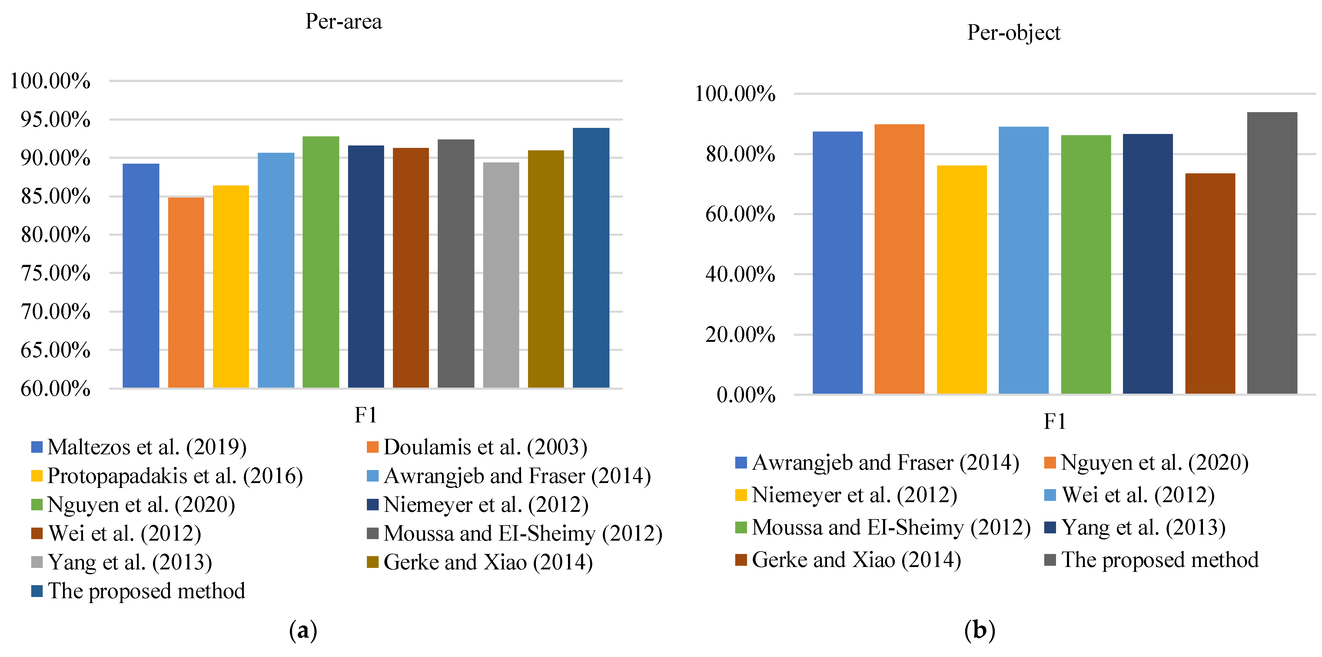
To evaluate the performance of the proposed method objectively, this paper selected other ten methods that have also used these public datasets provided by ISPRS for comparative analysis. Among the ten methods, the first three methods belong to the kind of machine learning method, while the other seven methods belong to the kind of classic methods. Maltezos et al. [11] first created a multi-dimensional feature vector using the raw LiDAR data and the seven additional features. Then, a CNN was used to nonlinearly transform the input data into abstract forms of representations. After that, a training set was used to learn the parameters of the CNN model to perform the building extraction. Doulamis et al. [46] developed a radial base function kernel Support Vector Machine (SVM) classifier. The classifier adopted an efficient recursive weight estimation algorithm to make the network response adaptive. Protopapadakis et al. [47] proposed a nonlinear scheme of a typical feed-forward artificial neural network with a hidden layer. When the appropriate features were fed to the detection model, the optimal parameters of the detector structure were selected by an island genetic algorithm. Awrangjeb and Fraser [24] formed a “building mask” using the ground points, and then extracted building and vegetation objects with the co-planarity between adjacent points. After that, vegetation plane primitives were removed by using the information of area and neighborhood characteristics to complete the building extraction. Nguyen et al. [45] presented an unsupervised classification method called super-resolution-based snake model to extract buildings by combining the spectral features of images and LiDAR point cloud. Niemeyer et al. [48] established the classification model with a conditional random field approach. This method utilized a nonlinear decision surface to separate the object clusters in feature space reliably, and then extracted buildings. Wei et al. [49] presented an integrated method to comprehensively evaluate the feature relevance of point cloud and image data. Firstly, point cloud and image data were co-registered. After that, all data points were grid-fitted to facilitate acquiring spatial context information per pixel/point. Then, spatial-statistical and radiometric features could be extracted using a cylindrical volume neighborhood of point. Finally, the AdaBoost classifier combined with contribution ratio was used to label the points. Moussa and EI-Sheimy [50] fused the aerial images data with single return LiDAR data to extract buildings for an urban area. Then, they segmented the entire DSM data into objects based on height variation. After that, the area, average height, and vegetation index of each object were adopted to exactly classify the objects. Yang et al. [51] defined the Gibbs energy model of building objects within the framework of reversible-jump Markov Chain Monte Carlo to describe the building points. Then, they found an optimal energy configuration using simulated annealing. Finally, the detected building objects were refined to eliminate false detection. Gerke and Xiao [52] introduced a new segmentation approach by making use of geometric and spectral data. They quantified the point cloud into voxels according to the geometric and textural features of optical images, and then, buildings are extracted from voxels by using the supervised classification method based on random forest. Note that the methods proposed by Maltezos et al. [11], Doulamis et al. [46] and Protopapadakis et al. [47] only provide the completeness, correctness and quality at per-area level. The F1 score can be calculated according to Equation (9). Thus, in Table 1, Table 2 and Table 3, we only compared their building performance at per-area level. It is the same with Figure 6 and Figure 7, only the average quality and F1 score of the three methods at per-area level were compared with other methods.
Table 1, Table 2 and Table 3 show the accuracy comparison of the proposed method with the ten methods described above in the three areas (Area1, Area2 and Area3) at per-area and per-object levels. From the comparison, it can be found that the satisfying results in the three areas are obtained by the proposed method. All the four indicators (completeness, correctness, quality and F1 score) of the proposed method of the three testing areas are higher than 85%, and most of them are higher than 90%. The results indicate that the proposed method can obtain highly desirable accuracy in different environments and can robustly extract buildings. In the three areas, the proposed method achieved the best on six out of eight indicators with four indicators at per-area and per-object levels, respectively. Therefore, compared with the other investigated methods, the proposed method has the best building extraction performance. In Area1, the proposed method achieved the highest completeness (Table 1) at both per-area and per-object levels, which demonstrates that the proposed method has a strong capability of building detection. Compared with the other two areas, the proposed method performed best in Area2, and all indicators were higher than 90%, as shown in Table 2. Especially in the per-object evaluation, the quality of the proposed method (90.32%) is significantly better than the other methods. This indicates that the proposed method can effectively overcome the interference caused by dense vegetation around buildings, and can achieve the correct extraction of buildings. In Area3, the per-area correctness of the proposed method can reach 97.59% (Table 3). It shows that the proposed method can detect buildings correctly. Overall, the completeness and correctness of the proposed method are relatively balanced, which indicates that the proposed method can extract as many buildings as possible while ensuring the correctness of the extraction results.
Figure 6 and Figure 7 show the comparison of average quality and average F1 score of the proposed method with the other ten methods in the three study areas. In terms of the average quality, the proposed method achieved the best results in both per-area and per-object evaluations. Especially, at per-object level, the average quality of the proposed method is obviously better than that of the other seven methods. In addition, the proposed method also obtained the highest average F1 score. Both at per-area and per-object levels, the average F1 score of the proposed method is more than 90%. Consequently, the proposed method performed well in the three kinds of building environments and thus can be considered as relatively robust.

4. Discussion

In the multi-constraints graph segmentation, two parameters are involved, namely the number of neighboring points k and the angle threshold ς . The number of neighboring points determines the size of neighboring set (Equation (1)), while the angle threshold (Equation (2)) directly affects segmentation results. These two parameters determine the selection of edges directly and have a distinct influence on the results of graph construction. Concretely, the larger the k value, the more edges will be accepted, thereby complicating the graph, increasing the computational costs, and reducing the efficiency of the method. In the last two decades, some techniques have been proposed to determine the k neighbors, such as the lowest entropy or highest similarity [53]. In terms of the lowest entropy, the Shannon entropy has to be calculated for every point. The optimal radius can be determined by calculating the lowest entropy. In terms of the highest similarity, a similarity index is defined as the ratio of neighbors whose dimensionality labelling is same with that of the center point. The optimal radius can be obtained by finding the highest similarity index for each point. Although these optimal radius selection techniques can help to determine the k neighbors, it will involve too much calculation. Obviously, the computational burden will increase greatly and the optimal radius selection process will be time consuming. To facilitate the implementation of the proposed method, this paper set a fixed value for the neighbors. Through experimental analysis, the graph complexity and the efficiency can be balanced when the value of k is set to 10.
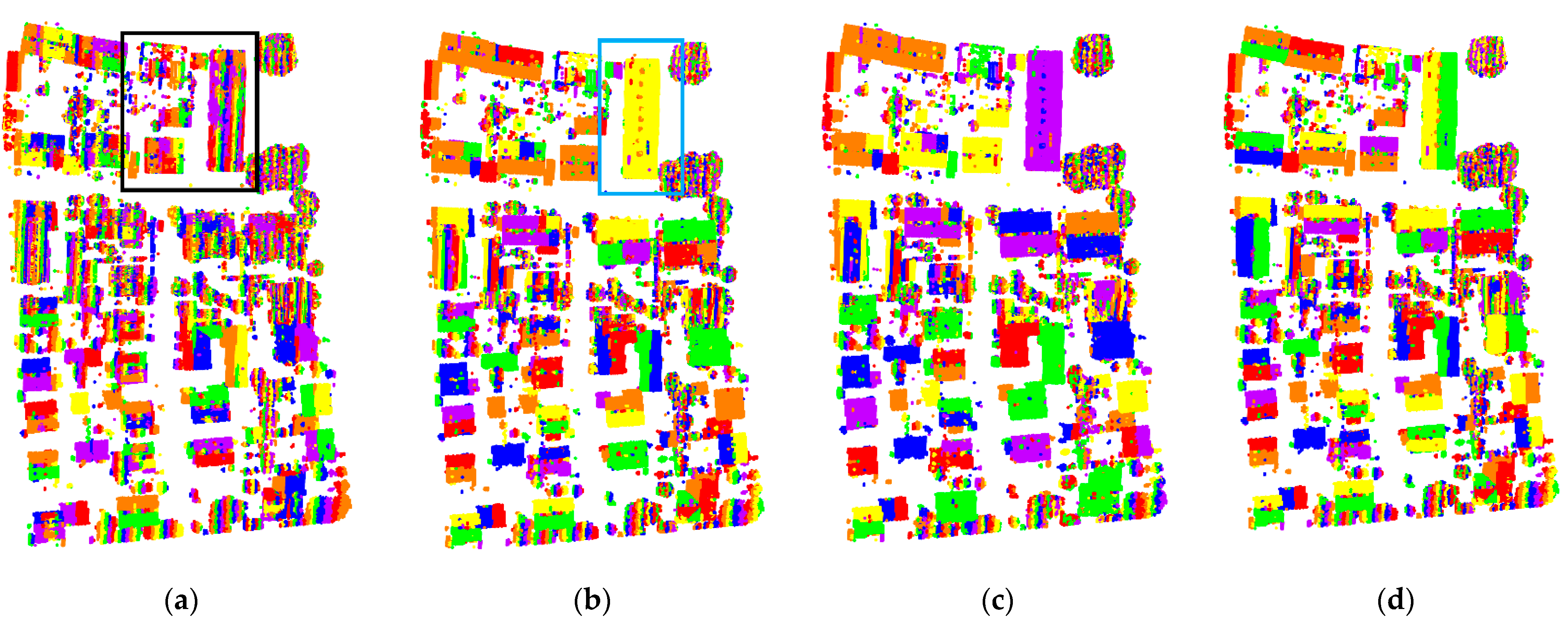
The angle threshold ς was set to divide the points on the same plane into the same object primitives, while the points on different planes were split into multiple object primitives. Figure 8a–c shows the results of multi-constraints graph segmentation results with ς taken as 1°, 10° and 15°, respectively. Figure 8d shows the reference segmentation results. Although vegetation points were divided into multiple object primitives, the same building roof was also separated into several small object primitives when ς was set to 1°, as the black rectangle shown in Figure 8a. This over-segmentation phenomenon is not conducive to the subsequent extraction of initial building points which are based on the size of object primitives. When ς was set to 10°, some points on different roof planes of the building failed to be separated into different object primitives, as shown in Figure 8b as blue rectangle. When the value of ς continues to increase ( ς = 15°), a more under-segmented roof planes were observed, as shown in Figure 8c. If the points from different roof planes are segmented into same object primitives, there will be a large fitting error in calculating the roughness of each object primitive. Consequently, it will be difficult to discriminate buildings from other object primitives (such as dense vegetation). The experimental results showed that the proper segmentation results can be achieved when the angle threshold ς is set to 5°, as shown in Figure 2a. In this case, not only the vegetation points can be divided into multiple object primitives, but also the building points from the same plane can be separated into the same object primitives.
Another important parameter involved in this paper is the threshold for the object primitive roughness, which was set in the step of initial building extraction. Figure 9a–c are the initial building extraction results for Area3 with the roughness thresholds of 0.02, 0.04 and 0.06, respectively. In Figure 9a, it can be found that when the value of this threshold was too small, many independent buildings were not successfully detected. It is because that part of the points located at the boundary of buildings were omitted, resulting in the low completeness of the initial building points. Figure 9b shows the initial buildings extracted in this paper with the roughness threshold of 0.04. It illustrates that, with the proper value of the threshold, more buildings could be detected, and the misclassification of some non-building points can be avoided. When the threshold is set too large, it can be found that mainly dense vegetation points are misclassified as buildings, as shown in Figure 9c. Therefore, setting a too large roughness threshold will reduce the correctness of the result.
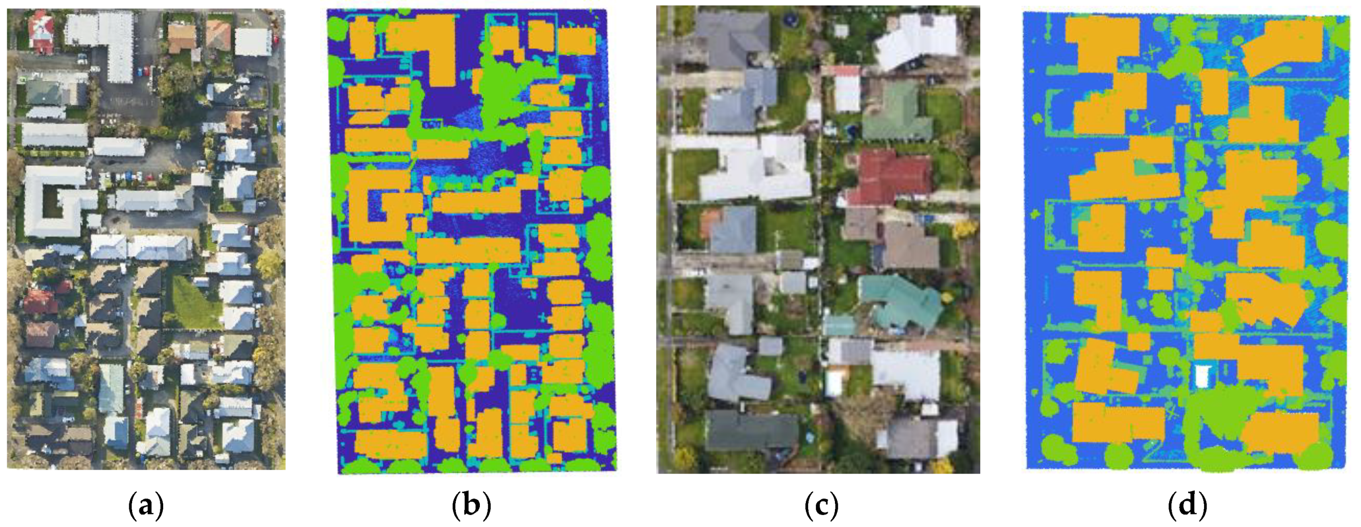
To validate the applicability of the proposed method, two other public datasets provided by OpenTopography were selected for further testing [54]. The datasets are located in the north of Palmerston, New Zealand, with a point density of 22 points/m2. The ground objects include buildings, impervious surface, low vegetation, trees and shrubs and so on, as shown in Figure 10. Figure 10a is the true-color image of the first dataset named as S1. It can be seen that the buildings in S1 are densely distributed with regular shapes, surrounded by dense vegetation. Figure 10b is the point cloud data of this area. Figure 10c is the true-color image of the second dataset named as S2, which contains many buildings with complex shapes and large sizes. Figure 10d shows the corresponding point cloud data of this area.
The building extraction results of the two areas mentioned above are shown in Figure 11. Figure 11b,d are the reference building extraction results from the orthophoto images of S1 and S2, respectively. It can be found that the proposed method can achieve satisfying results in both areas (S1 and S2) because most of the building points were accurately extracted. However, there still exist some points on the roof plane that were not effectively detected as shown as blue points in the black rectangle of Figure 11a. It is mainly because there are some small roof planes in S1, which makes the object primitives formed by these blue points smaller so that they cannot be effectively identified in the initial building extraction. As shown in Figure 11c, there are a few wrongly detected points in S2, such as the red points in the black rectangle. It is caused by the overlapping of some high vegetation and buildings. A small number of vegetation points around the edge of buildings are divided into the same object primitives with their adjacent buildings, thereby being misclassified. Table 4 shows the quantitative evaluation results of the two areas. All the indicators are higher than 90%. Especially, the completeness and F1 score of the proposed method are higher than 95%. Thus, it can be concluded that the proposed method can effectively detect buildings with different sizes and shapes.

5. Conclusions

Building extraction from airborne LiDAR point clouds is a significant step in the applications of point cloud post-processing, such as urban three-dimensional model construction and digital urban management. To solve the problems existing in the building extraction, such as huge computational cost, poor adaptability to different building environments and the interference of adjacent vegetation, this paper proposed a building extraction method from airborne LiDAR data based on multi-constraints graph segmentation. In this paper, the graph structure of the point cloud was first built. Afterwards, the object primitives were obtained based on the multi-constraints graph segmentation. In doing so, the point-based building extraction is transformed into the object-based building extraction to improve the efficiency of the method. After that, the initial building point cloud is extracted based on the different spatial geometric features of each object primitive. To improve the completeness of building extraction, this paper proposed a multi-scale progressive growth optimization method to recover some omitted building points located on the ridge and edge areas. Three public datasets with different building environments provided by ISPRS were adopted for the testing. The experimental results showed that the proposed method can achieve good building extraction performance in all the three testing areas. Compared with other ten famous building extraction methods, the proposed method also performed the best. Two other publicly available datasets provided by the OpenTopography were also used for further testing. The experimental results showed that the proposed method has strong robustness and promising performance in building extraction. In addition, the completeness and correctness achieved by this method were relatively high and balanced. It reveals that the proposed method can detect more buildings while ensuring the accuracy of the results. However, the implementation of the proposed method needs setting of some parameters, such as the number of neighboring points k and the angle threshold ς . To ease the implementation of the proposed method, this paper set fixed values for the parameters. However, to obtain better building extraction results, it is necessary to adjust the parameters according to the point clouds with different densities. In future work, we will try to improve the automation of the proposed method to make the parameters adjusting automatically according to the particularity of each point cloud.

Author Contributions

Z.H. conceived the original idea of the study and drafted the manuscript. Z.L. and P.C. performed the experiments and made the experimental analysis. Y.Y.Z. and J.F. contributed to the revision of the manuscript. All authors have read and agreed to the published version of the manuscript.

Funding

This work was supported by the China Post-Doctoral Science Foundation (2019M661858), the National Natural Science Foundation of China (NSF) (41801325, 42161060, 41861052), the Natural Science Foundation of Jiangxi Province (20192BAB217010), Education Department of Jiangxi Province (GJJ170449), Key Laboratory for Digital Land and Resources of Jiangxi Province, East China University of Technology (DLLJ201806), East China University of Technology Ph.D. Project (DHBK2017155) for their financial support.

Institutional Review Board Statement

Not applicable.

Informed Consent Statement

Not applicable.

Data Availability Statement

The first three publicly available datasets were provided by the ISPRS commissions. https://www2.isprs.org/commissions/comm2/wg4/benchmark/ (accessed on 22 July 2021). The last two datasets were provided by OpenTopography. https://portal.opentopography.org (accessed on 22 July 2021).
Acknowledgments

The authors would like to thank the ISPRS Working Group and OpenTopography for providing the experimental datasets. Moreover, the authors would also like to thank the anonymous reviewers for their constructive comments for improving the manuscript.

Conflicts of Interest

The authors declare no conflict of interest.

References

  1. Du, S.; Zhang, Y.; Zou, Z.; Xu, S.; He, X.; Chen, S. Automatic building extraction from LiDAR data fusion of point and grid-based features. ISPRS J. Photogramm. Remote Sens. 2017, 130, 294–307. [Google Scholar] [CrossRef]
  2. Huang, X.; Zhang, L. Morphological building/shadow index for building extraction from high-resolution imagery over urban areas. IEEE J. -STARS 2012, 5, 161–172. [Google Scholar] [CrossRef]
  3. Toth, C.; Jozkow, G. Remote sensing platforms and sensors: A survey. ISPRS J. Photogramm. Remote Sens. 2016, 115, 22–36. [Google Scholar] [CrossRef]
  4. Luo, L.; Wang, X.; Guo, H.; Lasaponara, R.; Zong, X.; Masini, N.; Wang, G.; Shi, P.; Khatteli, H.; Chen, F.; et al. Airborne and spaceborne remote sensing for archaeological and cultural heritage applications: A review of the century (1907–2017). Remote Sens. Environ. 2019, 232, 111280. [Google Scholar] [CrossRef]
  5. Tarsha Kurdi, F.; Awrangjeb, M.; Munir, N. Automatic filtering and 2D modeling of airborne laser scanning building point cloud. Trans. GIS 2021, 25, 164–188. [Google Scholar] [CrossRef]
  6. Wen, C.; Li, X.; Yao, X.; Peng, L.; Chi, T. Airborne LiDAR point cloud classification with global-local graph attention convolution neural network. ISPRS J. Photogramm. Remote Sens. 2021, 173, 181–194. [Google Scholar] [CrossRef]
  7. Zhang, P.; Du, P.; Lin, C.; Wang, X.; Li, E.; Xue, Z.; Bai, X. A hybrid attention-aware fusion network (HAFNET) for building extraction from high-resolution imagery and LiDAR data. Remote Sens. 2020, 12, 3764. [Google Scholar] [CrossRef]
  8. Liu, K.; Ma, H.; Ma, H.; Cai, Z.; Zhang, L. Building extraction from airborne LiDAR data based on min-cut and improved post-processing. Remote Sens. 2020, 12, 2849. [Google Scholar] [CrossRef]
  9. He, Y.; Xu, G.; Kaufmann, H.; Wang, J.; Ma, H.; Liu, T. Integration of InSAR and LiDAR technologies for a detailed urban subsidence and hazard assessment in Shenzhen, China. Remote Sens. 2021, 13, 2366. [Google Scholar] [CrossRef]
  10. Zhou, Z.; Gong, J. Automated residential building detection from airborne LiDAR data with deep neural networks. Adv. Eng. Inform. 2018, 36, 229–241. [Google Scholar] [CrossRef]
  11. Maltezos, E.; Doulamis, A.; Doulamis, N.; Ioannidis, C. Building extraction from LiDAR data applying deep convolutional neural networks. IEEE Geosci. Remote Sens. 2019, 16, 155–159. [Google Scholar] [CrossRef]
  12. Ni, H.; Lin, X.; Zhang, J. Classification of ALS point cloud with improved point cloud segmentation and random forests. Remote Sens. 2017, 9, 288. [Google Scholar] [CrossRef] [Green Version]
  13. Nahhas, F.H.; Shafri, H.Z.M.; Sameen, M.I.; Pradhan, B.; Mansor, S. Deep learning approach for building detection using LiDAR–orthophoto fusion. J. Sens. 2018, 2018, 1–12. [Google Scholar] [CrossRef] [Green Version]
  14. Huang, J.; Zhang, X.; Xin, Q.; Sun, Y.; Zhang, P. Automatic building extraction from high-resolution aerial images and LiDAR data using gated residual refinement network. ISPRS J. Photogramm. Remote Sens. 2019, 151, 91–105. [Google Scholar] [CrossRef]
  15. Li, D.; Shen, X.; Yu, Y.; Guan, H.; Li, J.; Zhang, G.; Li, D. Building extraction from airborne multi-spectral LiDAR point clouds based on graph geometric moments convolutional neural networks. Remote Sens. 2020, 12, 3186. [Google Scholar] [CrossRef]
  16. Yuan, Q.; Shafri, H.Z.M.; Alias, A.H.; Hashim, S.J.B. Multiscale semantic feature optimization and fusion network for building extraction using high-resolution aerial images and LiDAR data. Remote Sens. 2021, 13, 2473. [Google Scholar] [CrossRef]
  17. Zolanvari, S.M.I.; Ruano, S.; Rana, A.; Cummins, A.; Da Silva, R.E.; Rahbar, M.; Smolic, A. DublinCity: Annotated LiDAR point cloud and its applications. BMVC 30th British Machine Vision Conference, Cardiff, UK, 9 September 2019. [Google Scholar]
  18. Costantino, D.; Angelini, M.G. Features and ground automatic extraction from airborne LiDAR data. ISPRS-Int. Arch. Photogramm. Remote Sens. Spat. Inf. Sci. 2011, 38, 19–24. [Google Scholar] [CrossRef] [Green Version]
  19. Crosilla, F.; Macorig, D.; Scaioni, M.; Sebastianutti, I.; Visintini, D. LiDAR data filtering and classification by skewness and kurtosis iterative analysis of multiple point cloud data categories. Appl. Geogr. 2013, 5, 225–240. [Google Scholar] [CrossRef] [Green Version]
  20. Ywata, M.S.Y.; Dal Poz, A.P.; Shimabukuro, M.H.; de Oliveira, H.C. Snake-based model for automatic roof boundary extraction in the object space integrating a high-resolution aerial images stereo pair and 3D roof models. Remote Sens. 2021, 13, 1429. [Google Scholar] [CrossRef]
  21. Dorninger, P.; Pfeifer, N. A comprehensive automated 3D approach for building extraction, reconstruction, and regularization from airborne laser scanning point clouds. Sensors 2008, 8, 7323–7343. [Google Scholar] [CrossRef] [PubMed] [Green Version]
  22. Poullis, C.; You, S. Photorealistic large-scale urban city model reconstruction. IEEE Trans. Vis. Comput. Graph. 2009, 15, 654–669. [Google Scholar] [CrossRef] [PubMed]
  23. Sun, S.; Salvaggio, C. Aerial 3D building detection and modeling from airborne LiDAR point clouds. IEEE J. -STARS 2013, 6, 1440–1449. [Google Scholar] [CrossRef]
  24. Awrangjeb, M.; Fraser, C. Automatic segmentation of raw LIDAR data for extraction of building roofs. Remote Sens. 2014, 6, 3716–3751. [Google Scholar] [CrossRef] [Green Version]
  25. Fan, H.; Yao, W.; Fu, Q. Segmentation of sloped roofs from airborne LiDAR point clouds using ridge-based hierarchical decomposition. Remote Sens. 2014, 6, 3284–3301. [Google Scholar] [CrossRef] [Green Version]
  26. Ural, S.; Shan, J. A min-cut based filter for airborne LiDAR data. ISPRS-Int. Arch. Photogramm. Remote Sens. Spat. Inf. Sci. 2016, 49, 395–401. [Google Scholar] [CrossRef] [Green Version]
  27. Zou, X.; Feng, Y.; Li, H.; Zhu, J. An adaptive strips method for extraction buildings from light detection and ranging data. IEEE Trans. Geosci. Remote Sens. 2017, 14, 1651–1655. [Google Scholar] [CrossRef]
  28. Cai, Z.; Ma, H.; Zhang, L. A building detection method based on semi-suppressed fuzzy c-means and restricted region growing using airborne LiDAR. Remote Sens. 2019, 11, 848. [Google Scholar] [CrossRef] [Green Version]
  29. Wang, Y.; Jiang, T.; Yu, M.; Tao, S.; Sun, J.; Liu, S. Semantic-based building extraction from LiDAR point clouds using contexts and optimization in complex environment. Sensors 2020, 20, 3386. [Google Scholar] [CrossRef]
  30. Vosselman, G.; Maas, H. Airborne and Terrestrial Laser Scanning; Whittles Publishing: Dunbeath, UK, 2014. [Google Scholar]
  31. Zhou, G.; Zhou, X. Seamless fusion of LiDAR and aerial imagery for building extraction. IEEE Trans. Geosci. Remote Sens. 2014, 52, 7393–7407. [Google Scholar] [CrossRef]
  32. Awrangjeb, M.; Zhang, C.; Fraser, C.S. Automatic reconstruction of building roofs through effective integration of LiDAR and multispectral imagery. ISPRS Ann. Photogramm. Remote Sens. Spat. Inf. Sci. 2012, 1, 203–208. [Google Scholar] [CrossRef] [Green Version]
  33. Awrangjeb, M.; Zhang, C.; Fraser, C.S. Automatic extraction of building roofs using LiDAR data and multispectral imagery. ISPRS J. Photogramm. Remote Sens. 2013, 83, 1–18. [Google Scholar] [CrossRef] [Green Version]
  34. Qin, R.; Fang, W. A hierarchical building detection method for very high resolution remotely sensed images combined with DSM using graph cut optimization. Photogramm. Eng. Remote Sens. 2014, 80, 873–883. [Google Scholar] [CrossRef]
  35. Gilani, S.; Awrangjeb, M.; Lu, G. An automatic building extraction and regularisation technique using LiDAR point cloud data and orthoimage. Remote Sens. 2016, 8, 258. [Google Scholar] [CrossRef] [Green Version]
  36. Siddiqui, F.; Teng, S.; Awrangjeb, M.; Lu, G. A robust gradient based method for building extraction from LiDAR and photogrammetric imagery. Sensors 2016, 16, 1110. [Google Scholar] [CrossRef] [Green Version]
  37. Lai, X.; Yang, J.; Li, Y.; Wang, M. A building extraction approach based on the fusion of LiDAR point cloud and elevation map texture features. Remote Sens. 2019, 11, 1636. [Google Scholar] [CrossRef] [Green Version]
  38. Chen, S.; Shi, W.; Zhou, M.; Min, Z.; Chen, P. Automatic building extraction via adaptive iterative segmentation with LiDAR data and high spatial resolution imagery fusion. IEEE J. -STARS 2020, 13, 2081–2095. [Google Scholar] [CrossRef]
  39. Chen, J.; Qiu, X.; Ding, C.; Wu, Y. CVCMFF net: Complex-valued convolutional and multifeature fusion network for building semantic segmentation of InSAR images. IEEE Trans. Geosci. Remote Sens. 2021, 1–14. [Google Scholar] [CrossRef]
  40. Pan, S.; Guan, H.; Yu, Y.; Li, J.; Peng, D. A comparative land-cover classification feature study of learning algorithms: DBM, PCA, and RF using multispectral LiDAR data. IEEE J. -STARS 2019, 12, 1314–1326. [Google Scholar] [CrossRef]
  41. Hui, Z.; Hu, Y.; Yevenyo, Y.Z.; Yu, X. An improved morphological algorithm for filtering airborne LiDAR point cloud based on multi-level kriging interpolation. Remote Sens. 2016, 8, 35. [Google Scholar] [CrossRef] [Green Version]
  42. Wang, D.; Takoudjou, S.M.; Casella, E. LeWoS: A universal leaf-wood classification method to facilitate the 3D modelling of large tropical trees using terrestrial LiDAR. Methods Ecol. Evol. 2020, 11, 376–389. [Google Scholar] [CrossRef]
  43. ISPRS Test Project on Urban Classification, 3D Building Reconstruction and Semantic Labeling. Available online: https://www2.isprs.org/commissions/comm2/wg4/benchmark/ (accessed on 22 July 2021).
  44. Rutzinger, M.; Rottensteiner, F.; Pfeifer, N. A comparison of evaluation techniques for building extraction from airborne laser scanning. IEEE J. -STARS 2009, 2, 11–20. [Google Scholar] [CrossRef]
  45. Nguyen, T.H.; Daniel, S.; Guériot, D.; Sintès, C.; Le Caillec, J. Super-resolution-based snake model—an unsupervised method for large-scale building extraction using airborne LiDAR data and optical image. Remote Sens. 2020, 12, 1702. [Google Scholar] [CrossRef]
  46. Doulamis, A.D.; Doulamis, N.D.; Kollias, S.D. An adaptable neural-network model for recursive nonlinear traffic prediction and modeling of MPEG video sources. IEEE Trans. Neural Netw. 2003, 14, 150–166. [Google Scholar] [CrossRef]
  47. Protopapadakis, E.; Schauer, M.; Pierri, E.; Doulamis, A.D.; Stavroulakis, G.E.; Böhrnsen, J.U.; Langer, S. A genetically optimized neural classifier applied to numerical pile integrity tests considering concrete piles. Comput. Struct. 2016, 162, 68–79. [Google Scholar] [CrossRef]
  48. Niemeyer, J.; Rottensteiner, F.; Soergel, U. Conditional random fields for LiDAR point cloud classification in complex urban areas. ISPRS Ann. Photogramm. Remote Sens. Spat. Inf. Sci. 2012, 1, 263–268. [Google Scholar] [CrossRef] [Green Version]
  49. Wei, Y.; Yao, W.; Wu, J.; Schmitt, M.; Stilla, U. Adaboost-based feature relevance assessment in fusing LiDAR and image data for classification of trees and vehicles in urban scenes. ISPRS Ann. Photogramm. Remote Sens. Spat. Inf. Sci. 2012, 1, 323–328. [Google Scholar] [CrossRef] [Green Version]
  50. Moussa, A.; El-Sheimy, N. A new object based method for automated extraction of urban objects from airborne sensors data. ISPRS-Int. Arch. Photogramm. Remote Sens. Spat. Inf. Sci. 2012, 39, 309–314. [Google Scholar] [CrossRef] [Green Version]
  51. Yang, B.; Xu, W.; Dong, Z. Automated extraction of building outlines from airborne laser scanning point clouds. IEEE Geosci. Remote Sens. 2013, 10, 1399–1403. [Google Scholar] [CrossRef]
  52. Gerke, M.; Xiao, J. Fusion of airborne laserscanning point clouds and images for supervised and unsupervised scene classification. Isprs J. Photogramm. Remote Sens. 2014, 87, 78–92. [Google Scholar] [CrossRef]
  53. Demantké, J.; Mallet, C.; David, N.; Vallet, B. Dimensionality based scale selection in 3D LiDAR point clouds. ISPRS-Int. Arch. Photogramm. Remote Sens. Spat. Inf. Sci. 2012, 3812, 97–102. [Google Scholar] [CrossRef] [Green Version]
  54. OpenTopography. Available online: https://portal.opentopography.org (accessed on 22 July 2021).
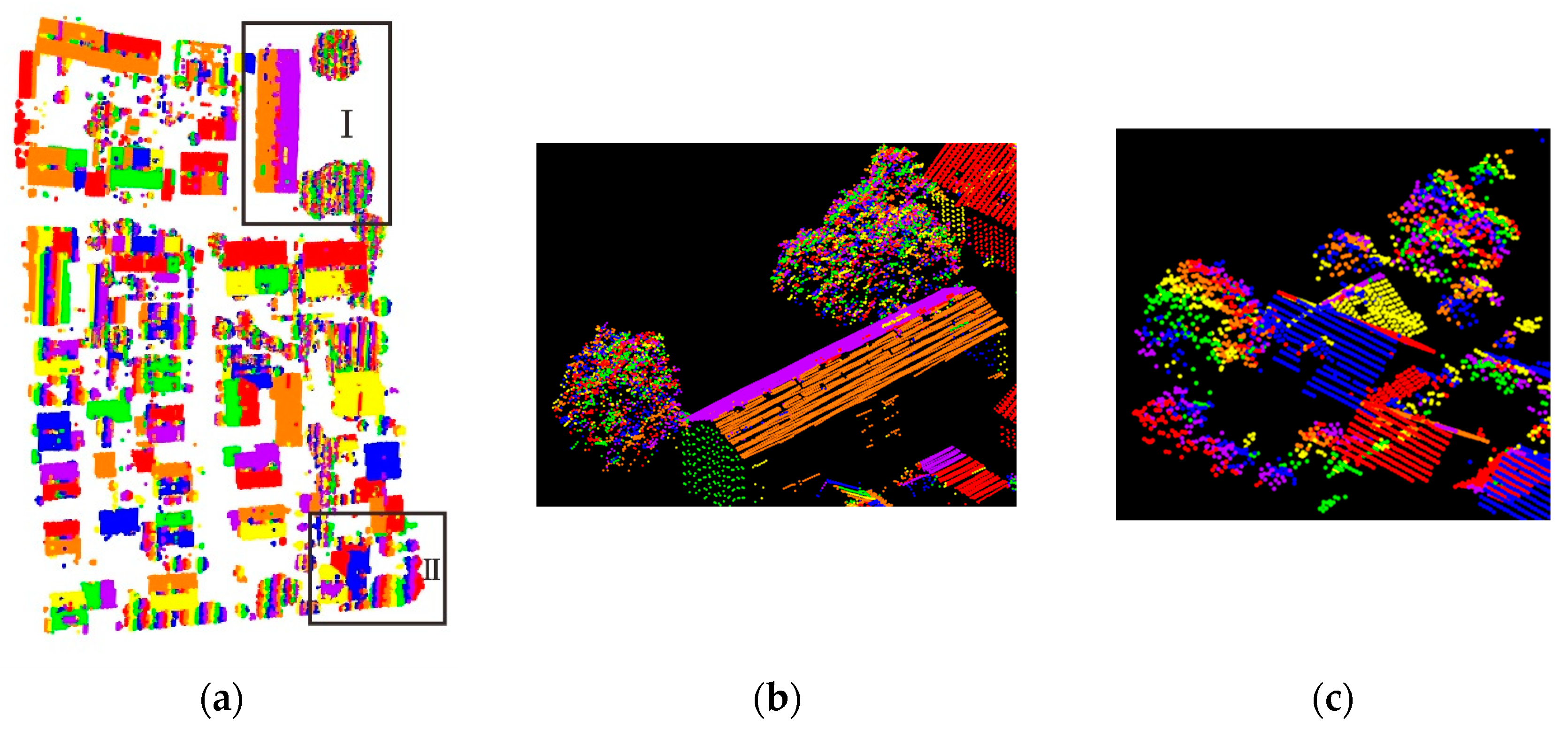
Figure 1. Flowchart of the proposed method. Filtering is first applied for removing the ground points. Then, the proposed multi-constrains graph segmentation is adopted to achieve the segmentation results. According to the geometric features, the initial building points can be obtained. Finally, an optimization step is applied to obtain the final building extraction results.
Remotesensing 13 03766 g001
Figure 2. Graph segmentation based on multi-constraints. (a) The result of graph segmentation based on multi-constraints; (b) enlarged version of the area I in (a); (c) enlarged version of the area II in (a). The colors are assigned randomly according to different segmentation objects. Different colors represent different segmentation objects.
Remotesensing 13 03766 g002
Figure 3. Building points optimization.
Remotesensing 13 03766 g003
Figure 4. The tested three datasets provided by the ISPRS. (a) Area1; (b) Area2; (c) Area3.
Remotesensing 13 03766 g004
Figure 5. Building extraction results of the proposed method. (a) Extraction results for Area1; (b) extraction results for Area2; (c) extraction results for Area3; (d) the extraction results of Area1 integrating with the corresponding orthophoto image; (e) the extraction results of Area2 integrating with the corresponding orthophoto image; (f) the extraction results of Area3 integrating with the corresponding orthophoto image. Yellow represents correctly extracted buildings ( T P ), red represents wrongly extracted buildings ( F P ), and blue represents omitted buildings ( F N ).
Remotesensing 13 03766 g005
Figure 6. Average quality comparison between the proposed method and ten other methods. (a) Per-area level; (b) per-object level. The average qualities of the ten methods are obtained from the corresponding references. The methods proposed by Maltezos et al. (2019), Doulamis et al. (2003) and Protopapadakis et al. (2016) do not provide the quality at per-object level.
Remotesensing 13 03766 g006
Figure 7. Average F1 score comparison between the proposed method and ten other methods. (a) Per-area level; (b) per-object level. The F1 score of the ten methods are obtained from the corresponding references. The methods proposed by Maltezos et al. (2019), Doulamis et al. (2003) and Protopapadakis et al. (2016) do not provide the quality at per-object level.
Remotesensing 13 03766 g007
Figure 8. Graph segmentation results with different ς . (a) ς = 1 ; (b) ς = 10 ; (c) ς = 15 ; (d) the reference segmentation results. Different object primitives are colored with different colors.
Remotesensing 13 03766 g008
Figure 9. Initial building points extraction results with different roughness threshold. (a) The threshold is 0.02; (b) the threshold is 0.04; (c) the threshold is 0.06. Yellow represents correctly extracted buildings ( T P ), red represents wrongly extracted buildings ( F P ), and blue represents omitted buildings ( F N ).
Remotesensing 13 03766 g009
Figure 10. The study areas of OpenTopography datasets. (a) The true-color image of S1; (b) the point cloud data of S1, which is colored according to different labels; (c) the true-color image of S2; (d) the point cloud data of S2, which is colored according to different labels.
Remotesensing 13 03766 g010
Figure 11. Building extraction results of OpenTopography datasets. (a) The building extraction result for S1; (b) the reference building extraction results of S1 from orthophoto image; (c) the building extraction result for S2; (d) the reference building extraction results of S2 from orthophoto image. Yellow represents correctly extracted buildings ( T P ), red represents wrongly extracted buildings ( F P ), and blue represents omitted buildings ( F N ).
Remotesensing 13 03766 g011
Table 1. Accuracy comparison of building extraction in Area1. The experimental results of the ten methods are obtained from the corresponding references. Bold font represents the highest value among the comparison results. “×” denotes that the results are not provided by the reference. Note that the methods proposed by Maltezos et al. (2019), Doulamis et al. (2003) and Protopapadakis et al. (2016) do not provide the completeness, correctness and quality at per-object level.
MethodsPer-Area (%)Per-Object (%)
CompCorrQualityF1CompCorrQualityF1
Area1Maltezos et al. (2019)79.8091.5074.4085.25××××
Doulamis et al. (2003)68.8094.0065.9079.45××××
Protopapadakis et al. (2016)92.2068.0064.3078.27××××
Awrangjeb and Fraser (2014)92.7088.7082.9090.6683.8096.9081.6189.88
Nguyen et al. (2020)90.4294.2085.6592.2783.78100.0083.7891.17
Niemeyer et al. (2012)87.0090.1079.4088.5283.8075.6065.9679.49
Wei et al. (2012)89.8092.2083.4690.9889.2097.1086.8992.98
Moussa and EI-Sheimy (2012)89.1094.7084.8791.8183.80100.0083.8091.19
Yang et al. (2013)87.9091.2081.0389.5281.1096.8078.9888.26
Gerke and Xiao (2014)91.2090.3083.0690.7586.5091.4079.9988.88
The proposed method93.0491.6185.7492.3297.2290.3488.0793.65
Table 2. Accuracy comparison of building extraction in Area2. The experimental results of the ten methods are obtained from the corresponding references. Bold font represents the highest value among the comparison results. “×” denotes that the results are not provided by the reference. Note that the methods proposed by Maltezos et al. (2019), Doulamis et al. (2003) and Protopapadakis et al. (2016) do not provide the completeness, correctness and quality at per-object level.
MethodsPer-Area (%)Per-Object (%)
CompCorrQualityF1CompCorrQualityF1
Area2Maltezos et al. (2019)87.7096.0084.6091.66××××
Doulamis et al. (2003)83.1092.3077.6087.46××××
Protopapadakis et al. (2016)90.8090.5082.9090.65××××
Awrangjeb and Fraser (2014)91.5091.0083.9091.2585.7084.6074.2085.15
Nguyen et al. (2020)93.4794.7588.8794.1178.57100.0078.5788.00
Niemeyer et al. (2012)93.8091.4086.1992.5878.6052.4045.8662.88
Wei et al. (2012)92.5093.9087.2693.1978.60100.0078.6088.02
Moussa and EI-Sheimy (2012)93.2095.4089.1994.2978.60100.0078.6088.02
Yang et al. (2013)88.8094.0084.0491.3378.60100.0078.6088.02
Gerke and Xiao (2014)94.0089.0084.2291.4378.6042.3037.9355.00
The proposed method96.8692.9390.2194.8593.3396.5590.3294.91
Table 3. Accuracy comparison of building extraction in Area3. The experimental results of the ten methods are obtained from the corresponding references. Bold font represents the highest value among the comparison results. “×” denotes that the results are not provided by the reference. Note that the methods proposed by Maltezos et al. (2019), Doulamis et al. (2003) and Protopapadakis et al. (2016) do not provide the completeness, correctness and quality at per-object level.
MethodsPer-Area (%)Per-Object (%)
CompCorrQualityF1CompCorrQualityF1
Area3Maltezos et al. (2019)88.2093.7083.2090.87××××
Doulamis et al. (2003)82.9092.9078.0087.62××××
Protopapadakis et al. (2016)96.7084.5082.2090.19××××
Awrangjeb and Fraser (2014)93.9086.3081.7089.9478.6097.8077.2387.16
Nguyen et al. (2020)91.0093.0285.1892.0083.9397.9282.4690.39
Niemeyer et al. (2012)93.8093.7088.2493.7582.1090.2075.3885.96
Wei et al. (2012)86.8092.5081.0989.5675.00100.0075.0085.71
Moussa and EI-Sheimy (2012)87.0095.2083.3490.9266.10100.0066.1079.59
Yang et al. (2013)85.2089.5077.4687.3073.2097.6071.9183.66
Gerke and Xiao (2014)89.1092.5083.1090.7775.0078.2062.3076.57
The proposed method91.5497.5989.5294.4692.1694.0987.1293.12
Table 4. Accuracy of building extraction in OpenTopography datasets.
Per-Area (%)Per-Object (%)
CompCorrQualityF1CompCorrQualityF1
S196.5499.2895.8797.8998.2598.6196.9098.43
S296.0998.3494.5697.20100.0091.4391.4395.52
Publisher’s Note: MDPI stays neutral with regard to jurisdictional claims in published maps and institutional affiliations.