
Mapping Forest Vertical Structure in Sogwang-ri Forest from Full-Waveform Lidar Point Clouds Using Deep Neural Network


Abstract
:
1. Introduction
2. Materials and Methods
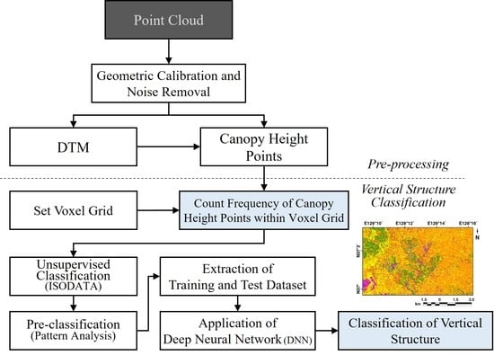
3. Methodology
3.1. Pre-Processing of LiDAR Point Clouds
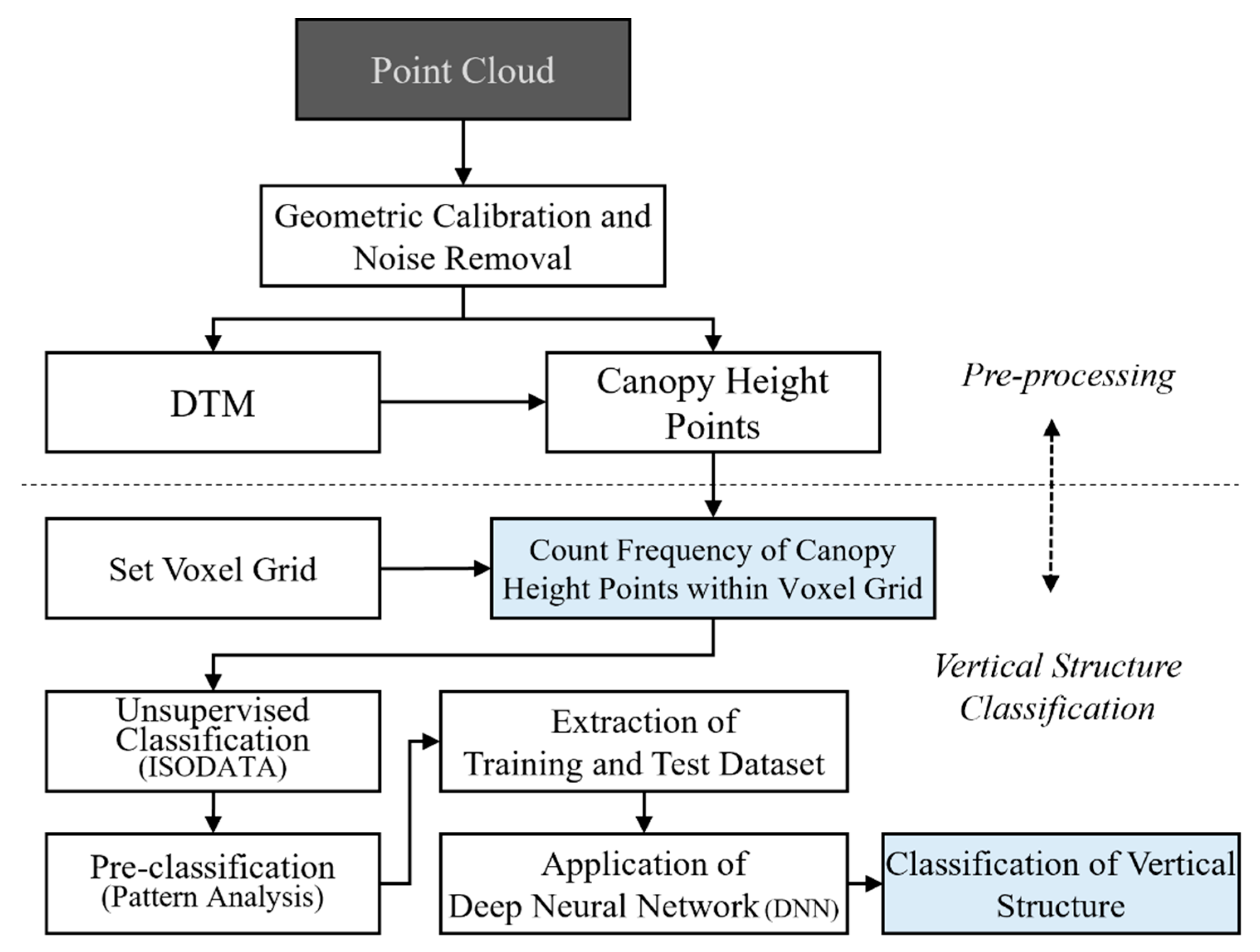
3.2. Voxel-Based Tree Point Density Mapping
3.3. Pre-Classification of Forest Vertical Structure
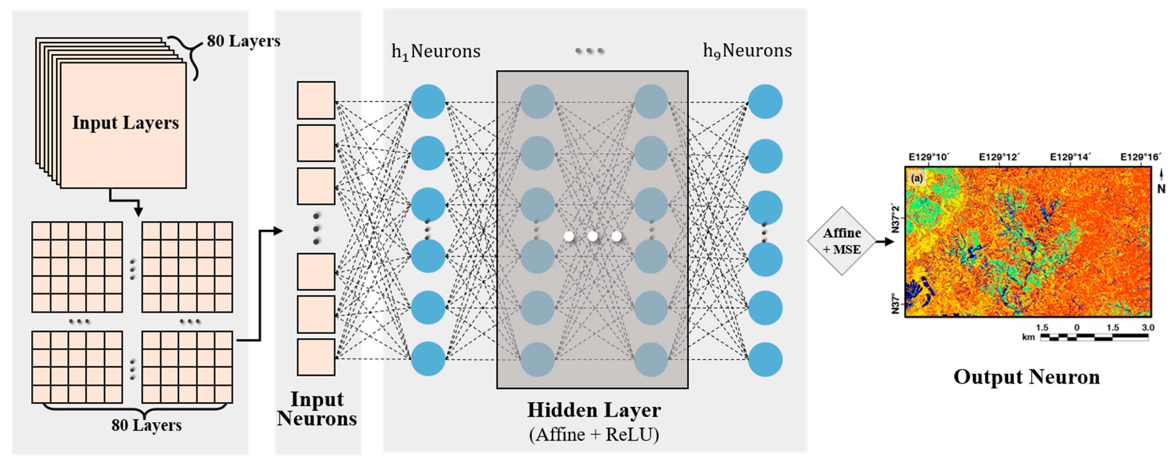
3.4. Application of Deep Neural Network
4. Results and Discussion
4.1. Pre-Processing
4.2. Voxel-Based Tree Point Density Mapping
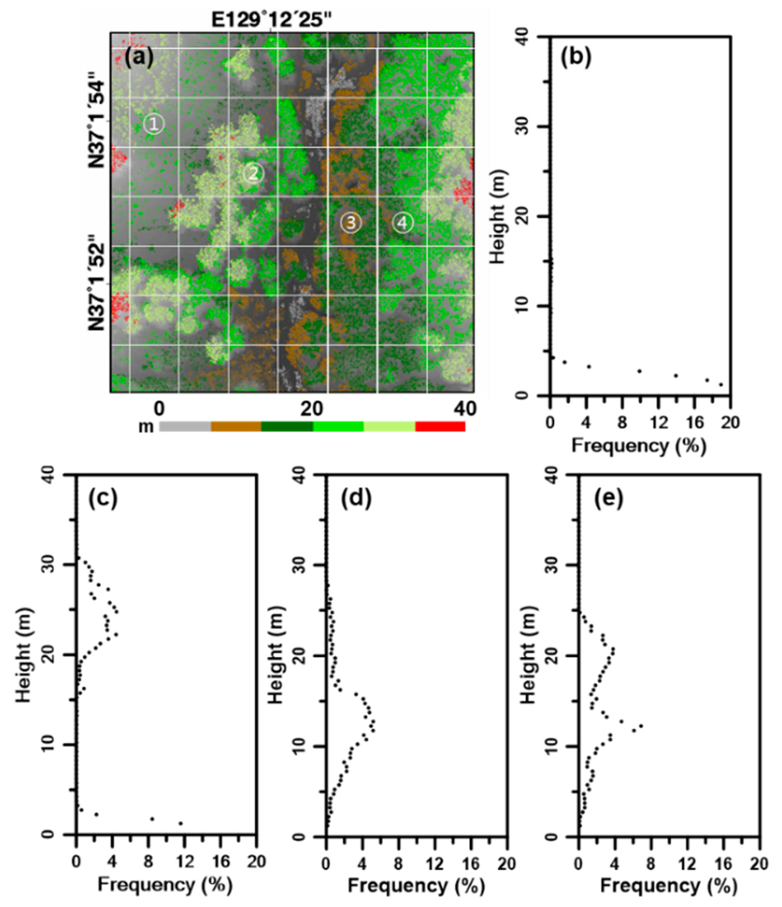
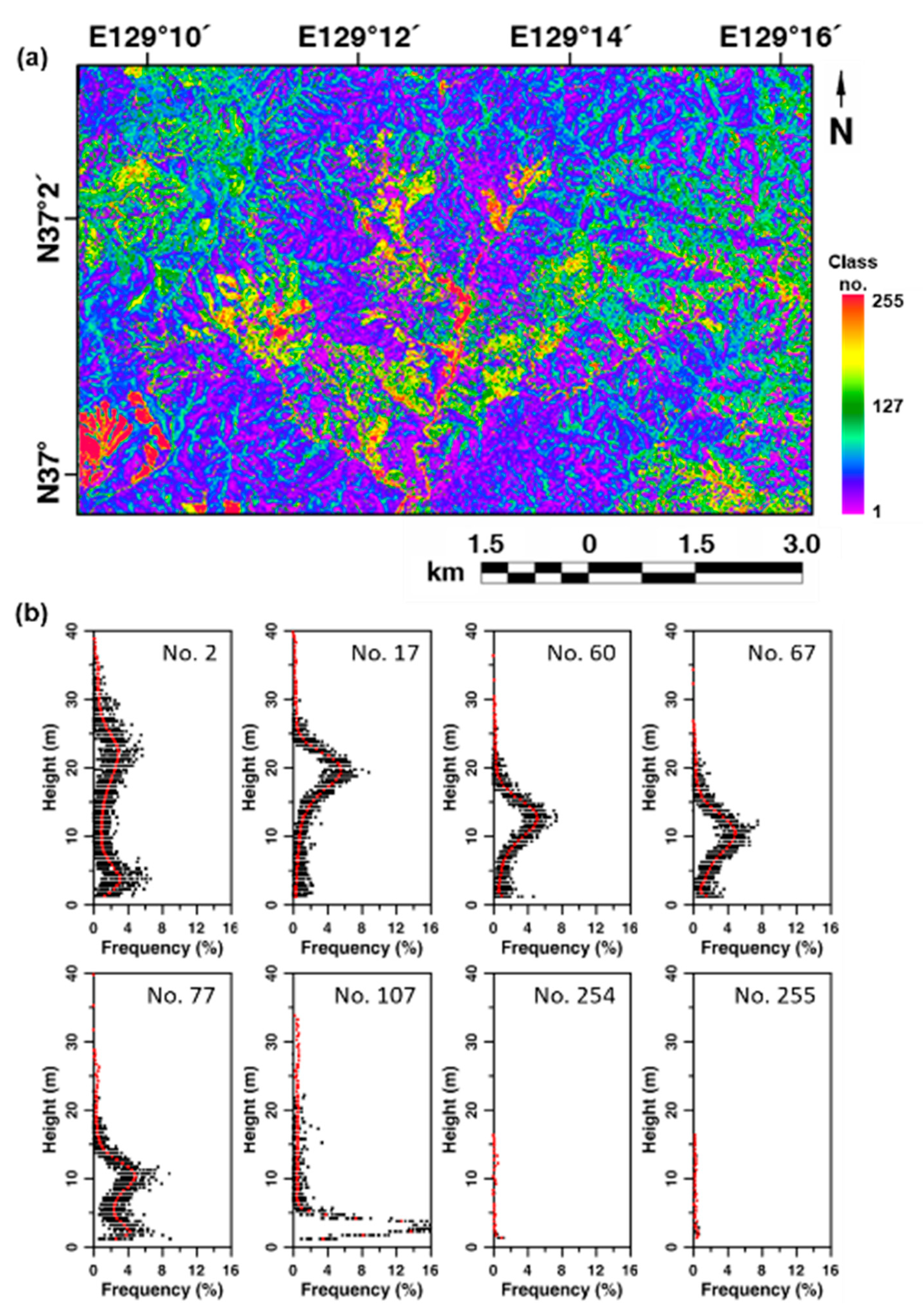
4.3. Pre-Classification of Forest Vertical Structure
4.4. Classification Map of Forest Vertical Structure
5. Conclusions
Author Contributions
Funding
Institutional Review Board Statement
Data Availability Statement
Conflicts of Interest
References
- Dennison, W.C.; Orth, R.J.; Moore, K.A.; Stevenson, J.C.; Carter, V.; Kollar, S.; Bergstrom, P.W.; Batiuk, R.A. Assessing water quality with submersed aquatic vegetation: Habitat requirements as barometers of Chesapeake Bay health. BioScience 1993, 43, 86–94. [Google Scholar] [CrossRef]
- Gardner, T.A.; Barlow, J.; Chazdon, R.; Ewers, R.M.; Harvey, C.A.; Peres, C.A.; Sodhi, N.S. Prospects for tropical forest biodiversity in a human-modified world. Ecol. Lett. 2009, 12, 561–582. [Google Scholar] [CrossRef] [PubMed] [Green Version]
- Ruiz-Jaen, M.C.; Mitchell Aide, T. Restoration success: How is it being measured? Restor. Ecol. 2005, 13, 569–577. [Google Scholar] [CrossRef]
- Tews, J.; Brose, U.; Grimm, V.; Tielbörger, K.; Wichmann, M.C.; Schwager, M.; Jeltsch, F. Animal species diversity driven by habitat heterogeneity/diversity: The importance of keystone structures. J. Biogeogr. 2004, 31, 79–92. [Google Scholar] [CrossRef] [Green Version]
- Saldaña, A.; Parra, M.J.; Flores-Bavestrello, A.; Corcuera, L.J.; Bravo, L.A. Effects of forest successional status on microenvironmental conditions, diversity, and distribution of filmy fern species in a temperate rainforest. Plant Species Biol. 2014, 29, 253–262. [Google Scholar] [CrossRef]
- Dieler, J.; Uhl, E.; Biber, P.; Müller, J.; Rötzer, T.; Pretzsch, H. Effect of forest stand management on species composition, structural diversity, and productivity in the temperate zone of Europe. Eur. J. For. Res. 2017, 136, 739–766. [Google Scholar] [CrossRef]
- Garden, J.G.; Mcalpine, C.A.; Possingham, H.P.; Jones, D.N. Habitat structure is more important than vegetation composition for local-level management of native terrestrial reptile and small mammal species living in urban remnants: A case study from Brisbane, Australia. Austral Ecol. 2007, 32, 669–685. [Google Scholar] [CrossRef]
- Anderson, H.W.; Hoover, M.D.; Reinhart, K.G. Forests and Water: Effects of Forest Management on Floods, Sedimentation, and Water Supply; Department of Agriculture, Forest Service, Pacific Southwest Forest and Range Experiment Station: Albany, CA, USA, 1976; Volume 18.
- Bonan, G.B. Forests and climate change: Forcings, feedbacks, and the climate benefits of forests. Science 2008, 320, 1444–1449. [Google Scholar] [CrossRef] [PubMed] [Green Version]
- Hoen, H.F.; Solberg, B. Potential and economic efficiency of carbon sequestration in forest biomass through silvicultural management. For. Sci. 1994, 40, 429–451. [Google Scholar]
- Gibbs, H.K.; Brown, S.; Niles, J.O.; Foley, J.A. Monitoring and estimating tropical forest carbon stocks: Making REDD a reality. Environ. Res. Lett. 2007, 2, 045023. [Google Scholar] [CrossRef]
- Seidel, D.; Fleck, S.; Leuschner, C.; Hammett, T. Review of ground-based methods to measure the distribution of biomass in forest canopies. Ann. For. Sci. 2011, 68, 225–244. [Google Scholar] [CrossRef] [Green Version]
- Segura, M.; Kanninen, M. Allometric Models for Tree Volume and Total Aboveground Biomass in a Tropical Humid Forest in Costa Rica 1. Biotropica J. Biol. Conserv. 2005, 37, 2–8. [Google Scholar]
- Lu, D.; Chen, Q.; Wang, G.; Liu, L.; Li, G.; Moran, E. A survey of remote sensing-based aboveground biomass estimation methods in forest ecosystems. Int. J. Digit. Earth 2016, 9, 63–105. [Google Scholar] [CrossRef]
- Lee, Y.-S.; Lee, S.; Jung, H.-S. Mapping forest vertical structure in Gong-ju, Korea using Sentinel-2 satellite images and artificial neural networks. Appl. Sci. 2020, 10, 1666. [Google Scholar] [CrossRef] [Green Version]
- Lee, Y.-S.; Lee, S.; Baek, W.-K.; Jung, H.-S.; Park, S.-H.; Lee, M.-J. Mapping Forest Vertical Structure in Jeju Island from Optical and Radar Satellite Images Using Artificial Neural Network. Remote Sens. 2020, 12, 797. [Google Scholar] [CrossRef] [Green Version]
- Dubayah, R.O.; Drake, J.B. Lidar remote sensing for forestry. J. For. 2000, 98, 44–46. [Google Scholar]
- Korea Forest Service. Forest Basic Statistics; Korea Forest Service: Daejeon, Korea, 2015.
- Sun, J.; Yu, X.; Wang, H.; Jia, G.; Zhao, Y.; Tu, Z.; Deng, W.; Jia, J.; Chen, J. Effects of forest structure on hydrological processes in China. J. Hydrol. 2018, 561, 187–199. [Google Scholar] [CrossRef]
- Bergen, K.; Goetz, S.; Dubayah, R.; Henebry, G.; Hunsaker, C.; Imhoff, M.; Nelson, R.; Parker, G.; Radeloff, V. Remote sensing of vegetation 3-D structure for biodiversity and habitat: Review and implications for lidar and radar spaceborne missions. J. Geophys. Res. Biogeosci. 2009, 114. [Google Scholar] [CrossRef] [Green Version]
- Wulder, M.A.; White, J.C.; Nelson, R.F.; Næsset, E.; Ørka, H.O.; Coops, N.C.; Hilker, T.; Bater, C.W.; Gobakken, T. Lidar sampling for large-area forest characterization: A review. Remote Sens. Environ. 2012, 121, 196–209. [Google Scholar] [CrossRef] [Green Version]
- Wang, Y.; Weinacker, H.; Koch, B. A lidar point cloud based procedure for vertical canopy structure analysis and 3D single tree modelling in forest. Sensors 2008, 8, 3938–3951. [Google Scholar] [CrossRef] [PubMed] [Green Version]
- Zimble, D.A.; Evans, D.L.; Carlson, G.C.; Parker, R.C.; Grado, S.C.; Gerard, P.D. Characterizing vertical forest structure using small-footprint airborne LiDAR. Remote Sens. Environ. 2003, 87, 171–182. [Google Scholar] [CrossRef] [Green Version]
- Leitold, V.; Keller, M.; Morton, D.C.; Cook, B.D.; Shimabukuro, Y.E. Airborne lidar-based estimates of tropical forest structure in complex terrain: Opportunities and trade-offs for REDD+. Carbon Balance Manag. 2015, 10, 3. [Google Scholar] [CrossRef]
- Goodwin, N.R.; Coops, N.C.; Culvenor, D.S. Assessment of forest structure with airborne LiDAR and the effects of platform altitude. Remote Sens. Environ. 2006, 103, 140–152. [Google Scholar] [CrossRef]
- Wing, B.M.; Ritchie, M.W.; Boston, K.; Cohen, W.B.; Gitelman, A.; Olsen, M.J. Prediction of understory vegetation cover with airborne lidar in an interior ponderosa pine forest. Remote Sens. Environ. 2012, 124, 730–741. [Google Scholar] [CrossRef]
- Heinzel, J.; Koch, B. Exploring full-waveform LiDAR parameters for tree species classification. Int. J. Appl. Earth Obs. Geoinf. 2011, 13, 152–160. [Google Scholar] [CrossRef]
- Liao, W.; Van Coillie, F.; Gao, L.; Li, L.; Zhang, B.; Chanussot, J. Deep learning for fusion of APEX hyperspectral and full-waveform LiDAR remote sensing data for tree species mapping. IEEE Access 2018, 6, 68716–68729. [Google Scholar] [CrossRef]
- Nie, S.; Wang, C.; Zeng, H.; Xi, X.; Li, G. Above-ground biomass estimation using airborne discrete-return and full-waveform LiDAR data in a coniferous forest. Ecol. Indic. 2017, 78, 221–228. [Google Scholar] [CrossRef]
- Lim, K.; Treitz, P.; Wulder, M.; St-Onge, B.; Flood, M. LiDAR remote sensing of forest structure. Prog. Phys. Geogr. 2003, 27, 88–106. [Google Scholar] [CrossRef] [Green Version]
- Sumnall, M.J.; Hill, R.A.; Hinsley, S.A. Comparison of small-footprint discrete return and full waveform airborne lidar data for estimating multiple forest variables. Remote Sens. Environ. 2016, 173, 214–223. [Google Scholar] [CrossRef] [Green Version]
- Cao, L.; Coops, N.C.; Hermosilla, T.; Innes, J.; Dai, J.; She, G. Using small-footprint discrete and full-waveform airborne LiDAR metrics to estimate total biomass and biomass components in subtropical forests. Remote Sens. 2014, 6, 7110–7135. [Google Scholar] [CrossRef] [Green Version]
- Wagner, F.H.; Dalagnol, R.; Tagle Casapia, X.; Streher, A.S.; Phillips, O.L.; Gloor, E.; Aragão, L.E. Regional mapping and spatial distribution analysis of canopy palms in an amazon forest using deep learning and VHR images. Remote Sens. 2020, 12, 2225. [Google Scholar] [CrossRef]
- Narine, L.L.; Popescu, S.C.; Malambo, L. Synergy of ICESat-2 and Landsat for mapping forest aboveground biomass with deep learning. Remote Sens. 2019, 11, 1503. [Google Scholar] [CrossRef]
- Lv, Q.; Dou, Y.; Niu, X.; Xu, J.; Li, B. Classification of land cover based on deep belief networks using polarimetric RADARSAT-2 data. In Proceedings of the 2014 IEEE Geoscience and Remote Sensing Symposium, Quebec City, QC, Canada, 13–18 July 2014; pp. 4679–4682. [Google Scholar]
- Hamdi, Z.M.; Brandmeier, M.; Straub, C. Forest damage assessment using deep learning on high resolution remote sensing data. Remote Sens. 2019, 11, 1976. [Google Scholar] [CrossRef] [Green Version]
- Kim, H.-Y.; Cho, H.-J. Vegetation Composition and Structure of Sogwang-ri Forest Genetic Resources Reserve in Uljin-gun, Korea. Korean J. Environ. Ecol. 2017, 31, 188–201. [Google Scholar] [CrossRef]
- Kim, J.; Kim, E.-S.; Lim, J.-H. Topographic and meteorological characteristics of Pinus densiflora dieback areas in Sogwang-ri, Uljin. Korean J. Agric. For. Meteorol. 2017, 19, 10–18. [Google Scholar] [CrossRef] [Green Version]
- Gaulton, R.; Malthus, T.J. LiDAR mapping of canopy gaps in continuous cover forests: A comparison of canopy height model and point cloud based techniques. Int. J. Remote Sens. 2010, 31, 1193–1211. [Google Scholar] [CrossRef]
- Terrasolid. TerraScan User’s Guide; Terrasolid: Helsinki, Finland, 2004. [Google Scholar]
- Popescu, S.C.; Zhao, K. A voxel-based lidar method for estimating crown base height for deciduous and pine trees. Remote Sens. Environ. 2008, 112, 767–781. [Google Scholar] [CrossRef]
- Creation and Management of Forest Resources Act. 1. Available online: https://elaw.klri.re.kr/kor_service/lawView.do?hseq=51186&lang=ENG (accessed on 25 August 2021).
- Richards, J.A.; Richards, J. Remote Sensing Digital Image Analysis; Springer: Berlin/Heidelberg, Germany, 1999; Volume 3. [Google Scholar]
- Lillicrap, T.P.; Santoro, A.; Marris, L.; Akerman, C.J.; Hinton, G. Backpropagation and the brain. Nat. Rev. Neurosci. 2020, 21, 335–346. [Google Scholar] [CrossRef] [PubMed]
- Referowska-Chodak, E. Pressures and threats to nature related to human activities in European urban and suburban forests. Forests 2019, 10, 765. [Google Scholar] [CrossRef] [Green Version]


| Forest Structure Class | Description of Profile Patterns | Representative Profile | Field Investigation | Proportion (%) | |
|---|---|---|---|---|---|
| Ground surface (Class 1) | No peak point and the frequency accelerates to the ground surface | 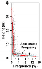 | 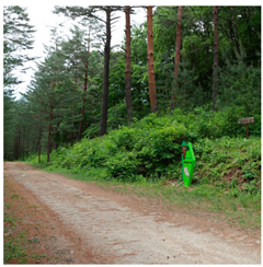 | 2.18 | |
| One-storied forest | Shrub forest (Class 2) | Only one peak point less than 5 m height | 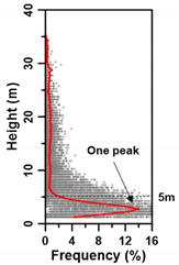 | 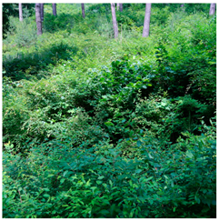 | 1.30 |
| Low height tree forest (Class 3) | Only one peak point located between 5 and 15 m height | 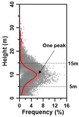 |  | 0.46 | |
| High height tree forest (Class 4) | Only one peak point located more than 15 m height |  |  | 11.67 | |
| Multi-storied forest | Shrub dominant forest (Class 5) | Two peak points, but the frequency of point below is higher than the above | 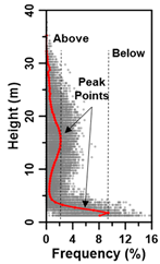 |  | 22.71 |
| Two-storied forest (Class 6) | Two peak points, but the frequency of point above is similar to or more than the below | 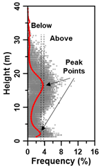 | 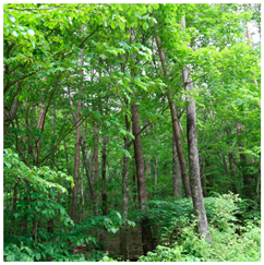 | 56.33 | |
| Mixed forest (Class 7) | A similar frequency at all heights and gradual patterns | 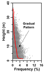 | 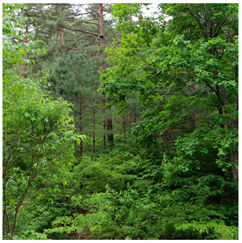 | 5.36 | |
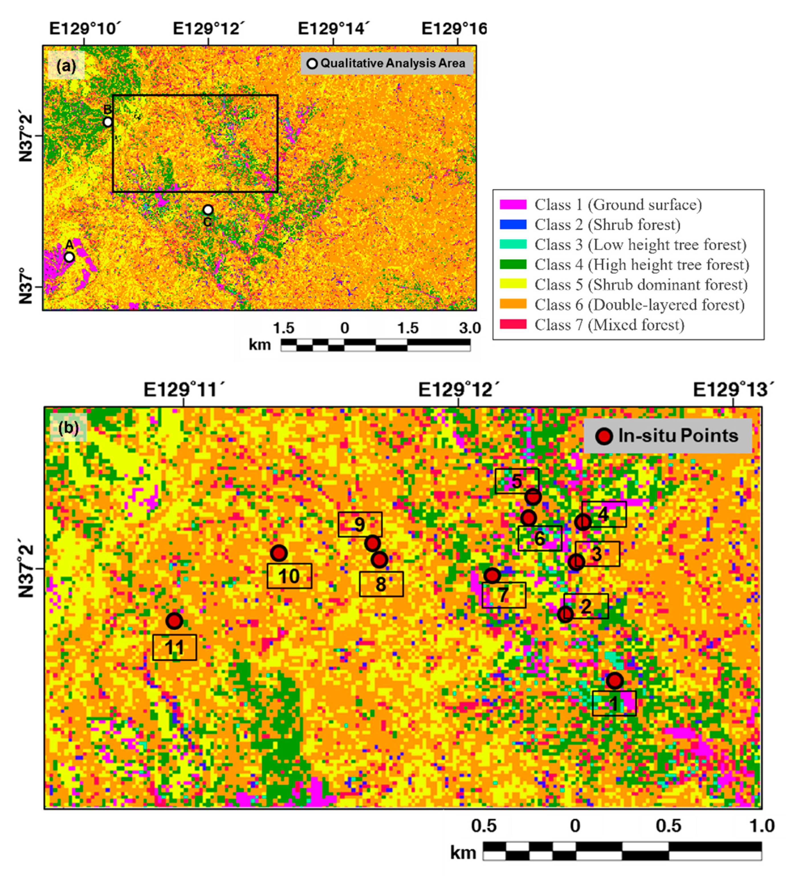
| Number of Sites | Pre-Classification Results | Field Investigation Results | Evaluation |
|---|---|---|---|
| Site 1 | Shrub dominant forest (Class 5) | 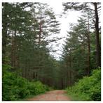 Shrub dominant forest | Matched |
| Site 2 | High height tree forest (Class 4) |  High height tree forest | Matched |
| Site 3 | Two-storied forest (Class 6) | 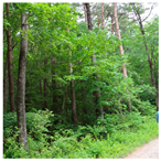 Two-storied forest | Matched |
| Site 4 | High height tree forest (Class 4) | 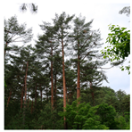 Two-storied forest | Not matched |
| Site 5 | High height tree forest (Class 4) | 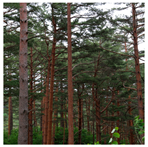 High height tree forest | Matched |
| Site 6 | Two-storied forest (Class 6) |  Shrub dominant forest | Not matched |
| Site 7 | High height tree forest (Class 4) | 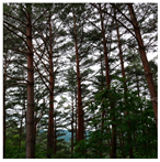 Two-storied forest | Not matched |
| Site 8 | Two-storied forest (Class 6) | 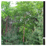 Two-storied forest | Matched |
| Site 9 | Shrub dominant forest (Class 5) | 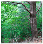 Shrub dominant forest | Matched |
| Site 10 | Mixed forest (Class 7) | 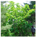 Mixed forest | Matched |
| Site 11 | High height tree forest (Class 4) |  High height tree forest | Matched |
Publisher’s Note: MDPI stays neutral with regard to jurisdictional claims in published maps and institutional affiliations. |
© 2021 by the authors. Licensee MDPI, Basel, Switzerland. This article is an open access article distributed under the terms and conditions of the Creative Commons Attribution (CC BY) license (https://creativecommons.org/licenses/by/4.0/).
Share and Cite
Park, S.-H.; Jung, H.-S.; Lee, S.; Kim, E.-S. Mapping Forest Vertical Structure in Sogwang-ri Forest from Full-Waveform Lidar Point Clouds Using Deep Neural Network. Remote Sens. 2021, 13, 3736. https://doi.org/10.3390/rs13183736
Park S-H, Jung H-S, Lee S, Kim E-S. Mapping Forest Vertical Structure in Sogwang-ri Forest from Full-Waveform Lidar Point Clouds Using Deep Neural Network. Remote Sensing. 2021; 13(18):3736. https://doi.org/10.3390/rs13183736
Chicago/Turabian StylePark, Sung-Hwan, Hyung-Sup Jung, Sunmin Lee, and Eun-Sook Kim. 2021. "Mapping Forest Vertical Structure in Sogwang-ri Forest from Full-Waveform Lidar Point Clouds Using Deep Neural Network" Remote Sensing 13, no. 18: 3736. https://doi.org/10.3390/rs13183736
APA StylePark, S.-H., Jung, H.-S., Lee, S., & Kim, E.-S. (2021). Mapping Forest Vertical Structure in Sogwang-ri Forest from Full-Waveform Lidar Point Clouds Using Deep Neural Network. Remote Sensing, 13(18), 3736. https://doi.org/10.3390/rs13183736