Diagnostics of Es Layer Scintillation Observations Using FS3/COSMIC Data: Dependence on Sampling Spatial Scale

Abstract

The basic theory and experimental results of amplitude scintillation from GPS/GNSS radio occultation (RO) observations on sporadic E (Es) layers are reported in this study. Considering an Es layer to be not a “thin” irregularity slab on limb viewing, we characterized the corresponding electron density fluctuations as a power-law function and applied the Ryton approximation to simulate spatial spectrum of amplitude fluctuations. The scintillation index S₄ and normalized signal amplitude standard deviation S₂ are calculated depending on the sampling spatial scale. The theoretical results show that both S₄ and S₂ values become saturated when the sampling spatial scale is less than the first Fresnel zone (FFZ), and S₄ and S₂ values could be underestimated and approximately proportional to the logarithm of sampled spatial wave numbers up to the FFZ wave number. This was verified by experimental analyses using the 50 Hz and de-sampled FormoSat-3/Constellation Observing System for Meteorology, Ionosphere and Climate (FS3/COSMIC) GPS RO data in the cases of weak, moderate, and strong scintillations. The results show that the measured S₂ and S₄ values have a very high correlation coefficient of >0.97 and a ratio of ~0.5 under both complete and undersampling conditions, and complete S₄ and S₂ values can be derived by dividing the measured undersampling S₄ and S₂ values by a factor of 0.8 when using 1-Hz RO data.

1. Introduction

Sporadic E (Es) layers exhibit ionization enhancements in the E region at altitudes usually between 90 and 120 km [1]. A characteristic feature of Es layers is that they are thin layers of a few kilometers’ thicknesses and a 10~1000 km horizontal extension. Over the past few decades, since the 1950s, Es layers have been extensively studied using a variety of instruments, including ionosondes, incoherent scatter radars and coherent scatter very high-frequency (VHF) radars operating from the ground and in rocket payloads with in-situ measurements. Several excellent reviews of the theories and observations of ionospheric Es layers have also been published [1,2,3,4]. It is generally believed that Es layer structure is affected by the plasma convergence effect of neutral wind shear through ion-neutral collision processes at mid and low latitudes [1]. Es layers could appear as non-uniform wave layers, a composition of irregular elongated clouds of intense ionization, or multiple layers, occurring simultaneously and separated by several kilometers within the lower E region [5]. Therefore, this gradient plasma instability can give rise to irregularities, with scale-sizes from a few tens of meters to a few kilometers, which can produce VHF/UHF radio wave scattering, and cause signal scintillations in satellite radio communication and navigation system performance [6].

The Global Positioning System (GPS) or Global Navigation Satellite System (GNSS) RO techniques provide an innovative view of the ionosphere via horizontal limb sounding from GPS/GNSS satellites to low-Earth-orbiting (LEO) satellites. There have been many successful GNSS-LEO RO missions, such as GPS/Meteorology, the Danish Ørsted, the German CHAMP (Challenging Mini-satellite Payload), the U.S.–German GRACE (Gravity Recovery and Climate Experiment), the GPS-IOX (Ionospheric Occultation Experiment), the Argentinean SAC-C (Satellite de Aplicaciones Cientificas-C), the Taiwan–U.S. COSMIC, and the Taiwan–U.S. COSMIC2. Based on these GPS/GNSS RO missions’ data, more Es layer studies have been presented [5,7,8,9,10,11]. Notably, in most of the above investigations, the criteria to identify Es events include that the peak normalized amplitude standard deviation of GPS/GNSS RO observations at E-region altitudes is higher than 0.2. However, this presents a problem for scintillation data for which the limb-viewing amplitudes of some of the GNSS-LEO RO missions were obtained at a sampling frequency less than the Fresnel frequency f_F, i.e., a sampling spatial scale larger than the first Fresnel zone (FFZ). Such undersampling had not happened in earlier Es layer investigations using incoherent scatter radars and coherent scatter VHF radars operating from the ground and in rocket payloads with in situ measurements. Thus, it is desirable to clarify the dependence on sampling spatial scale of scintillation index determination, and find a method of solving reliable scintillation indexes (S₄ and S₂) under undersampling conditions on GPS/GNSS RO observations.

In the following section, we introduce the Ryton approximation for radio wave propagations through an Es layer irregularity slab, and simulate the scintillation index S₄ and normalized signal amplitude standard deviation S₂ values, depending on the sampling spatial scale. In Section 3, we analyze the 50 Hz FS3/COSMIC RO amplitude data and the corresponding de-sampled data to prove the dependence of S₄ and S₂ determinations on sampling spatial scale. In Section 4, we present the reliability of complete S₄ and S₂ determinations using undersampling S₄ and S₂ measurements. In conclusion, we summarize the usefulness of the results.

2. Methods and Materials

When a radio wave transmitted by a satellite passes through the ionosphere, its wavefront will be distorted by irregular electron densities, i.e., plasma densities. After the radio wave has emerged from an irregularity slab, its phase front is randomly modulated. It is assumed that the deviation and the change in the refractive index over a spatial range of one wavelength and a temporal range of one wave period are slight. Under such a condition, the small-angle scattering of a layer of plasma density turbulence causes spatial and temporal fluctuations of radio wave intensity and phase, which is known as scintillation. In this study, we focus on the diagnostics of amplitude scintillation during GPS/GNSS RO observations carried out on Es layers.

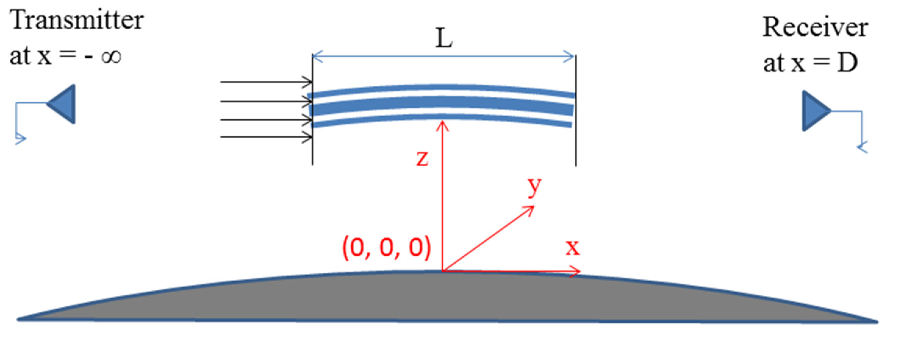
Let us assume the geometry of an Es layer scintillation problem in GPS/GNSS RO observations, as shown in Figure 1. A region of irregular electron density structures is located from x = −L/2 to x = L/2, where L could be the cutoff length of a GPS-LEO limb viewing link through an Es layer. A time-harmonic electromagnetic wave is transmitted by a GNSS satellite located at x = −∞, and it is incident on an Es layer slab at x = −L/2 and received by an LEO satellite receiver at a specific coordinate (x, ρ_t), where ρ_t = (y, z) is the transverse coordinate of wave propagation. The small-angle scattering of the scintillation phenomenon reduces the propagation equation of a wave field, where $E\hspace{0.17em}=\hspace{0.17em}u(x,\hspace{0.17em}{\rho }_t)\hspace{0.17em}\exp (-i\hspace{0.17em}k\hspace{0.17em}x)$, to the parabolic wave equation in u(x, ρ_t), as follows [12].

$$-2jk\frac{\partial u}{\partial x}\hspace{0.17em}+\hspace{0.17em}{\nabla }_t^{2}u\hspace{0.17em}=\hspace{0.17em}-k^2{\epsilon }_1(x,\hspace{0.17em}{\rho }_t)\hspace{0.17em}u\hspace{0.17em},$$

(1)

where –L/2 < x < L/2, and ${\nabla }_{t\hspace{0.17em}}^2\hspace{0.17em}=\hspace{0.17em}{\partial }^2/{\partial }_y^2\hspace{0.17em}+\hspace{0.17em}{\partial }^2/{\partial }_z^2$.

$$-2jk\frac{\partial u}{\partial x}\hspace{0.17em}+\hspace{0.17em}{\nabla }_t^{2}u\hspace{0.17em}=\hspace{0.17em}0\hspace{0.17em},$$

(2)

where x > L/2. Here, ε₁(x, ρ_t) is the fluctuating part of dielectric permittivity ε(x, ρ_t). Equations (1) and (2) are of the parabolic type, whose solutions are determined uniquely by the boundary conditions at x = −L/2 and x = L/2, respectively. Notably, the irregularity slab can be characterized by its dielectric permittivity, as follows.

$$\epsilon (x,\hspace{0.17em}{\rho }_t)\hspace{0.17em}=\hspace{0.17em}\langle \epsilon \rangle \hspace{0.17em}[1\hspace{0.17em}+\hspace{0.17em}{\epsilon }_1(x,\hspace{0.17em}{\rho }_t)]\hspace{0.17em}=\hspace{0.17em}[1\hspace{0.17em}-{\left(f_{p0}/f\right)}^{\hspace{0.17em}2}]\hspace{0.17em}{\epsilon }_0\hspace{0.17em}[1\hspace{0.17em}+\hspace{0.17em}{\epsilon }_1(x,\hspace{0.17em}{\rho }_t)]\hspace{0.17em},\hspace{0.17em}$$

(3)

and

$${\epsilon }_1(x,\hspace{0.17em}{\rho }_t)\hspace{0.17em}=\hspace{0.17em}-\frac{{\left(f_{p0}/f\right)}^2\hspace{0.17em}\left[\mathrm{\Delta }N(x,\hspace{0.17em}{\rho }_t)/N_0\right]}{1-\hspace{0.17em}{\left(f_{p0}/f\right)}^{\hspace{0.17em}2}}\hspace{0.17em}\approx \hspace{0.17em}-\frac{e^2}{4{\pi }^2\hspace{0.17em}{\epsilon }_0\hspace{0.17em}m\hspace{0.17em}{f}^2}\hspace{0.17em}\mathrm{\Delta }N(x,\hspace{0.17em}{\rho }_t)\hspace{0.17em},$$

(4)

where ΔN(x, ρ_t) is the fluctuating part of electron density, and f_p0 is the plasma frequency corresponding to the background electron density N₀. f is the radio wave frequency, i.e., GPS L1- or L2-band frequency, and is much larger than f_p0. The other constants include the electronic charge e, the electronic mass m, and the free space permittivity ε₀. Notably, ε₁(x, ρ_t) is proportional to the fluctuating part of electron density ΔN(x, ρ_t) but is in inverse proportion to the square of radio wave frequency f. In this study, we do not consider the effects of wave propagation through an elongated Es layer cloud and/or multiple Es layers. It will be interesting to work on this in future investigations.

It is now generally accepted that ionospheric electron density irregularities can be characterized by a power-law function [3,13,14,15,16]. To characterize the general power-law irregularity spectrum with spatial index p, [17] introduced a fairly general correlation spectrum, as follows.

$${\Phi }_{\mathrm{\Delta }N}(\kappa )\hspace{0.17em}=\hspace{0.17em}\frac{{\sigma }_N^2\hspace{0.17em}\Gamma \left(\frac{p}{2}\right)\hspace{0.17em}{\kappa }_0^{p-3}}{{\pi }^{3/2}\hspace{0.17em}\Gamma \left(\frac{p-3}{2}\right)}\hspace{0.17em}{\left({\kappa }^2\hspace{0.17em}+{\kappa }_0^2\right)}^{-p/2}\hspace{0.17em}\propto \hspace{0.17em}{\kappa }^{-p}\hspace{0.17em},$$

(5)

where κ₀ is the wave number of the outer scale l₀ (=2π/κ₀) in an irregularity slab, and Γ( ) is the Gamma function. The outer scale is defined as an intrinsic property of the instability that causes electron density and plasma irregularities. The power-law continuum encompasses at least three orders of magnitude in the spatial scale size [13]. Notably, the power-law spectrum is expected to be valid when its spatial scale is much less than the outer scale. In practice, it conforms to a GPS-LEO limb viewing an Es layer with a 10~1000 km horizontal extension.

Historically, the first ionospheric scintillation theory was based on the idea of wave diffraction from a phase-changing screen, and named phase screen theory [14,15,18]. This assumes that, as the radio waves propagate through an irregularity slab, to the first order, only the phase is affected by the random fluctuations in refractive index. The phase screen theory can be applied for the weak scintillations usually induced by a “thin” irregularity slab. Ref. [11] derived an Es layer thickness of 1.2 km at a peak distribution based on the 50 Hz “atmPhs” FS3/COSMIC data. Considering such an Es layer distributed at an altitude of 100 km and along the Earth’s curvature, the cutoff length of a GPS-LEO limb’s viewing link through the Es layer is approximately 160 km, taken as the value of L in Figure 1. Therefore, we consider here that the Es layer in limb viewing is not a thin irregularity slab. The effects of scattering on the field amplitude inside a limb viewing irregularity slab must be included in the treatment of the Es layer scintillation phenomenon. Earlier investigations [13,19,20] derived the Ryton approximation for the parabolic wave Equations (1) and (2), and concluded that the Ryton approximation can be applied to weak and even strong ionospheric scintillations. Using the Ryton approximation, a wave field can be presented in terms of the fluctuation of a complex phase ψ(x, ρ_t), shown as follows:

$$u\hspace{0.17em}(x,\hspace{0.17em}{\rho }_t)\hspace{0.17em}=\hspace{0.17em}{u}_0\hspace{0.17em}\exp \hspace{0.17em}[\psi (x,\hspace{0.17em}{\rho }_t)]\hspace{0.17em}=\hspace{0.17em}{u}_0\hspace{0.17em}\exp \hspace{0.17em}[\chi (x,\hspace{0.17em}{\rho }_t)\hspace{0.17em}-\hspace{0.17em}j{S}_1(x,\hspace{0.17em}{\rho }_t)]\hspace{0.17em},$$

(6)

where u₀ is the average field of u(x, ρ_t) and is a reference field with definite amplitude and phase. χ(x, ρ_t) and S₁(x, ρ_t) are referred to as the log-amplitude and the phase departure of a wave field, respectively. The general Ryton solution of the parabolic wave Equations (1) and (2) was obtained as follows.

$$\begin{array}{l}\psi (x,\hspace{0.17em}{\rho }_t)\hspace{0.17em}=\hspace{0.17em}\frac{j\hspace{0.17em}k}{2\pi (\hspace{0.17em}x+L/2)}{\displaystyle \iint {\psi }_0(-L/2,\hspace{0.17em}{\rho }_t’})\hspace{0.17em}\exp \left[\frac{-j\hspace{0.17em}k\hspace{0.17em}{\left|{\rho }_t\hspace{0.17em}-\hspace{0.17em}{\rho }_t’\hspace{0.17em}\right|}^2}{2\hspace{0.17em}(x+L/2)}\hspace{0.17em}\right]\hspace{0.17em}{d}^2{\rho }_t’\hspace{0.17em}+\hspace{0.17em}\\ \hspace{0.17em}\hspace{1em}\hspace{1em}\hspace{0.17em}\frac{k^2}{4\pi }\hspace{0.17em}{\displaystyle {\int }_{-\raisebox{1ex}{$L$}\!\left/ \!\raisebox{-1ex}{$2$}\right.}^x\frac{d\zeta }{x-\zeta }{\displaystyle \iint {\epsilon }_1(\zeta ,\hspace{0.17em}{\rho }_t’)}\hspace{0.17em}\exp \left[\frac{-j\hspace{0.17em}k\hspace{0.17em}{\left|{\rho }_t\hspace{0.17em}-\hspace{0.17em}{\rho }_t’\hspace{0.17em}\right|}^2}{2\hspace{0.17em}(x-\zeta )}\hspace{0.17em}\right]\hspace{0.17em}{d}^2{\rho }_t’}\hspace{0.17em},\hspace{0.17em}\end{array}$$

(7)

where –L/2 < x < L/2.

$$\psi (x,\hspace{0.17em}{\rho }_t)\hspace{0.17em}=\hspace{0.17em}\frac{j\hspace{0.17em}k}{2\pi \hspace{0.17em}(x-L/2)}{\displaystyle \iint \psi (L/2,\hspace{0.17em}{\rho }_t’})\hspace{0.17em}\exp \left[\frac{-j\hspace{0.17em}k\hspace{0.17em}{\left|{\rho }_t\hspace{0.17em}-\hspace{0.17em}{\rho }_t’\hspace{0.17em}\right|}^2}{2\hspace{0.17em}(x-L/2)}\hspace{0.17em}\right]\hspace{0.17em}{d}^2{\rho }_t’,\hspace{0.17em}$$

(8)

where x > L/2. Notably, ψ₀(−L/2, ρ_t) = ln u(−L/2, ρ_t) corresponds to the incident wave of the irregular slab, and ψ(L/2, ρ_t) = ln u(L/2, ρ_t) is its boundary condition at x = L/2.

In this study, we develop a plane incident wave with unity amplitude to be incident on an Es layer slab in a limb-viewing direction. The small scattering angle assumption means that the mean values of the log-amplitude and phase departures of the wave field through an Es layer slab are approximately zero, i.e., <χ> ~ <S₁> ~ 0. The power spectra for χ and S₁ are given, respectively, by [21], as follows.

$${\Phi }_{\chi }\left(0,\hspace{0.17em}{\kappa }_t\right)\hspace{0.17em}=\hspace{0.17em}\frac{\pi \hspace{0.17em}{k}^{2}L}{4}\hspace{0.17em}\left[\hspace{0.17em}1-\hspace{0.17em}\frac{2k}{{\kappa }_t^2\hspace{0.17em}L}\hspace{0.17em}\sin \left(\frac{{\kappa }_t^2\hspace{0.17em}L}{2k}\right)\hspace{0.17em}\cos \left(\frac{{\kappa }_t^2\hspace{0.17em}(x-L/2)}{k}\right)\right]\hspace{0.17em}{\Phi }_{{\epsilon }_1}\left(0,\hspace{0.17em}{\kappa }_t\right)\hspace{0.17em}\hspace{0.17em}.$$

(9)

$${\Phi }_{S1}\left(0,\hspace{0.17em}{\kappa }_t\right)\hspace{0.17em}=\hspace{0.17em}\frac{\pi \hspace{0.17em}{k}^{2}L}{4}\hspace{0.17em}\left[\hspace{0.17em}1+\hspace{0.17em}\frac{2k}{{\kappa }_t^2\hspace{0.17em}L}\hspace{0.17em}\sin \left(\frac{{\kappa }_t^2\hspace{0.17em}L}{2k}\right)\hspace{0.17em}\cos \left(\frac{{\kappa }_t^2\hspace{0.17em}(x-L/2)}{k}\right)\right]\hspace{0.17em}{\Phi }_{{\epsilon }_1}\left(0,\hspace{0.17em}{\kappa }_t\right)\hspace{0.17em}.$$

(10)

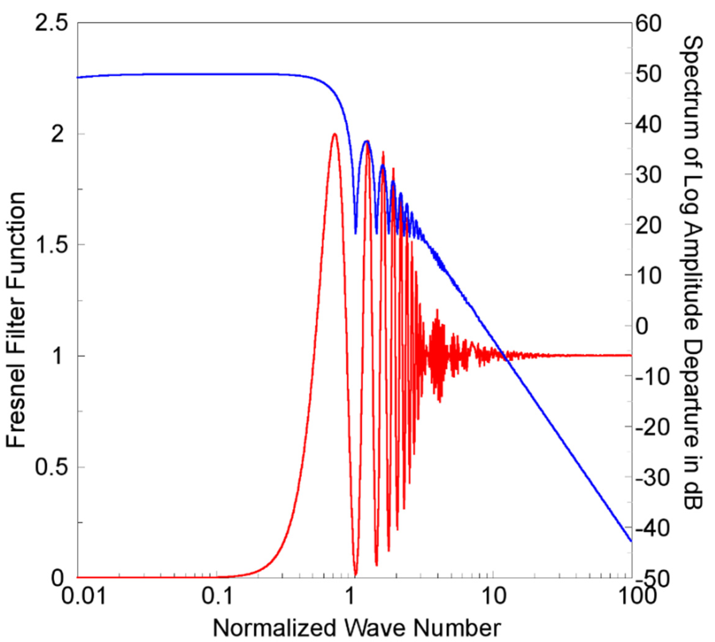
As shown in Figure 1, x is the distance from the center of an irregularity slab to the receiver on an LEO satellite, and is equal to D (~3500 km) for a GPS/GNSS RO observation on Es layers. κ_t is the wave number of a transverse spatial scale ρ_t. Notably, the spatial power spectrum of the log amplitude departure of wave field is controlled by two competing factors: a Fresnel filter function, shown as the expression in the square brackets in Equation (9), and the power-law function of dielectric permittivity or electron density fluctuation. Figure 2 shows the Fresnel filter as a function of normalized wave number κ_t/κ_F, where κ_F (=2π/D_F) is the wave number in the first Fresnel zone (FFZ) D_F (=$\sqrt{\lambda D}$=~0.8 km) corresponding to the GPS L1-band signal and a distance D of approximately 3500 km from the Es layer slab to the LEO satellite during a GPS/GNSS RO observation. The oscillatory character of the filter function is known as the Fresnel oscillation [3]. In Figure 2, the spatial power spectrum of the simulated log amplitude departure of wave field from Equation (9) is also shown at a spatial index p of 4. The spatial spectrum is generally of a power-law type with an order of p that decays as κ_t increases. It has a maximum around κ_t = κ_F, corresponding to the first maximum of the Fresnel filter function. This is consistent with an irregularity size in the order of FFZ, which is most effective in causing amplitude scintillation.

Applying the Wiener–Khinchin theorem [12] and Equations (3)–(5) and (9), the correlation of the log amplitude departure of the wave field can be derived by its spatial power spectrum, as follows.

$$\begin{array}{l}\langle {\chi }^2\rangle \hspace{0.17em}=\hspace{0.17em}{B}_{\chi }(0)\hspace{0.17em}=\hspace{0.17em}\hspace{0.17em}{\displaystyle \iint \hspace{0.17em}{\Phi }_{\chi }\left(0,\hspace{0.17em}{\kappa }_t\right)}\hspace{0.17em}{d}^2{\kappa }_t\hspace{0.17em}\\ =\hspace{0.17em}\frac{{\sigma }_N^2\hspace{0.17em}\Gamma \left(\frac{p}{2}\right)\hspace{0.17em}L}{2^{\frac{p}{2}}\hspace{0.17em}{\pi }^{\frac{p+1}{2}}\hspace{0.17em}\Gamma \left(\frac{p-3}{2}\right)}\hspace{0.17em}{\displaystyle \iint \left[1-\hspace{0.17em}\frac{1}{\pi }\hspace{0.17em}\frac{{\kappa }_f^2}{{\kappa }_t^2}\hspace{0.17em}\frac{x}{L}\hspace{0.17em}\sin \left(\pi \frac{{\kappa }_t^2}{{\kappa }_f^2}\frac{L}{x}\right)\hspace{0.17em}\cos \left(2\pi \frac{{\kappa }_t^2}{{\kappa }_f^2}\frac{\left(x-\frac{L}{2}\right)}{x}\right)\right]\hspace{0.17em}\frac{{\kappa }_0^{p-3}\hspace{0.17em}{k}^{2-p/2}\hspace{0.17em}{x}^{p/2}}{{\left(\frac{{\kappa }_t^2}{{\kappa }_f^2}\hspace{0.17em}+\hspace{0.17em}\frac{{\kappa }_0^2}{{\kappa }_f^2}\right)}^{p/2}}\hspace{0.17em}{d}^2{\kappa }_t},\end{array}$$

(11)

As a measure of amplitude scintillation, the scintillation index S₄ is most often used and is defined as a normalized variance of signal power intensity I, as follows.

$$S_4^2\hspace{0.17em}=\hspace{0.17em}\frac{\langle {\left(I\hspace{0.17em}-\langle I\rangle \right)}^{\hspace{0.17em}2}\rangle }{{\langle I\rangle }^2}\hspace{0.17em}\hspace{0.17em}.$$

(12)

Applying Ryton approximation, it is natural to suppose that the logarithmic amplitude has a normal distribution with a mean of zero because of the small angle scattering through an irregularity slab. Therefore, <χ> and <χ³> are approximately zero, and can be neglected, and <χ⁴> = 3<χ²>². Considering the moderate or strong scintillations as radio waves propagate through an Es layer’s irregularity slab, we include the first four orders of the Taylor series in our exponential functions and obtain

$$S_4^2\hspace{0.17em}=\hspace{0.17em}\frac{\langle u_0^4\hspace{0.17em}\exp (4\chi )\rangle }{{\langle u_0^2\hspace{0.17em}\exp (2\chi )\rangle }^2}\hspace{0.17em}-1\hspace{0.17em}\approx \hspace{0.17em}\frac{4\hspace{0.17em}\langle {\chi }^2\rangle \hspace{0.17em}+\hspace{0.17em}24\hspace{0.17em}{\langle {\chi }^2\rangle }^2}{1\hspace{0.17em}+\hspace{0.17em}4\hspace{0.17em}\langle {\chi }^2\rangle \hspace{0.17em}+\hspace{0.17em}8\hspace{0.17em}{\langle {\chi }^2\rangle }^2}\hspace{0.17em}.$$

(13)

Notably, the square of the S₄ value is a function of the log amplitude departure correlation of wave field, i.e., <χ²>. Equation (13) indicates that, for weak scintillations, i.e., $\langle {\chi }^2\rangle <<1$, $S_4^2~4\langle {\chi }^2\rangle$, and the S₄ value is approximately equal to double the square root of the integral of the log amplitude departure spectra in the spatial scale.

In practical situations of GPS/GNSS RO observations, the radio signals are transmitted from a GPS/GNSS satellite and received by an LEO satellite at an altitude of approximately 100 km. The projected speed v_z of the LEO satellite in the azimuth direction, i.e., the z direction in Figure 1, is approximately 3.2 km/s, which is much faster than the projected speed of the GPS/GNSS satellite and also the drift speed of the Es layer irregularities along the z direction. The temporal variations in GPS/GNSS signals received by an LEO receiver can be considered as the result of radio beam scanning over the z-direction variations of frozen Es layer irregularities. Therefore, the sampling frequency f_s on GPS/GNSS RO observations can be transferred to the wave number κ_s of the sampling spatial scale as ${\kappa }_s\hspace{0.17em}=\hspace{0.17em}2\pi \hspace{0.17em}{f}_s/v_z$. 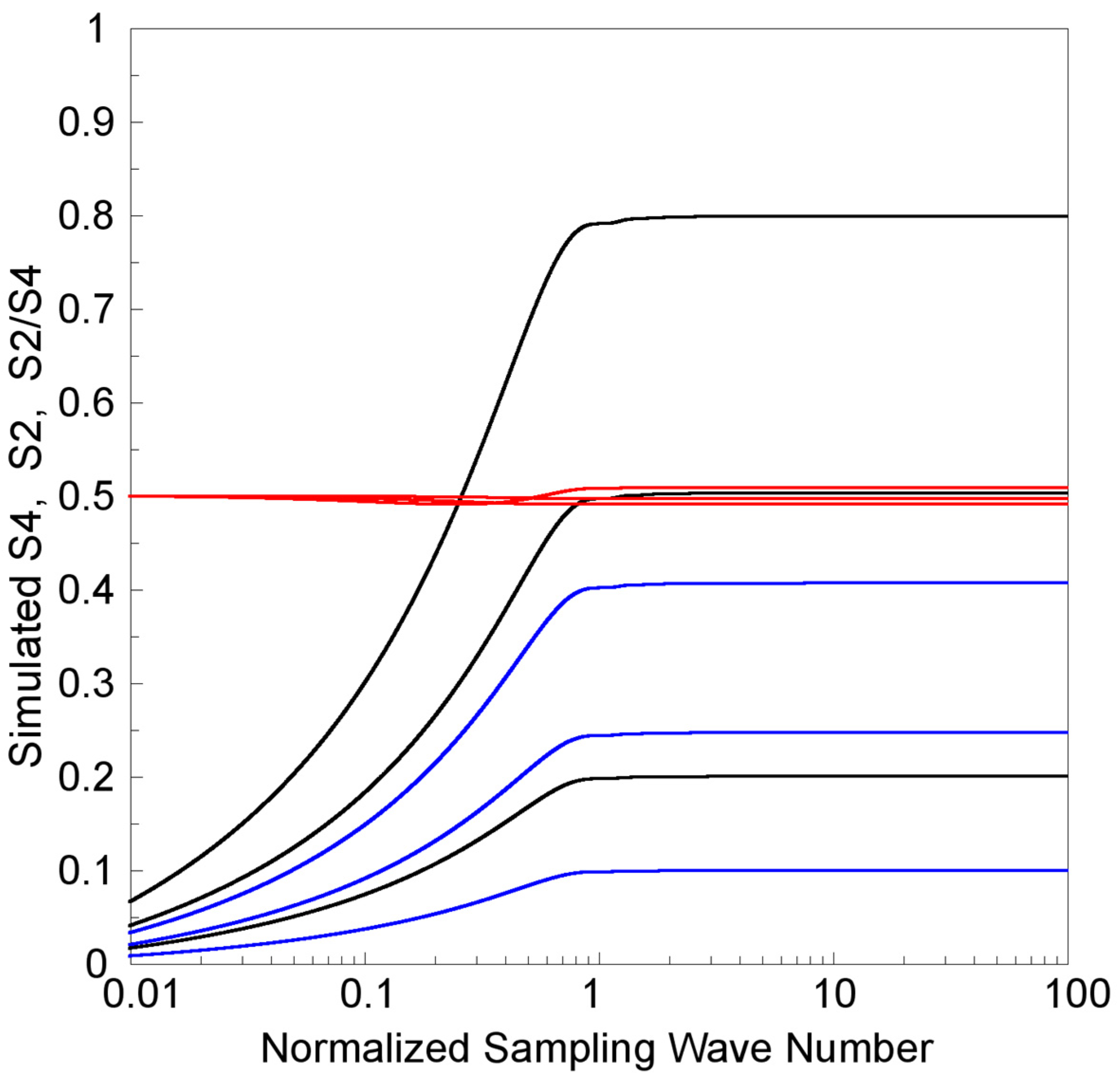Figure 3 shows three profiles of simulated S₄ values, where the saturated S₄ values are equal to 0.8, 0.5, and 0.2 separately, as functions of a normalized sampling wave number κ_s/κ_F. Three simulated S₄ profiles present results for different cases of strong, moderate, and weak scintillations, separately. Notably, when the wave number κ_s of the sampling spatial scale is larger than the wave number κ_F at the FFZ, saturation of the scintillation index S₄ becomes apparent because of the power-law spectrum of electron density fluctuation, in the order of −p. We could conclude that the S₄ values are “complete” when κ_s is larger than κ_F, i.e., the sampling spatial scale is less than the FFZ. However, for values of κ_s less than κ_F, the S₄ values decrease as the logarithm of κ_s decreases. This means that the derived S₄ values could be underestimated when the sampling spatial scale is larger than the FFZ, i.e., in “undersampling” conditions.

Another parameter used to identify the Es layer from GPS/GNSS RO observations [8,9,10,11] is the normalized signal amplitude standard deviation σ_A, which would be equivalent to the S₂ index [22]. We apply Ryton approximation to derive a wave amplitude u_a = u₀ exp(χ). Assuming that the logarithmic amplitude χ of the wave field through an Es layer slab has a normal distribution with a mean of zero, we define S₂ as follows:

$$S_2^2\hspace{0.17em}=\hspace{0.17em}\frac{\langle {\left(u_a\hspace{0.17em}-\langle u_a\rangle \right)}^{\hspace{0.17em}2}\rangle }{{\langle u_a\rangle }^2}\hspace{0.17em}=\hspace{0.17em}\frac{\langle u_0^2\hspace{0.17em}\exp (2\hspace{0.17em}\chi )\rangle }{{\langle u_0\hspace{0.17em}\exp (\chi )\rangle }^2}\hspace{0.17em}-1\hspace{0.17em}\approx \hspace{0.17em}\frac{\langle {\chi }^2\rangle \hspace{0.17em}+\hspace{0.17em}\frac{3}{2}{\langle {\chi }^2\rangle }^2}{1\hspace{0.17em}+\hspace{0.17em}\langle {\chi }^2\rangle \hspace{0.17em}+\hspace{0.17em}\frac{1}{2}{\langle {\chi }^2\rangle }^2}\hspace{0.17em}.$$

(14)

Being similar to the scintillation index S₄, the square of the normalized signal amplitude standard deviation S₂ is a function of the log amplitude departure correlation of wave field, i.e., <χ²>. For weak scintillations, i.e., $\langle {\chi }^2\rangle <<1$, $S_2^2~\langle {\chi }^2\rangle$, and the S₂ value is approximately half that of S₄ and equal to the square root of the integral of the log amplitude departure spectra in the spatial scale. Figure 3 shows another three profiles of simulated S₂ values, corresponding to three complete S₄ values equal to 0.8, 0.5, and 0.2 separately, as functions of the normalized sampling wave number κ_s/κ_F. Notably, being similar to S₄, the normalized signal amplitude standard deviation S₂ values are saturated, and are complete when κ_s is larger than κ_F. However, for the values of κ_s less than κ_F, the S₂ values decrease as the logarithm of κ_s is decreasing. This also means that the derived S₂ values are underestimated when the sampling spatial scale is larger than the FFZ. Figure 3 also shows three profiles of simulated S₂/S₄ values, corresponding to three complete S₄ values equal to 0.8, 0.5, and 0.2 separately, as functions of the normalized sampling wave number κ_s/κ_F. Notably, the three profiles of simulated S₂/S₄ ratios are mostly overlapped, and all simulated S₂ values are approximately half of the simulated S₄ values for different complete S₄ values, whenever κ_s is larger or less than κ_F.

3. Results

The FS3/COSMIC is a joint Taiwan–U.S. mission consisting of six identical LEO micro-satellites from mid-2006 to 2019. Each spacecraft carried a GPS receiver developed by the Jet Propulsion Laboratory (JPL) and utilized four GPS antennas: two limb viewing occultation antennas remotely sensing the atmosphere and low ionosphere at 50 Hz from the Earth surface up to approximately 125 km, and two slant observing antennas for precise orbit determination (POD) and remotely sensing the ionosphere at 1 Hz [23]. Therefore, the use of both limb viewing and POD antennas could produce simultaneous occultation observations consisting of two sets of 50 Hz and 1 Hz limb viewing links separately with different altitude resolutions of approximately 0.064 and 3.2 km at E-region altitudes. Both the GPS RO measurements include GPS and LEO satellite orbits, carrier excess phase and carrier signal–noise ratio (SNR) amplitudes for dual GPS L-band signals (f₁ = 1575.42 MHz and f₂ = 1227.60 MHz) at 50 Hz and 1 Hz, i.e., the “atmPhs” and “ionPhs” data, respectively. Notably, the FS3/COSMIC also provides 1 Hz amplitude scintillation S₄ data at the L1 band as the “scnLv1” data. The amplitude scintillation measurements are performed by an on-board algorithm under a Gaussian distribution assumption applied to the raw 50 Hz L1-band SNR amplitude data (Syndergaard 2006, COSMIC S4 data, from the website: http://cdaac-www.cosmic.ucar.edu/cdaac/doc/documents/s4_description.pdf, accessed on 22 August 2021). The on-board S₄ measurements are not derived by the scintillation index definition shown in Equation (12), and are thus not discussed in this study.

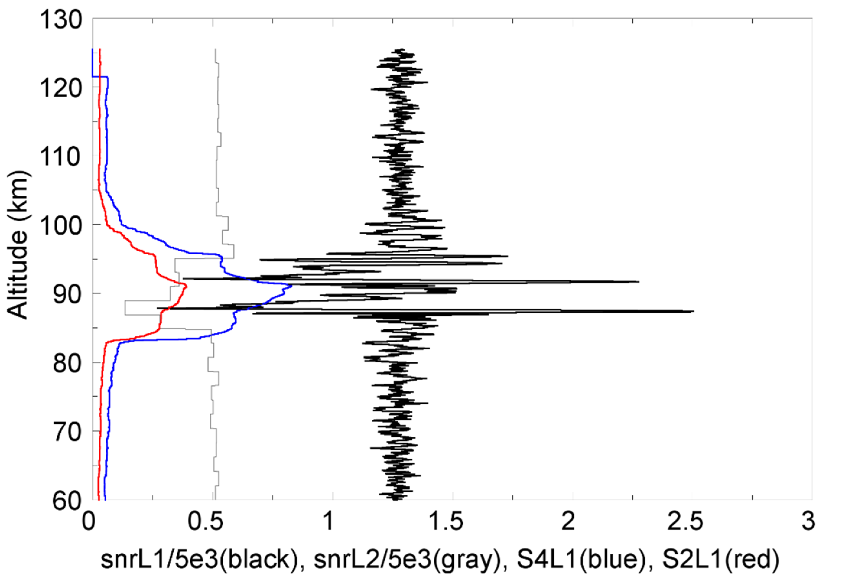
As described in the last section, the FFZ D_F of a GPS RO observation on the Es layer is approximately 0.8 km. This means that a 50 Hz limb viewing setting can be used to determine the complete scintillation index S₄ and S₂ values upon Es layer observation, but a 1 Hz limb viewing cannot. Figure 4 shows one example of FS3/COSMIC “atmPhs” (50-Hz) RO observation with an Es event recorded on 1 January 2007. As shown, significant amplitude fluctuations from L1-band signals were observed at E-region altitudes, and the corresponding S₄ and S₂ altitudinal profiles can be derived by Equations (12) and (14) separately applied to a sliding window of 4 s amplitude data. However, the L2-band signals are much weaker and have insufficient sensitivity to derive reliable S₄ and S₂ values to be shown. Notably, there is strong scintillation in the Es event, and the peak S₄ (S₂) value is 0.82 (0.39) for the GPS L1-band signals.

As mentioned, 50 Hz GPS-LEO limb viewing has a vertical sampling spatial scale of approximately 0.064 km, which is over one order less than the FFZ (~0.8 km) of the Es layer RO observation. We can perform de-sampling to obtain more sets of amplitude data at different sampling frequencies of 50/n Hz, where n = 1, 2,…, 100. The resulting one hundred sets of amplitude data can be used to derive different altitudinal S₄ and S₄ profiles using a 4 s sliding window, and obtain corresponding peak S₄ and S₂ values at sampling frequencies from 0.5 to 50 Hz, which are approximately equal to normalized sampling spatial scales κ_s/κ_F of 0.2 to 20. 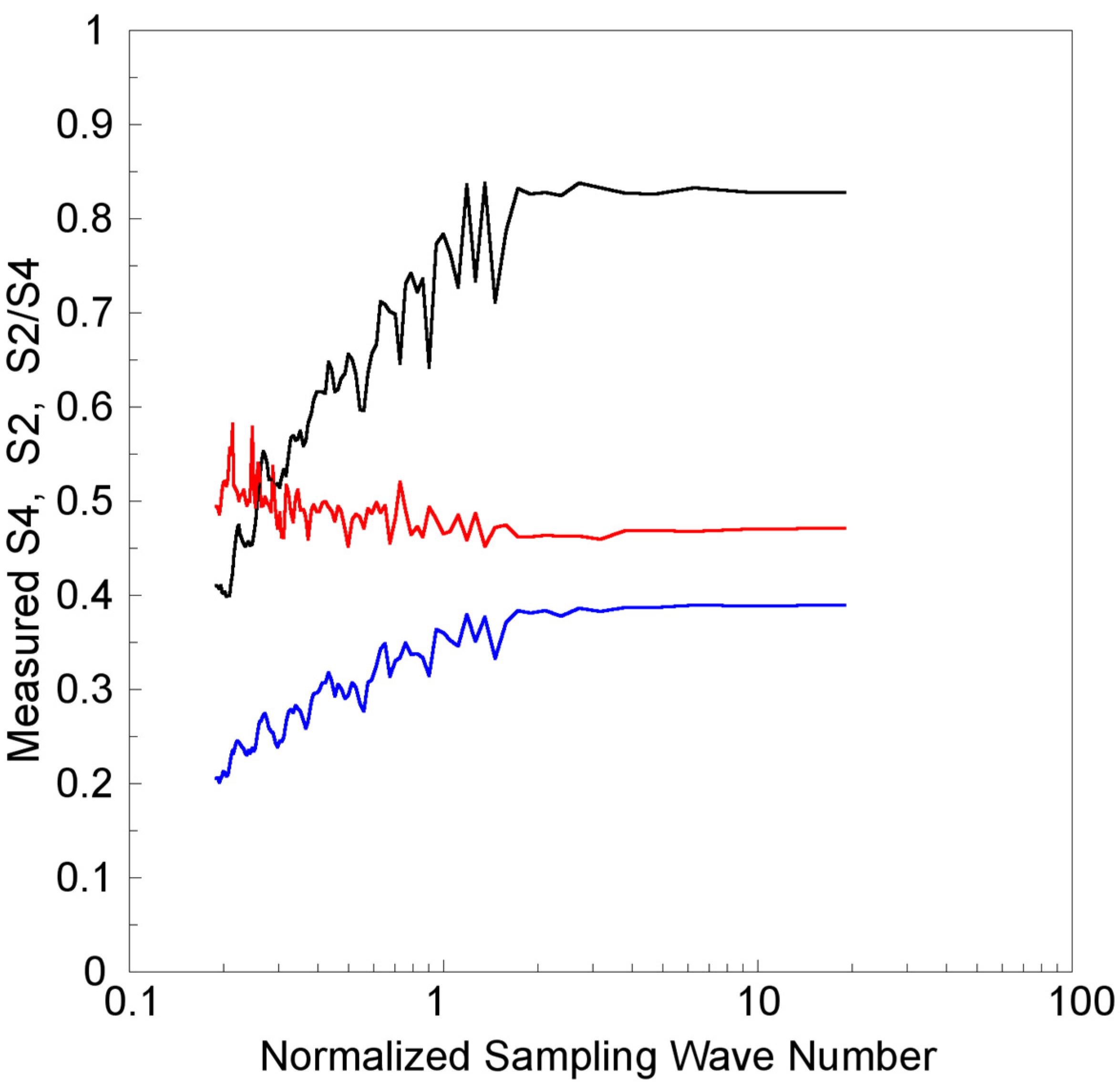Figure 5 shows the measured peaks S₄, S₂, and their ratio S₂/S₄ values as a function of κ_s/κ_F based on the FS3/COSMIC RO amplitude data, as used in Figure 4. Notably, the measured peak S₄ and S₂ profiles in κ_s/κ_F fluctuate but are mainly similar to the simulated S₄ and S₂ profiles in the strong scintillation case of a complete S₄ value of 0.8, as shown in Figure 3. The S₄ and S₂ values are saturated to ~0.8 and ~0.4, respectively, when κ_s is larger than κ_F, and, when κ_s is less than κ_F, the S₄ and S₂ values decrease in general as the logarithm of κ_s decreases. Figure 5 also shows the measured S₂/S₄ values to be more or less than 0.5 at different normalized sampling wave numbers κ_s/κ_F from 0.2 to 20, i.e., the measured S₂ values are also approximately half of the measured S₄ values whenever κ_s is larger or less than κ_F.

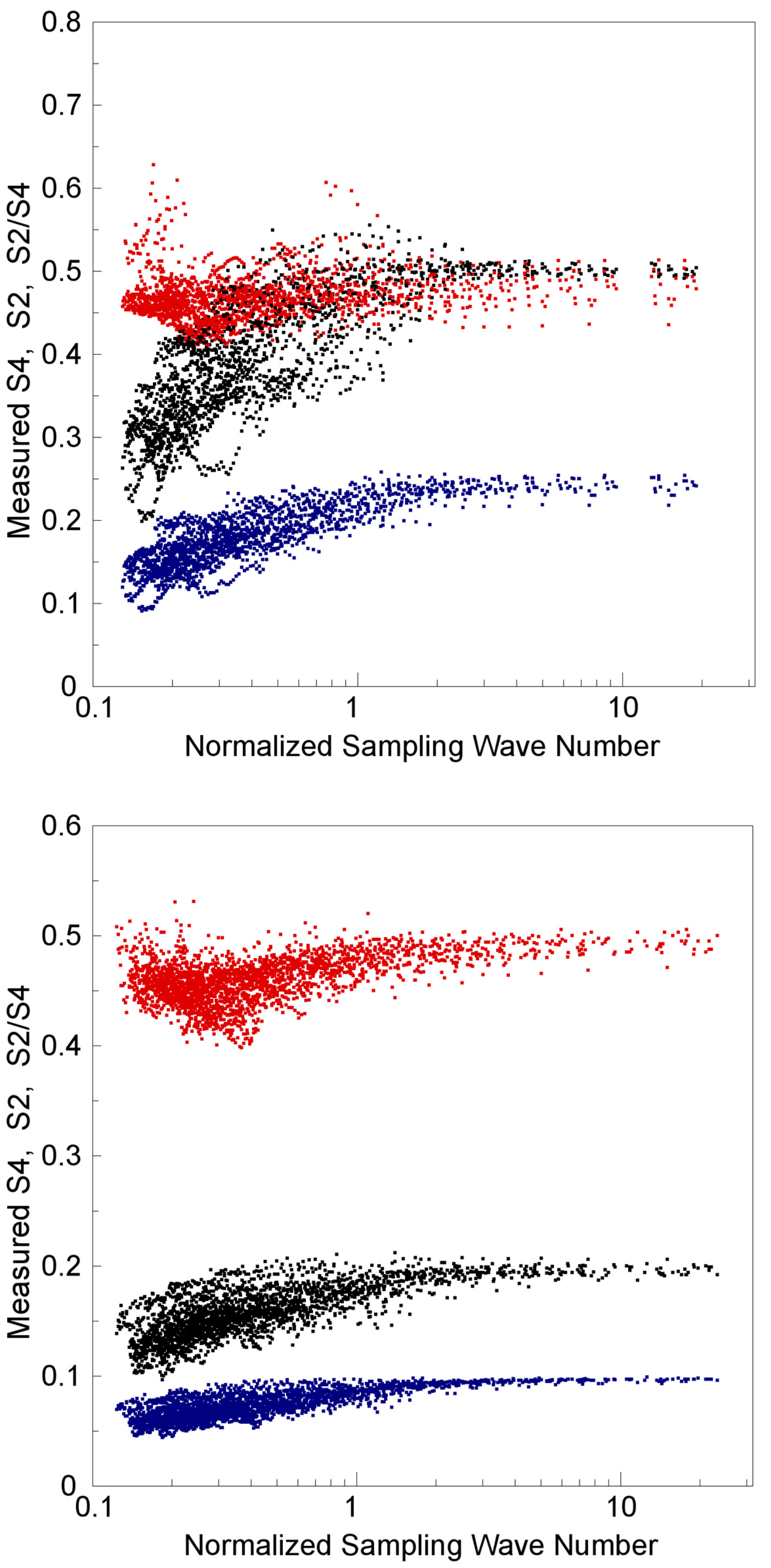
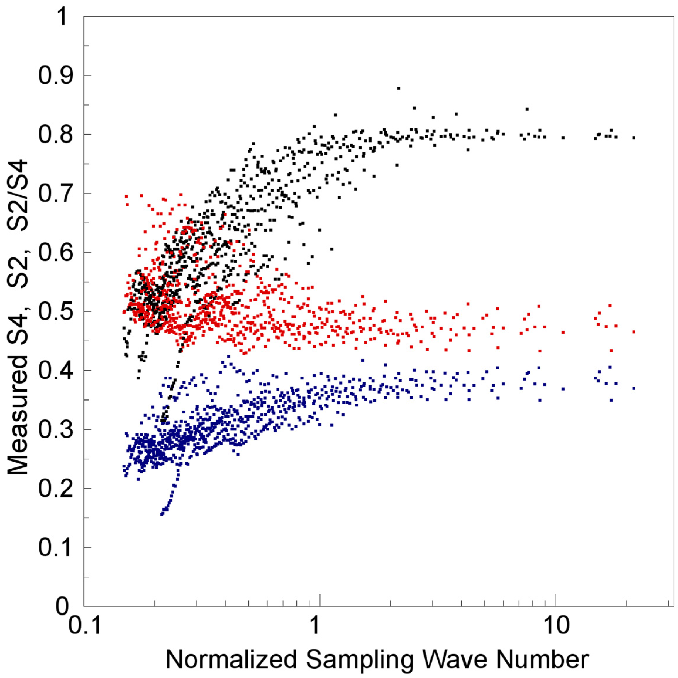
The FS3/COSMIC program performed more than one thousand complete 50 Hz GPS RO E-region observations per day from mid-2006 to the end of 2016. There were more than two thousand complete E-region observations per day in the years from 2007 to 2009, but, after 2016, the RO observation number decreased to a few hundred per day in 2019. Ref. [11] determined that around 30% of those observations were Es events, based on the criteria of its peak S₂ value (>0.2) and altitude (>80 km and less than the top altitude of each 50 Hz GPS RO observation). The local Es event occurrence rate could approach 70% during hemispheric summer seasons. To determine the dependence on the sampling spatial scale of Es layer scintillation index determinations, the top, middle, and bottom panels of Figure 6 show the peak S₄ and S₂, and their S₂/S₄ ratio values, as a function of the normalized sampling wave number for three cases of strong scintillations (complete S₄~0.8(±0.01) and 35 observations), moderate scintillations (complete S₄~0.5(±0.01) and 57 observations), and weak scintillations (complete S₄~0.2(±0.01) and 143 observations), respectively. The experimental 50 Hz FS3/COSMIC data were obtained on 1 January and 1 July 2007, and comprise 4750 GPS RO observations totally. Each RO observation was de-sampled into one hundred sets of amplitude profiles used to derived corresponding peak S₄, S₂, and S₂/S₄ values with different sampling frequencies from 0.5 to 50 Hz, i.e., normalized sampling wave numbers κ_s/κ_F from approximately 0.2 to 20. Generally, as shown in Figure 6, there was a greater spread of peak S₄, S₂, and S₂/S₄ values when sampling wave number was less. This is reasonable, because the mean error increases as its sampled number decreases, i.e., the sampling frequency decreases, and the same 4 s sampling window is used. However, the dependence on sampling spatial scale of the S₄, S₂, and S₂/S₄ values is similar to that of the simulated S₄, S₂, and S₂/S₄ profiles, shown in Figure 3, regardless of whether the scintillation cases are strong (complete S₄~0.8), moderate (complete S₄~0.5), or weak (complete S₄~0.2).

4. Discussions

Following the FS3/COSMIC mission, a follow-on program called FormoSat-7 (FS7)/COSMIC2 is in progress, with satellites launched on 25 June 2019. Similar to the FS3/COSMIC, the FS7/COSMIC2 is a six-LEO-satellite constellation mission orbiting at 24° inclination and 520~720-km altitude. It enhances GNSS receiver capability to accommodate signals from GPS and GLONASS satellites, and can provide more than 5000 RO observations per day within the region between geographic latitudes of ±40°. The large dataset from the FS7/COSMIC2 program enables precise specifications and statistical studies on equatorial and low-latitude ionospheric electron densities and irregularities. Notably, each LEO satellite of FS7/COSMIC2 also carries two limb viewing occultation antennas remotely sensing the atmosphere at 50 Hz, and another two slant observing antennas for POD and remotely sensing the ionosphere at 1 Hz. However, the altitude data of GPS/GNSS RO 50 Hz “atmPhs” are distributed between the Earth’s surface and a 60 km altitude, and do not include the E region range because of mission data storage constraints and satellite downlink bandwidth limitations [24]. This means that Es layer observations by FS7/COSMIC2 can be performed using 1 Hz “ionPhs” data only, and the S₄ and S₂ values derived by Equations (12) and (14) are underestimated under undersampling conditions and are not complete. Therefore, it is necessary to find a method for solving the underestimated scintillation indexes (S₄ and S₂).

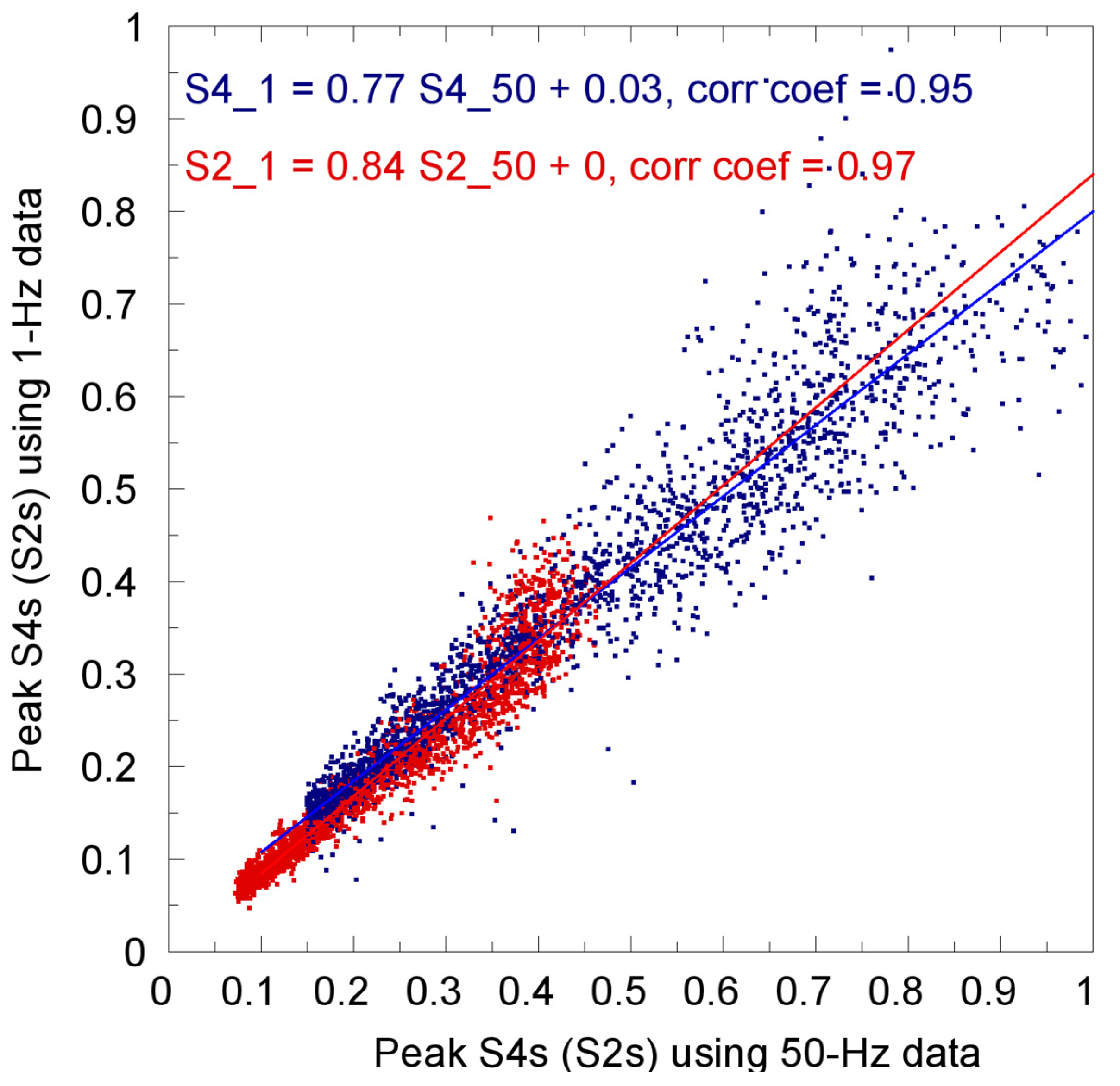
To illustrate and compare the complete and undersampled scintillation observations, Figure 7 shows two scatter plots and the corresponding least-squares fitting lines for the measured peak S₄ and S₂ values using 1 Hz FS3/COSMIC data versus the peak S₄ and S₂ values measured using 50 Hz FS3/COSMIC data, respectively, on E and Es layer observations. The experimental FS3/COSMIC data were recorded on 1 January and 1 July 2007, and the 1 Hz amplitudes have been de-sampled from the 50 Hz amplitudes of “atmPhs” data. The results show that the peak S₄ (S₂) measurements of E and Es layer observations using 50 Hz and de-sampled 1 Hz amplitude data have very high correlation coefficients of 0.95 (0.97). Meanwhile, from the least-squares fitting line equations shown in Figure 7, we see that the underestimated S₄ (S₂) values derived from the 1 Hz data have a ratio of 0.77 (0.84) to the complete S₄ (S₂) values derived from 50 Hz data. The strong correlations prove the reliability of complete S₄ and S₂ determinations using undersampled S₄ and S₂ measurements and corresponding sampling frequency or spatial scale information. Notably, the normalized spatial wave number κ_s/κ_F is approximately 0.4 at a limb-viewing sampling rate of 1 Hz on the E or Es layer RO observations. The resulting ratio of 0.77 (0.84) is close to the ratio of ~0.8 for the simulated S₄ (S₂) value (at a κ_s/κ_F of 0.4, as shown in Figure 3) to the complete S₄ (S₂) value, regardless of whether the scintillation cases are strong (complete S₄~0.8), moderate (complete S₄~0.5), or weak (complete S₄~0.2). Furthermore, as shown in Figure 7, the measured complete S₂ values are distributed from 0.07 to 0.5, approximately half of the measured complete S₄ distribution range from 0.15 to 1.0. 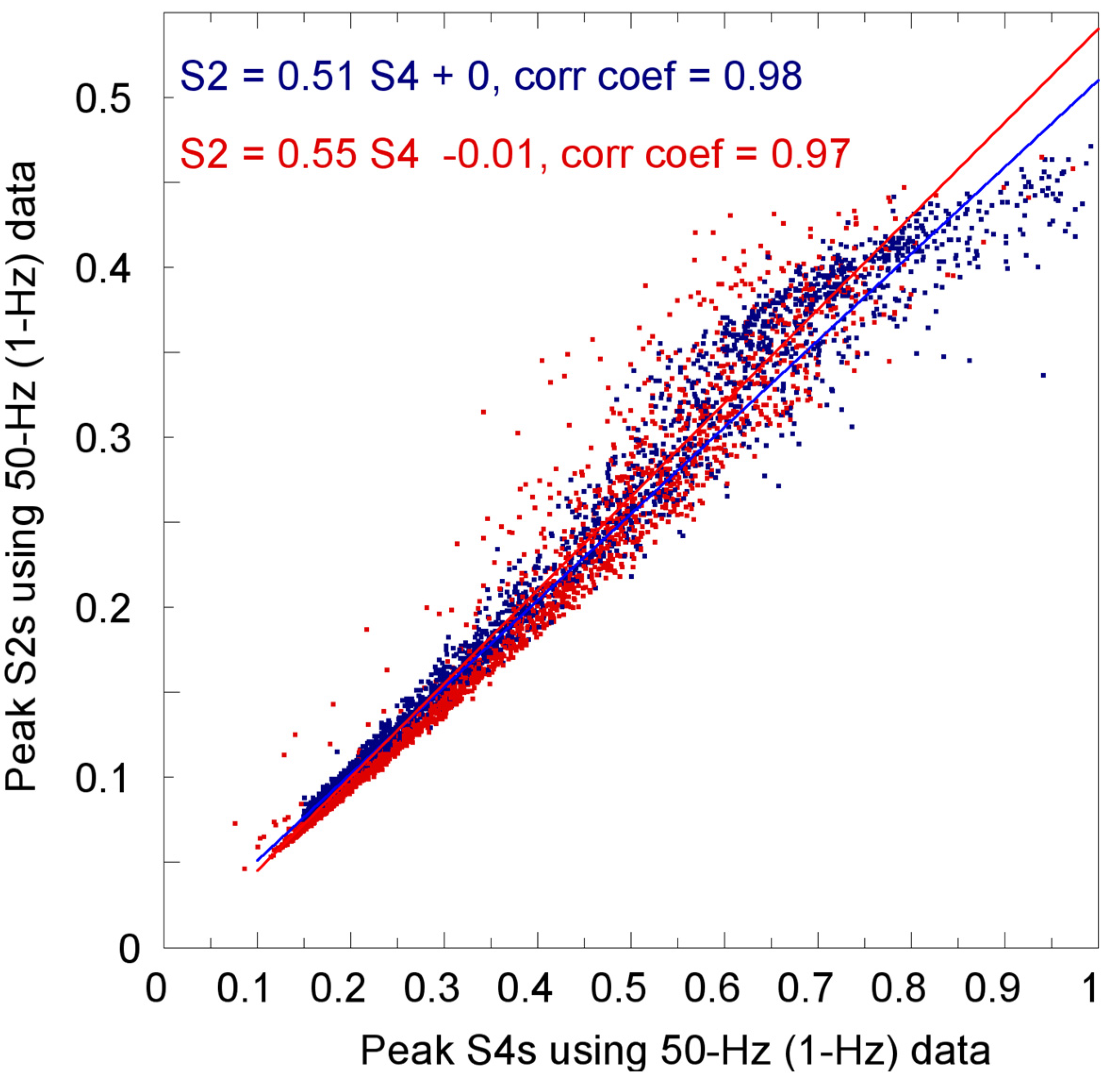Figure 8 shows another two scatter plots and the corresponding least-squares fitting lines for the peak S₂ values versus peak S₄ values measured using 50 Hz and de-sampled 1 Hz FS3/COSMIC “atmPhs” data separately in E and Es layer observations. The experimental data are the same as those used in Figure 7. The results show that the peak S₂ versus S₄ measurements for the E and Es layers have very high correlation coefficients of 0.98 and 0.97 using 50 Hz and de-sampled 1 Hz amplitude data, respectively. Meanwhile, from the least-squares fitting line equations shown in Figure 8, we see that the slopes of both fitting lines, i.e., the mean ratios of peak S₂ to S₄ values, are approximately equal to 0.5, which is the same as the simulated S₂/S₄ values shown in Figure 3. This means that the scintillation index S₄ and the normalized signal amplitude standard deviation S₂ measurements have high correlations with the determined ionospheric scintillation level.

5. Conclusions

The diffraction theory of wave propagation in a stationary random medium establishes a connection between the spatial spectrum of ionospheric electron density fluctuations and the power spectrum of observed signal intensities, and therefore the amplitude scintillations. We have reported in this paper on the relevant theories and FS3/COSMIC experiments of radio wave scintillations of Es layer RO observations. The theoretical results show that applying Ryton approximation to radio wave propagations through an Es layer irregularity slab can provide reasonable descriptions of weak-, moderate-, and strong-amplitude scintillations. We conclude that a GPS RO scintillation observation is complete when the sampling spatial scale is less than the FFZ, otherwise it is a case of undersampling. It is shown that the simulated results are consistent with interpretations of FS3/COSMIC RO scintillation index estimates in terms of the different sampling frequencies. It is useful to clarify the dependence of the determination of the scintillation index on the sampling spatial scale, and find a method for solving complete scintillation indices (S₄ and S₂) under undersampling conditions.