Abstract
Thermal inertia, which represents the resistance to change in temperature of the upper few centimeters of the surface, provides information to help understand the surficial geology and recent processes that are potentially still active today. It cannot be directly measured on Mars and is therefore usually modelled. We present a new analytical method based on Apparent Thermal Inertia (ATI), a thermal inertia proxy. Calculating ATI requires readily available input data: temperature, incidence angle, visible dust opacity, and a digital elevation model. Because of the high spatial resolution, the method can be used on sloping terrains, which makes possible thermal mapping using THEMIS in nearly any area of Mars. Comparison with results obtained by other approaches using modeled data shows similarity in flat areas and illustrates the significant influence of slope and aspect on albedo and diurnal temperature differences.
1. Introduction
The thermal inertia of surface materials is related to their physical properties, complementing other datasets for geological interpretation. Thermal inertia for a given rock composition primarily depends on density, but is subject to huge variations that depend on the rock temperature, porosity, and cementation, the increase of which results in increased thermal inertia [1]. From a geological point of view, thermal inertia, therefore, depends on rock composition and thermophysical properties; however, for a sloping surface subject to weathering, it will be heavily modulated by slope processes affecting porosity and cementation. Thermal inertia helps to understand the surficial geology and recent processes that are potentially still active today on Mars. Fine particles (dust) have low thermal inertia, and it increases for particles of sand size, then for duricrust, rock fragments, and combinations of these materials. An effective particle size of the surface can be inferred from thermal inertia values from laboratory-derived relationships between particle size and conductivity [2].
Thermal inertia represents the resistance to change in temperature of the upper few centimeters of the surface throughout the day [2]. Thermal inertia (J m−2 K−1s−1/2) in SI units is defined as:
and is related to thermal conductivity k (W m−1 K−1), density p (kg m−3), and heat capacity C (J kg−1 K−1) of the rock. Variations in thermal inertia on Mars were demonstrated to principally arise from variations in thermal conductivity [3]. Because direct measurement of thermal inertia on Mars is not possible, thermal inertia modelling has become common ([2,4,5,6,7,8,9,10,11,12,13,14,15,16]) including apparent thermal inertia (ATI), and differential apparent thermal inertia (DATI) ([10,17,18,19,20,21,22,23,24,25,26]).
ATI was introduced by Price [27], who developed a model to relate thermal inertia to parameters measurable by remote sensing. Price [17] retrieved the relationship between ATI and P and suggested a possibility to use ATI instead of P, due to the P–ATI direct relationship, confirmed also by Kahle et al. [28]:
where α and β represent a scaling factor and an offset in Price [17]. This is recommended especially in aridic climates, such as the current climate on Mars, where β related to atmospheric humidity can be neglected. Alpha depends on solar geometry factors. Thus, ATI incorporates the functional dependence on albedo, day–night temperature difference, latitude of the point of interest, and solar declination, as these factors influence the estimate of P.
ATI approximates thermal inertia [17,27]. ATI values are directly proportional to the P as proposed in the empirical formula introduced by Price [17,27], and Khale [28,29] implying thermal inertia units (cal m−2 K−1 s −1/2) inherited by ATI (see Price [17] for the formula derivation). As the traditional cal m−2 K−1 s −1 units are now rarely used, we have converted them to the SI units (J m−2 K−1 s −1/2) by multiplying them by 41855 (calorie to joule conversion). ATI is a useful option for space objects because it can be directly generated from the remote sensing data without additional modelling, as shown in the equation:
where ΔT (K) is the diurnal temperature difference (daytime–nighttime; non-corrected), and A is the Lambertian albedo. On Mars, ΔT can be obtained from Thermal Emission Imaging System (THEMIS) images. Temperature was taken at the local time on Mars. Daytime images are those with a local time of 08:00–20:00, and nighttime images are those with a local time of 00:00–07:59. The reflected intensity of a Lambertian surface is isotropic, being independent of the view zenith and relative azimuth angles. It is simply related to the incident flux [30].
Topography is an important factor in thermal inertia calculations because the incident thermal energy received by a given slope depends on its orientation and inclination. Many areas have slopes steeper than 10° on Mars. Thus, slope affects local inferred albedo and temperature. Spacecraft sensors record the angle of incidence radiation on a horizontal surface, but slope inclination and orientation are neglected. This results in albedo (and temperature) either over- or underestimated. For instance, if the incidence angle on the flat surface is 40°, and the sun shines from the south, then for a south-facing 30° slope, the actual incidence angle (i) is only 10° and the resulted albedo is lower by ~20% than it would be if the surface was horizontal. By incidence angle, we mean the angle between a ray incident on a horizontal surface and the line perpendicular to that horizontal surface at the point of incidence.
Slopes have been accounted for in several previous thermal inertia investigations. Some local studies have used KRC modelling [5,6,7], where K is for conductivity, R for density, and C for specific heat, to compute thermal inertia from THEMIS brightness temperature on sloping terrain [20,21]. The brightness temperature function converts all available THEMIS radiance bands to the blackbody temperature for the equivalent radiance integrated over each THEMIS bandpass. The authors of [2] investigated the effect of slope on thermal inertia by KRC modelling, but could not take slopes into account in global mapping due to the unavailability of global high-resolution slope data. They found, however, that for geological applications, thermal inertia derivation should take the slope angle into account when they are more than ~10°. Many geological objects are exposed on surfaces that are steeper than 10° (graben fault scarps, wrinkle ridge slopes, caldera rims, river channel benches, wind-eroded gullies, impact crater rims, and many others), which makes it necessary to develop robust approaches to determine high-resolution thermal inertia adapted to slopes above 10°. To fill this gap, we created the ATI-based method with a high spatial resolution and implemented a topography correction that makes it possible to account for steep slopes (provided that incidence angle < 79°). It is based on a mathematical algorithm that can be readily used. The method is described in Section 2. A tutorial is provided in Supplementary File S1.
2. Method and Datasets
Apparent thermal inertia primarily requires the determination of albedo and temperature (Equation (3)). Solar geometry, dust opacity, topography, and atmosphere thermal emission during nighttime influence albedo and/or temperature.
2.1. Albedo
Albedo A (Equation (3)) is obtained from Mars Reconnaissance Orbiter’s Context Camera (CTX) data. At the global scale, TES data, of resolution ~3000 m/pixel, is enough, but for detailed geologic interpretations, higher spatial resolution is required. CTX data, of resolution ~6 m/pixel, are appropriate.
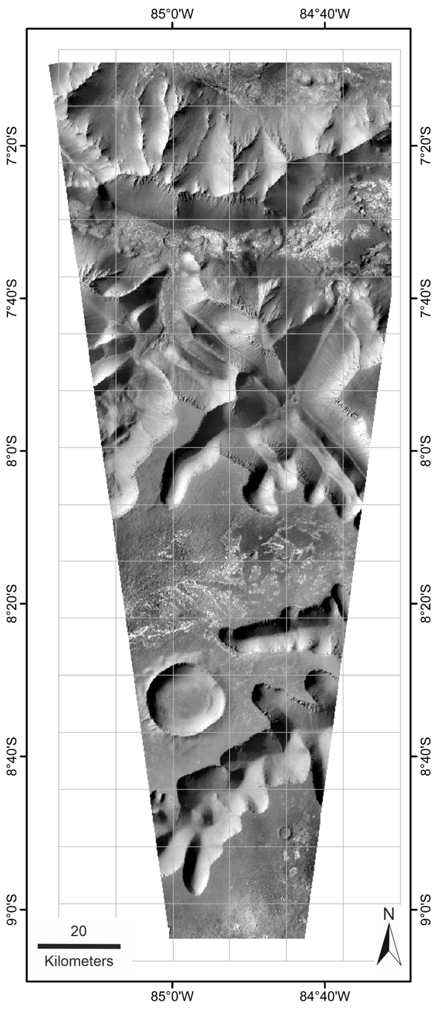
The CTX albedo, which is a Lambert albedo, is collected from a wavelength range of 500–800 nm [31]. This is smaller than the bolometric albedo of TES collected from a wavelength range of 300–2900 nm [32]. To evaluate these differences, Bell et al. [33] systematically compared the CTX albedo with bolometric albedo from the TES instruments. They proposed that the CTX-based albedo gives results ~15% lower than from the TES albedo. The albedo values provided here account for this correction proposed by Bell et al.—this factor was included in all our calculations. However, we have verified the uncertainty related to this approximation based on a mosaic of two CTX images of the Valles Marineris area (Figure 1). Their spatial resolution is degraded to 8 ppd (see Figure 1) to obtain the TES albedo map resolution. We found that there is still a difference between the CTX-derived and TES-derived albedos, which is on average 8% (Figure 2a). However, this leads to an ATI difference of only 1.5% (Figure 2b).
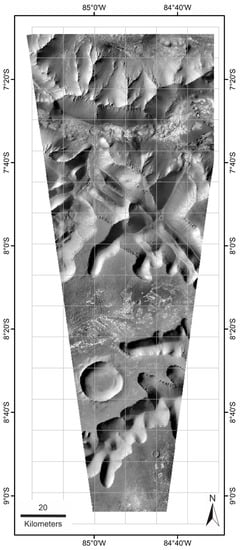
Figure 1.
Mosaic of MRO/CTX images (P01_001351_1717_XI_08S084W, P01_001417_1718_XI_08S085W) used to evaluate CTX capability at determining albedo. Grid line spacing is 8 pixels per degree (ppd), similar to the TES albedo map available at https://www.mars.asu.edu/data/tes_albedo/ (accessed on 14 September 2021). Average CTX and TES albedo are calculated for the TES pixels that are entirely located within the area covered by the CTX images.
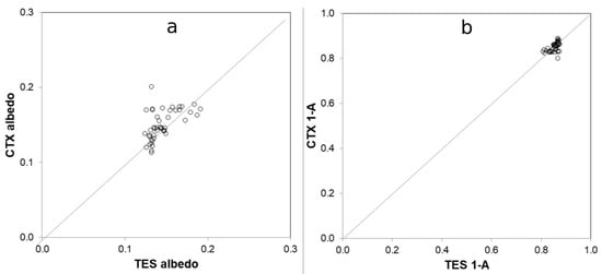
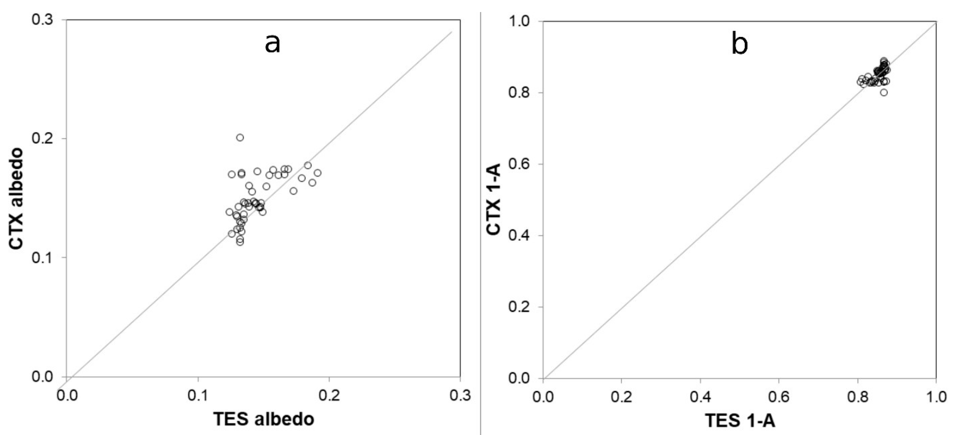
Figure 2.
(a) CTX vs. TES albedo for the 8 ppd grid pixels displayed in Figure 1; (b) comparison between 1-A (which is directly proportional to ATI, Equation (3)) for the CTX and TES data. CTX albedo is on average 8% higher than TES albedo (a), which implies CTX-calculated ATI would be 1.5% than TES-based ATI (b).
The CTX images are pre-processed using the PILOT software (http://pilot.wr.usgs.gov/, accessed on 14 September 2021). PILOT follows the ISIS [34] procedures: spiceinit (updates camera pointing information), ctxcal (applies radiometric calibration), ctxevenodd (removes even-odd detector striping), and cam2map (projects from camera space to map space). The output represents the ratio of reflected radiation (IR) to solar flux (F). Albedo is the ratio of reflected radiation (IR) to incident radiation (II):
To obtain II, the cosine of the solar incident angle (cosiCTX) is multiplied by the solar flux [33]:
where Equation (5) develops to:
Equation (6) enables calculating on a flat surface. For calculation on an inclined surface, the following correction of against topography characteristics (slope angle, aspect) is required:
where i is iCTX corrected against topography characteristics and t is solar time expressed in hours. Terms, L and M, are derived from Supplementary File S2 (Part A) and explained in Equation (9). These terms allow to calculate incidence angle on an inclined surface accounting not only for solar geometry but also slope inclination and orientation.
i = arccos (L) if t < 12
or i = arccos (M) if t > 12
or i = arccos (M) if t > 12
The main sources of error in this conversion lie in the incidence angle, which reflects slope uncertainty, which itself depends on DTM precision. To avoid large errors, pixels with i > 79° (6.2% of the study area) are excluded from calculations because for i > 79°, 1° error propagates to ATI error >10%.
2.2. Surface Temperature
THEMIS thermal images (100 m/pixel) are used to calculate ∆T in Equation (3), one daytime and one nighttime. Brightness temperature is calculated using the THMPROC program (http://thmproc.mars.asu.edu, accessed on 14 September 2021). It is computed from the calibrated spectral radiance for band 9 (centred at 12.57 µm) assuming surface emissivity ϵ = 1.0 and atmospheric opacity 0.0. Band 9 brightness temperature may be used to approximate surface kinetic temperature because this band has the highest signal-to-noise ratio and is more transparent to atmospheric dust than the other bands. ϵ = 1.0 is a good approximate for Mars, where [2] found it to vary between 1.0 to 0.96 at band 9. Moreover, since the calculations are based on relative temperature differences, emissivity correction is not necessary.
The minimum and maximum local brightness temperatures are determined using the MARSTHERM model (https://marstherm.boulder.swri.edu/, accessed on 14 September 2021) (see Section 3.2 for more details).
The change of incident radiation (II) in time, considered in ∆T correction, is a function of Mars’ axial tilt, orbital eccentricity, perihelion longitude, solar longitude, latitude, local solar time, slope inclination, and slope aspect. These parameters are linked in a complex way but can be summarised by:
with terms and derived from Supplementary File S2 (Part B) and explained in Equation (8). These terms allow calculating cumulative incidence radiation on an inclined surface accounting not only for solar geometry but also slope inclination and orientation. The ΔT correction itself is applied with an equation:
where is the corrected temperature difference, the uncorrected temperature difference, the final total incident radiation for a given pixel, and the average final total incident radiation for the flat areas. , and consequently ATI, on the flat areas should remain unchanged after this correction. To avoid large errors in calculating ΔT, the cells with pixels of i > 79° (1.4 % of the study area) are excluded from the calculations (see Section 2.6 for more details).
2.3. Solar Longitude
Although differences caused by differences in Ls are considered in Equation (8), THEMIS daytime images are advised to be taken during the same season, and as close in time as possible to minimise potential errors related to seasonal differences in dust opacity (Section 2.6). It is assumed in Equation (8) that Ls for nighttime images is the same. To select an optimal daytime and nighttime image pair, several factors need additionally to be considered, including orientation, slope, missing lines, instrument noise, and atmospheric dust opacity.
2.4. Dust Opacity
Dust in the Martian atmosphere absorbs part of the thermal radiation, which affects the input parameters used in the computation of ATI, as demonstrated by [10], who provided a graphical relationship (their Figure 13) of ATIc (dust-corrected ATI in J m−2 K−1 s −1/2) as a function of ATI (apparent thermal inertia before atmospheric correction) and τ (visible dust opacity, 0 < τ < 1). Although they have not provided a numerical function, based on their graphical representation, we developed an equation to quantify the impact of dust opacity on the computed ATI values:
The equation is calibrated on a grid of 18 points read from the Haberle and Jakosky figure (see Supplementary File S3). The 18 points were selected from where all the values, i.e., for ATIc, ATI, and τ, are clearly indicated in the figure. The equation is adjusted so to yield the minimum sum of squared differences between the given and predicted values of ATIc. The given and predicted ATIc are consistent with each other within 5 J m−2 K−1 s −1/2, whereas the average inaccuracy is 1.6. The equation is valid for ATIc from 40 to 450, ATI from 50 to 500, and τ from 0.01 to 1, and is sufficient in this direct form to perform entire atmospheric correction in GIS software. For τ, either the mean value for Mars or the Climatologies of the Martian Atmospheric Dust Optical Depth database (http://www-mars.lmd.jussieu.fr/mars/access.html, accessed on 14 September 2021; [35,36,37]) can be used. Note that the equation is not valid for τ > 1, which disables using it in the middle part of the annual dust storm season.
2.5. Topography
Slope inclination and aspect are extracted from the Mars Express High-Resolution Stereo Camera (HRSC) digital terrain model (DTM), with a spatial resolution of 50 m/px and vertical resolution of 10 m [38], following the method explained by [39]. The ATIc method requires the use of DTM for slopes and aspect calculations, however, any DTM with spatial resolution preferably not lower than the resolution of the satellite data can be used.
2.6. Errors and Total Uncertainty
The uncertainty in the ATI calculation arises from errors on the THEMIS nighttime and daytime temperatures, dust opacity, and two surface properties: albedo and slope inclination. The errors in the daytime and nighttime THEMIS temperatures may be up to 3 K each [2]. Assuming daily temperature amplitude is 90 K and albedo is 0.2, 3 K error implies a 3.3% relative error on thermal inertia due to the error of the nighttime temperature and 3.3% due to the error of the daytime temperature, which together makes a maximum possible error of 6.6%.
Dust opacity error results from the inaccuracy of Equation (10), which is 1.6 J m−2 K−1 s−1/2 making up 0.5% of the average ATI, (320 J m−2 K−1 s−1/2), and standard deviation (SD) due to seasonal variation of dust opacity in the high-dust season, which is 0.1. Based on Equation (10), we estimate that a dust opacity error of 0.1 generates a relative error of 5.6–7.6% on apparent thermal inertia. We obtain these numbers by comparing average ATIC values corrected for dust opacities of 0.22 (average), 0.32 (average + 1 SD) and 0.12 (average—1SD), which are, respectively, 184.3, 198.3, and 170.3 tiu for an ATI of 251 tiu, as well as 320.9, 338.8, and 303.0 for an ATI of 410 tiu. Considering the two errors of 0.5% and 5.6–7.6%, the total uncertainty related to dust opacity is 5.6–7.6% applying the rule of error propagation for error addition.
As mentioned in Section 2.1, the uncertainty of the albedo calculation is 8% and has an effect on ATI of 1.5%. The error in the computation of slope inclination on HRSC DTM is ~4° [40], which can generate up to 35% of error on ATI values where the incidence angle is very high (79°). This is calculated by comparing ATI for 79°, to the average ATI for 75° and 83° provided all other parameters are fixed at most typical values. In the most common case where the incidence angle is in the range 0°–50°, ATI error is, however, within 10%.
Taking temperature, dust opacity, slope inclination and albedo into account, the total uncertainty on ATIc is estimated to be within 12% in most cases; however, it can be 36% when the incidence angle is 79°.
3. Application
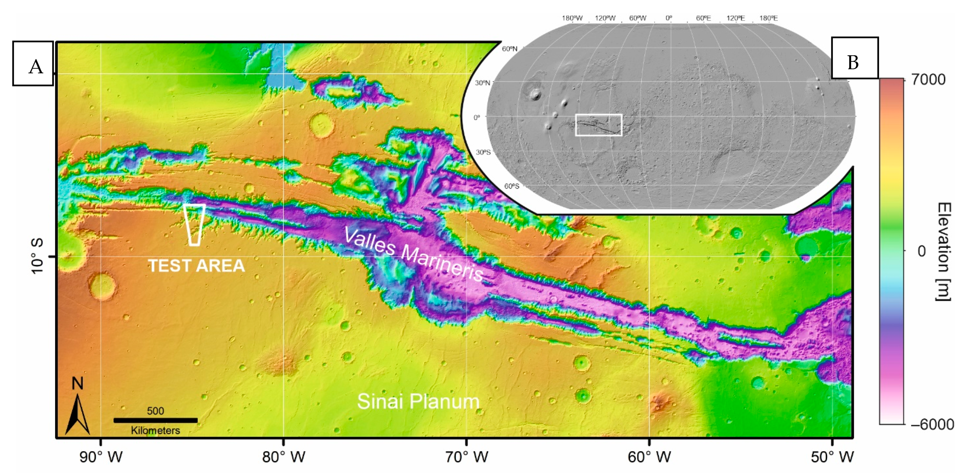
The method was tested in Valles Marineris (Figure 3). Most slopes are below 30°. Due to DTM resolution, steep cliffs are commonly reduced to lower slopes by averaging with neighboring slopes. The value of the steepest slope measured on the HRSC DTM is 57°.
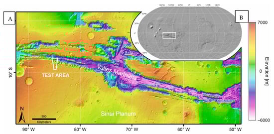
Figure 3.
Elevation map of the Valles Marineris region derived from the MEX HRSC Blended DEM Global 200m_v2 (A) with the location of the testing area on the MOLA shaded relief basemap adapted from [41] (B).
We evaluated our approach (Section 4.2) by comparing the ATIc values of three flat areas uniformly covered by a dune field with thermal inertia values from [2] and modelled values for dunes on Mars proposed by [42] and refined by [43].
3.1. Albedo
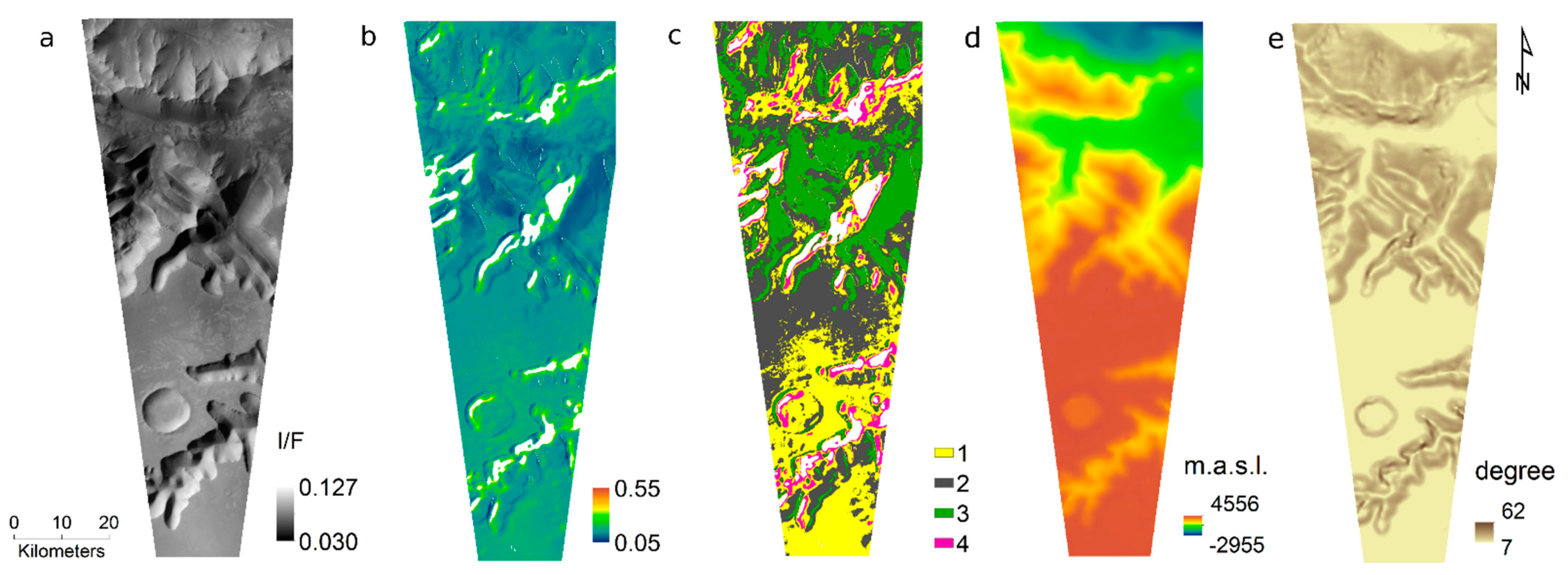
Albedo is calculated from the two mosaicked CTX images (Figure 4a). Topography-corrected albedo is calculated using Equation (7) and is in the range 0.05–0.55 (Figure 4b). HRSC DTM (Figure 4d) and slope (Figure 4e) maps show the topography and slopes distribution of the study area. Albedo arithmetic mean is 0.15. Four albedo classes are determined using unsupervised classification (Figure 4c, Table 1). Bell et al. (2008, their Table 2) linked albedo values with grain sizes. According to their classification, class 1 (0.17) mostly overlaps with fine representing dunes, class 2 with coarser sand or rocks (0.14), class 3 with dominant rock exposures—volcanic rocks and boulders (0.11), and class 4 with terrains dominated by sand and dust-sized particles (0.25) [44].
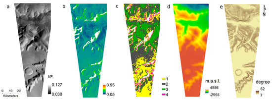
Figure 4.
(a) CTX visible light image mosaic of the test area (P01_001417_1718_XI_08S085W: t = 15.56 h, Ls = 135.5°, and P01_001351_1717_XI_08S084W: t = 15.55 h, Ls = 133.0°); (b) albedo map derived from CTX data, showing the albedo values corrected against topographic slope and aspect; (c) classes generated by unsupervised classification using the isodata algorithm [45] in IDRISI Selva [46]; the white zones in (b,c), which cover 6.2% of the image, are excluded from calculations due to incidence angle >79° or full shade; (d) Mars Express High-Resolution Stereo Camera (HRSC) digital terrain model (DTM) of the study area (in meters above sea level); (e) slope inclination map (in degrees) of the study area. Average albedo for each class is listed in Table 1. Coordinates of the top-left corner of the displayed area: 85°15′58.267″W, 7°8′57.982″S.

Table 2.
Selected characteristics of the THEMIS day and nighttime images used in the high-resolution apparent thermal inertia map calculation.
3.2. Surface Temperature
For remote observation of thermal inertia, measurements of day and night surface temperatures are required [27]. The maximum ∆T of any material is inversely proportional to thermal inertia. To calculate the thermal inertia of any material we have to know the maximum ∆T describing it. As Price [27] states, smaller values of thermal inertia P lead to greater day–night temperature contrast. Similarly, the effect of a smaller variation of flux to the atmosphere resulting from a given change of surface temperature (smaller) yields a larger day–night surface temperature contrast. Interpretation of the remotely sensed thermal inertia thus requires a proper portion of energy.
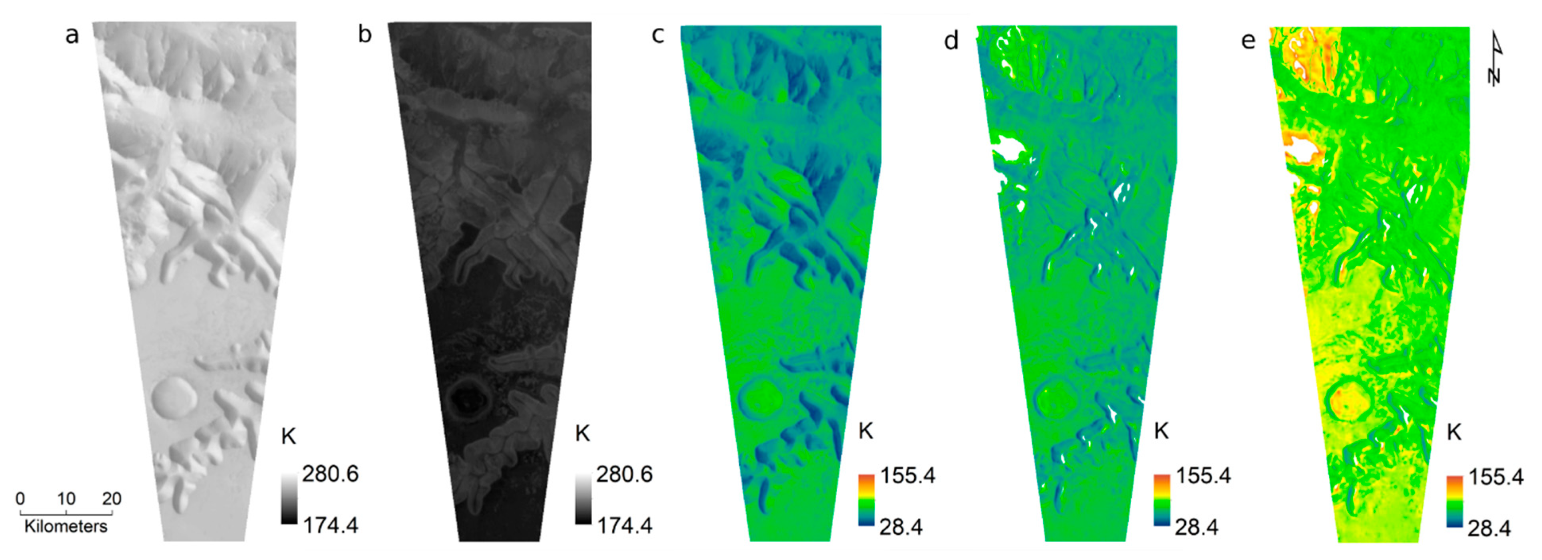
The study area is covered by a mosaic of two THEMIS daytime/nighttime image pairs (Figure 5a,b) from which diurnal temperature difference ΔT is calculated (Table 2). ∆T is the maximum surface temperature variation, usually calculated on a daily basis [47]. The THEMIS images are taken at full resolution (minimum and maximum “summing” parameters set to 1), and their image rating value (a subjective image quality assessment in the range 1–7) is 4 and 7, respectively. Due to discrete temperature measurements, the daily maximum temperature (and consequently daily temperature amplitude) needs to be estimated from submaximal temperature. Based on the MARSTHERM model, the maximum surface temperature falls typically at ~13:00, but all the daytime THEMIS images covering the study area in Valles Marineris are taken between 14:25 and 19:18. The selected set of images is therefore a trade-off between image rating, which needs to be as high as possible, and acquisition time, which needs to be as early as possible.

Figure 5.
(a) Daytime LST map; (b) nighttime map; (c) difference between daytime and nighttime LST; (d) difference between daytime and nighttime LST after correction following Equation (8); (e) difference between daytime and nighttime LST after correction following Equation (8) shifted to the real minimum and maximum of temperature (see second paragraph in Section 3.2). Images are IDs are provided in Table 2. The true temperature ranges are 229.5–280.6 K (a), 174.4–211.3 K (b), 28.4–82.0 K (c), 32.8–105.7 K (d), and 46.2–155.4 K (e). The white zones in (d,e) are excluded from calculations due to incidence angle > 79° or full shade.
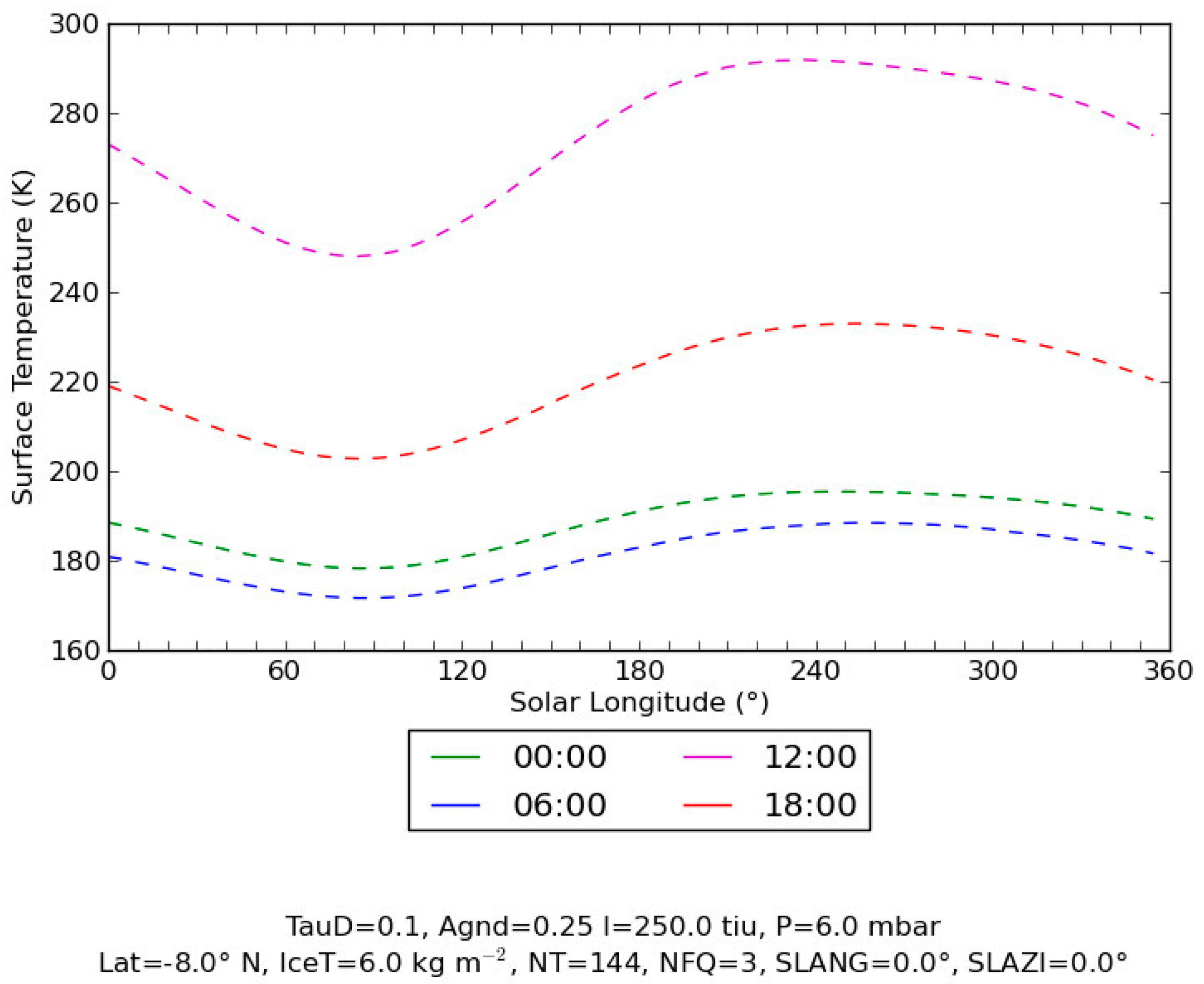
Equation (8) accounts for ΔT correction—derived from Supplementary File S2 (Part B) and explained in Equation (8). td in the equation stands for the time of the daytime image acquisition. The equation allows calculating the cumulative incidence radiation on an inclined surface for a given time interval (ΔT) accounting not only for solar geometry but also for slope inclination and orientation. Next, as the selected daytime THEMIS images used in our approach were taken at ~16:00 (Table 2), which deviates from the maximum temperature at 13:00 (Figure 6), we are counting a ratio of (T16:xx−Tmin)/(Tmax − T4:00) and divided our ∆T by the calculated ratio.
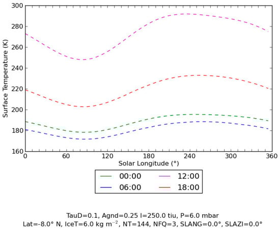
Figure 6.
Seasonal variability of surface temperature during a martian year at 8° S at 00:00 LST, 06:00 LST, 12:00 LST and 18:00 LST using MARSTHERM. TauD is dust opacity, Agnd is ground albedo, I is thermal inertia, P is surface pressure, Lat is latitude, IceT is the semi-infinite amount of CO2 ice with respect to albedo and emissivity in the MARSTHERM physical modelling scheme, NT is ground time step per day, with 10 min steps, NFQ is the number of ground time steps per atmospheric time step, SLANG is surface slope inclination, SLAZI is surface slope aspect.
For nighttime THEMIS images, we assume (in Equation (8)) that the Sun rises at 04:00, which is associated with a small error. For instance, sunrise at 05:00 LST or 07:00 would generate a temperature error of ~1 K or ~3 K, respectively. After topography correction, biased ΔT values for slopes are modified, whereas the ΔT values for flat areas remain unchanged. The real surface is mathematically transformed to a virtual flat surface in which ATIc does not depend on the topography (Figure 5c,d).
All the images represent the same season of the year—Southern Summer (270° to 360°/0°). The difference between the average Ls of the nighttime images and the average Ls of the daytime THEMIS images in the study area equals 4° (Table 2). According to Figure 6, the surface temperature at the same location will change with Ls. The seasonal variability of surface temperature curves in Figure 6 is derived for the 8° S latitude (location of the study area). This can cause an error of up to ~2 K between the assumed and true nighttime temperature, as it varies seasonally (see the 6:00 curve in Figure 6). For two daytime images with Ls = 319.1° and 271.2°, the temperature change in the study area is close to 5 K (4.65 K) at 18:00 (Figure 6). The temperature change is probably even lower (close to 4 K) as the images were taken earlier, at 16:16 and 16:73.
Dust opacity is estimated to be 0.22 in the study area (value for the pixel covering our study area). This number is extracted from the averaged maps of column dust optical depth (CDOD) at 9.3 µm normalised to the reference pressure of 610 Pa for MY (Mars years) 24, 25, and 26, using the gridded CDOD values from [35] with a spatial resolution of 6° × 3° (longitude x latitude) during the high dust loading season (Ls < 10° and Ls > 140°). Observations are from the TES and THEMIS images. We have also filtered the data from [35] by keeping only grid points for which the recorded time window TW = 1 sol, and the grid point reliability cdodrel >5 [35].
3.3. Apparent Thermal Inertia
Figure 7 shows the ATIc map (Figure 7a), and how it compares with [2] thermal inertia map (Figure 7b), hereafter called TI map. The difference between the ATIc and TI maps is in general small (Figure 7).
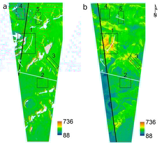
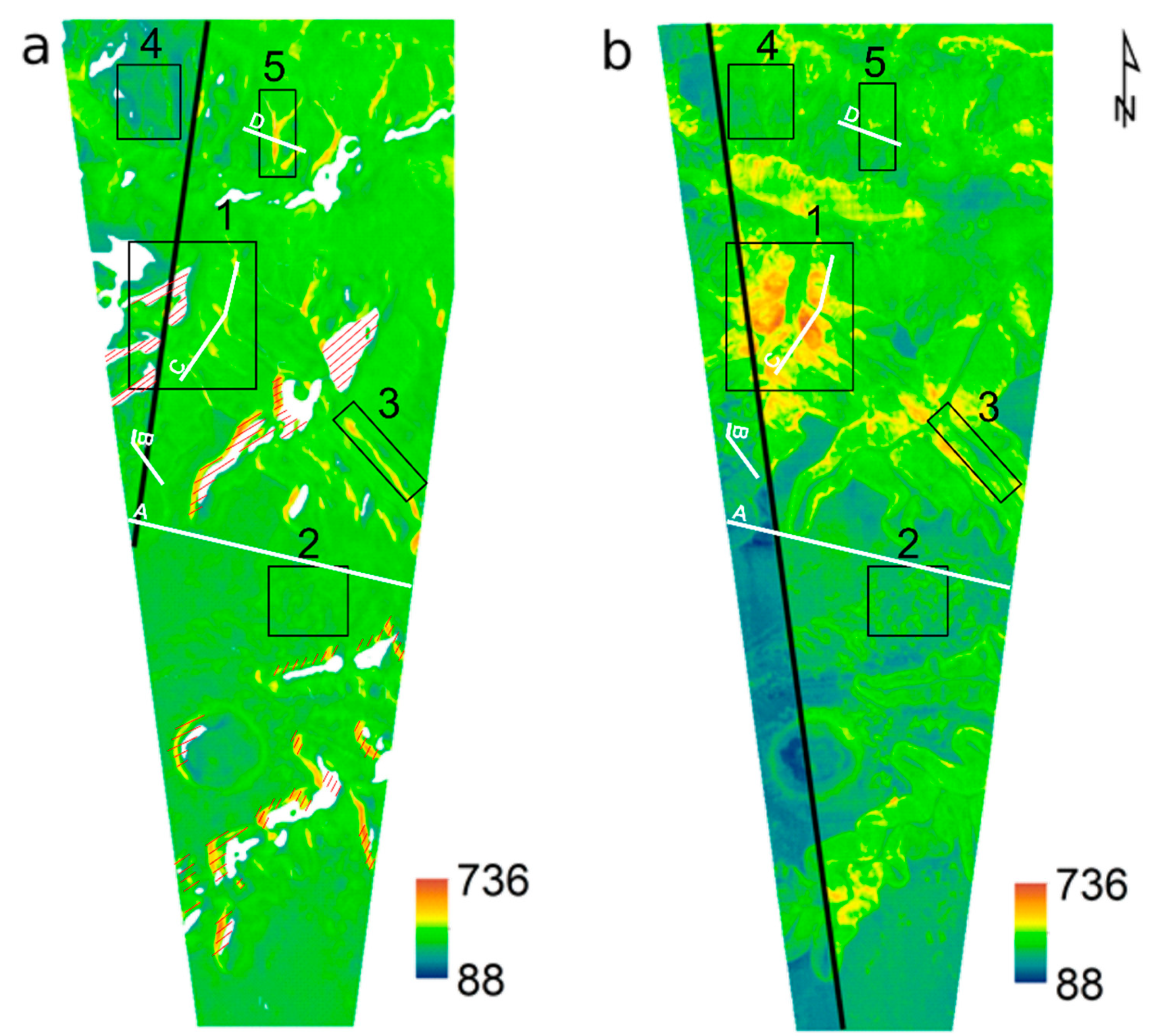
Figure 7.
(a) ATIc map (J m−2 K−1s−1/2); (b) thermal inertia (TI) map based on the thermal inertia mosaic of [2] released in 2014 (J m−2 K−1s−1/2). The thermal inertia scale in (a,b) has been unified for easier comparison; the true ranges are 157–729 for (a) and 88–736 for (b). The white zones in (a,b) are excluded from calculations due to incidence angle > 79° or full shade, which reduces the energy input on the slope. The thick black lines in (a,b) indicate boundaries between individual THEMIS images. The red-hatched zones in (a) receive high amount of reflected radiation (IR) (see Section 5.2 Model Limitations). Areas 1–5 are discussed in Section 4.1.
4. Analysis of Results
4.1. Overview
The boundary between THEMIS images outlines (“stamps”) is almost invisible after topographic image correction (Figure 7a, black line) and the two stamps represent the same range of values. It is a measure of the efficiency of the method in extracting thermophysical parameters from image-related parameters. In contrast, such a boundary is visible in the TI map. The differences in thermal inertia values between the two stamps exceed the limits of the thermal inertia measurements errors (Figure 7b, black line; see Section 2.6).
To correct ΔT against topography, the following steps need to be carried out (described in detail in Supplementary File S1 point IV–VI): (1) slopes and aspects calculation from DTM (in degrees), using, for example, HRSC/MEx (High-Resolution Stereo Camera onboard Mars Express orbiter); (2) calculation of the equation for cos(i) presented in Equation (7) in Supplementary File S2 (adapted to GIS in Supplementary File S1) by copy and paste to any Raster/Grid calculator tool in the selected GIS software; (3) finding the summed up value for the flat areas (F) typically represented by the mode; (4) application of the following Equation (11):
where ΔTc is corrected ΔT, F is the sum of all intervals (described in point V.2 in Supplementary File S1) and F0 is the F value for flat areas.
In addition, Figure 7 shows that the thermal inertia values using ATIc and TI in the study area are comparable in range (100–750), however, some significant differences exist. Moreover, the TI map has more colour gradations than the ATIc map due to topography artefacts and not due to the actual lithological as can be observed in several detailed examples (see Section 4.2).
The high thermal inertia located on the TI map (Figure 7—area 1) is the major difference. High thermal inertia is expected to correspond to abundant rocky outcrops. Geologic investigation of this area based on the available CTX and HiRISE images shows that this is not the case, and this high thermal inertia area is probably an artefact due to the absence of considering slopes on the TI map.
The top of Sinai Planum has dominantly low ATIc (<350, area 2), with convoluted patterns showing an ATIc of 350–370 related to eroded outcrops of layered deposits. These are known from other places in plateau areas around Valles Marineris [48] and are likely made of volcanic ash [2].
The lowest values (~250, area 3), are dominantly in the channel beds of Louros Valles and gullies of the Ius Chasma spur-and-gully slopes (e.g., [49]), and seem to correspond to dunes.
Most of the Louros Valles and Ius Chasma slopes (area 4) have ATIc values up to ~400, but locally even >700. The <400 values may correspond to debris flows or other flow types showing detrital accumulation of rocky material transported by gravity processes.
Significant differences between TI and ATI are observed in area 5. Here, ridge crests representing hard rocks exposures are more clearly visible on the ATIc with values ranging from 400–750 in contrast to lower values on the TI map. Geomorphological, e.g., [50], and petrological studies, e.g., [51], indicate these are volcanic outcrops, which is consistent with their relatively high values. Although these values are still 3−5 times lower than the thermal inertia values of fresh basalt [52], this is probably caused by weathering and partial regolithization of original basalts. Similar olivine-rich weathered basalt in easternmost Valles Marineris have also been found to have thermal inertia of 400–600 [20] (e.g., Area 5).
4.2. Method Validation
Comparing results for dune fields within ATIc and TI maps is a useful approach due to the existence of detailed studies on the role of grain size on thermal inertia under Martian pressure conditions [42,43,53]. Grain size is estimated based on terrestrial data by [43]—Table 3. Dune fields frequently occupy flat surfaces on Mars. ATIc for sands and other grain types are presented in Table 3 and calculated using Equation (1). Thermal conductivity (k) depends on pressure and grain size, and for a pressure of 613 Pa is:
where d is grain size diameter in µm [43].
K = 0.00375d0.467
Table 3.
Apparent thermal inertia of grains on Mars as a function of grain size. Grain classification and grain size ranges are from [54].
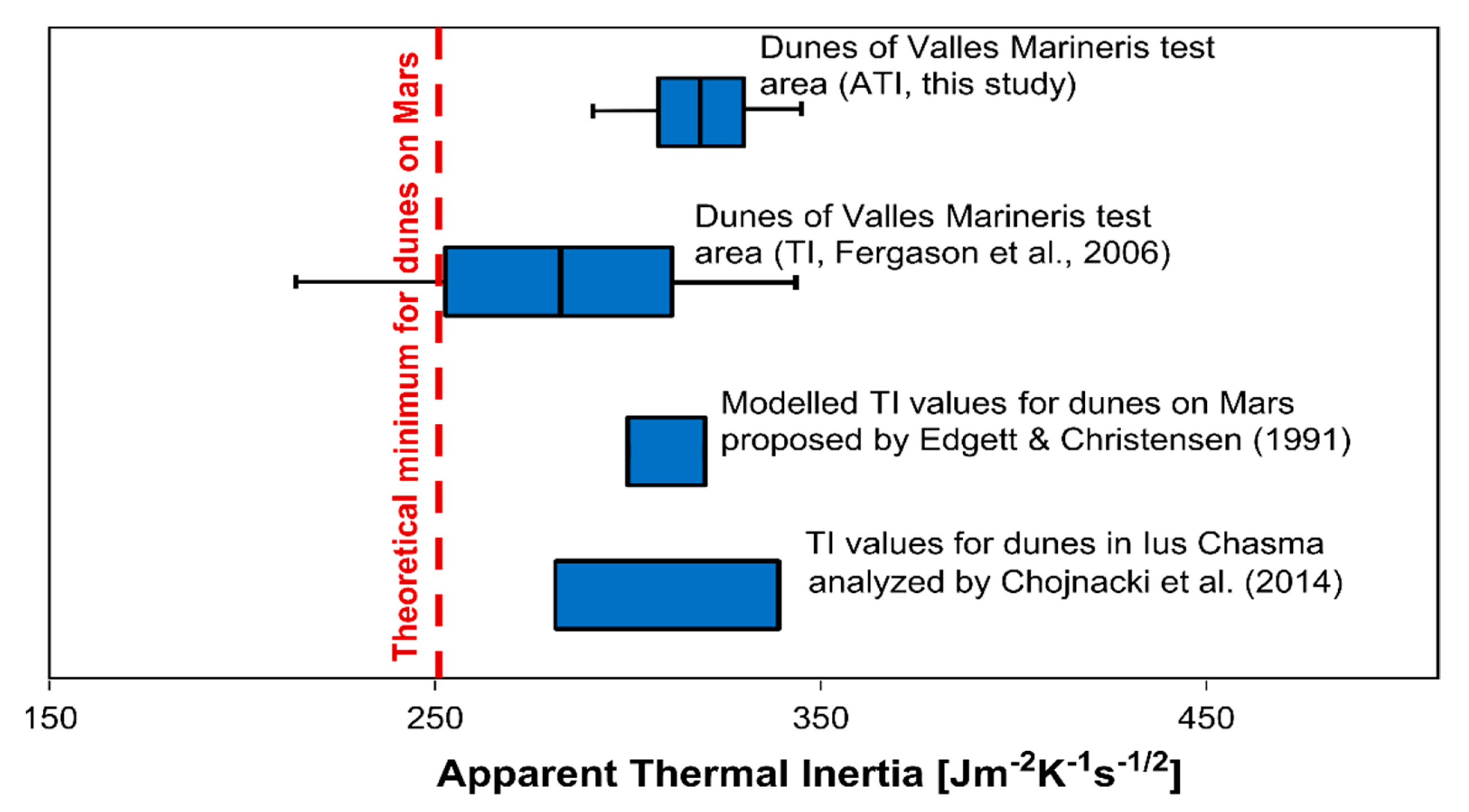
For three flat areas uniformly covered by a dune field (Figure 8), ATIc is very similar and they agree with the modelled values for dunes on Mars proposed by [42] and refined by [43]. The average ATIc, and TI of the three dune fields overlap with the average ATIc of 320, and 282 for TI (Figure 9). The average thermal inertia for the three dune fields is 235, 291, and 314 (TI) and 310, 319, and 334 (ATIc) respectively. For each of these maps, the largest discrepancies (235 vs. 291/314—TI; 310/319 vs. 334—ATIc) are found when measured on different THEMIS image pairs (image boundaries are reported in Figure 7a,b). The theoretical minimum in Figure 9 is calculated considering the empirical relationship between thermal conductivity and grain size derived by [43], assuming a specific heat of 850 J·kg−1·K−1 and a bulk density of 1650.0 kg·m−3, as proposed by [52].
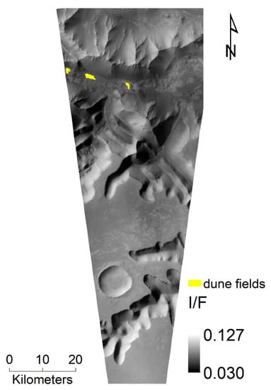
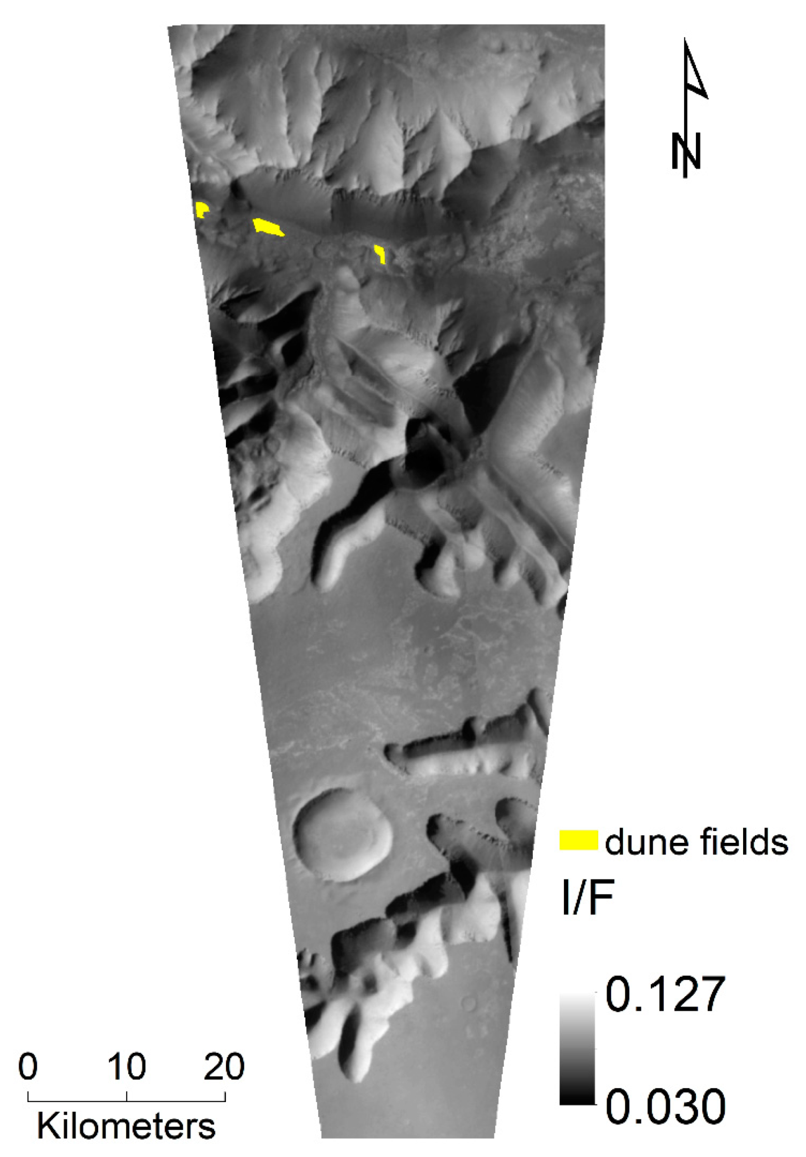
Figure 8.
MRO/CTX visible light image mosaic of the study area and the dune fields tested for ATIc evaluation.
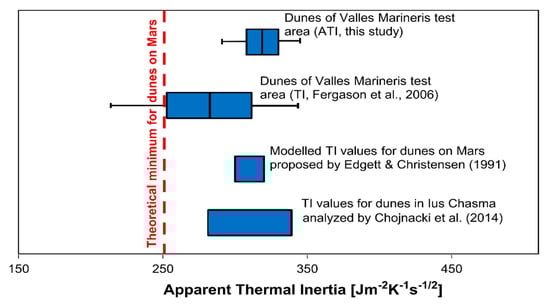
Figure 9.
Thermal inertia for dunes according to ATIc calculation and other methods. Whiskers represent the total range of values for the dune fields in Figure 8, and the blue boxes span from the arithmetic mean to ±1 standard deviation. The value of the red line (251) is calculated from the theoretical minimum dune sand grain size of 215 µm in Martian conditions [42] and empirical relationship between thermal conductivity and grain size derived by [43] assuming a specific heat of 850 J·kg−1/K−1 and a bulk density of 1650.0 kg·m−3 [52]. Similarly, the modelled TI values are derived assuming typical 470–600 µm grain size provided by [42].
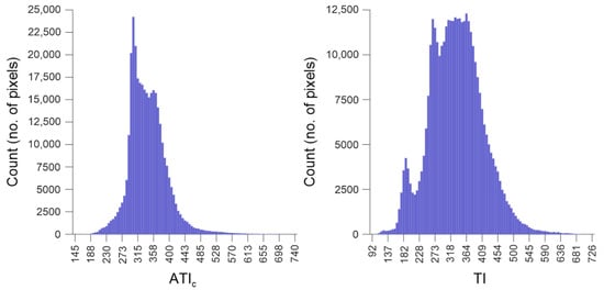
Both the ATIc and TI maps indicate a globally sandy surface and shows a multimodal distribution, with two modes on the ATIc map, and three modes on the TI map (Figure 10). The two modes observed on the ATIc and TI maps represent fine (~250) and coarse (~350) sand. The “finest fraction” mode on the TI map (~185) is an artefact resulting from the THEMIS mosaic boundary, and in fact, represents the area to the left of the black line shown in Figure 7b. Apart from these differences, ATIc and TI seem to give similar results on flat, sandy areas.
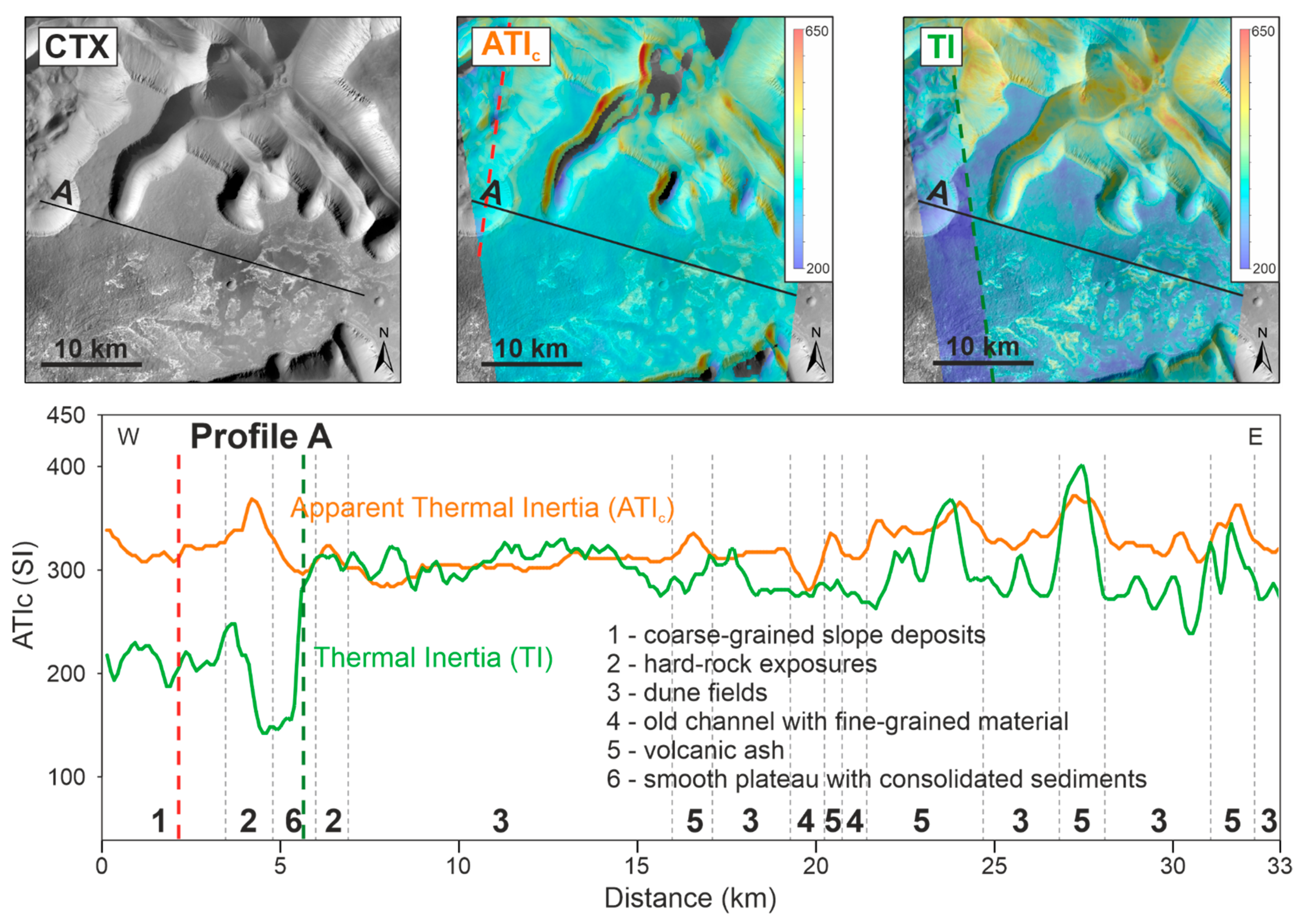
This is particularly well visible on the regional profile A (Figure 7) presented in Figure 11. Here, dune fields show mostly the same value of ~310 but the range of TI values within the profile is broader (~90) than for ATIc (~50) even within the same CTX image. This may result from some artificial linear boundaries perpendicular to the profile such as the one around 15 km of the profile visible on the TI image. Even more pronounced differences are visible between the CTX images (green boundary for TI and orange boundary for ATIc on Figure 11). On the TI-CTX boundary, there is a jump of >100 tiu within the consolidated sediments of the smooth plateau. A similar jump (within the coarse-grained slope deposits) on the ATIc-CTX boundary seems to be <20.

Figure 11.
Regional profile across a flat part of the study area. Thermal inertia (TI) results of Fergason et al. [2] are compared to our ATI results and geomorphological interpretation of the surface. Note the CTX image boundaries in both methods and their effects on the obtained results.
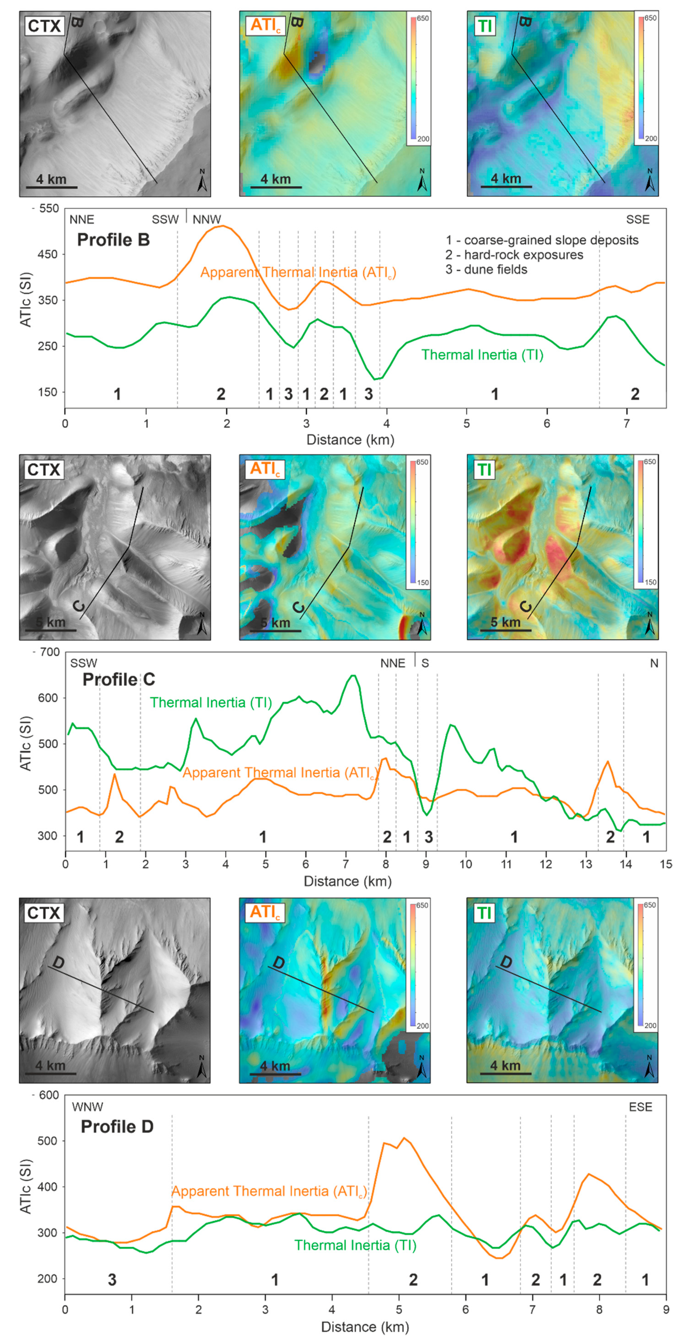
However, within the same image, both methods seem to be relatively well distinguished between various geological terrains. For example, volcanic ashes show systematically higher values than dune fields, and hard-rock exposures systematically higher values than coarse-grained slope deposits (Profile A in Figure 11 and Profile B in Figure 12). Yet, there are also exceptions especially for fine-scale features such as two in Profile D (Figure 12), where the TI method seems to be insensitive for hard-rock exposures well visible on the CTX and ATIc images. On Profile C in Figure 12, the TI profile shows an excellent sensitivity for little dune field in the valley but values for coarse-grained slope deposits on steep slopes seem to be exaggerated. This may be related to method deficiency on the slopes >10° mentioned by Fergason et al. [2]. The ATIc profile D seems to yield more consistent results for these coarse-grained slope deposits, less affected by non-geological factors such as slope inclination and orientation.
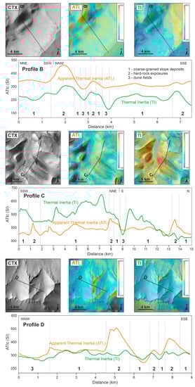
Figure 12.
High-resolution profiles across various slopes in the study area. Thermal inertia (TI) results of Fergason et al. [2] are compared to our ATI results and geomorphological interpretation of the surface.
5. Discussion
5.1. Model Strengths and Applicability
A new method for high-resolution apparent thermal inertia mapping on Mars is presented. Our method is based on the algorithm using a set of publicly available data that is temperature, albedo, solar geometry, visible dust opacity, and a digital elevation model. This approach could hopefully serve a broader community of researchers interested in the thermal properties of rocks on Mars. We took into account local topography characteristics (slope inclination and aspect) for different insolation rates on inclined surfaces, which heavily affects albedo and temperature. As our approach has been tested in a challenging area of Valles Marineris, we think that thermal mapping using THEMIS is possible in any area of Mars, independently of its local topography. The use of the ATIc method for fine-scale geologic studies may be advantageous.
Specifically, we have tested our method in the following aspects: (1) layered deposits/volcanic ash: Figure 7—area 2; (2) Martian sands/dunes occurrence (including grain size distinction)—area 3; (3) gravity slopes—area 4; (4) rocky outcrops (e.g., ridge crest)— area 5. ATIc values remain the same in opposite slopes where they expose the same rock (the effect of the time of the day was removed). On the other hand, for flat areas (dunes fields, layered deposits), ATIc and TI values remain similar, which sup-ports the validity of our method on flat areas.
The applicability of ATIc to geological studies is thus broad. Firstly, ATIc may help to distinguish magmatic volcanic cones from mud volcanoes [55] and can be even applied to distinguish between effusive and explosive magmatic volcanism by identification of pyroclastic deposits in volcanic areas. According to Brož et al. [56], Martian explosive volcanoes such as scoria cones are expected on Mars as on Earth, they commonly occur on the terrestrial basaltic volcanoes and associated volcanic plains. These are small edifices difficult to recognise. Hauber et al. [57] pointed out that grain size analysis can be helpful in their identifications as they consist of relatively fine tephra particles or some other fragmented material. Although based on numerical modelling of [58,59], the ejected particles forming Martian scoria cones should be ~20 times finer than is typical on Earth, this is still corresponding to a mean particle size of ~2 mm on Mars, so significantly more than typical Aeolian deposits such as dunes.
Secondly, ATIc may be useful to determine grain size variation related to changes in depositional environments (e.g., in the Murray Formation in the Gale Crater [60]) as well as grain size data for eolian ripples and dunes estimations of wind and climatic conditions on Mars [61].
Thirdly, Di Pietro et al. [62] made a detailed thermal inertia map using differential apparent thermal inertia technique on a selected portion of the studied area (thumbprint terrains in Acidalia Planitia) to give information on the particle sizes and more generally, thermophysical properties of the soil. After analysing all the datasets (differential apparent thermal inertia technique, Context Camera, High-Resolution Imaging Science Experiment images, and topographic profiles based on Mars Orbiter Laser Al-timeter) they supported the tsunami-driven mud-volcanoes hypothesis in the study area.
5.2. Model Limitations
Although the algorithm presented here works well in most configurations of orientation and slope, three limitations are identified. The first is related to the very steep slopes in the shade at the time the CTX image is taken, or before the THEMIS IR day image is taken (white zones on Figure 7a). The incidence angle on these slopes is so high that it generates large errors in the ATIc calculation.
The second limitation is met in areas where the horizon reduces the total energy input due to shading. Shading may especially occur at mid-slope in impact crater rims or other concave slopes. We filtered out all the instances where shading happens (<0.1% of the studied area) using the Analytical Hillshading tool in SAGA GIS, as explained in the tutorial in Supplementary File S1, to ensure that we avoid erroneous ATI values in these areas.
The third limitation is related to the area of a high amount of reflected radiation (IR). Our approach does not account for the radiation potentially reflected from the neighbouring surface. Assuming an infinite flat surface in front of an inclined surface of slope angle s, following [63,64,65], the ratio (R) of this radiation, with respect to the total incident radiation (F), can be calculated as:
R = 0.5A (1 − cos(s))
In the case of a valley, the radiation reflected on this inclined surface by the opposite slope, of angle s*, Equation (13) becomes [66]:
R = 0.5A (1 − cos(s + s*))
To calculate this percentage (Figure 13) more accurately, we need to consider that the two facing slopes receive uneven amounts of primary radiation due to their different orientation relative to the sun, and the slope that receives the least primary radiation receives the most reflected radiation from the other slope. In order to account for this effect, Equation (14) should be modified to:
where F(s) is the total radiation for the observed slope, and F(s*) is the total radiation for the opposite slope. Equation (15) implies that although the proportion of reflected radiation with respect to the total radiation is typically 1–5%, it could be infinitely higher if F(s) approaches zero.

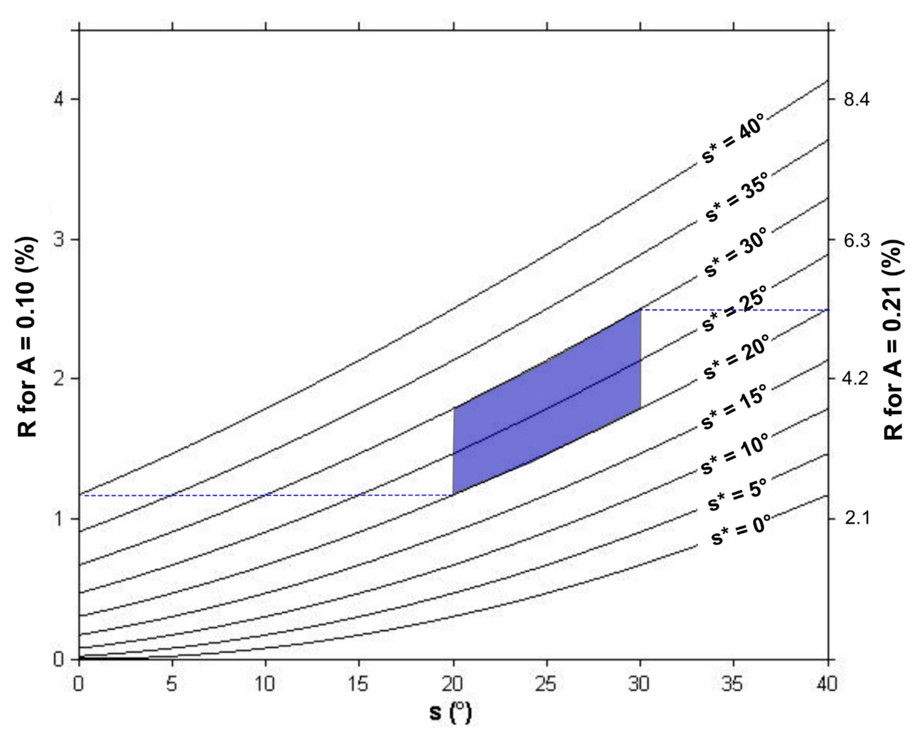
Figure 13.
Percentage (R) of the reflected radiation (IR) with respect to the total radiation calculated with Equation (14) as a function of the observed slope (s), opposite slope (s*), and albedo (A). The blue field indicates the expected error range (1.2 to 5.3%, dashed lines) for the valleys in the study area, where typical slopes are 20–30° and albedo is 0.10–0.21.
This is the case for the west-facing valley slopes in the early morning, and the east-facing valley slopes in the late afternoon. This transitory behavior yields little impact on temperature correction due to the integration over a broader time interval (Equation (7)). For the albedo correction, though, the effect may become significant in special cases. In the case studied in Section 4, where the CTX images were taken in the afternoon, east-facing slopes receive relatively higher amounts of reflected radiation (IR). Consequently, the total radiation (F) is overestimated; for example, by up to 60% for NE-SW oriented valleys with 30°-steep slopes in Figure 7a, assuming a typical albedo of 0.21. The calculated albedo would then be 37.5% too low, and the calculated ATIc, 10% too high. This is likely the reason why anomalously high ATIc values are sometimes obtained for the east-facing slopes (the red-hatched zones in Figure 7a) compared to the west-facing slopes, in ~1% of the studied area. For most slopes with inclinations of 10–30° in this area, this effect is almost negligible (<5%), and the slopes 10–30° steep are still beyond the threshold of 10° reported in the validation of [2] model. This issue is expected to be infrequent outside the Valles Marineris area because it requires a very narrow valley with steep to medium slopes.
The fourth limitation is also related to sloped surfaces, which irradiate toward a solid angle <2π sr. This limitation is also important, particularly inside valleys and canyons. The effect of this is that sloped surfaces remain warmer longer than similar but flat surfaces, which may affect both night (dawn) and day (afternoon) temperature and thus also ATI as this has not been accounted for in our correction.
6. Conclusions
The TI approach used so far on Mars is adapted to the observation scale where slopes can be neglected. In contrast, the proposed ATIc technique, while being consistent with TI at such scales, makes it possible to go into processes that are slope-dependent, generally smaller-scale. Importantly, the presented method is based on the algorithm using a set of publicly available data comprising temperature, albedo, solar geometry, visible dust opacity, and a digital elevation model.
The proposed technique should be especially useful for geomorphologists, but hopefully also for geologists working on rock composition, mechanical properties, and, more generally, geological processes on steep slopes. ATIc has a wide range of applications discussed in Section 5, especially in combination with other datasets. These include, for example, (1) providing an origin for thumbprint terrains and constrains for the geological evolution of Acidalia Planitia; (2) grain size analysis in the Martian explosive volcanoes identifications consisting of fine tephra particles or some other fragmented material; (3) grain size variations to track changes in depositional environments; (4) distinguishing volcano cones from mud volcanoes; (5) identification of layered deposits, volcanic ash, sands and dunes, gravity slopes and rocky outcrops.
Supplementary Materials
The following are available online at https://www.mdpi.com/article/10.3390/rs13183692/s1, Supplementary File S1, Supplementary File S2, Supplementary File S3.
Author Contributions
Conceptualization, M.C. and J.C.; methodology, M.C. and J.C.; software, M.C.; validation, M.C. and J.C.; formal analysis, M.C. and J.C.; investigation, M.C. and J.C.; resources, M.C., J.C. and B.P.; data curation, M.C., J.C. and B.P.; writing—original draft preparation, M.C. and J.C.; writing—review and editing, M.C. and J.C. and B.P.; visualization, M.C., J.C. and B.P. All authors have read and agreed to the published version of the manuscript.
Funding
This research was funded by the TEAM programme of the Foundation for Polish Science (projects TEAM/2011-7/9 and TEAM/2016-3/20), co-financed by the European Union within the framework of the European Regional Development Fund, and National Science Centre of Poland project OPUS19 no. 2020/37/B/ST10/01420. B. Pieterek is financially supported by the European Funds Smart Growth (PO WER) project no. POWR.03.02.00−00−I027/17 held by the Adam Mickiewicz University in Poznan.
Institutional Review Board Statement
Not applicable.
Informed Consent Statement
Not applicable.
Acknowledgments
The authors would like to thank Daniel Mège from Space Research Centre of Polish Academy of Sciences, Paulina Wolkenberg from Istituto di Astrofisica e Planetologia Spaziali, Andrew Ryan from Arizona State University, Jonathon Hill from Mars Space Flight Facility, and Joshua Bandfield from Space Science Institute for their valuable comments during writing this paper. This work was supported by the TEAM programme of the Foundation for Polish Science (projects TEAM/2011-7/9 and TEAM/2016-3/20), co-financed by the European Union within the framework of the European Regional Development Fund, as well as National Science Centre of Poland project OPUS19 no. 2020/37/B/ST10/01420. B. Pieterek is financially supported by the European Funds Smart Growth (PO WER) project no. POWR.03.02.00−00−I027/17 held by the Adam Mickiewicz University in Poznan. We thank editor Jerry Xiong, academic editors, and three anonymous reviewers for their thorough and insightful comments.
Conflicts of Interest
The authors declare no conflict of interest.
References
- Piqueux, S.; Christensen, P.R. Temperature-dependent thermal inertia of homogeneous Martian regolith. J. Geophys. Res. Planets 2011, 116. [Google Scholar] [CrossRef]
- Fergason, R.L.; Christensen, P.R.; Kieffer, H.H. High-resolution thermal inertia derived from the Thermal Emission Imaging System (THEMIS): Thermal model and applications. J. Geophys. Res. Planets 2006, 111. [Google Scholar] [CrossRef]
- Neugebauer, G.; Münch, G.; Kieffer, H.; Chase Jr, S.C.; Miner, E. Mariner 1969 infrared radiometer results: Temperatures and thermal properties of the Martian surface. Astron. J. 1971, 76, 719–749. [Google Scholar] [CrossRef] [Green Version]
- Morrison, D.; Sagan, C.; Pollack, J.B. Martian temperatures and thermal properties. Icarus 1969, 11, 36–45. [Google Scholar] [CrossRef]
- Kieffer, H.H.; Chase, S.C., Jr.; Miner, E.; Münch, G.; Neugebauer, G. Preliminary report on infrared radiometric measurements from the Mariner 9 spacecraft. J. Geophys. Res. 1973, 78, 4291–4312. [Google Scholar] [CrossRef] [Green Version]
- Kieffer, H.H.; Martin, T.Z.; Peterfreund, A.R.; Jakosky, B.M.; Miner, E.D.; Palluconi, F.D. Thermal and albedo mapping of Mars during the Viking primary mission. J. Geophys. Res. 1977, 82, 4249–4291. [Google Scholar] [CrossRef]
- Kieffer, H.H. Thermal model for analysis of Mars infrared mapping. J. Geophys. Res. Planets 2013, 118, 451–470. [Google Scholar] [CrossRef]
- Vdovin, V.V.; Zhegulev, V.S.; Ksanfomaliti, L.V.; Moroz, V.I.; Petrova, E.V. Some characteristics of the soil in the equatorial zone of Mars according to the thermal radiometry data from Mars 5. Cosm. Res. 1981, 18, 609–622. [Google Scholar]
- Palluconi, F.D.; Kieffer, H.H. Thermal inertia mapping of Mars from 60 S to 60 N. Icarus 1981, 45, 415–426. [Google Scholar] [CrossRef]
- Haberle, R.M.; Jakosky, B.M. Atmospheric effects on the remote determination of thermal inertia on Mars. Icarus 1991, 90, 187–204. [Google Scholar] [CrossRef]
- Christensen, P.; Moore, H.J. The Martian surface layer. In Mars; Kieffer, H.H., Ed.; University of Arizona Press: Tucson, AZ, USA, 1992; pp. 686–729. [Google Scholar]
- Dollfus, A.; Deschamps, M.; Zimbelman, J.R. Soil texture and granulometry at the surface of Mars. J. Geophys. Res. Planets 1993, 98, 3413–3429. [Google Scholar] [CrossRef] [Green Version]
- Zent, A.P.; Haberle, R.M.; Houben, H.C.; Jakosky, B.M. A coupled subsurface-boundary layer model of water on Mars. J. Geophys. Res. Planets 1993, 98, 3319–3337. [Google Scholar] [CrossRef]
- Jakosky, B.M.; Mellon, M.T.; Kieffer, H.H.; Christensen, P.R.; Varnes, E.S.; Lee, S.W. The thermal inertia of Mars from the Mars global surveyor thermal emission spectrometer. J. Geophys. Res. Planets 2000, 105, 9643–9652. [Google Scholar] [CrossRef]
- Mellon, M.T.; Jakosky, B.M.; Kieffer, H.H.; Christensen, P.R. High-resolution thermal inertia mapping from the Mars global surveyor thermal emission spectrometer. Icarus 2000, 148, 437–455. [Google Scholar] [CrossRef]
- Putzig, N.E.; Mellon, M.T.; Kretke, K.A.; Arvidson, R.E. Global thermal inertia and surface properties of Mars from the MGS mapping mission. Icarus 2005, 173, 325–341. [Google Scholar] [CrossRef]
- Price, J.C. On the analysis of thermal infrared imagery: The limited utility of apparent thermal inertia. Remote Sens. Environ. 1985, 18, 59–73. [Google Scholar] [CrossRef]
- Xue, Y.; Cracknell, A.P. Advanced thermal inertia modelling. Remote Sens. 1995, 16, 431–446. [Google Scholar] [CrossRef]
- Cracknell, A.P.; Xue, Y. Thermal inertia determination from space—a tutorial review. Int. J. Remote Sens. 1996, 17, 431–461. [Google Scholar] [CrossRef]
- Edwards, C.S.; Piqueux, S. The water content of recurring slope lineae on Mars. Geophys. Res. Lett. 2016, 43, 8912–8919. [Google Scholar] [CrossRef]
- Hamilton, V.E.; Vasavada, A.R.; Sebastián, E.; de la Torre Juárez, M.; Ramos, M.; Armiens, C.; Arvidson, R.E.; Carrasco, I.; Christensen, P.R.; De Pablo, M.A. Observations and preliminary science results from the first 100 sols of MSL Rover Environmental Monitoring Station ground temperature sensor measurements at Gale Crater. J. Geophys. Res. Planets 2014, 119, 745–770. [Google Scholar] [CrossRef] [Green Version]
- Sabol, D.E.; Gillespie, A.R.; McDonald, E.; Danillina, I. Differential thermal inertia of geological surfaces. In Proceedings of the 2nd Annual International Symposium of Recent Advances in Quantitative Remote Sensing, Torrent, Spain, 25–29 September 2006; pp. 25–29. [Google Scholar]
- Putzig, N.E.; Mellon, M.T. Apparent thermal inertia and the surface heterogeneity of Mars. Icarus 2007, 191, 68–94. [Google Scholar] [CrossRef]
- Scheidt, S.; Ramsey, M.; Lancaster, N. Determining soil moisture and sediment availability at White Sands Dune Field, New Mexico, from apparent thermal inertia data. J. Geophys. Res. Earth Surf. 2010, 115. [Google Scholar] [CrossRef]
- Kubiak, M.; Stach, A. The use of motor-glider in topoclimatic studies. Int. J. Appl. Earth Obs. Geoinf. 2014, 32, 186–198. [Google Scholar] [CrossRef]
- Kubiak, M.; Mège, D.; Gurgurewicz, J.; Ciazela, J. Thermal mapping of mountain slopes on Mars by application of a Differential Apparent Thermal Inertia technique. In Proceedings of the EGU General Assembly Conference, Vienna, Austria, 12–17 April 2015; p. 1030. [Google Scholar]
- Price, J.C. Thermal inertia mapping: A new view of the earth. J. Geophys. Res. 1977, 82, 2582–2590. [Google Scholar] [CrossRef]
- Kahle, A.B. Geologic Application of Thermal Inertia Imaging Using HCMM Data; National Aeronautics and Space Administration, Jet Propulsion Laboratory: Pasadena, CA, USA, 1981. [Google Scholar]
- Kahle, A.B. A simple thermal model of the Earth’s surface for geologic mapping by remote sensing. J. Geophys. Res. 1977, 82, 1673–1680. [Google Scholar] [CrossRef]
- Coakley, J.A., Jr. Reflectance and Albedo, Surface. In Encyclopedia of the Atmosphere; Holton, J.R., Curry, J.A., Eds.; Academic Press: Cambridge, MA, USA, 2002. [Google Scholar]
- Malin, M.C.; Bell, J.F.; Cantor, B.A.; Caplinger, M.A.; Calvin, W.M.; Clancy, R.T.; Edgett, K.S.; Edwards, L.; Haberle, R.M.; James, P.B. Context camera investigation on board the Mars Reconnaissance Orbiter. J. Geophys. Res. Planets 2007, 112. Available online: https://agupubs.onlinelibrary.wiley.com/doi/full/10.1029/2006JE002808 (accessed on 14 September 2021).
- Christensen, P.R.; Bandfield, J.L.; Hamilton, V.E.; Ruff, S.W.; Kieffer, H.H.; Titus, T.N.; Malin, M.C.; Morris, R.V.; Lane, M.D.; Clark, R.L.; et al. Mars Global Surveyor Thermal Emission Spectrometer experiment: Investigation description and surface science results. J. Geophys. Res. Planets 2001, 106, 23823–23871. [Google Scholar] [CrossRef]
- Bell, J.F.; Malin, M.C.; Caplinger, M.A.; Fahle, J.; Wolff, M.J.; Cantor, B.A.; James, P.B.; Ghaemi, T.; Posiolova, L.V.; Ravine, M.A.; et al. Calibration and Performance of the Mars Reconnaissance Orbiter Context Camera (CTX). Int. J. Mars Sci. Explor. 2013, 8, 1–14. [Google Scholar] [CrossRef]
- Becker, K.J.; Anderson, J.A.; Weller, L.A.; Becker, T.L. ISIS support for NASA mission instrument ground data processing systems. In Proceedings of the Lunar and Planetary Science Conference, The Woodlands, TX, USA, 18–22 March 2013; Volume 44, p. 2829. [Google Scholar]
- Montabone, L.; Forget, F.; Millour, E.; Wilson, R.J.; Lewis, S.R.; Cantor, B.; Kass, D.; Kleinböhl, A.; Lemmon, M.T.; Smith, M.D. Eight-year climatology of dust optical depth on Mars. Icarus 2015, 251, 65–95. [Google Scholar] [CrossRef] [Green Version]
- Montabone, L.; Cantor, B.; Forget, F.; Kass, D.; Kleinboehl, A.; Smith, M.D.; Wolff, M.J. On the Dustiest Locations on Mars from Observations. In Proceedings of the Sixth International Workshop on The Mars Atmosphere: Modelling and Observations, Granada, Spain, 17 January 2017; pp. 17–20. [Google Scholar]
- Forget, F.; Montabone, L. Atmospheric dust on Mars: A review. In Proceedings of the 47th International Conference on Environmental Systems, Charleston, SC, USA, 16–20 July 2017. [Google Scholar]
- Gwinner, K.; Scholten, F.; Spiegel, M.; Schmidt, R.; Giese, B.; Oberst, J.; Heipke, C.; Jaumann, R.; Neukum, G. Derivation and validation of high-resolution digital terrain models from Mars Express HRSC data. Photogramm. Eng. Remote Sens. 2009, 75, 1127–1142. [Google Scholar] [CrossRef] [Green Version]
- Zevenbergen, L.W.; Thorne, C.R. Quantitative analysis of land surface topography. Earth Surf. Process. Landf. 1987, 12, 47–56. [Google Scholar] [CrossRef]
- Heipke, C.; Oberst, J.; Albertz, J.; Attwenger, M.; Dorninger, P.; Dorrer, E.; Ewe, M.; Gehrke, S.; Gwinner, K.; Hirschmüller, H. Evaluating planetary digital terrain models—The HRSC DTM test. Planet. Space Sci. 2007, 55, 2173–2191. [Google Scholar] [CrossRef]
- Tanaka, K.L.; Skinner, J.A., Jr.; Dohm, J.M.; Irwin, R.P., III; Kolb, E.J.; Fortezzo, C.M.; Platz, T.; Michael, G.G.; Hare, T.M. Geologic map of Mars. Sci. -Investig. Map 2014. [Google Scholar] [CrossRef]
- Edgett, K.S.; Christensen, P.R. The particle size of Martian aeolian dunes. J. Geophys. Res. Planets 1991, 96, 22765–22776. [Google Scholar] [CrossRef]
- Presley, M.A.; Christensen, P.R. The effect of bulk density and particle size sorting on the thermal conductivity of particulate materials under Martian atmospheric pressures. J. Geophys. Res. Planets 1997, 102, 9221–9229. [Google Scholar] [CrossRef]
- Bell, J.F.; Rice, M.S.; Johnson, J.R.; Hare, T.M. Surface albedo observations at Gusev Crater and Meridiani Planum, Mars. J. Geophys. Res. E Planets 2008, 113, 1–13. [Google Scholar] [CrossRef] [Green Version]
- Ball, G.H.; Hall, D.J. ISODATA, A Novel Method of Data Analysis and Pattern Classification; Stanford Research Institute: Menlo Park, CA, USA, 1965. [Google Scholar]
- Eastman, J.R. IDRISI Selva; Clark Labs-Clark University: Worcester, MA, USA, 2012. [Google Scholar]
- Minacapilli, M.; Cammalleri, C.; Ciraolo, G.; D’Asaro, F.; Iovino, M.; Maltese, A. Thermal Inertia Modeling for Soil Surface Water Content Estimation: A Laboratory Experiment; Thermal Inertia Modeling for Soil Surface Water Content Estimation: A Laboratory Experiment. Soil Sci. Soc. Am. J. 2012, 76, 92–100. [Google Scholar] [CrossRef]
- Le Deit, L.; Bourgeois, O.; Mège, D.; Hauber, E.; Le Mouélic, S.; Massé, M.; Jaumann, R.; Bibring, J.-P. Morphology, stratigraphy, and mineralogical composition of a layered formation covering the plateaus around Valles Marineris, Mars: Implications for its geological history. Icarus 2010, 208, 684–703. [Google Scholar] [CrossRef]
- Lucchitta, B.K.; McEwen, A.S.; Clow, G.D.; Geissler, P.E.; Singer, R.B.; Schultz, R.A.; Squyres, S.W. Valles Marineris. In Mars; University of Arizona Press: Tuscon, AZ, USA, 1992; pp. 453–492. [Google Scholar]
- Beyer, R.A.; McEwen, A.S. Layering stratigraphy of eastern Coprates and northern Capri Chasmata, Mars. Icarus 2005, 179, 1–23. [Google Scholar] [CrossRef]
- Flahaut, J.; Quantin, C.; Clenet, H.; Allemand, P.; Mustard, J.F.; Thomas, P. Pristine Noachian crust and key geologic transitions in the lower walls of Valles Marineris: Insights into early igneous processes on Mars. Icarus 2012, 221, 420–435. [Google Scholar] [CrossRef]
- Mellon, M.T.; Fergason, R.L.; Putzig, N.E. The thermal inertia of the surface of Mars. Martian Surf.-Compos. Mineral. Phys. Prop. 2008, 399, 399–427. [Google Scholar] [CrossRef]
- Edgett, K.S.; Christensen, P.R. Mars aeolian sand: Regional variations among dark-hued crater floor features. J. Geophys. Res. Planets 1994, 99, 1997–2018. [Google Scholar] [CrossRef]
- Wentworth, C.K. A scale of grade and class terms for clastic sediments. J. Geol. 1922, 30, 377–392. [Google Scholar] [CrossRef]
- Leszek, C.; Natalia, Z.; Anita, Z.; Marta, C.; Witek Piotr, K.J. The mechanisms of formation of some small cones in Chryse Planitia on Mars. In Proceedings of the EGU General Assembly 2021, Online event, 19–30 April 2021. [Google Scholar]
- Brož, P.; Bernhardt, H.; Conway, S.J.; Parekh, R. An overview of explosive volcanism on Mars. J. Volcanol. Geotherm. Res. 2021, 409, 107125. [Google Scholar] [CrossRef]
- Hauber, E.; Bleacher, J.; Gwinner, K.; Williams, D.; Greeley, R. The topography and morphology of low shields and associated landforms of plains volcanism in the Tharsis region of Mars. J. Volcanol. Geotherm. Res. 2009, 185, 69–95. [Google Scholar] [CrossRef]
- Brož, P.; Čadek, O.; Hauber, E.; Rossi, A.P. Scoria cones on Mars: Detailed investigation of morphometry based on high-resolution digital elevation models. J. Geophys. Res. Planets 2015, 120, 1512–1527. [Google Scholar] [CrossRef] [Green Version]
- Brož, P.; Čadek, O.; Hauber, E.; Rossi, A.P. Shape of scoria cones on Mars: Insights from numerical modeling of ballistic pathways. Earth Planet. Sci. Lett. 2014, 406, 14–23. [Google Scholar] [CrossRef] [Green Version]
- Rivera-Hernández, F.; Sumner, D.Y.; Mangold, N.; Banham, S.G.; Edgett, K.S.; Fedo, C.M. Grain Size Variations in the Murray Formation: Stratigraphic Evidence for Changing Depositional Environments in Gale Crater. Mars. J. Geophys. Res. 2020, 125, e2019JE006230. [Google Scholar] [CrossRef] [Green Version]
- Jerolmack, D.J.; Mohrig, D.; Grotzinger, J.P.; Fike, D.A.; Watters, W.A.; Jerolmack, C.; Mohrig, D.; Grotzinger, J.P.; Fike, D.A.; Watters, W.A. Spatial grain size sorting in eolian ripples and estimation of wind conditions on planetary surfaces: Application to Meridiani Planum, Mars. J. Geophys. Res. 2006, 111, 12–14. [Google Scholar] [CrossRef] [Green Version]
- Di Pietro, I.; Séjourné, A.; Costard, F.; Ciążela, M.; Rodriguez, J.A.P. Evidence of mud volcanism due to the rapid compaction of martian tsunami deposits in southeastern Acidalia Planitia, Mars. Icarus 2021, 354, 114096. [Google Scholar] [CrossRef]
- Hay, J.E.; McKAY, D.C. Estimating solar irradiance on inclined surfaces: A review and assessment of methodologies. Int. J. Sol. Energy 1985, 3, 203–240. [Google Scholar] [CrossRef]
- Hay, J.E. Calculating solar radiation for inclined surfaces: Practical approaches. Renew. Energy 1993, 3, 373–380. [Google Scholar] [CrossRef]
- Spiga, A.; Forget, F. Fast and accurate estimation of solar irradiance on Martian slopes. Geophys. Res. Lett. 2008, 35, 1–6. [Google Scholar] [CrossRef] [Green Version]
- Hay, J.E. Computation model for radiative fluxes. J. Hydrol. 1971, 10, 36–48. [Google Scholar]

Publisher’s Note: MDPI stays neutral with regard to jurisdictional claims in published maps and institutional affiliations. |
© 2021 by the authors. Licensee MDPI, Basel, Switzerland. This article is an open access article distributed under the terms and conditions of the Creative Commons Attribution (CC BY) license (https://creativecommons.org/licenses/by/4.0/).