Light-Weight Cloud Detection Network for Optical Remote Sensing Images with Attention-Based DeeplabV3+ Architecture

Abstract

Clouds in optical remote sensing images cause spectral information change or loss, that affects image analysis and application. Therefore, cloud detection is of great significance. However, there are some shortcomings in current methods, such as the insufficient extendibility due to using the information of multiple bands, the intense extendibility due to relying on some manually determined thresholds, and the limited accuracy, especially for thin clouds or complex scenes caused by low-level manual features. Combining the above shortcomings and the requirements for efficiency in practical applications, we propose a light-weight deep learning cloud detection network based on DeeplabV3+ architecture and channel attention module (CD-AttDLV3+), only using the most common red–green–blue and near-infrared bands. In the CD-AttDLV3+ architecture, an optimized backbone network-MobileNetV2 is used to reduce the number of parameters and calculations. Atrous spatial pyramid pooling effectively reduces the information loss caused by multiple down-samplings while extracting multi-scale features. CD-AttDLV3+ concatenates more low-level features than DeeplabV3+ to improve the cloud boundary quality. The channel attention module is introduced to strengthen the learning of important channels and improve the training efficiency. Moreover, the loss function is improved to alleviate the imbalance of samples. For the Landsat-8 Biome set, CD-AttDLV3+ achieves the highest accuracy in comparison with other methods, including Fmask, SVM, and SegNet, especially for distinguishing clouds from bright surfaces and detecting light-transmitting thin clouds. It can also perform well on other Landsat-8 and Sentinel-2 images. Experimental results indicate that CD-AttDLV3+ is robust, with a high accuracy and extendibility.

1. Introduction

Optical remote sensing image occupies an important position in various tasks based on earth observation, such as environmental monitoring, change detection, geographic surveying, mapping, etc. However, in the process of optical imaging, the cloud is widespread and significantly affects the quality of the information extracted from the images. For example, Ju and Roy show that the image cloud coverage of Landsat-5 and Landsat-7 is as high as 40% [1]. This kind of cloud-covered image has less available information, but occupies a large amount of storage space and transmission bandwidth in the processing system, which seriously affects the production efficiency of remote sensing image products and causes a lot of inconvenience to the image understanding and analysis. Therefore, it is necessary to study the cloud detection technology of optical remote sensing images. An efficient and accurate cloud detection can identify and eliminate images with large cloud coverage, reducing the pressure on processing system storage space, data transmission, and product processing. In addition, the detected cloud cover can also provide a reference for data selection.

At present, a large number of scholars have proposed a variety of cloud detection methods. According to different fundamental theories between different methods, cloud detection methods can be divided into three classes: threshold methods based on the spectral reflectance characteristics, methods based on the texture and spatial characteristics, and methods based on machine learning [2]. The threshold method is a kind of rule-based cloud detection method. The threshold setting usually depends on the spectral reflectance characteristics of clouds and surfaces. Irish et al. have designed a series of spectral thresholds by analyzing the characteristics of clouds in a large number of images and proposed an automatic cloud cover assessment (ACCA) method for Landsat TM/ETM+ images, which is based on the visible light bands, the near-infrared band, the shortwave-infrared band and the thermal-infrared band [3,4]. The ACCA provides a theoretical basis for subsequent cloud detection methods based on physical thresholds. Wu et al. have realized the cloud detection of MODIS data by calculating three cloud detection indexes and determining thresholds corresponding to different indexes, based on the visible light bands, the near-infrared bands, and the thermal-infrared bands [5]. Zhu and Woodcock have proposed the Fmask (the function of mask) cloud detection method [6,7,8]. The Fmask constructs a probability model by combining multiple band information to calculate the probability of each pixel belonging to the cloud and then determines the potential cloud pixels. In addition, the dynamic threshold method combined with the surface reflectance database has also achieved good results in cloud detection [9]. The above methods rely on multi-band combined information or other auxiliary information, which also needs to determine a large number of complex thresholds. The determinations of thresholds usually require human involvement and are highly subjective. Especially in some complex scenes, the thresholds are difficult to determine [10]. Moreover, thresholds will vary with the season, geographic location, and sensor changes of remote sensing images, which compromises the method’s adaptability to different surfaces and different sensor images.

With the continuous improvement of the spatial resolution in remote sensing images, the texture information is more abundant. Therefore, some methods based on spatial characteristics such as texture and geometric features are applied to cloud detection. At present, the main texture extraction methods in cloud detection include the fractal dimension, the gray-level co-occurrence matrix, and multiple bilateral filtering. Shan et al. have used an improved fractal dimension to extract texture features and proposed an accurate and efficient cloud discrimination method [11]. Zhang et al. have extracted the multi-scale texture information through multiple bilateral filtering, which effectively eliminates the bright surface with complex textures and improves the cloud detection accuracy [12]. Dong et al. have used linear iterative clustering to obtain the initial cloud detection results and refined the initial results according to the second-order matrix and the texture average to achieve high-precision cloud detection [13]. These methods based on spatial characteristics improve the accuracy and extendibility, but they are still unable to avoid the complex threshold determination.

The rapid development of machine learning also provides a new method for cloud detection. Cloud detection methods based on machine learning usually require the establishment of a training set and feature extraction to obtain a suitable cloud detector. Then, the performance of the cloud detector is improved through cyclic experiments so as to obtain the correct cloud detection results. Currently, the commonly used methods for cloud detection include the support vector machine (SVM) and the random forest (RF). By improving the SVM, the cloud detection under different surfaces on MODIS data has been realized with various features, such as the ratio and difference among bands, NDSI, NDVI, etc. [14]. Sui et al. have extracted the energy characteristics of Gabor texture and the spectral characteristics from the red–green–bule and near-infrared (RGB and NIR) bands as the input of SVM. This method has obtained good results and universality for various types of sensors [15]. Fu et al. have used pixels, neighboring pixels, and the mean and variance among these pixels as features for RF to do the FY-2G cloud detection pixel by pixel [16]. A new type of cloud detection method has been proposed based on RF and super-pixel segmentation, which also relies on a series of manual features such as NDVI, NDWI, NDBI, NDSI, etc. [17]. Roberto et al. have compared a variety of machine learning methods with traditional threshold methods in their research. The result shows that different methods have different advantages, but machine learning methods are generally more reliable [18]. These methods rely heavily on the manually designed features. However, with the extracted manual features, it is usually difficult to make full use of the spectral and spatial information in images and accurately capture cloud characteristics in the complex environment [19]. In particular, the increase in the spatial and spectral resolution of remote sensing images brings new challenges to manually designed features. In addition, the pixel-by-pixel detection in some machine learning methods and threshold methods is prone to produce the salt-and-pepper (SAP) effect, which affects the detection accuracy [20].

Deep learning is a special kind of machine learning, which has been widely used in semantic segmentation tasks. It can automatically learn and extract deep non-linear features in the training set, which is very suitable for non-linear tasks like image segmentation. Many scholars have introduced deep learning in their research and considered cloud detection as a semantic segmentation task, which achieves a meaningful performance [21,22,23,24,25,26]. For example, Chai et al. have used the SegNet model to realize the cloud detection in Landsat-7 and Landsat-8 (L8) images [27]. Some scholars have improved the structure of existing deep learning networks (including U-Net, SegNet, etc.) based on the characteristics of clouds in remote sensing images to make the networks more suitable for the cloud detection task [28,29,30,31,32,33,34]. In addition, the balance of the accuracy and the efficiency of the detection model is also a research point worthy of attention in cloud detection for large-scale remote sensing imagery. Chai et al. have proposed a novel bidirectional self-attention distillation method, which makes full use of the information of low-level and high-level attention maps and achieves a trade-off between the accuracy and the efficiency [19]. Many deep learning networks are proposed for segmentation. The fully convolution neural network (FCN) combines multiple feature layers and up-samples these layers to make the input and output the same size, thereby achieving the semantic segmentation of images [35]. The U-Net in a U-shaped structure uses an encoder–decoder (ED) approach to combine more low-level features than FCN, which can effectively improve the accuracy of the segmentation boundary [36]. DeeplabV3+ introduces the atrous spatial pyramid pooling (ASPP) to extract high-level features of different scales. At the same time, DeeplabV3+ combines multiple features with ED, which makes it an efficient and accurate semantic segmentation method [37].

From the above statements, the threshold methods have difficulty in determining the threshold and insufficient extendibility. The traditional machine learning methods are highly dependent on manual features. At the same time, clouds have the characteristics of the non-rigid spatial shape, the large-scale change, and the uneven distribution, and are difficulty to detect for thin clouds or complex scenes in optical remote sensing images. In response to these situations, we propose a deep learning cloud detection network based on the most common RGB and NIR bands, termed CD-AttDLV3+, to improve the accuracy. The architecture of the CD-AttDLV3+ is improved from the DeeplabV3+. Firstly, the ASPP module of the DeeplabV3+ is retained to extract multi-scale features. The dilated convolutions in ASPP can also prevent information loss during the multiple down-sampling. Secondly, the CD-AttDLV3+ obtains more detailed information by concatenating more low-level features than the original DeeplabV3+. Thirdly, the CD-AttDLV3+ introduces the channel attention module (CAM) to perform the targeted learning in different channels and increase the learning efficiency. Finally, the CD-AttDLV3+ uses the improved focal loss as the loss function to improve the accuracy of difficult-to-detect objects. In addition, in large-scale cloud detection tasks, detection efficiency is also essential. Therefore, the CD-AttDLV3+ uses the modified light-weight MobileNetV2 as the backbone network to fully extract image features while reducing the calculation. We replace the standard convolutions with deep separable convolutions that can also significantly reduce the number of parameters with only a slight reduction in accuracy. The experimental results show that CD-AttDLV3+ effectively enhances the detection accuracy and improves the detection effect of thin clouds, broken clouds, and bright surfaces. The results of the expanded experiment also demonstrate that the CD-AttDLV3+ has a strong extendibility. Moreover, the CD-AttDLV3+ effectively reduces the number of model parameters, which lays the foundation for mass data cloud detection in practical applications.

2. Dataset Description and Pre-Processing

A large number of training samples are the prerequisite to ensure the performance of deep neural network models, so the establishment of a dataset is an important step in deep learning. We use the existing L8 global cloud cover assessment validation data “L8 Biome Cloud Validation Masks” (L8 Biome) for the production of the dataset [38]. The L8 spatial procedures for automated removal of cloud and shadow (SPARCS) and the Sentinel-2 images are used to verify the extendibility of our trained model on different datasets and different sensor data, respectively [39].

2.1. Dataset Description

The L8 Biome is created by the US Geological Survey (USGS), which includes 96 representative images with the size of 7000 × 7000 all over the world and their corresponding manual cloud masks. These images are evenly distributed in nine latitude zones, including eight different surface types, such as wasteland, forest, shrubs, grassland/farmland, snow/ice, urban, wetland, and water. Each surface type contains 12 scene images. The manual cloud masks of the L8 Biome are labeled in four different classes: cloud, thin cloud, clear, and cloud shadow. We merge cloud and thin cloud into one category and the remaining parts into another category to obtain a binary cloud mask.

The SPARCS set is an internationally recognized public dataset, and it is mainly used for training and testing algorithms for identifying and detecting clouds and cloud shadows [39]. It consists of 80 images with the size of 1000 × 1000. Therefore, the amount of data of the L8 SPARCS set is much lower compared with the L8-Biome dataset, and the dataset is only used for testing.

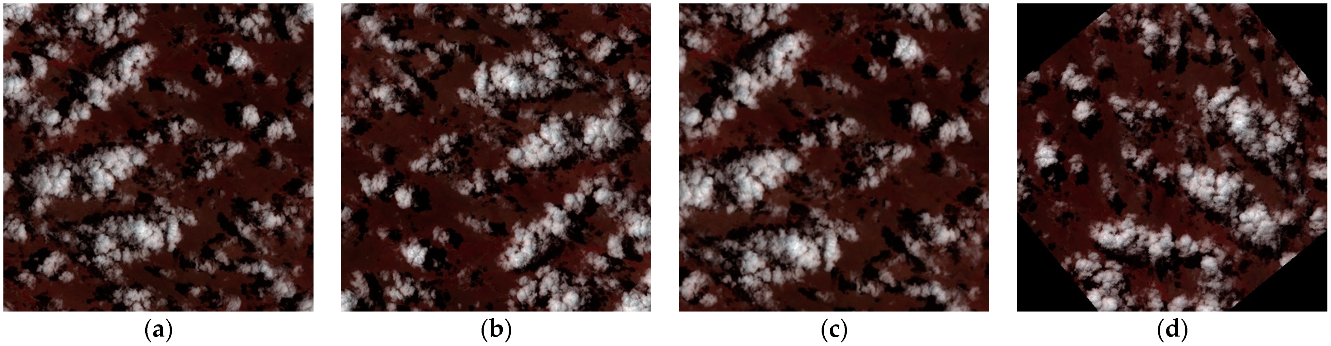
2.2. Data Pre-Processing

Chai et al. have pointed out that the cloud detection accuracy based on the top of the atmosphere is similar to that of the digital number value in deep learning [26]. In order to avoid the dependence on the complex calibration parameters of different satellite data, we use the digital number value images of RGB and NIR bands as training data and the manually labeled cloud masks of the L8 Biome as label data in our subsequent experiments.

The size of the L8 image is so large that it will cause a sharp increase in the amount of calculation when the large-size image is directly used as the network input. Limited by the hardware processing capabilities, we divide each L8 image into a set of non-overlapping sub-images and eliminate these sub-images containing filled pixels. Finally, we get about 12,000 sub-images. To conduct the follow-up experiments, we randomly divide these sub-images into the training set, the validation set, and the test set at a ratio of 6:1:3. The images in the training set are used for model training. The validation set is used to adjust parameters during the experiment. The test set is only used to evaluate the model performance and does not involve the training and parameter tuning processes. We also divide the images in the SPARCS set into sub-images.

At the same time, we use the data augmentation technology to increase the number and complexity of training samples in order to further improve the detection accuracy, generalization, and robustness of deep learning models. In this article, the training set is expanded 4 times by flipping, rotating, and scaling the image. Figure 1 shows the original image and the result of its data augmentation. From left to right in Figure 1, they are the original image, the flipping result, the scaling result, and the rotating result. The final training set contains 29384 images, the validation set contains 1176 images, and the test set contains 3672 images.

3. Methodology

The CD-AttDLV3+ introduces the semantic segmentation in deep learning into the cloud detection and achieves pixel-level cloud detection in this paper. Combining the spectrum, spatial information, and other deep feature information, the entire image is classified into two types of regions: cloud and surface. The CD-AttDLV3+ training and verification process is shown in Figure 2, and the pseudo-code of the process is shown in Algorithm 1. In our algorithm, we first segment the RGB and NIR images and manual cloud masks in the L8 Biome into sub-images with a size of 512 × 512. Then, we divide the sub-images into training set, validation set, and test set and perform data augmentation on the training set. Third, we use the training set to train the CD-AttDLV3+ to obtain the cloud detection model. Finally, we use the test set to evaluate the model performance and compare with other methods. In addition, the trained cloud detection model is applied to the L8 SPARCS dataset and the Sentinel-2 images to evaluate the extendibility of the model.

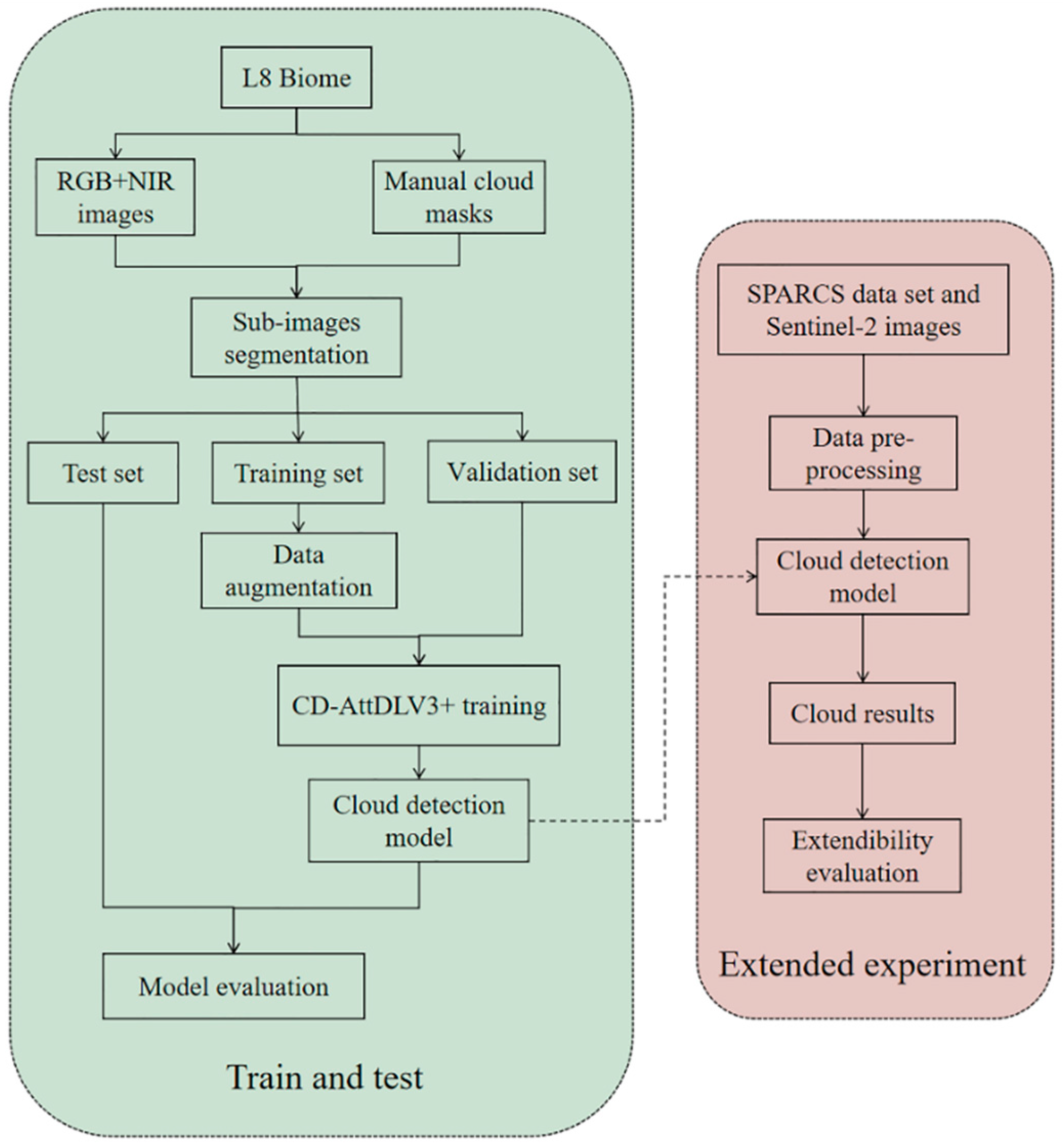
Algorithm 1 The CD-AttDLV3+ training and verification

Input:dataSet is data of L8 Biome; SPARCSimg and Sentinel2imgare the images for extended experiment; net is initial network; lr is learning rate; bs is batch size; algorithm SGD is named sgd; fl is focal loss function; iter is the number of iterations; maxiter is the maximum number of iterations Output: subimage set: subimageSet; trainSet, trainSetaug, testSet and valSet; trained model: modeliter; best trained model: modelbest; evaluation index: PRval, PRtest, RRtest, F1test, FWIoUtest; cloud detection results: testpredict, SPARCSpredict and Sentinel2predict 1: subimageSet ← cut images in dataSet with uniform size 2: (trainSet, testSet, valSet) ← split(subimageSet) 3: trainSetaug ← augment trainSet by flipping, rotating, and scaling 4: {Si|k = 1, 2,…, n} ← (split trainSet according to bs) 5: while iter < maxiter do 6:        netiter ← update net parameters with Si, lr, sgd, fl 7:        if iter%100 == 0 then 8:              PRval ← netiter evaluate valSet 9:              modeliter ← netiter 10:        end if 11: end while 12: modelbest ← choose the best model in modeliter using PRval 13: (testimg, testlabel) ← testSet 14: testpredict ← cloud detection for testimg using modelbest 15: PRtest, RRtest, F1test, FWIoUtest ← comparison of testpredict and testlabel 16: (SPARCSpredict, Sentinel2predict) ← cloud detection for SPARCSimg and Sentinel2imgusing modelbest

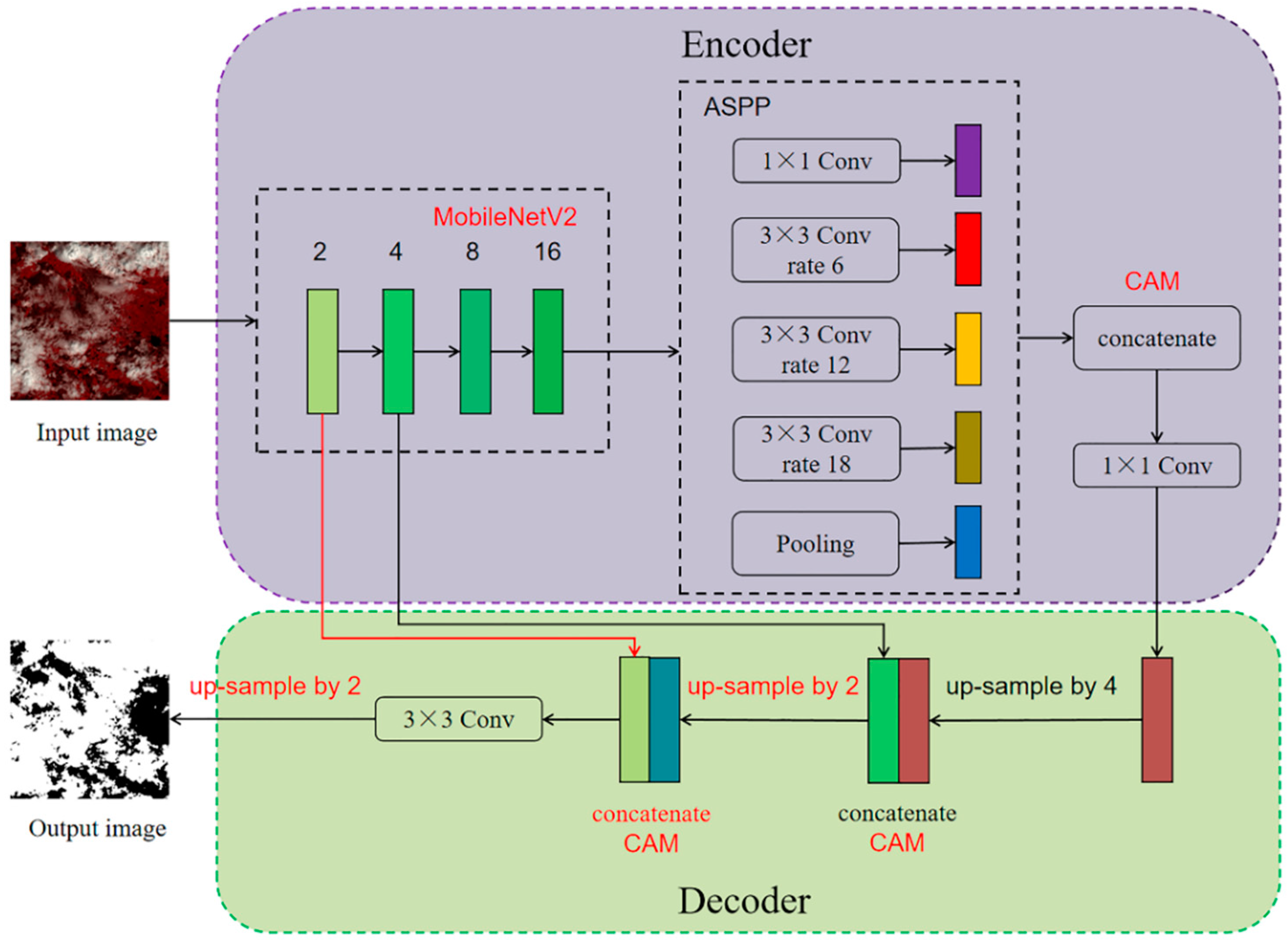
3.1. CD-AttDLV3+ Architecture

DeeplabV3+ adds a decoder on the basis of DeeplabV3 and realizes semantic segmentation by constructing the encoding–decoding structure. In the encoding stage, the input image first uses the backbone network to obtain the feature tensor of 2, 4, 8, and 16 times down-sampling. Then, we put the 16 times down-sampling feature tensor into the ASPP. Finally, the features obtained from the ASPP are spliced and compress the number of channels through a 1 × 1 convolution. In the decoding part, the feature tensor from the encoding part is up-sampled 4 times and concatenated with the same resolution features extracted from the backbone network. Finally, the size of the original image is restored by convolution and up-sampling, and the detection result is thereby obtained.

In order to be better used for cloud detection, the CD-AttDLV3+ retains the excellent encoding–decoding structure and the ASPP module in the DeeplabV3+. However, a series of improvements are implemented. Our CD-AttDLV3+ architecture is shown in Figure 3, and the improved part is marked in red. The input of the network is a sub-image of the RGB and NIR bands, and the output is a cloud distribution map. In the encoder stage, firstly, the light-weight network MobileNetV2 is used as the backbone network to reduce the computational load, so as to efficiently and quickly mine the multi-level image features. The MobileNetV2 can extract feature maps of 2, 4, 8, and 16 times down-sampling. Then, the ASPP module includes an average pooling layer with global information features, a 1 × 1 convolution for original scale features, and three 3 × 3 convolutions with hole ratios of 6, 12, and 18, respectively. By introducing three dilated convolutions of different sizes, the ASPP module obtains the convolution kernel with multiple receptive fields in the case of fewer parameters to extract features at different scales. In addition, the sizes of different feature maps at different scales can be kept the same to retain more location information. Finally, we concatenate the feature maps extracted by ASPP and compress the number of channels through a 1 × 1 convolution. In the decoder stage, the feature maps are restored to the original size of the input image through continuous up-samplings. To improve the segmentation effect of the cloud boundary and details, the CD-AttDLV3+ additionally concatenates 2 times down-sampling features in the decoding part to make use of more low-level location information. Moreover, the CAM is introduced to set different weight coefficients for different feature channels in the concatenate process. In this way, our CD-AttDLV3+ enhances the learning ability and generalization ability by strengthening the pertinence of learning.

3.1.1. Light-Weight Backbone Network

MobileNet is a light-weight network model for mobile devices and embedded devices. Its outstanding contribution is to replace standard convolution with deep separable convolution, which greatly reduces the model’s computational effort [40]. The deep separable convolution decomposes the standard convolution into two convolutions. For the first time, the input feature is convolved with the convolution kernel of channel number 1 for feature extraction, which is called deep convolution. For the second time, the result of the first convolution is convolved with the 1 × 1 convolution kernel of the expanded channel number, which is called point convolution. The 3 × 3 deep separable convolution reduces the computation 8 to 9 times, comparing to the standard convolution with only a slight reduction in accuracy [40]. On the basis of the deep separable convolution, the MobileNetV2 introduces the inverted residual structure to further improve the network performance [41]. For the residual module, the input feature channels are first compressed by 1 × 1 convolution. Then, the compressed channels use 3 × 3 convolution for information extraction. Finally, the number of channels is restored by 1 × 1 convolution. This mode of “compression–convolution–expansion” reduces the computational amount and improves the computational efficiency. However, when the feature channels are first compressed, the extracted information suffers a great loss. Therefore, our inverted residual module adopts the calculation mode of “expansion–convolution–compression” to extract rich information and improve the accuracy.

In this paper, the improved light-weight MobileNetV2 is our backbone network, whose architecture is shown in

Table 1. The backbone network structure.

Input	Operator	t	c	n	s
5122 × 3	conv2d	-	32	1	2
2562 × 32	bottleneck	1	16	1	1
2562 × 16	bottleneck	6	24	2	2
1282 × 24	bottleneck	6	32	3	2
1282 × 32	bottleneck	6	64	4	2
642 × 64	bottleneck	6	96	3	1
642 × 96	bottleneck	6	160	3	1
642 × 160	bottleneck	6	320	1	1

. Herein, the Input represents the size of the input feature map of this layer. The Operator represents the operation performed by the network, including the convolutional layer and the inverted residual structure. The t is the expansion multiple of channels in the inverted residual module. The c is the number of output channels. The n is the number of repetitions for the current layer. The s is the stride of the inner convolution in the current layer. First of all, in order to reduce the computational load and the memory occupancy of the network, only the first eight layers of MobileNetV2 are retained in this paper, which effectively avoids the significant increase in the channel number and the large consumption of computing resources. Secondly, the original MobileNetV2 is aimed at the image classification task, and the sizes of the output feature maps in the eighth layer are 1/32 of the original image. In order to make it adapt to our cloud detection CD-AttDLV3+ and increase the feature sizes to 1/16 of the original image, the stride size of the seventh layer is changed to 1.

3.1.2. Channel Attention Module

In the deep learning calculation process, different channels go through different computing processes and contain different feature information, which makes different contributions to the subsequent image segmentation. There are multiple channel concatenate processes in the CD-AttDLV3+. In order to highlight the channels with significant contributions, suppress the channels with small contributions or information redundancy, and strengthen the pertinence of subsequent learning, we introduce the CAM and assign different weights to different channels.

The architecture of the CAM is shown in Figure 4. The input is the feature with a size of H × W × C. H and W represent the length and width of the input feature, respectively. C represents the number of channels. Firstly, the input features are compressed into the size of 1 × 1 × C through the global average pooling. Then the weight coefficients of each feature are obtained through two full-connection (FC) layers with up-sampling and down-sampling. Finally, the weight coefficients are multiplied by the corresponding input features to realize the weighted allocation of features in different channels [42]. This algorithm for calculating weights for different features allows the network to pay more attention to the more significant features during the training process, thereby improving the accuracy and the training speed.

3.2. Improved Loss Function

The sample imbalance is a common phenomenon in deep learning. In the semantic segmentation process of deep learning for cloud detection, this imbalance is even more apparent. On the one hand, semantic segmentation belongs to pixel-level classification, and pixel numbers between categories in images usually vary greatly. Especially in remote sensing images, clouds are generally in a sizeable continuous coverage rather than evenly distributed on the surface. As a result, a sub-image often contains a lot of clouds or surfaces. The number of pixels in one category is usually several or even dozens of times higher in another category. The sample size is severely imbalanced, and this level of sample imbalance is often difficult to balance by training strategies. On the other hand, the thick cloud is easy to distinguish from the ordinary surface. However, some bright surfaces, such as snow, ice, and bright buildings, are easily confused with clouds. Thin light-transmitting clouds are also difficult to detect because they usually have a low brightness and some surface information.

In order to alleviate a series of problems caused by the sample imbalance, we tried our best to ensure the balance of samples between different categories during the production of the dataset. In addition, different learning difficulties of different samples also lead to imbalance, so adjusting the weight of the loss value and focusing on the training of the difficult samples can also alleviate the sample imbalance problems. Therefore, we introduced a loss function to our algorithm that can automatically adjust the weight according to the difficulty of sample learning.

Focal loss is a typical loss function to alleviate sample imbalance in two-stage target detection, and it is improved by cross entropy. Focal loss adjusts the weight of the loss value according to the difficulty degree of the sample and makes the network prone to learning difficult samples [43]. Equation (1) is the calculation formula for cross entropy, and Equation (2) is the calculation formula for focal loss.

$$CE=-\log P_t$$

(1)

$$FL=-{(1-P_t)}^{\gamma }\log P_t$$

(2)

where P_t represents the probability of model prediction, and the weight γ adjusts the decrease rate of the sample weight. When γ is set to 0, the focal loss function degenerates into a cross-entropy loss function. When γ increases, the adjustment factor also increases.

The original focal loss function achieves the targeted training by suppressing the loss value of samples to different degrees. The suppression makes the weight of the sample loss value fall in the interval of 0 to 1. The weights of easy samples are close to 0, and the weights of difficult samples are close to 1, but in the process of semantic segmentation, we need to classify each pixel correctly. Therefore, while retaining the loss value weights of easy samples, increasing the loss value weights of difficult samples is more suitable for semantic segmentation. The focal loss function of our CD-AttDLV3+ is as follows:

$$F{L}_{CD-AttDLV3+}=-{(2-P_t)}^{0.5}\log P_t$$

(3)

4. Experimental Results

In this section, we evaluate the proposed CD-AttDLV3+. Specifically, we first verify the network structure through its performance on the verification set. Furthermore, to evaluate the effectiveness, we use the CD-AttDLV3+ to perform cloud detection on the test set and compare it with typical methods, including the threshold-based Fmask method [7], the SVM method [12], and the SegNet based on deep learning [16]. The comparison process includes two parts: qualitative evaluation and quantitative evaluation. In addition, the CD-AttDLV3+ only uses the most common RGB and NIR bands of optical remote sensing images for cloud detection, which lays the foundation for extendibility. In order to verify the extendibility of the CD-AttDLV3+, we use the trained cloud detection model to perform cloud detection on the SPARCE set and Sentinel-2 images.

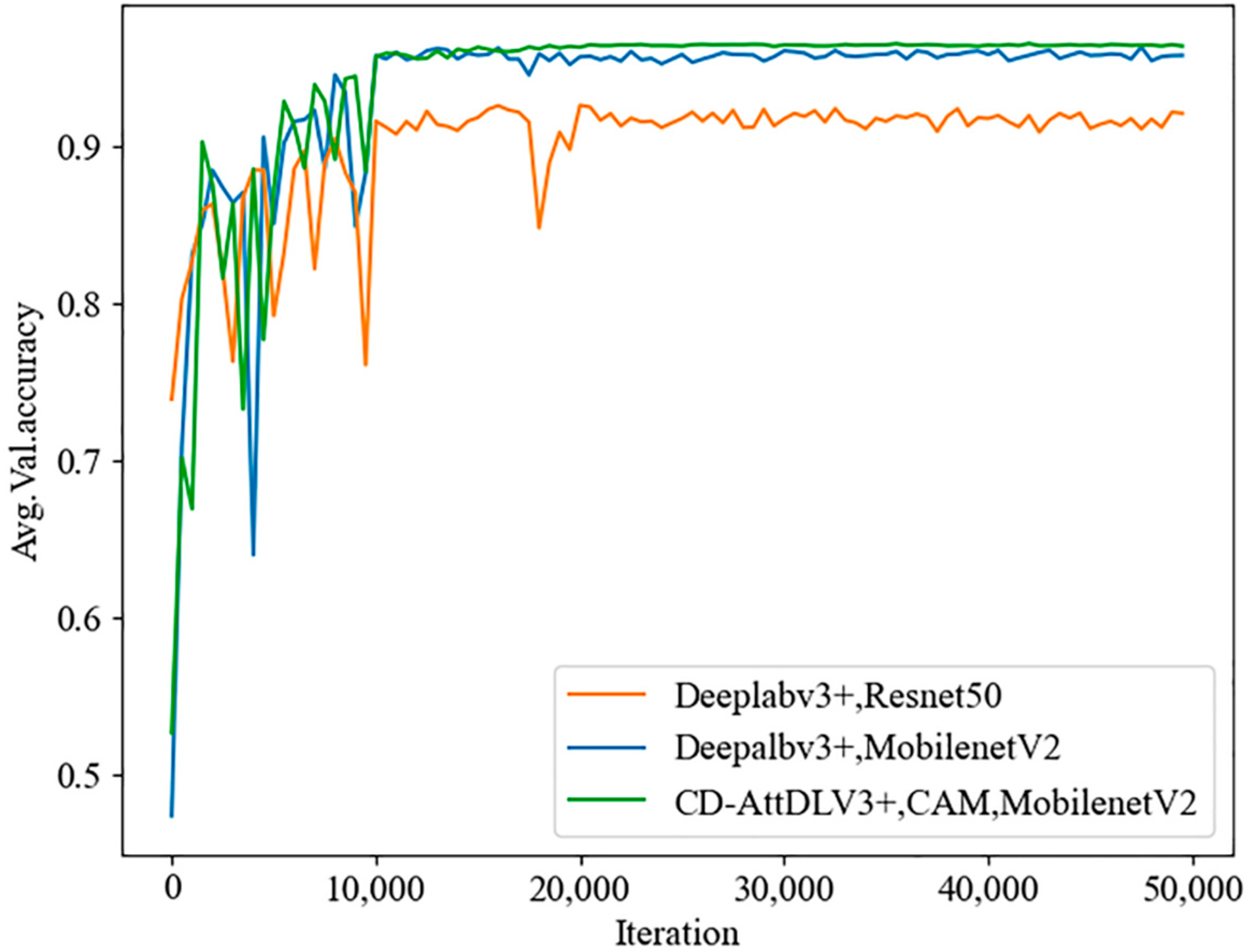
4.1. Network Architecture Validation

The network model contains many parameters. The training of deep learning is a process that includes a continuous iteration and adjustment of model parameters to minimize the difference between the label and the predicted result. We use the stochastic gradient descent (SGD) optimizer with the focal loss function and input 16 images in each batch for training. Moreover, the experiment also adds the dropout, which prevents the model from over-fitting by inactivating neurons.

The original DeeplabV3+ and the CD-AttDLV3+ are trained based on the same training dataset and verified on the same validation dataset. The accuracy curves over the validation dataset of different networks are shown in Figure 5.

Table 2. Comparison of parameter quantity and accuracy for different combinations.

Model Architecture	Backbone Network	Parameter Quantity	Accuracy
DeeplabV3+	Resnet50	3.98 × 107	0.9172
DeeplabV3+	MobilenetV2	5.22 × 106	0.9582
CD-AttDLV3+	MobilenetV2	5.56 × 106	0.9644

shows the number of parameters and the accuracy of the verification set with different models and backbone networks. In Table 2, the Model architecture includes the original structure of DeeplabV3+ and our CD-AttDLV3+ structure. The Backbone network includes Resnet50 and MobilenetV2. The Parameter quantity represents the parameter quantity of the entire network under different combinations. The Accuracy is the maximum value of accuracy obtained by different combinations of networks on the verification set. According to Figure 5 and Table 2, it can be seen that the MobilenetV2 can effectively reduce the number of parameters and obtain a higher accuracy. The CD-AttDLV3+ has a slight increase in the number of parameters due to the CAM and more low-level features, but the accuracy of the validation set is also improved.

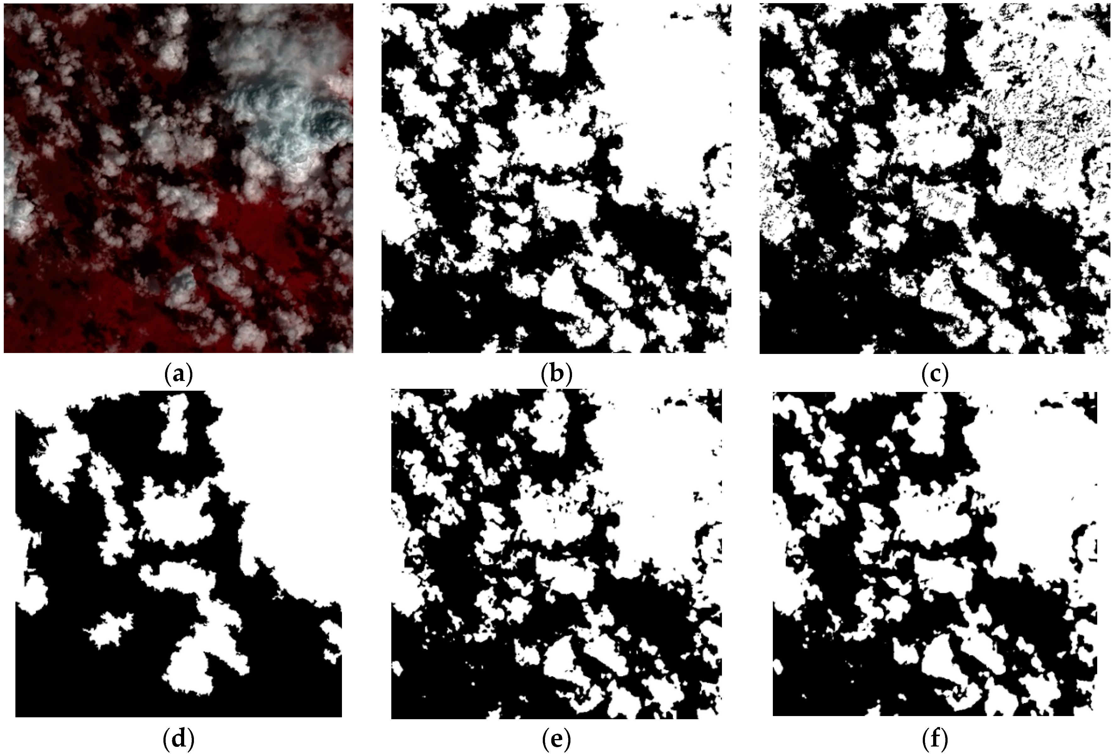
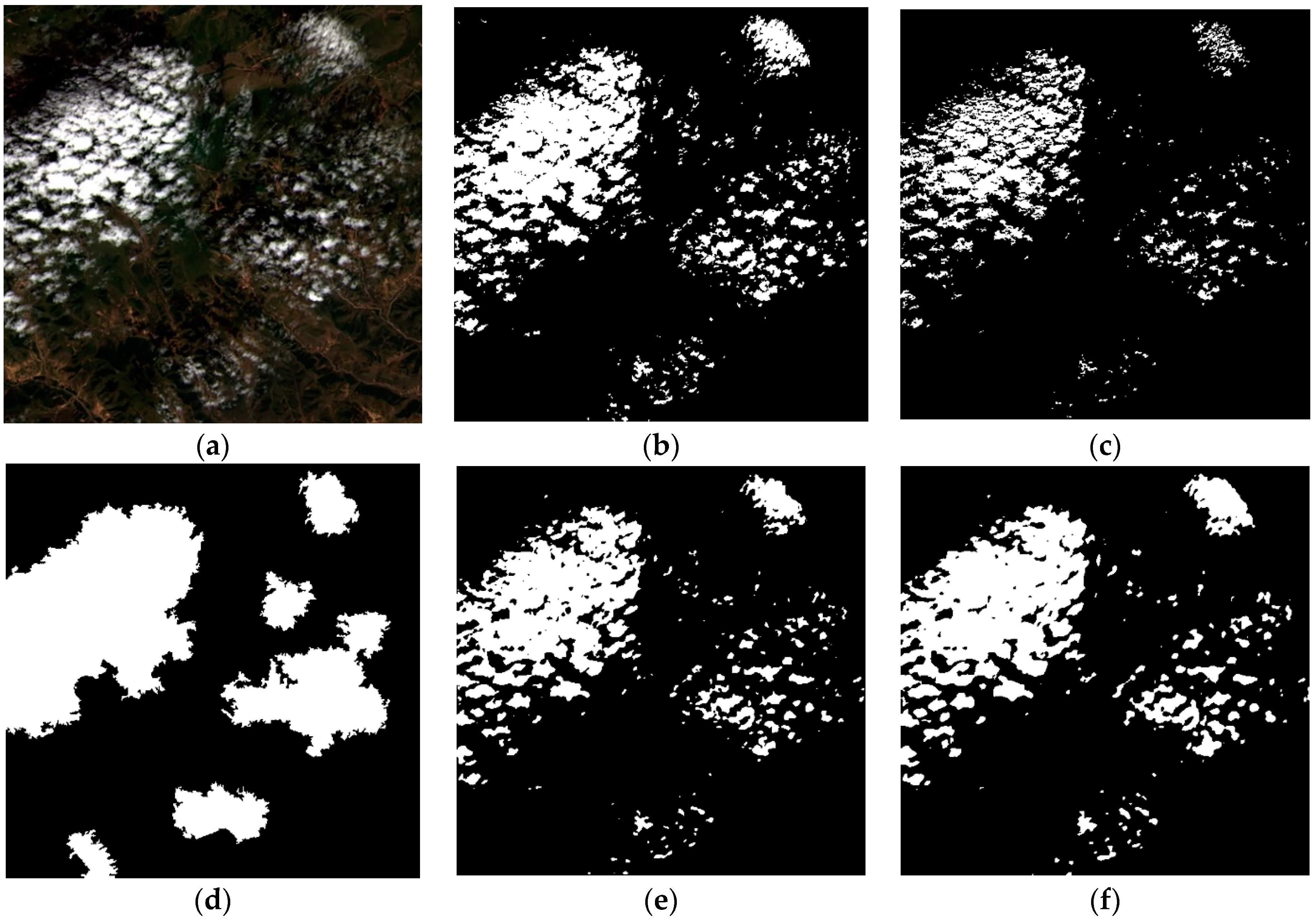
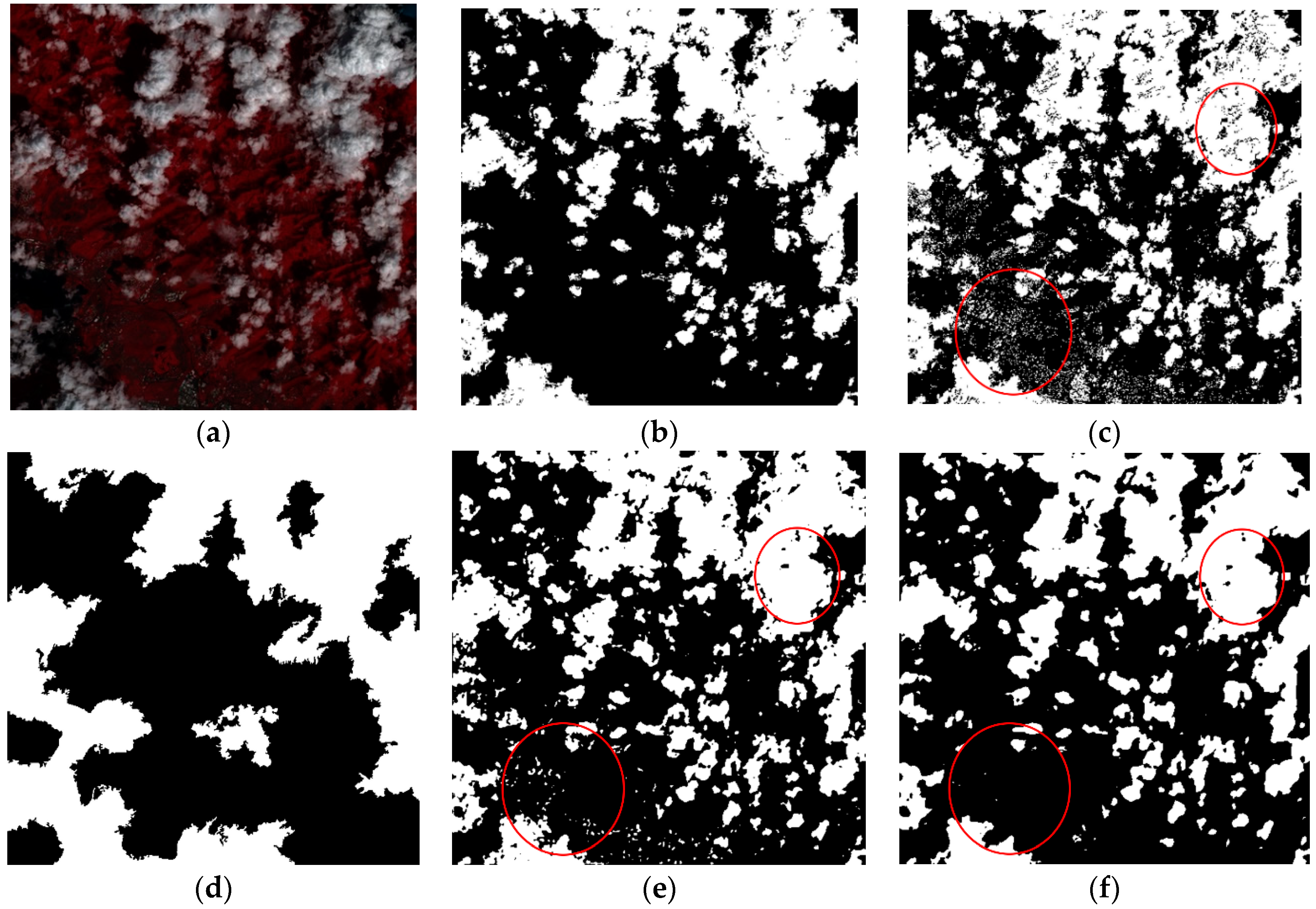
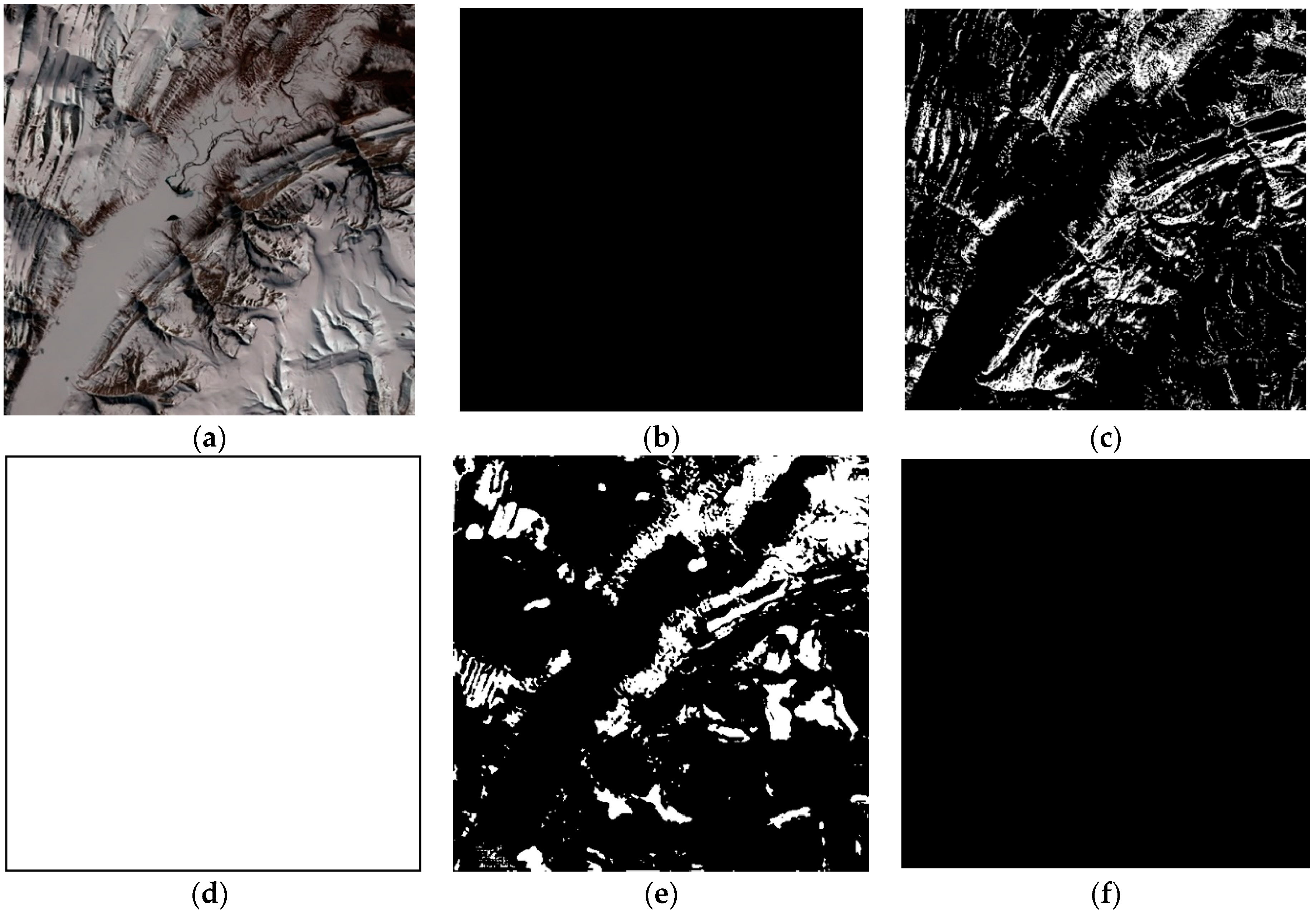
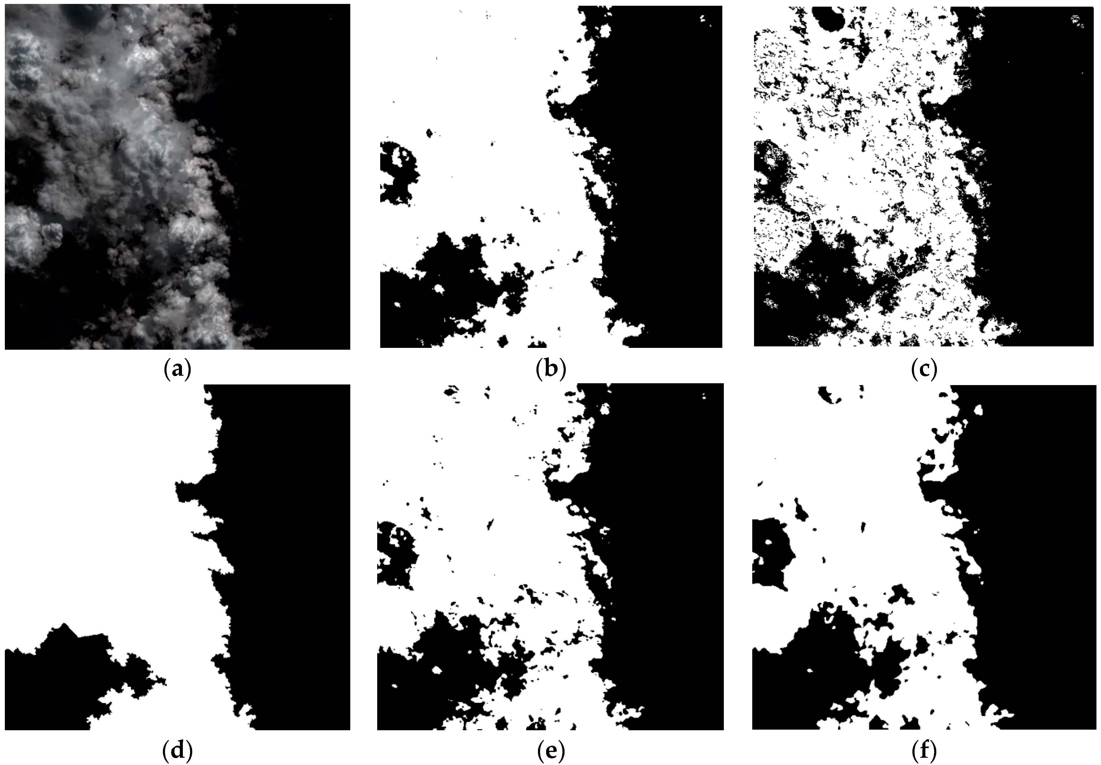
4.2. Qualitative Evaluation

We selected representative images from eight kinds of surfaces with barren, forest, grass, urban, snow, shrubland, wetlands, and water in the test set for visual evaluation. Figure 6, Figure 7, Figure 8, Figure 9, Figure 10, Figure 11, Figure 12 and Figure 13 are the different cloud detection results of these eight surfaces. These figures sequentially show the original images, the manually generated cloud masks, the Fmask method results, the SVM method results, the SegNet results, and our CD-AttDLV3+ results.

In Figure 6, with the barren surface, four methods detect most of the cloud. However, the Fmask method has some missed-judgments inside the cloud, and cloud boundaries have also shown varying degrees of degradation (See Figure 6c). Since the Fmask performs cloud detection pixel by pixel, the result obtained is relatively fragmentary. The SVM method mistakenly incorporates some gaps into the cloud. The reason for this misjudgment is that clouds and surfaces are incorrectly classified as the same super-pixel. This phenomenon is common when there are many broken clouds in images. Although the SegNet method has obtained more accurate cloud results, there are still three misjudgments in the position of the red circles (See Figure 6e). The result of the CD-AttDLV3+ has no obvious misjudgment and is the closest to the manually generated cloud mask. In Figure 7, with the forest surface, the result of the Fmask has the same problem, as some holes appear inside the cloud. There are some broken clouds in Figure 8 that make it difficult for the SVM method to fit the actual cloud boundary during super-pixel segmentation, which leads to some misjudgments in the results. The low left part of Figure 9 is an urban area, and the brightness is relatively high. The results of the Fmask and the SegNet have some misjudgments. In the results of the Fmask method, there is a large number of misjudgments, but the CD-AttDLV3+ avoids this phenomenon well (see the red circles in Figure 9c,e,f). Figure 10 shows a large snow area with a weak texture. The SVM method misjudges the whole scene image. The results of the Fmask and the SegNet also show some misjudgments. Only the CD-AttDLV3+ completely excludes the snow. In Figure 11, Figure 12 and Figure 13, the cloud detection results of the CD-AttDLV3+ are also the closest to manually generated cloud masks.

In summary, all four methods can achieve high-quality visual performances and distinguish most of the cloud from the surface. However, from the above comparison details, it can be seen that the cloud detection results of our CD-AttDLV3+ are the closest to the manually generated cloud masks. The Fmask is a pixel-by-pixel cloud detection method, so noise is prone to appear in the detection result, in the form of holes in the cloud area or sporadic cloud points on the surface. Especially in the detection process, it is easy to interfere with bright surfaces such as an urban area and snow. In addition, the Fmask uses more band information and is more dependent on the spectral information of the image. The SVM method first performs super-pixel segmentation on the image and then classifies the super-pixels to realize cloud detection. The detection results of the SVM depend to a large extent on the effect of super-pixel segmentation. Therefore, the method is not sensitive to the broken cloud with a small area, and a misjudgment can easily occur when there is a large number of broken clouds in the image. Moreover, the SVM only uses the RGB and NIR bands, so it mainly relies on local texture features to distinguish the cloud from the bright surface. When the texture information of the bright surface is weak, misjudgments are liable to occur. As for the benefits from the accurate extraction and the learning of deep features from numerous samples, the remaining two deep learning methods are significantly better than the first two methods. Moreover, when bright surfaces are covered, the anti-interference ability of the CD-AttDLV3+ is stronger than that of the SegNet. As shown in Figure 9 and Figure 10, the CD-AttDLV3+ can accurately identify the bright surfaces, while the SegNet misjudges a part of the bright surfaces as clouds. The main reason is that CD-AttDLV3+ can more fully extract the context information in the image at the multi-scale. The ASPP module is introduced to extract the multi-scale information while effectively solving the information loss caused by multiple down-sampling in the SegNet. In addition, the improved loss function can also improve the detection effect of challenging pixels like bright surfaces by increasing the proportion of the loss of challenging pixels. Therefore, the CD-AttDLV3+ can generate more precise and more accurate cloud detection results in a qualitative evaluation. It has a more vital anti-interference ability, especially in complex surfaces.

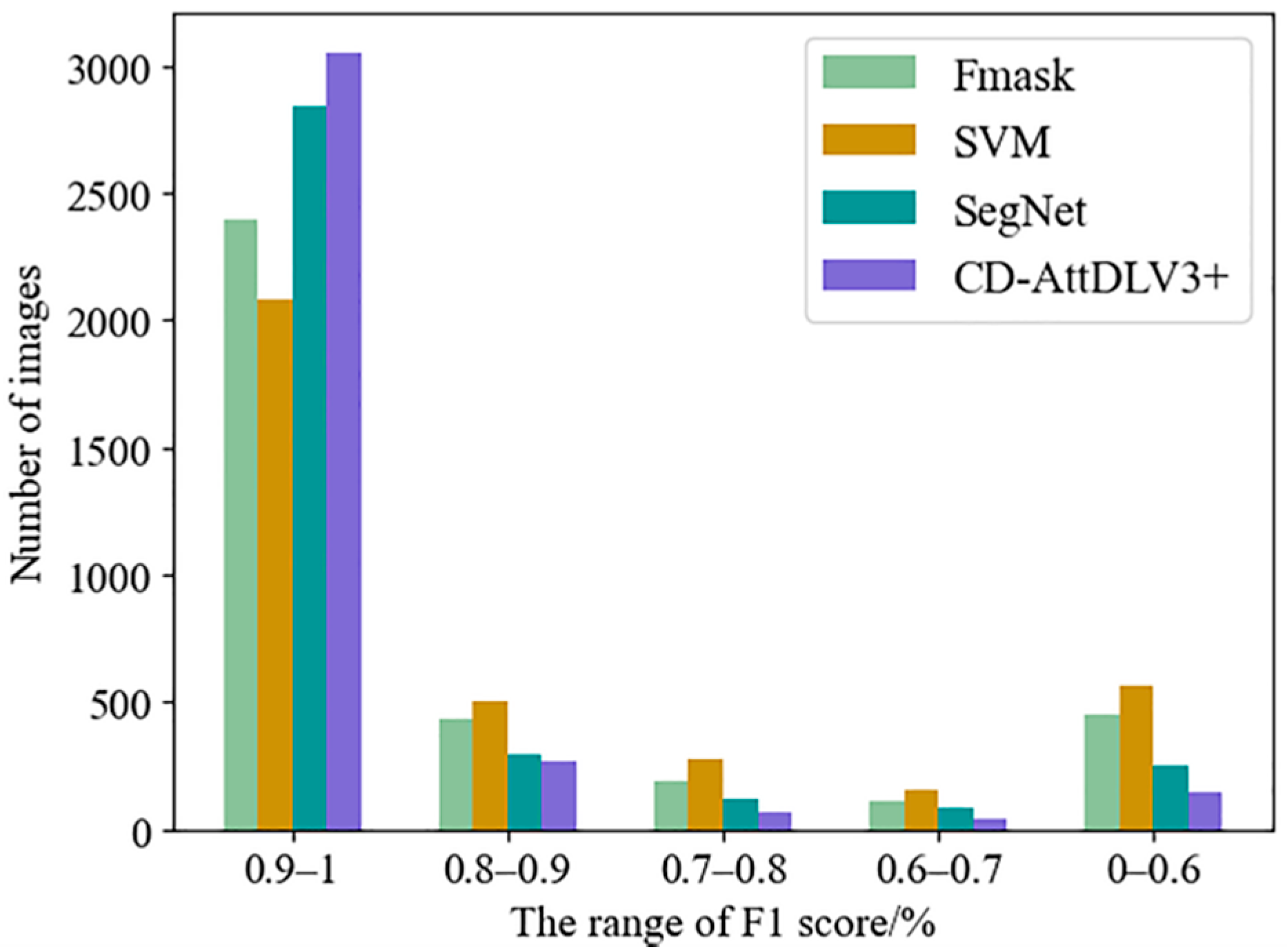
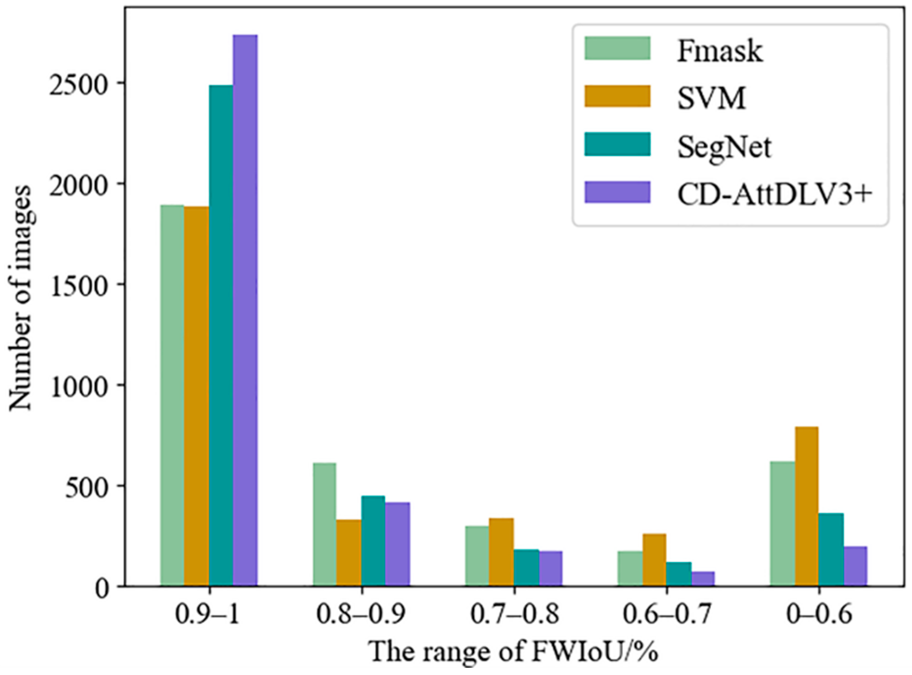
4.3. Quantitative Evaluation

In order to further verify the effectiveness and feasibility of the CD-AttDLV3+, we perform the quantitative evaluation by calculating the accuracy evaluation indicators on the test set. The accuracy evaluation indicators include the precision ratio (PR), the recall ratio (RR), the F₁ score, and the frequency-weighted intersection over union (FWIoU). The PR represents the ratio of the correct number of cloud pixels in the detection result to the number of cloud pixels in the detection result. The RR represents the ratio of the number of correct cloud pixels in the detection result to the number of cloud pixels in the manually generated cloud mask. The F₁ score integrates PR and RR. The higher the F₁ score, the better the result of the model prediction. The FWIoU is improved by IoU, and it sets weights for different types of IoU according to the frequency of pixel appearance. The calculation of each evaluation indicator is as follows.

$$PR=\frac{TP}{TP+FP}$$

(4)

$$RR=\frac{TP}{TP+FN}$$

(5)

$$F_1=\frac{2\times PR\times RR}{PR+RR}$$

(6)

$$FWIoU=\frac{TP+FN}{Total}\times \frac{TP}{TP+FP+FN}+\frac{TN+FP}{Total}\times \frac{TN}{TN+FP+FN}$$

(7)

where TP (true positive) and TN (true negative) denote the total number of cloud pixels and non-cloud pixels correctly predicted, respectively. FP (false positive) and FN (false negative) denote the total number of pixels with an incorrect outcome from the cloud and non-cloud recognition, respectively. Total denotes the total number of pixels.

Table 3. Quantitative evaluation results of different methods.

Methods	PR	RR	F1	FWIoU
Fmask	0.9348	0.8245	0.8762	0.7967
SVM	0.8828	0.8054	0.8424	0.7670
SegNet	0.9499	0.9011	0.9249	0.8742
CD-AttDLV3+	0.9586	0.9414	0.9499	0.9151

Note: Bold numbers are the best results.

shows the evaluation results of different cloud detection methods. The numbers in bold in Table 3 express the maximum values of the corresponding index. It can be seen that two deep learning methods have obvious advantages. This is mainly because these deep learning methods can fully extract the spectrum, texture, and other informations in the image and automatically learn the deep features in the training data. Moreover, these deep learning methods can make decisions at multiple levels to improve the accuracy of cloud detection. Although the threshold-based Fmask method combines multiple band information of visible light and infrared, it still has deficiencies in the cloud, snow separation, and cloud boundary maintenance. The SVM method has a good detection effect on areas with high vegetation coverage, but its detection results depend on the effect of the super-pixel segmentation. For some areas with broken clouds, it is usually difficult for super-pixels to fit the boundary. Moreover, this method is difficult to distinguish between clouds and the weakly textured bright surface.

For the two deep learning methods, it can be seen that all evaluation indicators of the CD-AttDLV3+ are improved comparing to the SegNet, in which the PR increased by 0.0087, the RR increased by 0.0403, the F₁ score increased by 0.025, and the FWIoU increased by 0.0409. The main reason is that the CD-AttDLV3+ benefits from the excellent encoding–decoding structure of the DeeplabV3+. By introducing ASPP, the CD-AttDLV3+ fully extracts the multi-scale information in the image and enlarges the receptive field without changing the image resolution. The introduction of ASPP also effectively avoids the problem of target boundary information loss caused by multiple down-sampling in the SegNet.

In order to further evaluate the detection effects of different methods, we divide the F₁ score and the FWIoU into five intervals (0–0.6, 0.6–0.7, 0.7–0.8, 0.8–0.9, 0.9–1) and obtain statistical results for each interval. As shown in Figure 14 and Figure 15, the statistical results of the four methods are displayed in four different colors. In Figure 14 for the F₁ score, the four methods have the largest number of images falling in the 0.9–1 interval. In particular, the number of our CD-AttDLV3+ is higher than those of the other three methods. This shows that the four methods can get superior detection results in most cases, while the comprehensive detection effect of our CD-AttDLV3+ is the best. As the F₁ score decreases, the number of images in the corresponding interval gradually decreases until the interval 0–0.6 rises. This is mainly because the range of this interval is larger than that of the other intervals. On the other hand, most of images falling within this interval contain large areas of snow or other bright surfaces, prone to large-scale misjudgments. However, the number of images falling within this interval for the CD-AttDLV3+ is the smallest. The distribution trend of the number of images in Figure 15 is basically the same as that in Figure 14, which confirms the above conclusion.

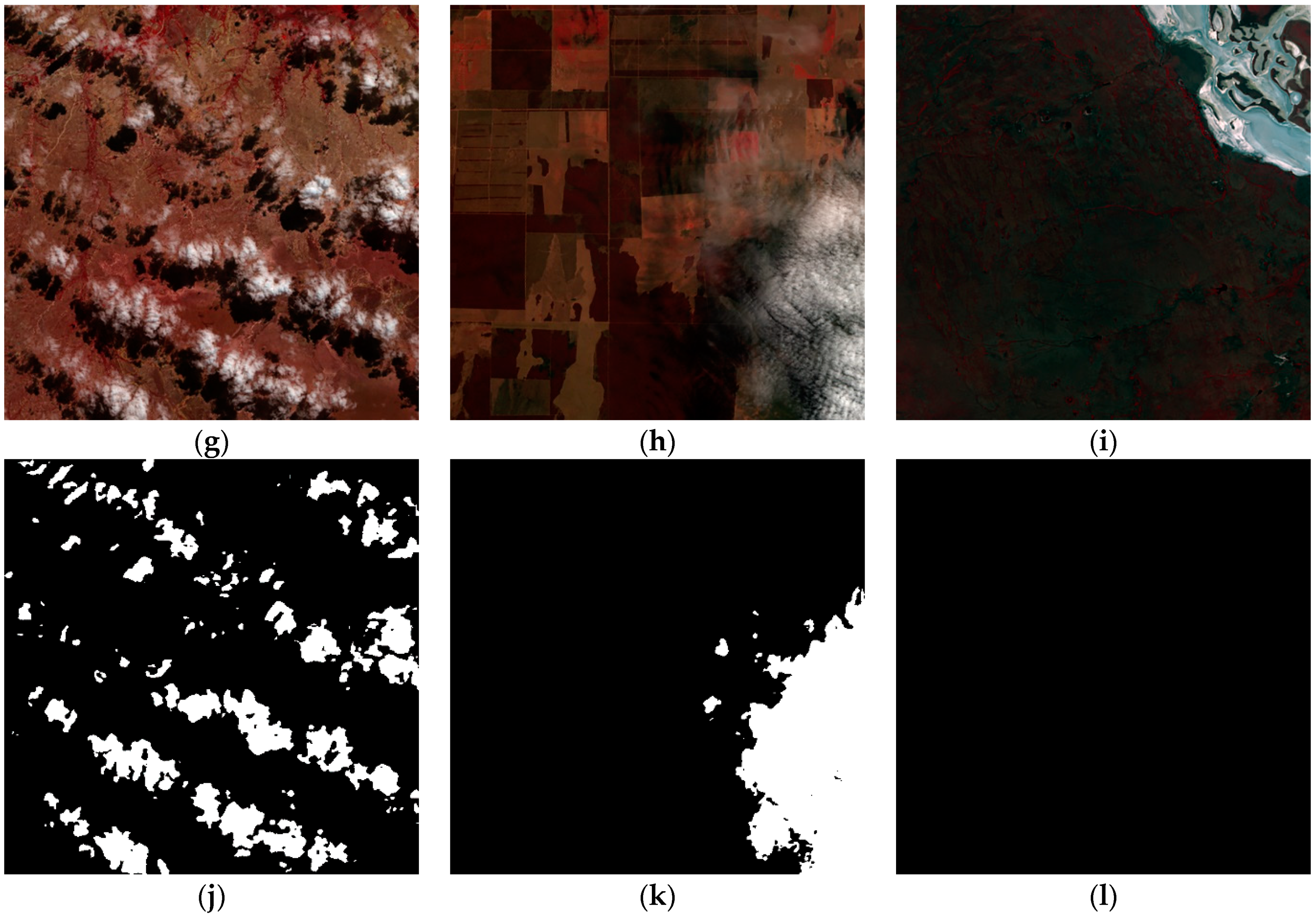
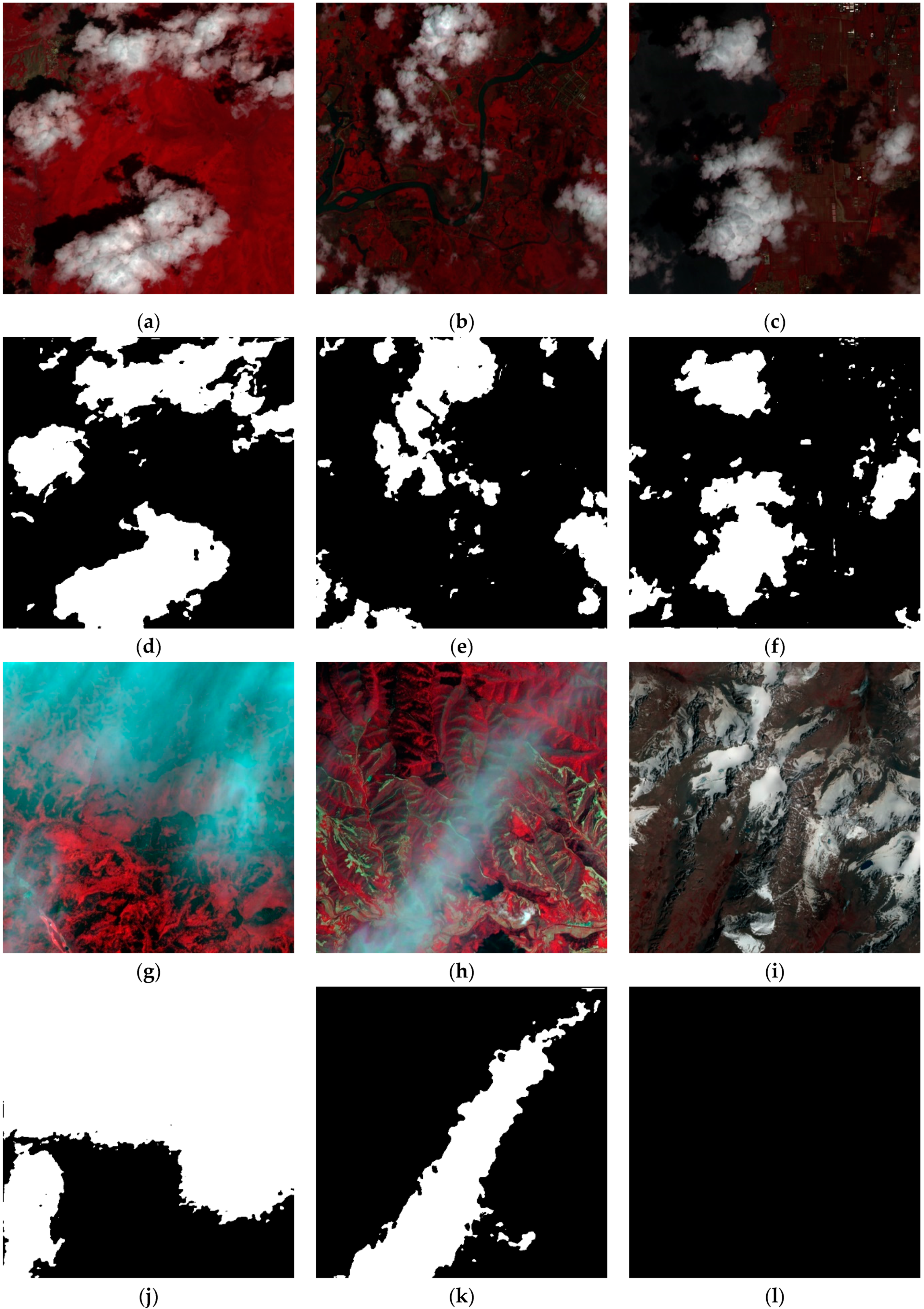
4.4. Extended Experiment

Deep learning usually has a stronger generalization ability than traditional methods. Moreover, the CD-AttDLV3+ only uses the RGB and NIR bands to realize the cloud detection, and it is less dependent on band information. In this section, we directly apply the CD-AttDLV3+ model trained on the L8 Biome to the SPARCS set to verify the extendibility on different datasets of L8. Then, we use the trained model to perform cloud detection on the Sentinel-2 images to verify the extendibility of different sensor data.

4.4.1. The SPARCS Set Cloud Detection

In this section, we use the CD-AttDLV3+ to perform cloud detection on the cropped sub-images from the SPARCS set. Some representative results are shown in Figure 16.

Figure 16a,b and their results show that the CD-AttDLV3+ has good detection results on surfaces with high vegetation coverage. Not only the thick cloud, but also some small broken clouds in images are fully detected. The cloud boundary is well maintained. Moreover, most of the light-transmitting thin cloud is also detected in Figure 16c, although it contains some surface information. The vegetation coverage in Figure 16g is relatively low. The CD-AttDLV3+ still achieves good detection results, and there is no obvious misjudgment or missed-judgment. Figure 16h shows a missed-judgement regarding a thin cloud in the right side of the image. The main reason may be that there is no sample similar to this kind of light-transmitting thin cloud in the training set. Finally, some of the high-brightness ice and snow in Figure 16i are effectively eliminated from the clouds.

In general, the CD-AttDLV3+ has a strong extendibility among different datasets of the same sensor. The CD-AttDLV3+ can achieve valid results for difficult-to-detect areas in the SPARCS dataset, such as bright ice, snow, and light-transmitting thin clouds. However, the detection performance may slightly decrease due to differences in the time and location of image acquisition in different datasets. Therefore, establishing a more comprehensive and practical training dataset can help further improve the detection effect of the CD-AttDLV3+.

4.4.2. Sentinel-2 Cloud Detection

The Sentinel-2 multispectral imager (MSI) has 13 channels, of which the RGB and NIR bands are bands 2/3/4/8, and the spatial resolution is 10 m. The spectral range and the spatial resolution of Sentinel-2 are different from those of L8, which more fully validates the extendibility of the model.

Figure 17 illustrates six typical examples of the original images and the CD-AttDLV3+ results for Sentinel-2 imagery on different surface types. It can be seen from Figure 17a that the CD-AttDLV3+ has an excellent detection effect in the area with high vegetation coverage. Figure 17b,c shows an urban area with relatively low vegetation coverage. The CD-AttDLV3+ detects most clouds, and there is no apparent missed-judgment. But in Figure 17c, a small part of the high-brightness buildings is misjudged as the cloud. From Figure 17g,h, it can be seen that the CD-AttDLV3+ works well for some light-transmitting thin clouds which are hard to detect. In Figure 17i, the CD-AttDLV3+ effectively excludes snow which is easily confused with the cloud.

In general, the CD-AttDLV3+ can achieve high-quality visual performances in the cloud detection of Sentinel-2. This shows that it has a strong extendibility on different sensor data, although there are some differences in the spectral range, spectral response function, and spatial resolution. This extendibility also proves the possibility of using the existing dataset to quickly develop cloud detection models for new sensor images.

5. Discussion and Conclusions

In this paper, we propose a deep learning cloud detection method based on the DeeplabV3+ architecture and the CAM (CD-AttDLV3+) to fully excavate deep features of images and improve the detection accuracy. We first improve the expansibility and applicability by using only the most common RGB and NIR bands and increase the degree of automation by introducing deep learning without the difficult threshold selection. Secondly, we optimize the network architecture by using a light-weight network-MobilenetV2 as the backbone network to reduce the number of parameters, replacing the standard convolutions with deep separable convolutions, integrating more low-level features in the decoding stage to improve the cloud boundary quality, and introducing the CAM to improve the network learning efficiency. Finally, the loss function is improved to alleviate the imbalance problem of the samples and improve the detection effect of difficult samples such as thin clouds and bright surfaces.

In the qualitative and quantitative evaluation, we compare CD-AttDLV3+ with the other three methods of the Fmask, the SVM, and the SegNet. The results show that CD-AttDLV3+ is suitable for most situations. Especially when distinguishing a bright surface and a cloud, the detection effect is greatly improved compared with other methods. In the cloud boundary area, the results of the CD-AttDLV3+ are closer to the manual cloud distribution. The results of the extended experiment show that the CD-AttDLV3+ can also obtain good cloud detection results on other L8 images and Sentinel-2 images. In general, the CD-AttDLV3+ has a strong feasibility, accuracy, and extendibility in the cloud detection of optical remote sensing images and is a new and intelligent cloud detection method.

Although the CD-AttDLV3+ has a very competitive performance, its detection effect largely depends on the quantity and quality of the dataset. This is because the deep learning method is a data-driven method. In the future, we will try to establish a larger and richer training dataset to further improve the versatility of the model. At the same time, we should further optimize the model, balance the detection efficiency and accuracy, and apply it to the actual business processing of remote sensing data. In addition, cloud shadows affect the quality of the information extracted from the images, and cloud shadow detection is a significant but challenging task. In the future, we will incorporate cloud shadow detection into our research.

References

1. Ju, J.; Roy, D.P. The availability of cloud-free Landsat ETM+ data over the conterminous United States and globally. Remote Sens. Environ. 2008, 112, 1196–1211. [Google Scholar] [CrossRef]
2. Hou, S.W.; Sun, W.F.; Zheng, X.S. Overview of cloud detection methods in remote sensing images. Space Electron. Technol. 2014, 11, 68–76. [Google Scholar] [CrossRef]
3. Irish, R.R. Landsat 7 automatic cloud cover assessment. Algorithms for Multispectral, Hyperspectral, and Ultraspectral Imagery VI. Int. Soc. Opt. Photonics 2000, 4049, 348–355. [Google Scholar] [CrossRef]
4. Irish, R.R.; Barker, J.L.; Goward, S.N.; Arvidson, T. Characterization of the Landsat-7 ETM+ automated cloud-cover assessment (ACCA) algorithm. Photogramm. Eng. Remote Sens. 2006, 72, 1179–1188. [Google Scholar] [CrossRef]
5. Wu, X.; Cheng, Q. Study on methods of cloud identification and data recovery for MODIS data. Remote Sensing of Clouds and the Atmosphere XII. Int. Soc. Opt. Photonics 2007, 6745, 67450P. [Google Scholar] [CrossRef]
6. Zhu, Z.; Woodcock, C.E. Object-based cloud and cloud shadow detection in Landsat imagery. Remote Sens. Environ. 2012, 118, 83–94. [Google Scholar] [CrossRef]
7. Zhu, Z.; Wang, S.; Woodcock, C.E. Improvement and expansion of the Fmask algorithm: Cloud, cloud shadow, and snow detection for Landsats 4–7, 8, and Sentinel 2 images. Remote Sens. Environ. 2015, 159, 269–277. [Google Scholar] [CrossRef]
8. Qiu, S.; Zhu, Z.; He, B. Fmask 4.0: Improved cloud and cloud shadow detection in Landsats 4–8 and Sentinel-2 imagery. Remote Sens. Environ. 2019, 231, 111205. [Google Scholar] [CrossRef]
9. Sun, L.; Wei, J.; Wang, J.; Mi, X.; Guo, Y.; Lv, Y.; Yang, Y.; Gan, P.; Zhou, X.; Jia, C.; et al. A universal dynamic threshold cloud detection algorithm (UDTCDA) supported by a prior surface reflectance database. J. Geophys. Res. Atmos. 2016, 121, 7172–7196. [Google Scholar] [CrossRef]
10. Shao, Z.; Pan, Y.; Diao, C.; Cai, J. Cloud detection in remote sensing images based on multiscale features-convolutional neural network. IEEE Trans. Geosci. Remote Sens. 2019, 57, 4062–4076. [Google Scholar] [CrossRef]
11. Shan, N.; Zheng, T.; Wang, Z. High-speed and high-accuracy algorithm for cloud detection and its application. J. Remote Sens. 2009, 13, 1138–1146. [Google Scholar]
12. Zhang, Q.; Xiao, C. Cloud detection of RGB color aerial photographs by progressive refinement scheme. IEEE Trans. Geosci. Remote Sens. 2014, 52, 7264–7275. [Google Scholar] [CrossRef] [Green Version]
13. Dong, Z.; Wang, M.; Li, D.; Wang, Y.; Zhang, Z. Cloud Detection Method for High Resolution Remote Sensing Imagery Based on the Spectrum and Texture of Superpixels. Photogramm. Eng. Remote Sens. 2019, 85, 257–268. [Google Scholar] [CrossRef]
14. Ishida, H.; Oishi, Y.; Morita, K.; Moriwaki, K.; Nakajima, T. Development of a support vector machine based cloud detection method for MODIS with the adjustability to various conditions. Remote Sens. Environ. 2018, 205, 390–407. [Google Scholar] [CrossRef]
15. Sui, Y.; He, B.; Fu, T. Energy-based cloud detection in multispectral images based on the SVM technique. Int. J. Remote Sens. 2019, 40, 5530–5543. [Google Scholar] [CrossRef]
16. Hualian, F.; Jie, F.; Jun, L.; Jun, L. Cloud detection method of FY-2G satellite images based on random forest. Bull. Surv. Mapp. 2019, 61-66. [Google Scholar] [CrossRef]
17. Wei, J.; Huang, W.; Li, Z.; Sun, L.; Zhu, X.; Yuan, Q.; Liu, L.; Cribb, M. Cloud detection for Landsat imagery by combining the random forest and superpixels extracted via energy-driven sampling segmentation approaches. Remote Sens. Environ. 2020, 248, 112005. [Google Scholar] [CrossRef]
18. Cilli, R.; Monaco, A.; Amoroso, N.; Tateo, A.; Tangaro, S.; Bellotti, R. Machine learning for cloud detection of globally distributed Sentinel-2 images. Remote Sens. 2020, 12, 2355. [Google Scholar] [CrossRef]
19. Chai, Y.; Fu, K.; Sun, X.; Diao, W.; Yan, Z.; Feng, Y.; Wang, L. Compact cloud detection with bidirectional self-attention knowledge distillation. Remote Sens. 2020, 12, 2770. [Google Scholar] [CrossRef]
20. Yu, J.; Li, Y.; Zheng, X.; Zhong, Y.; He, P. An effective cloud detection method for Gaofen-5 Images via deep learning. Remote Sens. 2020, 12, 2106. [Google Scholar] [CrossRef]
21. Shi, M.; Xie, F.; Zi, Y.; Yin, J. Cloud detection of remote sensing images by deep learning. In Proceedings of the IEEE International Geoscience and Remote Sensing Symposium (IGARSS), Beijing, China, 10–15 July 2016; pp. 701–704. [Google Scholar] [CrossRef]
22. Chen, Y.; Fan, R.; Wang, J.; Lu, W.; Zhu, H.; Chu, Q. Cloud detection of ZY-3 satellite remote sensing images based on deep learning. Acta Opt. Sin. 2018, 38, 1–6. [Google Scholar] [CrossRef]
23. Mateo-García, G.; Laparra, V.; Gómez-Chova, L. Domain adaptation of Landsat-8 and Proba-V data using generative adversarial networks for cloud detection. In Proceedings of the IEEE International Geoscience and Remote Sensing Symposium, Yokohama, Japan, 28 July–2 August 2019. [Google Scholar] [CrossRef]
24. Chen, Y.; Tang, L.; Kan, Z.; Latif, A.; Yang, X.; Bilal, M.; Li, Q. Cloud and cloud shadow detection based on multiscale 3D-CNN for high resolution multispectral imagery. IEEE Access 2020, 8, 16505–16516. [Google Scholar] [CrossRef]
25. Sun, H.; Li, L.; Xu, M.; Li, Q.; Huang, Z. Using Minimum Component and CNN for Satellite Remote Sensing Image Cloud Detection. IEEE Geosci. Remote. Sens. Lett. 2020, in press. [Google Scholar] [CrossRef]
26. Zhang, J.; Zhou, Q.; Wang, H.; Li, Y. Cloud Detection Using Gabor Filters and Attention-Based Convolutional Neural Network for Remote Sensing Images. In Proceedings of the IEEE International Geoscience and Remote Sensing Symposium, Waikoloa, HI, USA, 26 September–2 October 2020; pp. 2256–2259. [Google Scholar] [CrossRef]
27. Chai, D.; Newsam, S.; Zhang, H.K.; Qiu, Y.; Huang, J. Cloud and cloud shadow detection in Landsat imagery based on deep convolutional neural networks. Remote Sens. Environ. 2019, 225, 307–316. [Google Scholar] [CrossRef]
28. Jeppesen, J.H.; Jacobsen, R.H.; Inceoglu, F.; Toftegaard, T.S. A cloud detection algorithm for satellite imagery based on deep learning. Remote Sens. Environ. 2019, 229, 247–259. [Google Scholar] [CrossRef]
29. Shi, C.; Zhou, Y.; Qiu, B.; Li, M. CloudU-Net: A Deep Convolutional Neural Network Architecture for Daytime and Nighttime Cloud Images’ Segmentation. IEEE Geosci. Remote. Sens. Lett. 2020, in press. [Google Scholar] [CrossRef]
30. López-Puigdollers, D.; Mateo-García, G.; Gómez-Chova, L. Benchmarking Deep Learning Models for Cloud Detection in Landsat-8 and Sentinel-2 Images. Remote Sens. 2021, 13, 992. [Google Scholar] [CrossRef]
31. Dev, S.; Nautiyal, A.; Lee, Y.H.; Winkler, S. Cloudsegnet: A deep network for nychthemeron cloud image segmentation. IEEE Geosci. Remote Sens. Lett. 2019, 16, 1814–1818. [Google Scholar] [CrossRef] [Green Version]
32. Yang, J.; Guo, J.; Yue, H.; Liu, Z.; Hu, H.; Li, K. CDnet: CNN-based cloud detection for remote sensing imagery. IEEE Trans. Geosci. Remote Sens. 2019, 57, 6195–6211. [Google Scholar] [CrossRef]
33. Guo, Y.; Cao, X.; Liu, B.; Gao, M. Cloud detection for satellite imagery using attention-based U-Net convolutional neural network. Symmetry 2020, 12, 1056. [Google Scholar] [CrossRef]
34. Liu, Y.; Wang, W.; Li, Q.; Min, M.; Yao, Z. DCNet: A Deformable Convolutional Cloud Detection Network for Remote Sensing Imagery. IEEE Geosci. Remote. Sens. Lett. 2021, in press. [Google Scholar] [CrossRef]
35. Long, J.; Shelhamer, E.; Darrell, T. Fully convolutional networks for semantic segmentation. In Proceedings of the IEEE Conference on Computer Vision and Pattern Recognition, Boston, MA, USA, 7–12 June 2015; pp. 3431–3440. [Google Scholar]
36. Ronneberger, O.; Fischer, P.; Brox, T. U-net: Convolutional networks for biomedical image segmentation. In Proceedings of the International Conference on Medical Image Computing and Computer-Assisted Intervention, Munich, Germany, 5–9 October 2015; Springer: Cham, Switzerland, 2015; pp. 234–241. [Google Scholar] [CrossRef] [Green Version]
37. Chen, L.C.; Papandreou, G.; Schroff, F.; Hartwig, A. Rethinking atrous convolution for semantic image segmentation. arXiv 2017, arXiv:1706.05587. [Google Scholar]
38. U.S. Geological Survey. L8 Biome Cloud Validation Masks; U.S. Geological Survey, Data Release; USGS: Reston, VA, USA, 2016. [CrossRef]
39. Hughes, M.J.; Hayes, D.J. Automated detection of cloud and cloud shadow in single-date Landsat imagery using neural networks and spatial post-processing. Remote Sens. 2014, 6, 4907–4926. [Google Scholar] [CrossRef] [Green Version]
40. Howard, A.G.; Zhu, M.; Chen, B.; Kalenichenko, D.; Wang, W.; Weyand, T.; Andreetto, M.; Adam, H. Mobilenets: Efficient convolutional neural networks for mobile vision applications. arXiv 2017, arXiv:1704.04861. [Google Scholar]
41. Sandler, M.; Howard, A.; Zhu, M.; Zhmoginov, A.; Chen, L.-C. Mobilenetv2: Inverted residuals and linear bottlenecks. In Proceedings of the IEEE Conference on Computer Vision and Pattern Recognition, Salt Lake City, UT, USA, 18–23 June 2018; pp. 4510–4520. [Google Scholar]
42. Zhou, B.; Khosla, A.; Lapedriza, A.; Oliva, A.; Torralba, A. Learning deep features for discriminative localization. In Proceedings of the IEEE conference on Computer Vision and Pattern Recognition, Las Vegas, NV, USA, 27–30 June 2016; pp. 2921–2929. [Google Scholar]
43. Lin, T.Y.; Goyal, P.; Girshick, R.; He, K.; Dollar, P. Focal loss for dense object detection. In Proceedings of the IEEE International Conference on Computer Vision, Venice, Italy, 22–29 October 2017; pp. 2980–2988. [Google Scholar]
Figure 1. Data augmentation. (a) Original image; (b) Flipping result; (c) Scaling result; (d) Rotating result.
Remotesensing 13 03617 g001
Figure 2. The diagram of the CD-AttDLV3+ training and verification process.
Remotesensing 13 03617 g002
Figure 3. The CD-AttDLV3+ architecture.
Remotesensing 13 03617 g003
Figure 4. The architecture of CAM. H and W represent the length and width, respectively. C represents the number of channels. FC represents the full-connection. ⨂ represents the weights assigned to the corresponding feature maps in the input.
Remotesensing 13 03617 g004
Figure 5. Accuracy curves over the validation dataset of different networks.
Remotesensing 13 03617 g005
Figure 6. Cloud detection results of different methods with the barren surface: (a) Standard false color display of the original image; (b) The manually generated cloud mask; (c) The Fmask method result; (d) The SVM method result; (e) The SegNet result; (f) The CD-AttDLV3+ result.
Remotesensing 13 03617 g006
Figure 7. Cloud detection results of different methods with the forest surface: (a) Standard false color display of the original image; (b) The manually generated cloud mask; (c) The Fmask method result; (d) The SVM method result; (e) The SegNet result; (f) The CD-AttDLV3+ result.
Remotesensing 13 03617 g007
Figure 8. Cloud detection results of different methods with the grass surface: (a) True color display of the original image; (b) The manually generated cloud mask; (c) The Fmask method result; (d) The SVM method result; (e) The SegNet result; (f) The CD-AttDLV3+ result.
Remotesensing 13 03617 g008
Figure 9. Cloud detection results of different methods with the urban surface: (a) Standard false color display of the original image; (b) The manually generated cloud mask; (c) The Fmask method result; (d) The SVM method result; (e) The SegNet result; (f) The CD-AttDLV3+ result.
Remotesensing 13 03617 g009
Figure 10. Cloud detection results of different methods with the snow surface: (a) Standard false color display of the original image; (b) The manually generated cloud mask; (c) The Fmask method result; (d) The SVM method result (all pixels are misjudged as cloud); (e) The SegNet result; (f) The CD-AttDLV3+ result.
Remotesensing 13 03617 g010
Figure 11. Cloud detection results of different methods with the shrubland surface: (a) Standard false color display of the original image; (b) The manually generated cloud mask; (c) The Fmask method result; (d) The SVM method result; (e) The SegNet result; (f) The CD-AttDLV3+ result.
Remotesensing 13 03617 g011
Figure 12. Cloud detection results of different methods with the wetland surface: (a) Standard false color display of the original image; (b) The manually generated cloud mask; (c) The Fmask method result; (d) The SVM method result; (e) The SegNet result; (f) The CD-AttDLV3+ result.
Remotesensing 13 03617 g012
Figure 13. Cloud detection results of different methods with the water surface: (a) Standard false color display of the original image; (b) The manually generated cloud mask; (c) The Fmask method result; (d) The SVM method result; (e) The SegNet result; (f) The CD-AttDLV3+ result.
Remotesensing 13 03617 g013
Figure 14. The distribution of the F1 score in the test set.
Remotesensing 13 03617 g014
Figure 15. The distribution of the FWIoU in the test set.
Remotesensing 13 03617 g015
Figure 16. Cloud detection results in SPARCE images. (ac) and (gi) are the standard false color displays of original images; (df,jl) are the corresponding results of the CD-AttDLV3+.
Remotesensing 13 03617 g016aRemotesensing 13 03617 g016b
Figure 17. Cloud detection results in Sentinel-2 images. (ac) and (gi) are the standard false color displays of original images; (df,jl) are the corresponding results of the CD-AttDLV3+.
Remotesensing 13 03617 g017