Article

Identification of Silvicultural Practices in Mediterranean Forests Integrating Landsat Time Series and a Single Coverage of ALS Data

by
Jessica Esteban
1,*,
Alfredo Fernández-Landa
1,
José Luis Tomé
1,
Cristina Gómez
2,3 and
Miguel Marchamalo
4
1
AGRESTA Sociedad Cooperativa, 28012 Madrid, Spain
2
iuFOR-EiFAB, Campus Duques de Soria, 42004 Soria, Spain
3
Department of Geography and Environment, School of Geoscience, University of Aberdeen, Aberdeen AB24 3UE, Scotland, UK
4
Laboratorio de Topografía y Geomática, Departamento de Ingeniería y Morfología del Terreno, Universidad Politécnica de Madrid, 28040 Madrid, Spain
*
Author to whom correspondence should be addressed.
Remote Sens. 2021, 13(18), 3611; https://doi.org/10.3390/rs13183611
Submission received: 31 July 2021 / Revised: 26 August 2021 / Accepted: 4 September 2021 / Published: 10 September 2021
(This article belongs to the Special Issue Feature Paper Special Issue on Forest Remote Sensing)

Abstract

:
Understanding forest dynamics at the stand level is crucial for sustainable management. Landsat time series have been shown to be effective for identification of drastic changes, such as natural disturbances or clear-cuts, but detecting subtle changes requires further research. Time series of six Landsat-derived vegetation indexes (VIs) were analyzed with the BFAST (Breaks for Additive Season and Trend) algorithm aiming to characterize the changes resulting from harvesting practices of different intensities (clear-cutting, cutting with seed-trees, and thinning) in a Mediterranean forest area of Spain. To assess the contribution of airborne laser scanner (ALS) data and the potential implications of it being after or before the detected changes, two scenarios were defined (based on the year in which ALS data were acquired (2010), and thereby detecting changes from 2005 to 2010 (before ALS data) and from 2011 to 2016 (after ALS data). Pixels identified as change by BFAST were attributed with change in VI intensity and ALS-derived statistics (99th height percentile and forest canopy cover) for classification with random forests, and derivation of change maps. Fusion techniques were applied to leverage the potential of each individual VI change map and to reduce mapping errors. The Tasseled Cap Brightness (TCB) and Normalized Burn Ratio (NBR) indexes provided the most accurate results, the latter being more precise for thinning detection. Our results demonstrate the suitability of Landsat time series and ALS data to characterize forest stand changes caused by harvesting practices of different intensity, with improved accuracy when ALS data is acquired after the change occurs. Clear-cuttings were more readily detectable compared to cutting with seed-trees and thinning, detection of which required fusion approaches. This methodology could be implemented to produce annual cartography of harvesting practices, enabling more accurate statistics and spatially explicit identification of forest operations.

Graphical Abstract

1. Introduction

Sustainable forest management is needed for simultaneous production of socio-economic benefits and reduction of the climate change effects, minimizing deforestation and forest degradation, protecting soils, and preserving biological diversity and water resources [1]. Achieving sustainable management requires knowledge of forest disturbance and overall dynamics, as this information aids in understanding the current state of forests and their response to changes [2]. Since forests are in continuous change, forestry experts have joined efforts to develop reliable and timely systems for monitoring change across different spatial and temporal scales [3]. Remote sensing plays an essential role in providing insights for sustainable forest management [4,5], with the capacity to tackle a range of information needs, such as land cover stratification [6], estimation of forest structure [7], and monitoring change over time [8].
Landsat is the longest globally running Earth Observation program, with more than 40 years of archived data [2]. Landsat provides the scientific community with repeating measurements through time, enabling a more comprehensive understanding of the complexity of forest disturbance and dynamics [8,9]. The use of Landsat data for change detection is not recent [6]; however, there was a shift in the focus of change detection triggered by the opening of the Landsat archive in 2008 [8,10]. Before the opening of the archive, the inclination to address change detection was to compare two images from different dates due to the high cost of the data. After 2008, the vast amount of available imagery led to a new research field aimed at tracking disturbances with time series [11,12]. Reference [13] pioneered the employment of time series by demonstrating its enhanced contribution to the knowledge of forest characteristics compared to the use of a single image. In this line, reference [14] evidenced the benefits of using Landsat time series compared to single-date Landsat data, yielding better results in predicting current forest structure. Landsat time series metrics significantly improved predictions of live aboveground biomass compared to single-date Landsat data, achieving predictive accuracies similar to LiDAR metrics, as well as increasing the sensitivity of the predictive models for high biomass estimates.
Much of the disturbance-detection research employing Landsat time series has focused on detection of abrupt change, since the spectral alteration is more readily detectable [1,8]. Some abrupt changes can be driven by forest management practices such as clear-cutting. Clear-cutting is clearly visible from satellite images and readily detected with automated algorithms [15,16,17]. While clear-cutting has been well-documented, the characterization of changes related to cutting with seed-trees (residual cuts) or thinning (partial cuts) has been less studied. Reference [16] distinguished different harvesting practices-clear-cuts, residual cuts and partial cuts-using NBR Landsat time series. Their results demonstrated that clear-cutting was a straightforward mapping effort, showing the highest accuracy values, whereas residual and partial cuts were more challenging. Partial cuts were mostly confused with non-harvesting practices as they represent gradual changes with less obvious effects on the landscape. Residual cuts tended to be confused with clear-cutting, showing no differences in their spectral response. Reference [18] interpreted similar forest changes using Sentinel-2 images and reached similar conclusions. Efforts to characterize partial cuts and clear-cuts have also been conducted using airborne laser scanning (ALS) data [3,19]. Harvesting practices cause changes in the canopy cover, which can be captured by ALS. Canopy cover metrics derived from ALS data have been shown to be effective for the discrimination of thinning-like practices [20].
Spectral vegetation indexes (VIs) have been proved suitable for change monitoring, with the NDVI being one of the commonest VI used [21], albeit it has been demonstrated that other VIs have better performances in terms of abrupt change detection, such as deforestation [22,23]. VIs enable identifying trends associated with different types of change. Trend analysis derived from time series datasets has led to the development of a good number of automatic change detection algorithms, with LandTrendr [24], Vegetation Change Tracker (VCT) [25] and Breaks for Additive Season and Trend [26] some of the most widely used [12]. A range of different land changes have been identified by employing the BFAST algorithm, such as deforestation [27,28], drought-related disturbances [29] or the response to flooding [30,31], regrowth [32], vegetation browning and greening [33,34] or clear-cutting [17]. These varied changes driven by different factors showcase the capacity of BFAST applied to remotely sensed data to assess changes in the natural environment.
The effectiveness of these algorithms to identify abrupt changes by leveraging time series has been well-demonstrated; however, their ability to assess change information associated with gradual change is less developed [1]. In addition, little research has been done regarding the potential of integrating different VIs to improve the characterization of abrupt and subtle changes driven by different forest management practices [35].
Many studies aimed at detecting changes driven by forest management practices have been conducted in boreal forests [16,18,19,36,37] or tropical forests [22,27,38]. In Mediterranean environments, there are also some examples of clear-cutting detection [15,39,40], but these experiences are isolated examples compared to the large number of studies conducted in other environments. The research deficit in Mediterranean forests is in part due to a greater difficulty in detecting silvicultural interventions motivated by the smaller extent of the changes [1,41]. The smaller the changes the less accuracy in their detection is achieved [17]. Reference [16] reported that for forest management practices larger than 5 hectares, accuracies of 93% were achieved but for those smaller than 2 hectares the accuracy dropped to 66%. As illustrative examples, reference [42] analyzed the characteristics of the Canadian forest harvesting, reporting that by the late 1990s clear-cuts were generally larger than 50 ha across most of Canada, whereas [17] claimed that clear-cut areas averaged about 3 ha in a forest area in France, and [39] reported that most clear-cuts in Italy are in the range of 1–3 ha. In light of these differences, the changes occurring in Mediterranean forests can be consistently different from those in boreal forests, resulting in spectral trajectories with different patterns that could hinder the detection of changes.
The goal of this study was to test the capacity of the Landsat time series and BFAST algorithm to detect and characterize a range of change types over a Mediterranean forest in northern Spain. Thus, the following specific objectives were addressed:
(1) To assess the performance of BFAST and a range of VIs to identify areas subject to changes related to silvicultural practices;
(2) To characterize the detected changes by identifying harvesting practices of varying intensity, from clear cuts to cutting with seed trees and thinning; and
(3) To test whether the inclusion of ALS metrics evaluated before or after the detected change provides greater accuracies in the classification of harvesting practices.

2. Materials and Methods

2.1. Study Area and Data

Our study focused in the Urbión Model Forest area, the largest continuous forested area (177,394 ha) in the Iberian Peninsula [43], which is located in Burgos and Soria provinces (northern Spain) (Figure 1). The Urbión Model Forest is situated in a mountainous area between 900 to 2000 m above sea level. Despite the cold and long winters associated with the altitude and continental character of the region, the climate is mainly characterized by warm and dry summers typical of the Mediterranean climate [44]. The annual average temperature is 9.3 °C and annual precipitation ranges from 546 to 631 mm.
The region hosts important timber industries and thereby it is an area with intense forest management, where changes due to sanitary issues are minimal. Pinus pinaster Ait. and Pinus sylvestris L. are the dominant species, coexisting with other species such as Fagus sylvatica L., Quercus ilex L., Quercus faginea Lam. and Pinus nigra J.F. Arnold [43]. In addition, this region encompasses some protected areas, e.g., Cañón del Río Lobos Natural Park, where Juniperus thurifera L. (Iberian Juniper) can be found.

2.1.1. ALS Data

Airborne laser scanning (ALS) data covering the entire region of interest were acquired during the leaf-on 2010 campaign by the Spanish National Programme of Aerial Orthophotography [45]. The acquisitions have a minimum density of 0.5 points per m2 and vertical RMSE < 0.4 m. The ALS dataset was processed with FUSION software [46] to generate a 2-m digital elevation model, enabling the estimation of height above ground for each vegetation point. Points below 2 m were not considered in calculating two forest structural metrics: the 99th height percentile (p99) and the forest canopy cover (fcc).

2.1.2. Landsat Time Series

Landsat data (path/row 201/031) covering the study area were downloaded from the United States Geological Survey archive. A total of 472 Landsat Collection 1 Level 2 surface reflectance images acquired during the period 1984 to 2016, with cloud cover less than 80%, were analyzed. Fully compatible time series data were used to facilitate reliable change detection. Pixels with clouds and cloud shadows were vetted with Fmask [47], and an additional buffer was used around the identified cloud and cloud shadows to remove edge contamination. Six Vegetation Indexes (VIs) (Table 1) were computed for each of the cloud-cleaned Landsat images: Normalized Difference Vegetation Index (NDVI), Normalized Difference Moisture Index (NDMI), Normalized Burn Ratio (NBR), Tasselled Cap Brightness (TCB), Tasselled Cap Greenness (TCG) and Tasselled Cap Wetness (TCW).

2.2. Detection of Harvesting Practices

The BFAST algorithm was applied over forest pixels for identification of change and no-change. Those areas identified as change were later classified as different harvesting practices thanks to a reference database manually delineated.

2.2.1. Forest Mask

A forest mask was created to ensure that the changes detected were in fact forest disturbances and no other land cover dynamics. Random forests models [54], implemented in the R package RandomForest [55], were used to identify pixels that had once been forest throughout the study period. Landsat images from 2005 and 2016 (with <80% cloud cover) were used to create annual composites for those two years. For each pixel, the observation with highest NDVI was selected as the composite value. Furthermore, some annual NDVI and NBR statistics were derived from each year’s imagery. The optimal predictors for classification were identified with VSURF (variable selection using random forests) [56] aiming to improve the classification performance. The final classification model included NIR and SWIR of the 2005 and 2016 composites, the minimum and average NDVI and NBR of both years, and the green spectral band of 2005 as predictors.

2.2.2. BFAST Implementation

The BFAST algorithm was applied to identify changed and non-changed pixels. BFAST integrates an iterative decomposition of time series into trend, seasonal and remainder components, with methods for detecting changes within time series [26]. This methodology defines two periods within a time series: a historic period, considered as a stable time interval in which no abrupt changes have occurred, and a monitoring period, which will be analyzed for change detection. The historic period can be manually defined, based on the knowledge of the area, or automatically detected by the algorithm [29]. The data of the historic period were used to fit a model, which is extrapolated to the monitoring period to assess if the new observations conform or not with the stability of the model. To observe whether or not the extrapolated model remains stable in the monitoring period, the algorithm applies a measure of discrepancy called moving sums (MOSUMs) of the residuals [29]. A structural breakpoint is declared when the MOSUMs exceeds the 95% significance boundary. BFAST is applied at pixel level generating two outputs, the breakpoint timing (when the breakpoint is detected) and the change magnitude. The change magnitude is estimated deriving the difference between the median of the fitted model and the new observations during the monitoring period [29]. Positive values of change magnitude indicate an abrupt increase in activity, while negative values of change magnitude indicate an abrupt decrease in activity [17]. While the timing is only provided for the breakpoints, the change magnitude information is given in a spatially continuous way.
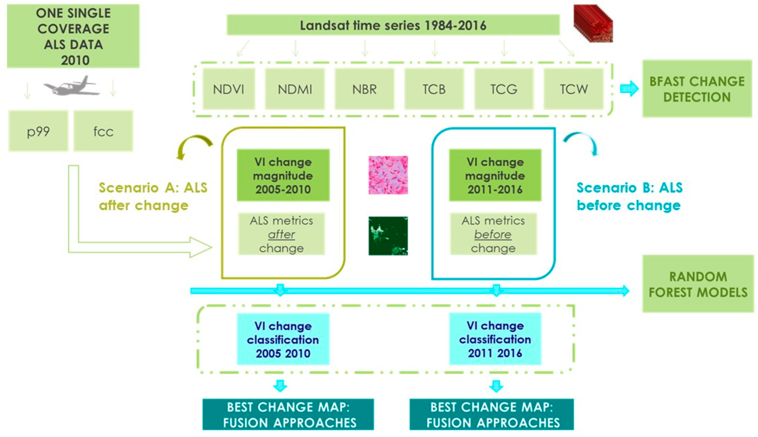
Landsat-based VIs time series were analyzed with BFAST Monitor method [29] using the bfastSpatial package in R (https://github.com/loicdtx/bfastSpatial, accessed on 30 November 2020) and maps of change were generated. We explored two different scenarios to assess the potential implications of having ALS data after or before the detected changes. These scenarios consisted of the definition of two monitoring periods of the same length (5 years) but with a different temporal location of the ALS data (acquired 2010) relative to the monitoring period. (Figure 2). In scenario A the monitoring period is 2005–2010; in scenario B the monitoring period is 2011–2016. With this design, in scenario A the changes detected are those from 2005 to 2010, and in scenario B the changes detected are those from 2011 to 2016. The historic period was determined automatically using the ROC approach implemented in BFAST [29]. A “harmonic” seasonal single-order model was fitted for each historic period (1984–2004 for scenario A, and 1984–2010 for scenario B). The trend component was omitted as it tends to generate false breakpoints and to inflate change in magnitude values [27].

2.2.3. Selection of Training Points

All pixels included in the forest mask were classified into no change or change related to harvesting practices: clear-cutting, cutting with seed-trees and thinning (Figure 3). These three harvesting practices are characterized by a different proportion of cut down trees: clear-cutting involves the removal of all the trees in a stand, cutting with seed-trees implies preserving a small number of dispersed trees needed for natural regeneration, and thinning is an intermediate harvest in which a variable proportion of trees is removed to reduce the stand density and to enhance the quality and growth of the remaining trees. The thinning class included a range of cutting intensities in the area, from light (15%) to heavy (60%) thinning. We did not consider potential subtle changes associated with sanitary issues during the studied period as they were not relevant according to our knowledge of the study area. Reference polygons of variable size (0.3–9.4 ha) were manually digitized based on contemporaneous high-resolution imagery from Google Earth and PNOA (with imagery available from 2005, 2007, 2009, 2011, 2014 and 2017). From each polygon sample points were randomly selected, making up a 400 training samples (100 points per class). The reason behind the decision to create 100 samples per class was to ensure class balance avoiding overestimation of the most representative classes ([57]) and to ensure a large number to accommodate the data dimensions ([58]).

2.3. Classification Models

2.3.1. Random Forests Models

Random Forest (RF) classification models were calibrated with the training sample of 400 points described in Section 2.2.3. An individual RF classification model was fitted for each VI analyzed and each scenario (i.e., six RF models per scenario). ALS metrics (fcc and p99) calculated in Section 2.1.1 as well as the change magnitude derived from BFAST (Section 2.2.2) were used as predictor variables for the calibration of the RF models (Figure 4). In addition to the twelve change maps generated from this classification process (six change maps per scenario), an overall classification model (hereafter called ALL) per scenario was calibrated by employing the ALS metrics and the six VI pools of change magnitudes. Therefore, finally there were a total of 14 change maps. Because RF classifiers consist of a combination of decision trees, where each tree contributes with a prediction and the final class is the most voted by all the decision trees [54], a reliability measure was defined using the percentage of votes (see Section 2.4).
The BFAST output breakpoint timing was not included as a predictor variable for two reasons: (1) it does just marginally improve the accuracy of the classified maps [59] and (2) its inclusion could incur large omission errors due to the existence of changes not declared as structural breakpoints. There could be subtle changes (as thinning operations) that cause a slight decrease not sufficient to surpass the algorithm threshold that defines a structural breakpoint [60].

2.3.2. Validation

The validation process was designed to identify the overall accuracy of the change detection process, and the confusion among change classes in each scenario, via confusion matrices built at the pixel level. Each change map accuracy was individually assessed with independent validation datasets independent from the data used to develop the classification, avoiding any spatial overlapping between the training and validation datasets. The validation dataset consisted of 496 samples for scenario A and 515 for scenario B, allocated following a probabilistic stratified design. The four classes of change (no-change, clear-cutting, cutting with seed-trees and thinning) served as strata, resulting in 348 random points for no-change areas and 148 within change areas for scenario A, and 370 points for no-change and 145 within change areas for the scenario B. High-resolution imagery from Google Earth and PNOA were used to visualize the validation datasets, which were labeled with the type of change (without change year attribution).

2.4. Fusion Maps

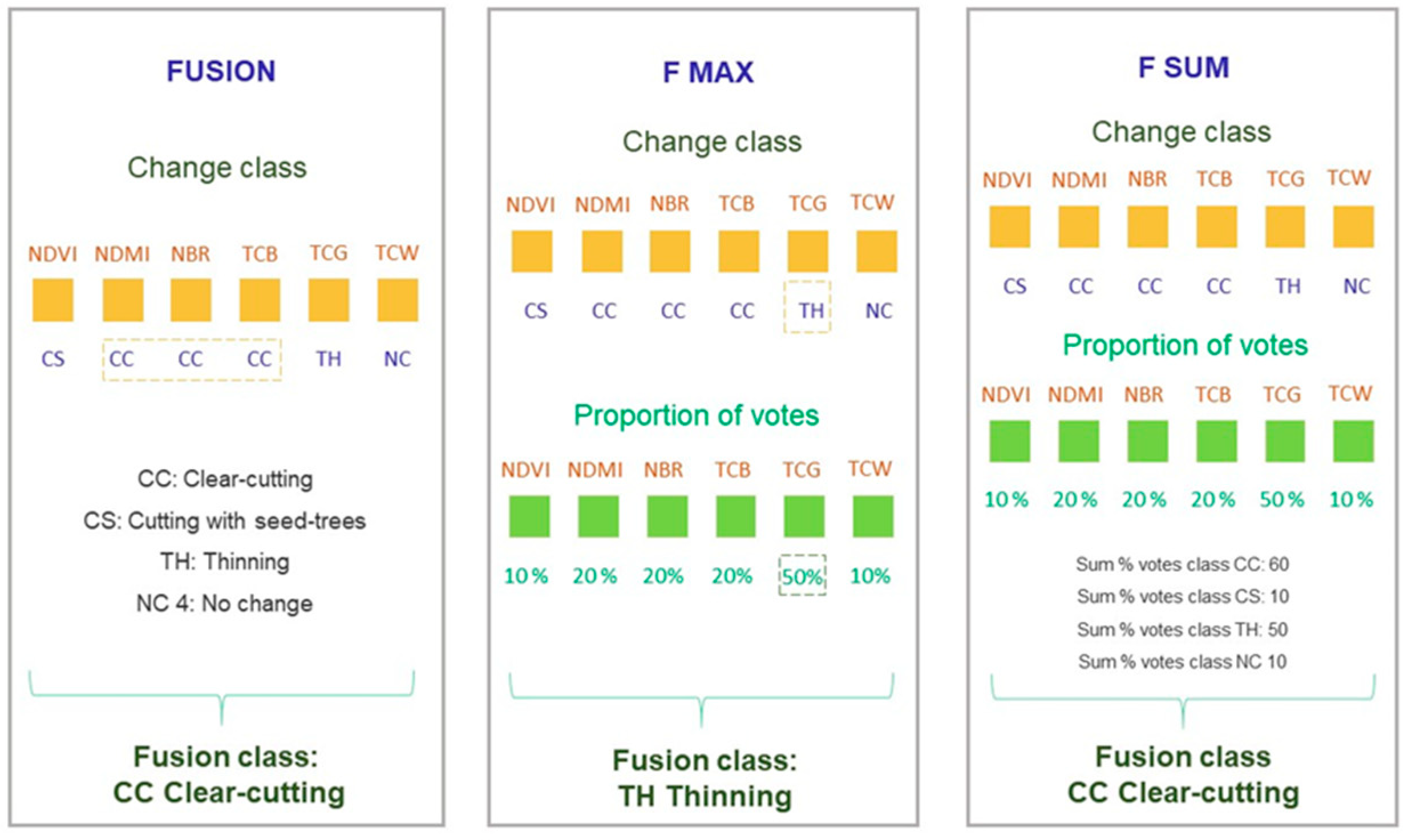
To leverage the potential of each individual VI change map for identification of harvesting practices and to reduce mapping errors [21,28], we created new maps of change by applying three different fusion approaches (Figure 5). Specific rules establishing rankings of frequency and the reliability measure (i.e., percentage of votes in the RF, see Section 2.3.1) of the class assigned in each VI change map were implemented in R code to select fusion classes. When there was a tie in the ranking, the VI change class predicted with the greatest accuracy was preferred. The three fusion techniques implemented are described as follows, where F MAX and F SUM use also the percentage of votes as an aggregation criteria, as in [61]:
(i)
FUSION. A fusion map was created by selecting the most frequent class amongst the six VIs change maps. For example, in Figure 5 clear-cutting is selected, as it happens in 3 out of 6 VI maps;
(ii)
F MAX. A fusion map was created by selecting the class with the greatest reliability measure in any of the VI change maps. For example, in Figure 5 thinning is chosen, since the reliability measure of TCG (50%) is the greatest; and
(iii)
F SUM. A fusion map was created by selecting the overall most voted class, i.e., summing reliability measures of the all VI change maps. For example, in Figure 5 clear-cutting is selected, as the total reliability measure of its three selecting VI (60%) exceeds the reliability measure of the thinning class (50%).

3. Results

3.1. VIs Overall Accuracy Performance

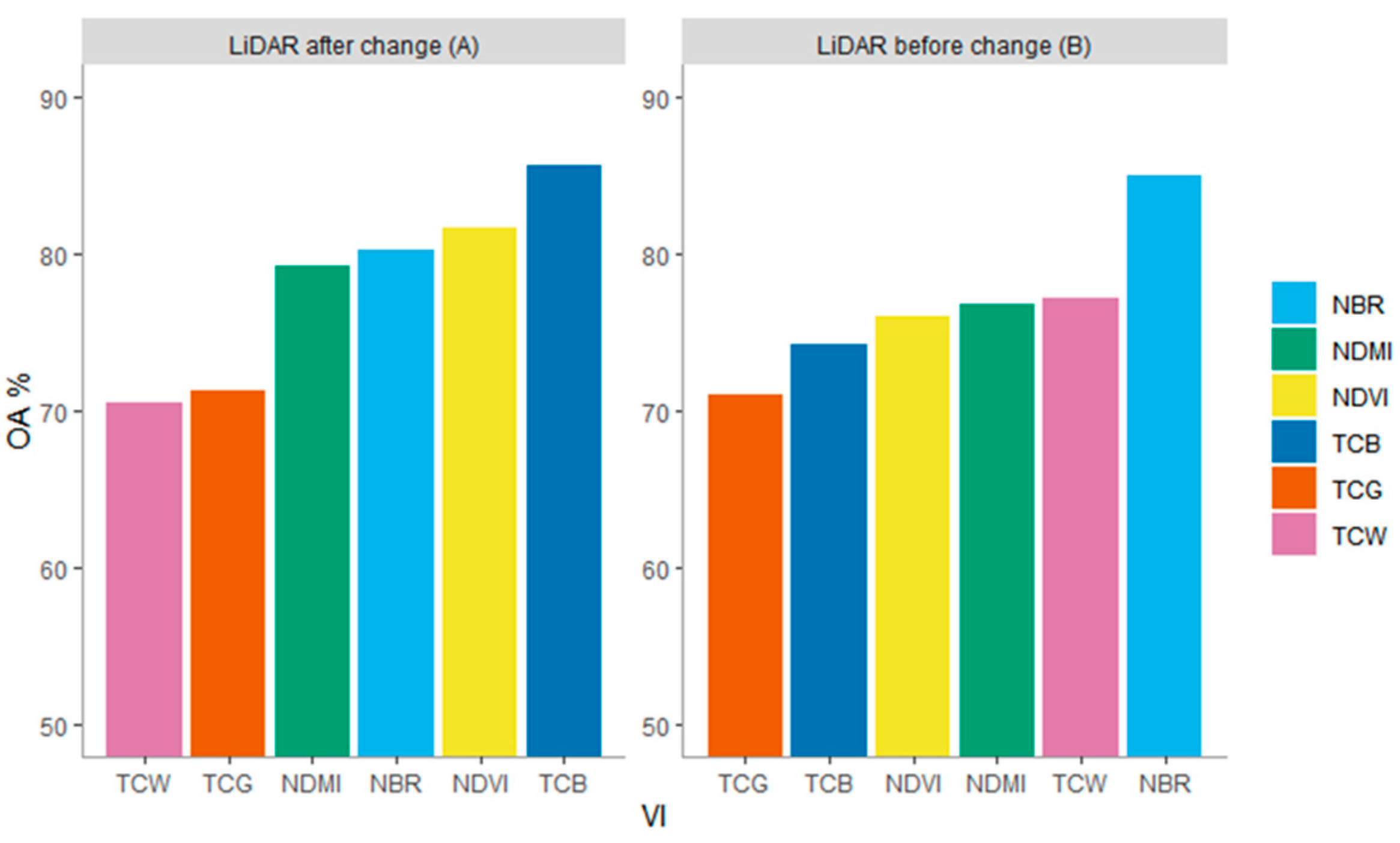
Classifications into the categories no change, clear-cutting, cutting with seed-trees, and thinning, yielded overall accuracies ranging from 70% to 85% (Figure 6). Accuracies were greater for scenario A among the individual VIs tested. TCB and NBR stood out from the rest of the VIs, with overall accuracies over 85%. TCB achieved its best performance (85.69% versus 74.32%) in scenario A (with ALS metrics at the end of the BFAST monitoring period), while NBR improved from 80.24% in scenario A to 85.02% in scenario B (with ALS metrics at the beginning of the BFAST monitoring period). Among the VIs tested, the NDMI and NDVI performed well in both scenarios, showing greater accuracy values for scenario A. The least accurate VI was the TCG with overall accuracy values around 70% and the TCW performed particularly poorly in scenario A (70.56%).

3.2. Performance in Classification of Forestry Practices

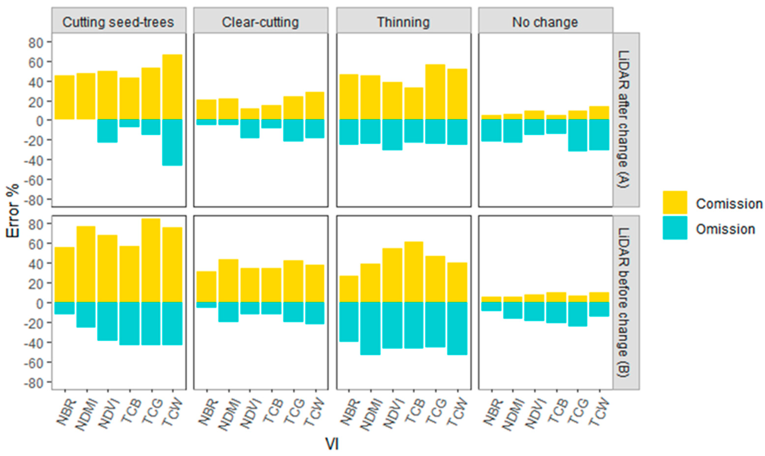
Omission and commission errors differed substantially across harvesting practices with a general increase in errors in scenario B (Figure 7). TCB performed better than the other VIs in identifying the clear-cutting in scenario A, with 15% commission error and 8.11% omission error. However, in scenario B, NBR outperformed TCB, achieving 31.25% and 5.38% of commission and omission errors, respectively. TCB and NBR had similar performance in detecting thinning areas. TCB yielded better results in scenario A, with commission and omission errors of 35.65% and 22.35%, respectively, whereas NBR was the most accurate in scenario B, with commission and omission errors of 40.24% and 26.87%, respectively. As for the cutting with seed-trees class, the NBR was the most accurate VI in both scenarios, with commission and omission errors of 44.68% and 0% in scenario A and 55.56% and 13.04% in scenario B.
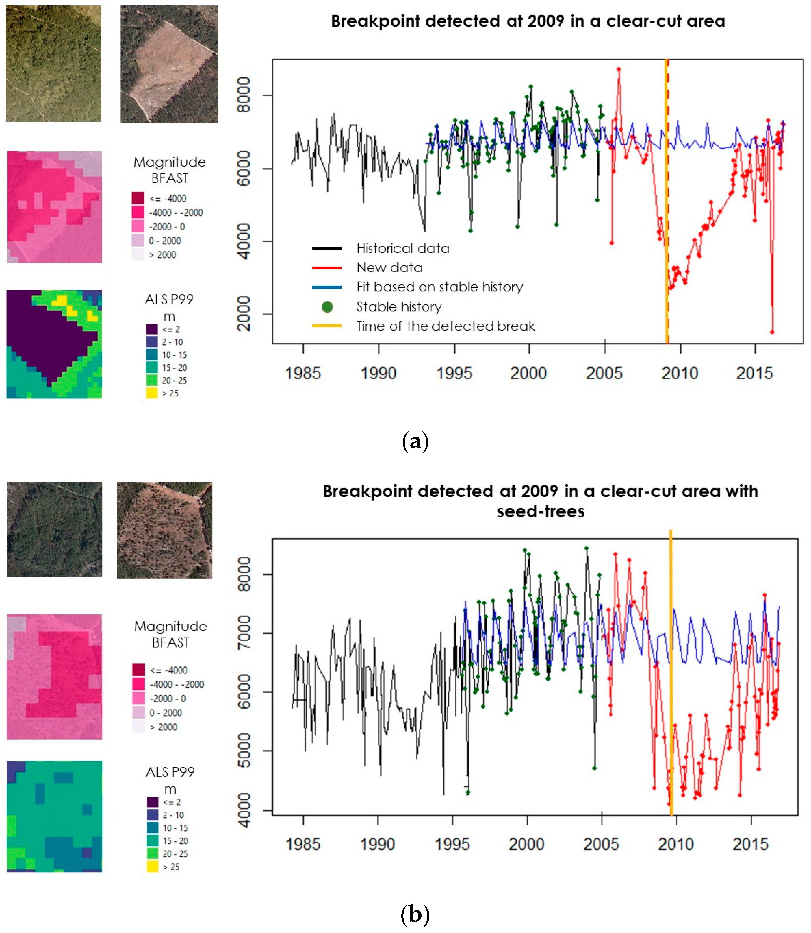
The accuracy assessment revealed that the no-change class had larger omission errors (mostly caused by confusion between non-change and thinning) than commission errors, whereas the other classes were more affected by commission error (Figure 7). The no-change class showed commission and omission errors of 4.75% and 13.51%, respectively, in scenario A, and of 5.37% and 9.46% in scenario B. Clear-cutting was the most accurately classified of the three harvesting practices; in this case, commission errors originated from its confusion with no-change but specially with cutting with seed-trees. Clear-cutting and cutting with seed-trees are expected to produce a similar decrease in the VI magnitude which leads to its misclassification. However, when the cutting-seed tree occurred prior to the ALS acquisition, ALS data detect the trees left for natural regeneration, and contribute to improve their distinction (Figure 8).

3.3. Fusion Maps

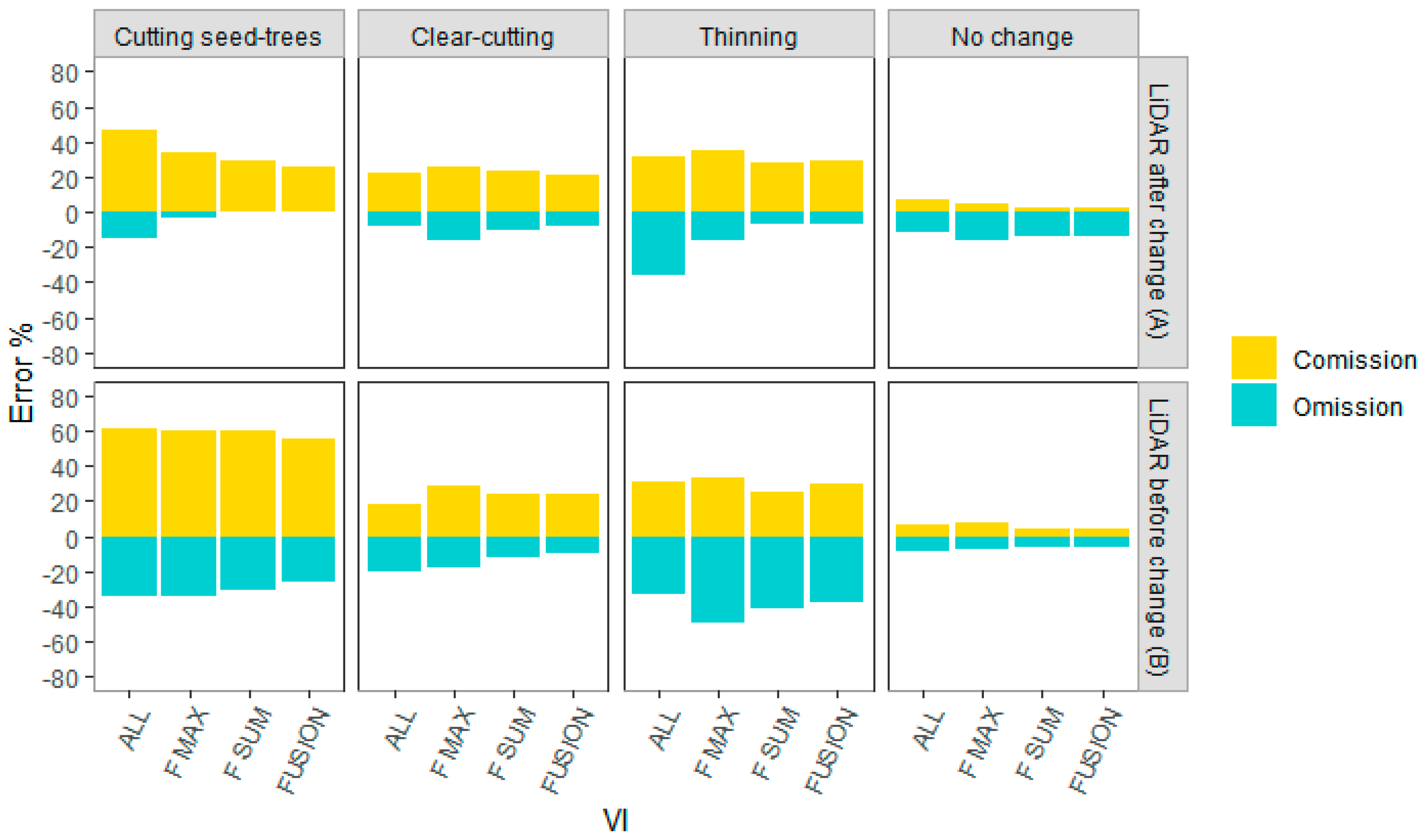
The overall accuracy of the FUSION and FSUM maps were greater than the overall accuracy of FMAX and all individual VI maps. FUSION had an overall accuracy of 88.51% in scenario A and 87.16% in scenario B. Among the three harvesting practices, thinning and cutting with seed-trees benefited more from the fusion approach than clear-cutting (Figure 9). Commission errors of both thinning and cutting with seed-trees were smaller with fusion maps than with any of the VIs individually assessed. For instance, FUSION decreased the commission error of thinning from 35.65% to 28.83% (Table 2) in scenario A (where TCB was the best performing individual VI) and from 40.24% to 29.17% in scenario B (where NBR was the best performing individual VI). The decrease of commission errors in the cutting with seed-trees class is only observed in scenario A (from 44.68% to 25.71%). None of the fusion approaches improved the detection of clear-cutting by individual VIs.

4. Discussion

In this study, we applied methods for identification of forest changes in Mediterranean forests, and classification into three harvesting practices. The TCB and NBR were the most successful VIs among the six essayed [15,16,21,62]. Nevertheless, other VIs like the Normalized Difference Fraction Index (NDFI) and the TCA [63] have shown promising results for detection of changes of low intensity [27,28,64] in other areas and their performance might be tested in our Mediterranean study site.
Clear-cutting was, as expected, the type of change best characterized, with omission and commission errors similar to those achieved by other authors (8.11% and 15% for scenario A and 5.38% and 31.25% for scenario B). Reference [16] reported an omission error of 16.2% for clear-cutting detection in a boreal area in Canada, and clear-cutting was classified in Finland with commission errors ranging between 7–11.6% [18]. Clear-cutting in France was detected with 19% and 54% of omission and commission error, respectively [17], while in Italy, reference [40] achieved omission errors ranging between 16–55% and commission errors smaller than 15%. The similar spectral response caused by clear-cutting and cutting with-seed trees explained in part the commission errors obtained. However, cleared shrublands were also misclassified as clear-cutting, probably due to inaccuracies in the forest mask. It is important to work with an accurate forest mask, to get the best performance from the algorithm [59,60] especially in Mediterranean conditions [40]. Furthermore, the size of Landsat pixels (30 m) makes the derivation of forest masks challenging, particularly in heterogeneous or open forests [28]. The spatial resolution also has an impact on change detection accuracy, particularly for small clear-cut patches [17]. Although a general increase in the harvest patch median size has been observed across Europe [41], Spain shows a median patch size similar to France or Italy, smaller than those observed in northern countries [41].
The low spectral change response that causes thinning operations is more likely to be classified as non-change [16,62], justifying some of the omission errors of this class. Our validation dataset was based on visual interpretation, which may have also impacted the accuracy results of the thinning class. Clear-cutting and intense thinning practices imply a lasting change easily interpreted, while thinning of low intensity might cause canopy openings that rapidly close [65]. Because high-resolution images were only available every two or three years, this temporal resolution might not be sufficient to discern this forestry practice; some of the commission errors could in fact be thinning operations correctly classified by Landsat and BFAST, but misinterpreted in the reference high-resolution images. Reference [66] stated the difficulty to detect non-stand replacing disturbances such as thinning when only annual images were at their disposal. Reference [19] reported that the low thinning intensity that characterized its reference data had a greater effect on the accuracy results as they are more difficult to identify. Besides, our classification scheme did not include subtle disturbances such as insect defoliation or stress and some of these instances could fall into the thinning class [33]. In any case, this approach performance and its accuracy assessment will be better if field points are available as reference [27].
As in [37,62], omission did not exceed commission in the no-change class, being consistent among the VIs analyzed, and proving that it is possible to accurately characterize the forest areas in which no harvesting practices were conducted. The interest of this identification is in connection with ALS-based forest estimates. Even though ALS data benefits have been well-documented [7,67], there is an important handicap related to their temporal resolution. ALS practical usefulness might be reduced in areas where changes happened after data acquisition [68]. Therefore, it is important to identify the unchanged areas in which ALS data continue to be operational, and to assess the use of other metrics to predict current forest attributes in the areas where harvesting practices were conducted [69,70].
The accuracy results obtained for cutting with seed-trees and thinning with individual VI were lower than the results reported in [16] and suggested the convenience to apply fusion techniques to increase accuracy. Among the fusion techniques applied, the three approaches achieved similar accuracy results, albeit slightly greater for the FUSION approach in which percentage of votes is not considered. Further research is recommended to assess the importance of this criterion when fusing methods are applied. Reference [71] applied the fusion techniques based on the percentage of votes to create a forest land cover map, and achieved higher accuracies, but they did not test our FUSION approach.
ALS-derived metrics complement the magnitude metric derived from BFAST by improving the identification of harvesting practices especially when ALS data are acquired after the detected change. The integration of ALS data and Landsat time series enables one to better differentiate those harvesting practices more likely to cause a similar spectral response. Thanks to the increased availability of multi-temporal, wall-to-wall ALS data, in some countries like Spain, an integration of data from different sensors may provide a suitable alternative for detecting harvesting practices more accurately. In the absence of ALS data acquired after the change, RADAR data may be a valuable source of information to discern these forest harvesting practices thanks to its capacity to estimate forest height [72].
Change intensity and ALS metrics were the only predictor variables considered to determine the agent of change. Further work is recommended to fit classification models with change persistence and post-disturbance regrowth [16,73,74] as predictor variables, aiming to better discriminate the forest harvesting practices. In this sense, the potential of using bitemporal ALS data for forest harvesting classification has also been demonstrated [3]. The Spanish second complete ALS coverage is expected to be ready by the end of 2021; these data could also be incorporated for classification purposes. Finally, given the benefits derived from the fusion approaches, different VI synergies should be explored to assess the best VI combination to create more accurate change maps [28].
Our results demonstrate that intense changes such as clear-cuts can be mapped altogether with the same accuracy regardless of the ALS data acquisition date (Figure 7). Hence, Landsat time series can be used solely for drastic change detection when distinguishing between clear-cutting and cutting with seed-trees is not required. In this regard, since the spectral response caused by these changes lasts several years [66], the use of inter-annual time series could be an alternative [75]. Nevertheless, caution should be exercised when considering inter-annual time series since the spectral signal recovery may vary depending on the forest conditions. Clear cuts in Mediterranean forests have shown faster recovery times than clear cuts in boreal forests [15]. Unlike drastic change detection, subtle changes caused by thinning are better characterized with intra-annual time series [18]; thus, time-series algorithms with one image per year frequency are not adequate for thinning detection [31]. Dense time series integrating images from different sensors [76] pose an opportunity to increase the accuracy of the detected changes [23]. Additionally, the BFAST monitoring algorithm has been recently implemented in the Google Earth Engine, supporting the replication of the methodology over large areas and alleviating the users from downloading and processing bulky files [77].
The results obtained in this study confirmed the suitability of integrating one ALS coverage, Landsat time series and BFAST to detect a range of harvesting practices in a Mediterranean study region. Since information about harvesting is important for carbon cycling reports [78], the methodology developed in this work could be implemented to produce annual cartography of harvesting practices enabling more accurate statistics and spatially explicit identification of these operations. Complete and updated national scale cartography of harvesting practices is currently missing, as it is not produced for the study area nor at a national scale [15,79]. Besides, the results obtained can be used in the future to develop and adapt forestry management policies to ensure sustainable management of exploited forest areas [80,81].

5. Conclusions

In this study, six Landsat-based VIs time series were analyzed with the BFAST algorithm, as a means for characterizing changes resulting from harvesting practices of different intensities in a Mediterranean forest area. Fusion approaches were assessed and ALS metrics were included as predictor variables to improve the change characterization. The results demonstrated the suitability of Landsat time series and ALS data to detect changes caused by harvesting practices of different intensity, but with greater accuracy when ALS data were acquired after the change occurred. TCB and NBR were the VIs with better performance, while TCG performed the worst and NBR performed particularly well for thinning classification. Clear-cuttings are more readily detectable compared to cutting with seed-trees and thinning, which requires fusion approaches to increase mapping accuracy. The results are relevant for countries that aim at monitoring their forest interventions and reporting harvest area statistics.

Author Contributions

Conceptualization, J.E., A.F.-L., J.L.T. and C.G.; methodology, J.E., A.F.-L., J.L.T. and C.G.; software, J.E.; validation, J.E. and A.F.-L.; formal analysis, J.E., A.F.-L., J.L.T. and C.G.; investigation, data curation, J.E., A.F.-L., J.L.T. and C.G.; writing—original draft preparation, J.E., A.F.-L., J.L.T., C.G. and M.M.; writing—review and editing, J.E., A.F.-L., J.L.T., C.G. and M.M.; visualization, J.E., A.F.-L., J.L.T. and C.G.; supervision, J.E., A.F.-L., J.L.T. and C.G. All authors have read and agreed to the published version of the manuscript.

Funding

This research received no external funding.

Acknowledgments

We acknowledge the Spanish National Geographic Information Centre (CNIG) for providing the ALS data. We show our gratitude for David De Lasala for assisting with visual image interpretation. We also thank David Mateos for assisting with data visualization in R. This research was primarily supported by the European Commission through funding via SME Instrument, to the project FORESTMAP (REF. 858664, Quick and cost-effective integrated web platform for forest inventories), within its task 2.4. (Development of algorithms based on airborne LIDAR).

Conflicts of Interest

The authors declare no conflict of interest.

References

  1. Vogelmann, J.E.; Gallant, A.L.; Shi, H.; Zhu, Z. Perspectives on monitoring gradual change across the continuity of Landsat sensors using time-series data. Remote Sens. Environ. 2016, 185, 258–270. [Google Scholar] [CrossRef] [Green Version]
  2. Wulder, M.A.; Loveland, T.R.; Roy, D.P.; Crawford, C.J.; Masek, J.G.; Woodcock, C.E.; Allen, R.G.; Anderson, M.C.; Belward, A.S.; Cohen, W.B.; et al. Current status of Landsat program, science, and applications. Remote Sens. Environ. 2019, 225, 127–147. [Google Scholar] [CrossRef]
  3. Noordermeer, L.; Økseter, R.; Ole Ørka, H.; Gobakken, T.; Næsset, E.; Bollandsås, O.M. Classifications of forest change by using bitemporal airborne laser scanner data. Remote Sens. 2019, 11, 2145. [Google Scholar] [CrossRef] [Green Version]
  4. Barrett, F.; McRoberts, R.E.; Tomppo, E.; Cienciala, E.; Waser, L.T. A questionnaire-based review of the operational use of remotely sensed data by national forest inventories. Remote Sens. Environ. 2016, 174, 279–289. [Google Scholar] [CrossRef]
  5. McRoberts, R.E.; Tomppo, E.O. Remote sensing support for national forest inventories. Remote Sens. Environ. 2007, 110, 412–419. [Google Scholar] [CrossRef]
  6. Hansen, M.C.; Loveland, T.R. A review of large area monitoring of land cover change using Landsat data. Remote Sens. Environ. 2012, 122, 66–74. [Google Scholar] [CrossRef]
  7. White, J.C.; Coops, N.C.; Wulder, M.A.; Vastaranta, M.; Hilker, T.; Tompalski, P. Remote Sensing Technologies for Enhancing Forest Inventories: A Review. Can. J. Remote Sens. 2016, 42, 619–641. [Google Scholar] [CrossRef] [Green Version]
  8. Banskota, A.; Kayastha, N.; Falkowski, M.J.; Wulder, M.A.; Froese, R.E.; White, J.C. Forest Monitoring Using Landsat Time Series Data: A Review. Can. J. Remote Sens. 2014, 40, 362–384. [Google Scholar] [CrossRef]
  9. Gómez, C.; White, J.C.; Wulder, M.A. Optical remotely sensed time series data for land cover classification: A review. ISPRS J. Photogramm. Remote Sens. 2016, 116, 55–72. [Google Scholar] [CrossRef] [Green Version]
  10. Wulder, M.A.; White, J.C.; Nelson, R.F.; Næsset, E.; Ørka, H.O.; Coops, N.C.; Hilker, T.; Bater, C.W.; Gobakken, T. Lidar sampling for large-area forest characterization: A review. Remote Sens. Environ. 2012, 121, 196–209. [Google Scholar] [CrossRef] [Green Version]
  11. Woodcock, C.E.; Loveland, T.R.; Herold, M.; Bauer, M.E. Transitioning from change detection to monitoring with remote sensing: A paradigm shift. Remote Sens. Environ. 2019, 238, 111558. [Google Scholar] [CrossRef]
  12. Zhu, Z. Change detection using landsat time series: A review of frequencies, preprocessing, algorithms, and applications. ISPRS J. Photogramm. Remote Sens. 2017, 130, 370–384. [Google Scholar] [CrossRef]
  13. Olsson, H. A method for using Landsat time series for monitoring young plantations in boreal forests. Int. J. Remote Sens. 2009, 30, 5117–5131. [Google Scholar] [CrossRef]
  14. Pflugmacher, D.; Cohen, W.B.; Kennedy, R.E. Using Landsat-derived disturbance history (1972–2010) to predict current forest structure. Remote Sens. Environ. 2012, 122, 146–165. [Google Scholar] [CrossRef]
  15. Chirici, G.; Giannetti, F.; Mazza, E.; Francini, S.; Travaglini, D.; Pegna, R.; White, J.C. Monitoring clearcutting and subsequent rapid recovery in Mediterranean coppice forests with Landsat time series satellite images. Ann. For. Sci. 2020, 77, 40. [Google Scholar] [CrossRef]
  16. Jarron, L.R.; Hermosilla, T.; Coops, N.C.; Wulder, M.A.; White, J.C.; Hobart, G.W.; Leckie, D.G. Differentiation of alternate harvesting practices using annual time series of landsat data. Forests 2017, 8, 15. [Google Scholar] [CrossRef] [Green Version]
  17. Lambert, J.; Denux, J.P.; Verbesselt, J.; Balent, G.; Cheret, V. Detecting clear-cuts and decreases in forest vitality using MODIS NDVI time series. Remote Sens. 2015, 7, 3588–3612. [Google Scholar] [CrossRef] [Green Version]
  18. Pitkänen, T.P.; Sirro, L.; Häme, L.; Häme, T.; Törmä, M.; Kangas, A. Errors related to the automatized satellite-based change detection of boreal forests in Finland. Int. J. Appl. Earth Obs. Geoinf. 2020, 86, 102011. [Google Scholar] [CrossRef]
  19. Ali-Sisto, D.; Packalen, P. Forest Change Detection by Using Point Clouds from Dense Image Matching Together with a LiDAR-Derived Terrain Model. IEEE J. Sel. Top. Appl. Earth Obs. Remote Sens. 2017, 10, 1197–1206. [Google Scholar] [CrossRef]
  20. Arumäe, T.; Lang, M.; Laarmann, D. Thinning- and tree-growth-caused changes in canopy cover and stand height and their estimation using low-density bitemporal airborne lidar measurements—A case study in hemi-boreal forests. Eur. J. Remote Sens. 2020, 53, 113–123. [Google Scholar] [CrossRef] [Green Version]
  21. Cohen, W.B.; Yang, Z.; Healey, S.P.; Kennedy, R.E.; Gorelick, N. A LandTrendr multispectral ensemble for forest disturbance detection. Remote Sens. Environ. 2018, 205, 131–140. [Google Scholar] [CrossRef]
  22. Grogan, K.; Pflugmacher, D.; Hostert, P.; Verbesselt, J.; Fensholt, R. Mapping clearances in tropical dry forests using breakpoints, trend, and seasonal components from modis time series: Does forest type matter? Remote Sens. 2016, 8, 657. [Google Scholar] [CrossRef] [Green Version]
  23. Smith, V.; Portillo-Quintero, C.; Sanchez-Azofeifa, A.; Hernandez-Stefanoni, J.L. Assessing the accuracy of detected breaks in Landsat time series as predictors of small scale deforestation in tropical dry forests of Mexico and Costa Rica. Remote Sens. Environ. 2019, 221, 707–721. [Google Scholar] [CrossRef]
  24. Kennedy, R.E.; Yang, Z.; Cohen, W.B. Detecting trends in forest disturbance and recovery using yearly Landsat time series: 1. LandTrendr—Temporal segmentation algorithms. Remote Sens. Environ. 2010, 114, 2897–2910. [Google Scholar] [CrossRef]
  25. Huang, C.; Goward, S.N.; Masek, J.G.; Thomas, N.; Zhu, Z.; Vogelmann, J.E. An automated approach for reconstructing recent forest disturbance history using dense Landsat time series stacks. Remote Sens. Environ. 2010, 114, 183–198. [Google Scholar] [CrossRef]
  26. Verbesselt, J.; Hyndman, R.; Newnham, G.; Culvenor, D. Detecting trend and seasonal changes in satellite images time series. Remote Sens. Environ. 2010, 114, 106–115. [Google Scholar] [CrossRef]
  27. DeVries, B.; Verbesselt, J.; Kooistra, L.; Herold, M. Robust monitoring of small-scale forest disturbances in a tropical montane forest using Landsat time series. Remote Sens. Environ. 2015, 161, 107–121. [Google Scholar] [CrossRef]
  28. Schultz, M.; Clevers, J.G.P.W.; Carter, S.; Verbesselt, J.; Avitabile, V.; Quang, H.V.; Herold, M. Performance of vegetation indices from Landsat time series in deforestation monitoring. Int. J. Appl. Earth Obs. Geoinf. 2016, 52, 318–327. [Google Scholar] [CrossRef]
  29. Verbesselt, J.; Zeileis, A.; Herold, M. Near real-time disturbance detection using satellite image time series: Drought detection in Somalia. Remote Sens. Environ. 2012, 123, 98–108. [Google Scholar] [CrossRef]
  30. Watts, L.M.; Laffan, S.W. Effectiveness of the BFAST algorithm for detecting vegetation response patterns in a semi-arid region. Remote Sens. Environ. 2014, 154, 234–245. [Google Scholar] [CrossRef]
  31. Wu, L.; Li, Z.; Liu, X.; Zhu, L.; Tang, Y.; Zhang, B.; Xu, B.; Liu, M.; Meng, Y.; Liu, B. Multi-type forest change detection using BFAST and monthly landsat time series for monitoring spatiotemporal dynamics of forests in subtropical wetland. Remote Sens. 2020, 12, 341. [Google Scholar] [CrossRef] [Green Version]
  32. Schmidt, M.; Lucas, R.; Bunting, P.; Verbesselt, J.; Armston, J. Multi-resolution time series imagery for forest disturbance and regrowth monitoring in Queensland, Australia. Remote Sens. Environ. 2015, 158, 156–168. [Google Scholar] [CrossRef] [Green Version]
  33. Fang, X.; Zhu, Q.; Ren, L.; Chen, H.; Wang, K.; Peng, C. Large-scale detection of vegetation dynamics and their potential drivers using MODIS images and BFAST: A case study in Quebec, Canada. Remote Sens. Environ. 2018, 206, 391–402. [Google Scholar] [CrossRef]
  34. Geng, L.; Che, T.; Wang, X.; Wang, H. Detecting spatiotemporal changes in vegetation with the BFAST model in the Qilian Mountain region during 2000–2017. Remote Sens. 2019, 11, 103. [Google Scholar] [CrossRef] [Green Version]
  35. Jin, S.; Yang, L.; Danielson, P.; Homer, C.; Fry, J.; Xian, G. A comprehensive change detection method for updating the National Land Cover Database to circa 2011. Remote Sens. Environ. 2013, 132, 159–175. [Google Scholar] [CrossRef] [Green Version]
  36. Hermosilla, T.; Wulder, M.A.; White, J.C.; Coops, N.C.; Hobart, G.W. Regional detection, characterization, and attribution of annual forest change from 1984 to 2012 using Landsat-derived time-series metrics. Remote Sens. Environ. 2015, 170, 121–132. [Google Scholar] [CrossRef]
  37. Obata, S.; Bettinger, P.; Cieszewski, C.J.; Lowe, R.C. Mapping forest disturbances between 1987–2016 using all available time series landsat TM/ETM+ imagery: Developing a reliable methodology for Georgia, United States. Forests 2020, 11, 335. [Google Scholar] [CrossRef] [Green Version]
  38. Fortin, J.A.; Cardille, J.A.; Perez, E. Multi-sensor detection of forest-cover change across 45 years in Mato Grosso, Brazil. Remote Sens. Environ. 2019, 238, 111266. [Google Scholar] [CrossRef]
  39. Chirici, G.; Giuliarelli, D.; Biscontini, D.; Tonti, D.; Mattioli, W.; Marchetti, M.; Corona, P. Large-scale monitoring of coppice forest clearcuts by multitemporal very high resolution satellite imagery. A case study from central Italy. Remote Sens. Environ. 2011, 115, 1025–1033. [Google Scholar] [CrossRef] [Green Version]
  40. Giannetti, F.; Pegna, R.; Francini, S.; McRoberts, R.E.; Travaglini, D.; Marchetti, M.; Mugnozza, G.S.; Chirici, G. A new method for automated clearcut disturbance detection in mediterranean coppice forests using landsat time series. Remote Sens. 2020, 12, 3720. [Google Scholar] [CrossRef]
  41. Ceccherini, G.; Duveiller, G.; Grassi, G.; Lemoine, G.; Avitabile, V.; Pilli, R.; Cescatti, A. Abrupt increase in harvested forest area over Europe after 2015. Nature 2020, 583, 72–77. [Google Scholar] [CrossRef]
  42. McRae, D.J.; Duchesne, L.C.; Freedman, B.; Lynham, T.J.; Woodley, S. Comparisons between wildfire and forest harvesting and their implications in forest management. Environ. Rev. 2001, 9, 223–260. [Google Scholar] [CrossRef]
  43. Segur, M. Los bosques modelo y el bosque modelo Urbión. Rev. Montes 2009, 98, 96–99. [Google Scholar]
  44. González-Olabarria, J.R.; Rodríguez, F.; Fernández-Landa, A.; Mola-Yudego, B. Mapping fire risk in the Model Forest of Urbión (Spain) based on airborne LiDAR measurements. For. Ecol. Manag. 2012, 282, 149–156. [Google Scholar] [CrossRef]
  45. PNOA Spanish National Program of Aerial Orthophotography (PNOA). Available online: http://pnoa.ign.es/presentacion (accessed on 30 November 2020).
  46. McGaughey, R.; Forester, R.; Carson, W. Fusing LIDAR data, photographs, and other data using 2D and 3D visualization techniques. Proc. Terrain Data Appl. Vis. Connect. 2003, 28–30, 16–24. [Google Scholar]
  47. Zhu, Z.; Wang, S.; Woodcock, C.E. Improvement and expansion of the Fmask algorithm: Cloud, cloud shadow, and snow detection for Landsats 4–7, 8, and Sentinel 2 images. Remote Sens. Environ. 2015, 159, 269–277. [Google Scholar] [CrossRef]
  48. Rouse, J.W.J.; Haas, R.; Schell, J.; Deering, D. Monitoring Vegetation System in the Great Plains with ETRS. In Proceedings of the Third Earth Resources Technology Satellite-1 Symposium, Greenbelt, MD, USA; 1974; pp. 309–317. Available online: https://ntrs.nasa.gov/api/citations/19740022614/downloads/19740022614.pdf (accessed on 8 September 2021).
  49. Hunt, E.R.; Rock, B.N. Detection of changes in leaf water content using Near- and Middle-Infrared reflectances. Remote Sens. Environ. 1989, 30, 43–54. [Google Scholar] [CrossRef]
  50. García, M.J.L.; Caselles, V. Mapping burns and natural reforestation using thematic Mapper data. Geocarto Int. 1991, 6, 31–37. [Google Scholar] [CrossRef]
  51. Crist, E.P. A TM Tasseled Cap equivalent transformation for reflectance factor data. Remote Sens. Environ. 1985, 17, 301–306. [Google Scholar] [CrossRef]
  52. Huang, C.; Wylie, B.; Yang, L.; Homer, C.; Zylstra, G. Derivation of a tasselled cap transformation based on Landsat 7 at-satellite reflectance. Int. J. Remote Sens. 2002, 23, 1741–1748. [Google Scholar] [CrossRef]
  53. Baig, M.H.A.; Zhang, L.; Shuai, T.; Tong, Q. Derivation of a tasselled cap transformation based on Landsat 8 at-satellite reflectance. Remote Sens. Lett. 2014, 5, 423–431. [Google Scholar] [CrossRef]
  54. Breiman, L. Random Forests. Mach. Learn. 2001, 45, 5–32. [Google Scholar] [CrossRef] [Green Version]
  55. Liaw, A.; Wiener, M. Classification and Regression by randomForest. R News 2002, 2, 18–22. [Google Scholar] [CrossRef]
  56. Genuer, R.; Poggi, J.-M.; Tuleau-Malot, C. VSURF: An R Package for Variable Selection Using Random Forests. R J. 2015, 7, 19–33. [Google Scholar] [CrossRef] [Green Version]
  57. Dalponte, M.; Bruzzone, L.; Gianelle, D. Tree species classification in the Southern Alps based on the fusion of very high geometrical resolution multispectral/hyperspectral images and LiDAR data. Remote Sens. Environ. 2012, 123, 258–270. [Google Scholar] [CrossRef]
  58. Belgiu, M.; Drăguţ, L. Random forest in remote sensing: A review of applications and future directions. ISPRS J. Photogramm. Remote Sens. 2016, 114, 24–31. [Google Scholar] [CrossRef]
  59. DeVries, B.; Decuyper, M.; Verbesselt, J.; Zeileis, A.; Herold, M.; Joseph, S. Tracking disturbance-regrowth dynamics in tropical forests using structural change detection and Landsat time series. Remote Sens. Environ. 2015, 169, 320–334. [Google Scholar] [CrossRef]
  60. Bullock, E.L.; Woodcock, C.E.; Olofsson, P. Monitoring tropical forest degradation using spectral unmixing and Landsat time series analysis. Remote Sens. Environ. 2018, 238, 110968. [Google Scholar] [CrossRef]
  61. Lewinski, S.; Nowakowski, A.; Rybicki, M.; Kukawska, E.; Malinowski, R.; Krupiński, M. Aggregation of Sentinel-2 time series classifications as a solution for multitemporal analysis. In Proceedings of the SPIE 10427, Image and Signal Processing for Remote Sensing XXIII, Warsaw, Poland, 4 October 2017; p. 11. [Google Scholar]
  62. Huo, L.Z.; Boschetti, L.; Sparks, A.M. Object-based classification of forest disturbance types in the conterminous United States. Remote Sens. 2019, 11, 477. [Google Scholar] [CrossRef] [Green Version]
  63. Powell, S.L.; Cohen, W.B.; Healey, S.P.; Kennedy, R.E.; Moisen, G.G.; Pierce, K.B.; Ohmann, J.L. Quantification of live aboveground forest biomass dynamics with Landsat time-series and field inventory data: A comparison of empirical modeling approaches. Remote Sens. Environ. 2010, 114, 1053–1068. [Google Scholar] [CrossRef]
  64. Gómez, C.; Wulder, M.A.; White, J.C.; Montes, F.; Delgado, J.A. Characterizing 25 years of change in the area, distribution, and carbon stock of Mediterranean pines in Central Spain. Int. J. Remote Sens. 2012, 33, 5546–5573. [Google Scholar] [CrossRef]
  65. Puettmann, K.J.; Ares, A.; Burton, J.I.; Dodson, E.K. Forest Restoration Using Variable Density Thinning: Lessons from Douglas-Fir Stands in Western Oregon. Forests 2016, 7, 310. [Google Scholar] [CrossRef] [Green Version]
  66. Schroeder, T.A.; Wulder, M.A.; Healey, S.P.; Moisen, G.G. Mapping wildfire and clearcut harvest disturbances in boreal forests with Landsat time series data. Remote Sens. Environ. 2011, 115, 1421–1433. [Google Scholar] [CrossRef]
  67. Margolis, H.A.; Nelson, R.F.; Montesano, P.M.; Beaudoin, A.; Sun, G.; Andersen, H.-E.; Wulder, M.A. Combining satellite lidar, airborne lidar, and ground plots to estimate the amount and distribution of aboveground biomass in the boreal forest of North America. Can. J. For. Res. 2015, 45, 838–855. [Google Scholar] [CrossRef] [Green Version]
  68. McRoberts, R.E.; Chen, Q.; Gormanson, D.D.; Walters, B.F. The shelf-life of airborne laser scanning data for enhancing forest inventory inferences. Remote Sens. Environ. 2018, 206, 254–259. [Google Scholar] [CrossRef]
  69. Ahmed, O.S.; Franklin, S.E.; Wulder, M.A.; White, J.C. Characterizing stand-level forest canopy cover and height using Landsat time series, samples of airborne LiDAR, and the Random Forest algorithm. ISPRS J. Photogramm. Remote Sens. 2015, 101, 89–101. [Google Scholar] [CrossRef]
  70. Pflugmacher, D.; Cohen, W.B.; Kennedy, R.E.; Yang, Z. Using Landsat-derived disturbance and recovery history and lidar to map forest biomass dynamics. Remote Sens. Environ. 2014, 151, 124–137. [Google Scholar] [CrossRef]
  71. Alonso, L.; Picos, J.; Armesto, J. Forest Land Cover Mapping at a Regional Scale Using Multi-Temporal Sentinel-2 Imagery and RF Models. Remote Sens. 2021, 13, 2237. [Google Scholar] [CrossRef]
  72. Lei, Y.; Siqueira, P. Estimation of Forest Height Using Spaceborne Repeat-Pass-L-Band InSAR Correlation Magnitude over the US State of Maine. Remote Sens. 2014, 6, 10252–10285. [Google Scholar] [CrossRef] [Green Version]
  73. Coops, N.C.; Shang, C.; Wulder, M.A.; White, J.C.; Hermosilla, T. Change in forest condition: Characterizing non-stand replacing disturbances using time series satellite imagery. For. Ecol. Manag. 2020, 474, 118370. [Google Scholar] [CrossRef]
  74. Hermosilla, T.; Wulder, M.A.; White, J.C.; Coops, N.C. Prevalence of multiple forest disturbances and impact on vegetation regrowth from interannual Landsat time series (1985–2015). Remote Sens. Environ. 2019, 233, 111403. [Google Scholar] [CrossRef]
  75. Saxena, R.; Watson, L.T.; Wynne, R.H.; Brooks, E.B.; Thomas, V.A.; Zhiqiang, Y.; Kennedy, R.E. Towards a polyalgorithm for land use change detection. ISPRS J. Photogramm. Remote Sens. 2018, 144, 217–234. [Google Scholar] [CrossRef]
  76. Claverie, M.; Ju, J.; Masek, J.G.; Dungan, J.L.; Vermote, E.F.; Roger, J.; Skakun, S.V.; Justice, C. The Harmonized Landsat and Sentinel-2 surface reflectance data set. Remote Sens. Environ. 2018, 219, 145–161. [Google Scholar] [CrossRef]
  77. Hamunyela, E.; Rosca, S.; Mirt, A.; Engle, E.; Herold, M.; Gieseke, F.; Verbesselt, J. Implementation of BFASTmonitor Algorithm on Google Earth Engine to Support Large-Area and Sub-Annual Change Monitoring Using Earth Observation Data. Remote Sens. 2020, 12, 2953. [Google Scholar] [CrossRef]
  78. Davis, S.C.; Hessl, A.E.; Scott, C.J.; Adams, M.B.; Thomas, R.B. Forest carbon sequestration changes in response to timber harvest. For. Ecol. Manag. 2009, 258, 2101–2109. [Google Scholar] [CrossRef]
  79. Gomez, C.; Alejandro, P.; Hermosilla, T.; Montes, F.; Pascual, C.; Ruiz, L.Á.; Alvarez-taboada, F.; Tanase, M.A.; Valbuena, R. Remote sensing for the Spanish forests in the 21st century : A review of advances, needs, and opportunities. For. Syst. 2019, 28. [Google Scholar] [CrossRef]
  80. Buhal, T. Detecting Clear-Cut Deforestation Using Landsat Data : A Time Series Analysis of Remote Sensing Data in Covasna County, Romania between 2005 and 2015. Lund University. 2016. Available online: https://lup.lub.lu.se/student-papers/search/publication/8892796 (accessed on 8 September 2021).
  81. Ciobotaru, A.M.; Andronache, I.; Ahammer, H.; Jelinek, H.F.; Radulovic, M.; Pintilii, R.D.; Peptenatu, D.; Draghici, C.C.; Simion, A.G.; Papuc, R.M.; et al. Recent deforestation pattern changes (2000–2017) in the Central Carpathians: A gray-level co-occurrence matrix and fractal analysis approach. Forests 2019, 10, 308. [Google Scholar] [CrossRef] [Green Version]
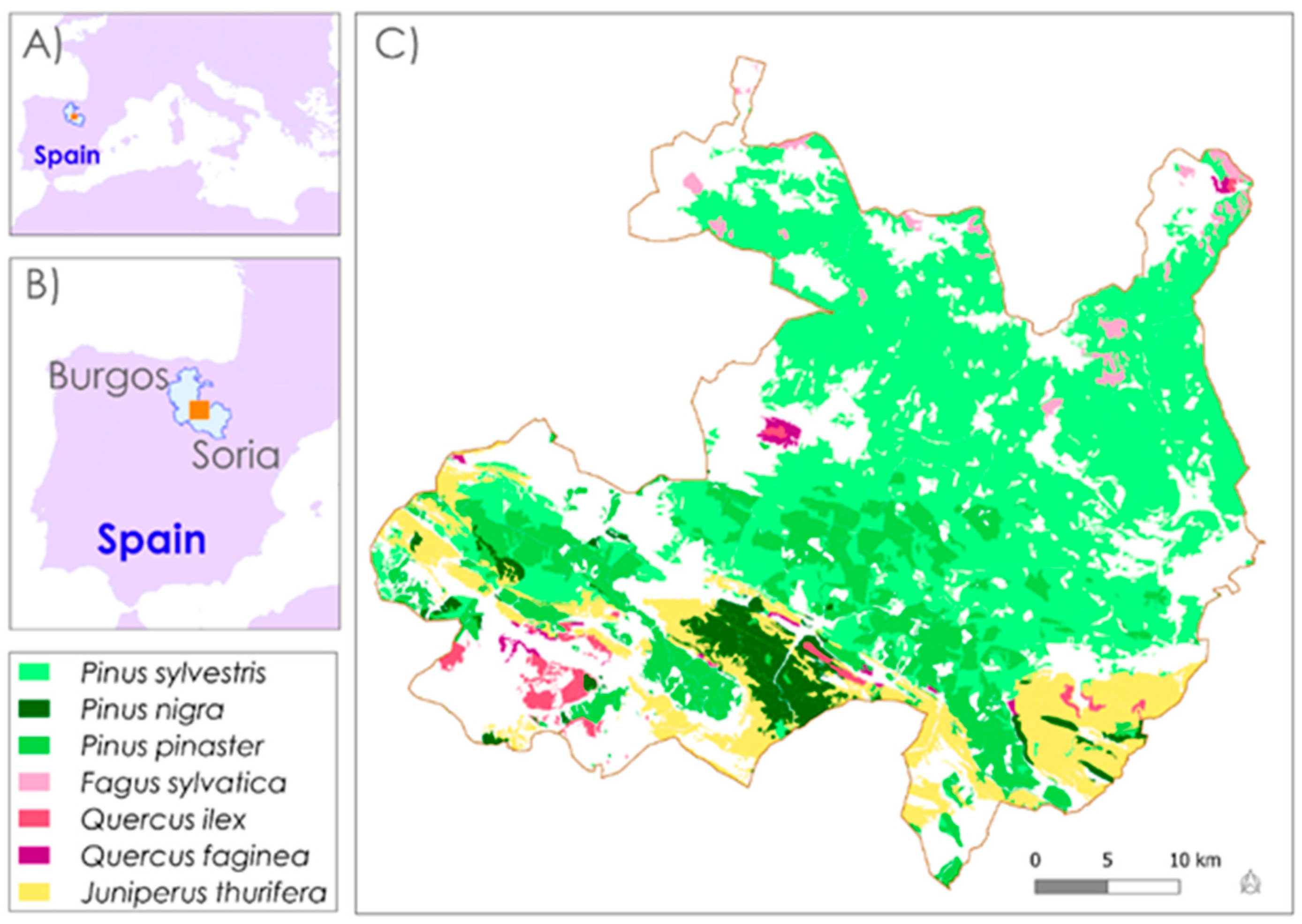
Figure 1. (A) Location of the study area in the Mediterranean basin, in the Spanish provinces of Burgos and Soria (B), and (C) main forest species distribution in the Urbión Model Forest, according to the Spanish National Forest Map.
Remotesensing 13 03611 g001
Figure 2. Number of scenes used per year analyzed with BFAST, and visualization of historic and monitoring periods. Two scenarios are considered to assess how ALS data may help characterizing change. In scenario A, ALS metrics are available at the end of the monitoring period; in scenario B, ALS metrics are available at the beginning of the monitoring period.
Remotesensing 13 03611 g002
Figure 3. Examples of changes related to the harvesting practices (clear-cutting, cutting with seed trees, thinning) identified in this work. Changes are shown with high-resolution imagery before and after the change.
Remotesensing 13 03611 g003
Figure 4. General methodology workflow applied for classification of changes related to forest harvesting practices in scenario A and scenario B.
Remotesensing 13 03611 g004
Figure 5. Example of different fusion options conducted for a specific pixel classified with six RF models, each calibrated with different outputs from the BFAST analysis. The change classes are: (1) clear-cutting (CC), (2) cutting with seed-trees (CS), (3) thinning operations (TH) and (4) no change (NC).
Remotesensing 13 03611 g005
Figure 6. Overall accuracy (OA) results (%) for the detection of different harvesting practices using six VIs (NDVI, NDMI, NBR, TCB, TCG and TCW); (left): scenario A, when ALS data were acquired at the end of the monitoring period; (right): scenario B, when ALS data were acquired at the beginning of the monitoring period.
Remotesensing 13 03611 g006
Figure 7. Validation of the change classification performed in the study area for each monitoring period analyzing different VI time series with the BFAST algorithm. (A): scenario A, when ALS data were acquired at the end of the monitoring period; (B): scenario B, when ALS data were acquired at the beginning of the monitoring period.
Remotesensing 13 03611 g007
Figure 8. NBR BFAST results and ALS P99 metric differences for two pixels in which a breakpoint is detected in 2009. (a) Represents a pixel within a clear-cutting area while (b) is a cutting with-seed trees pixel.
Remotesensing 13 03611 g008
Figure 9. Commission and omission errors of the fusion change classification approaches. (A): Scenario A, when ALS data were acquired at the end of the monitoring period; (B): scenario B, when ALS data were acquired at the beginning of the monitoring period.
Remotesensing 13 03611 g009
Table 1. Vegetation indexes calculated from the Landsat bands, where NIR is the near infrared band and SWIR1 and SWIR2 the first and second shortwave infrared bands, respectively.
Vegetation IndexFormulaReference
NDVI(NIR − RED)/(NIR + RED)[48]
NDMI(NIR − SWIR1)/(NIR + SWIR1)[49]
NBR(NIR − SWIR2)/(NIR + SWIR2)[50]
TCB [51,52,53]
TCG [51,52,53]
TCW [51,52,53]
Table 2. Validation of the best change classifications performed in the study area for each scenario of monitoring period and for the fusion results of all the VIs used in this study. Errors units are %.
Scenario A
Monitoring Period: 2005–2010
ALS after Change
Scenario B
Monitoring Period: 2011–2016
ALS before Change
The most successful VIs: TCBThe most successful VIs: NBR
ClassCommission errorOmission errorCommission errorOmission error
Cutting with seed-trees44.680.0055.5613.04
Clear-cutting15.008.1131.255.38
Thinning35.6522.3540.2426.87
No change4.7513.515.379.46
Fusion approachFusion approach
ClassCommission errorOmission errorCommission errorOmission error
Cutting with seed-trees25.710.0055.2626.09
Clear-cutting20.938.1123.9110.26
Thinning28.837.0629.1737.80
No change2.2813.793.636.76
Publisher’s Note: MDPI stays neutral with regard to jurisdictional claims in published maps and institutional affiliations.