
Identification of Silvicultural Practices in Mediterranean Forests Integrating Landsat Time Series and a Single Coverage of ALS Data

 , ,
, ,  and
and
Abstract
:
1. Introduction
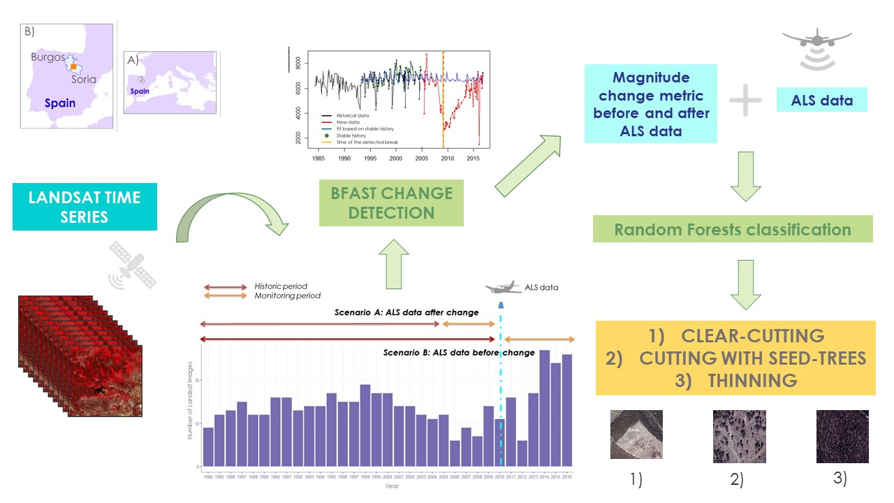
2. Materials and Methods
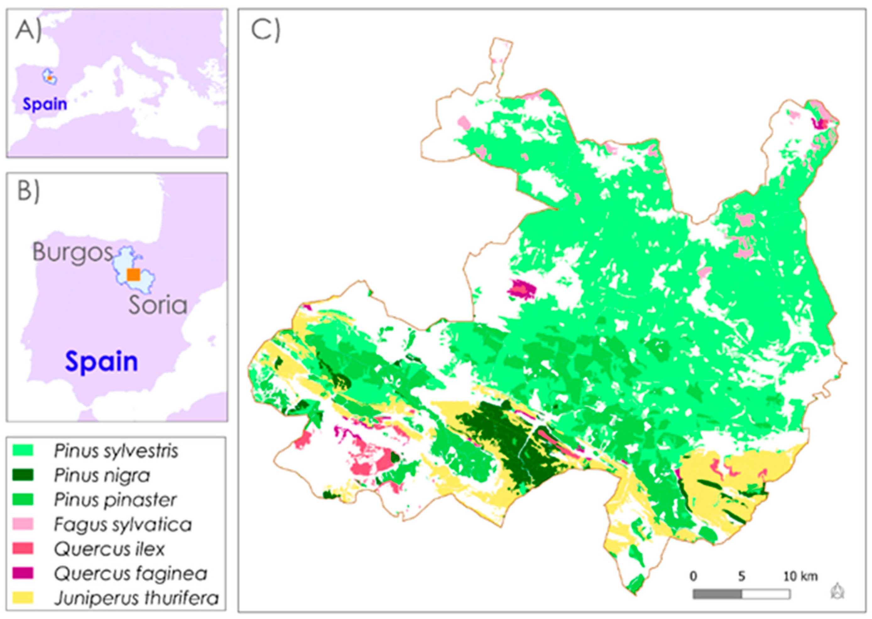
2.1. Study Area and Data
2.1.1. ALS Data
2.1.2. Landsat Time Series
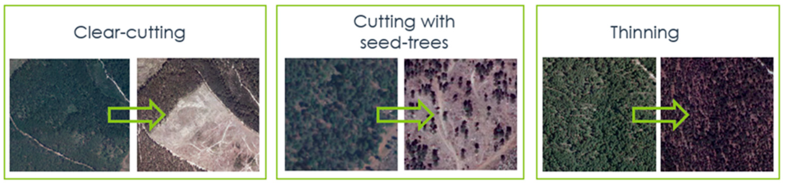
2.2. Detection of Harvesting Practices
2.2.1. Forest Mask
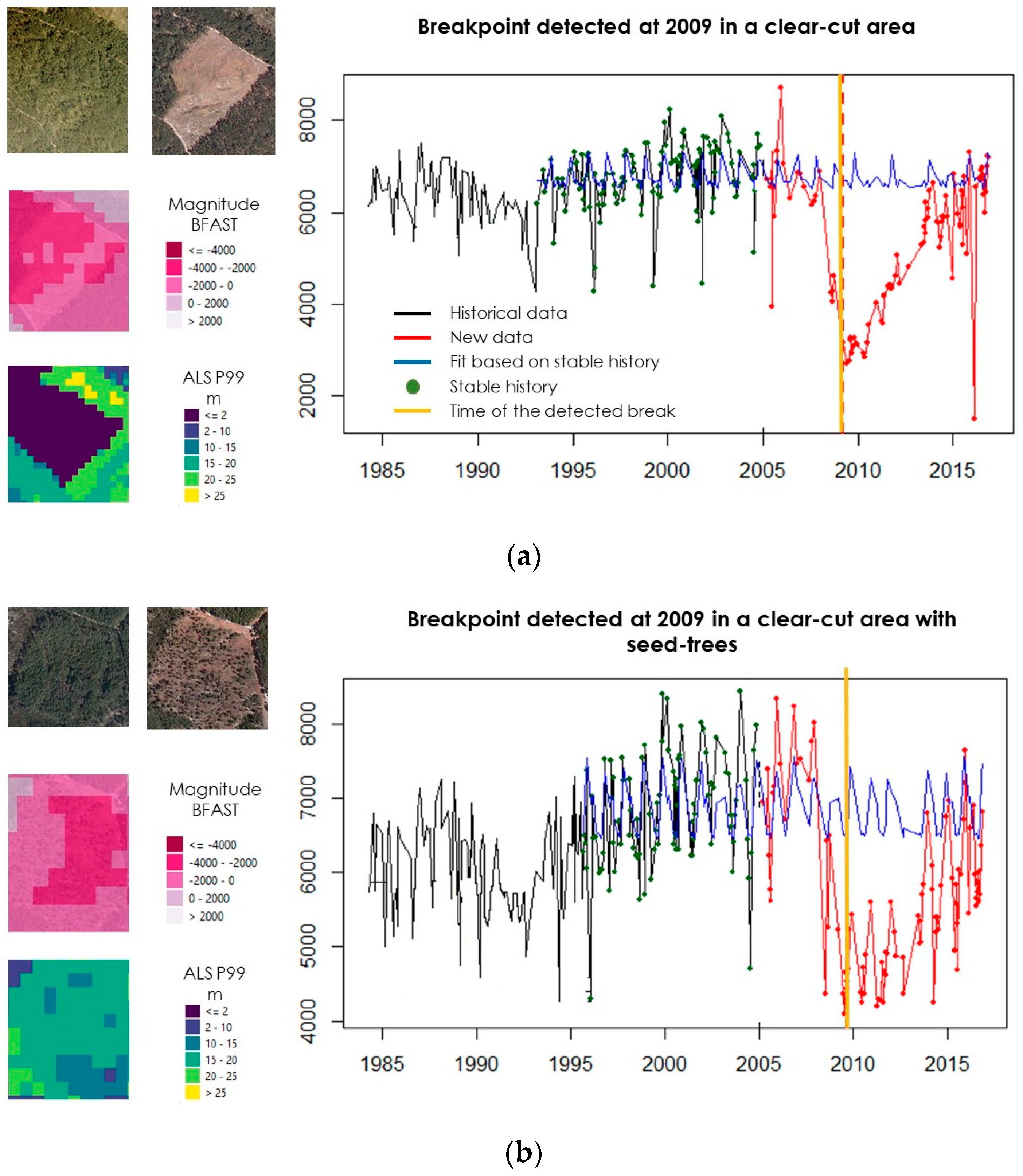
2.2.2. BFAST Implementation
2.2.3. Selection of Training Points
2.3. Classification Models
2.3.1. Random Forests Models
2.3.2. Validation
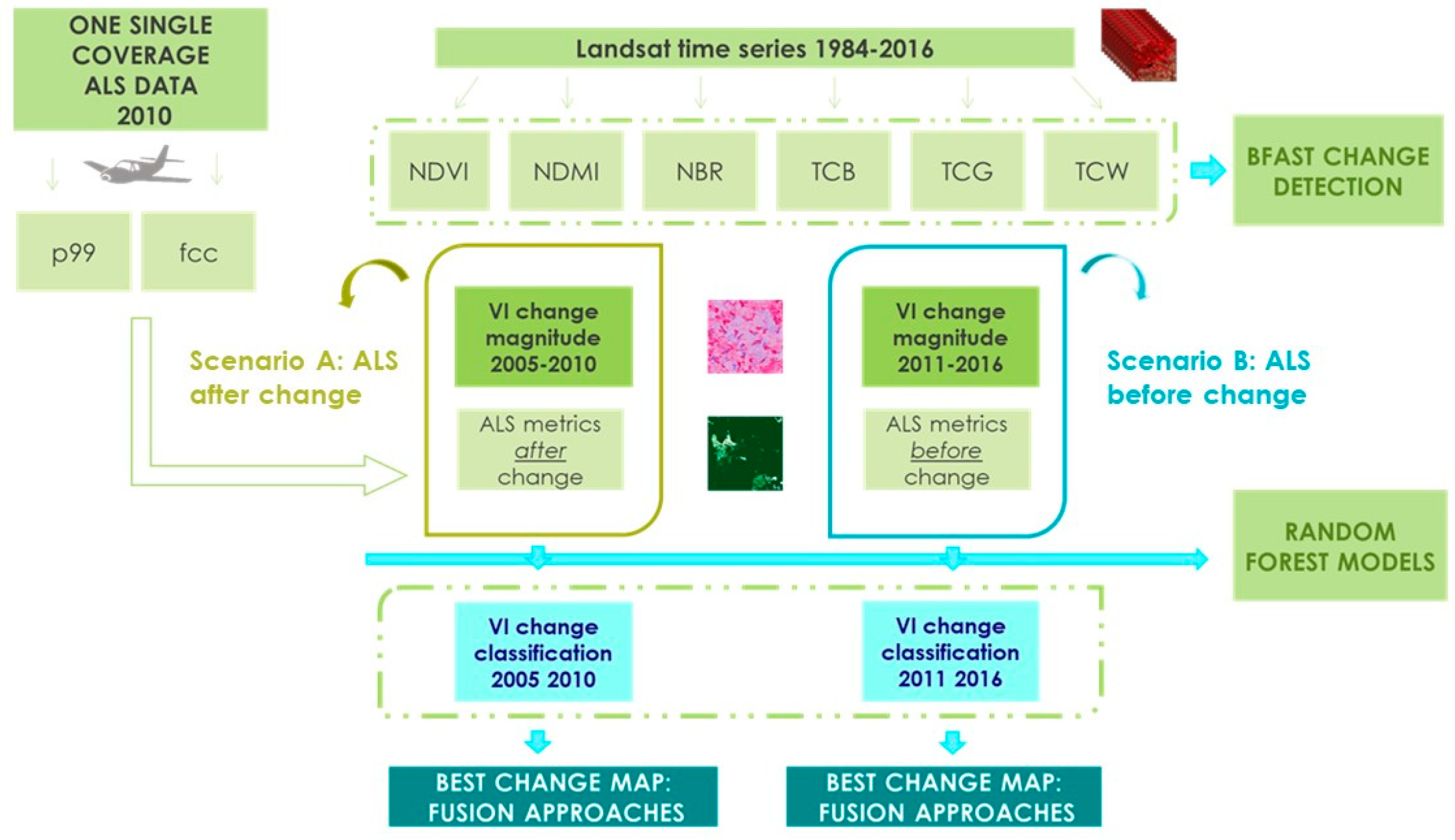
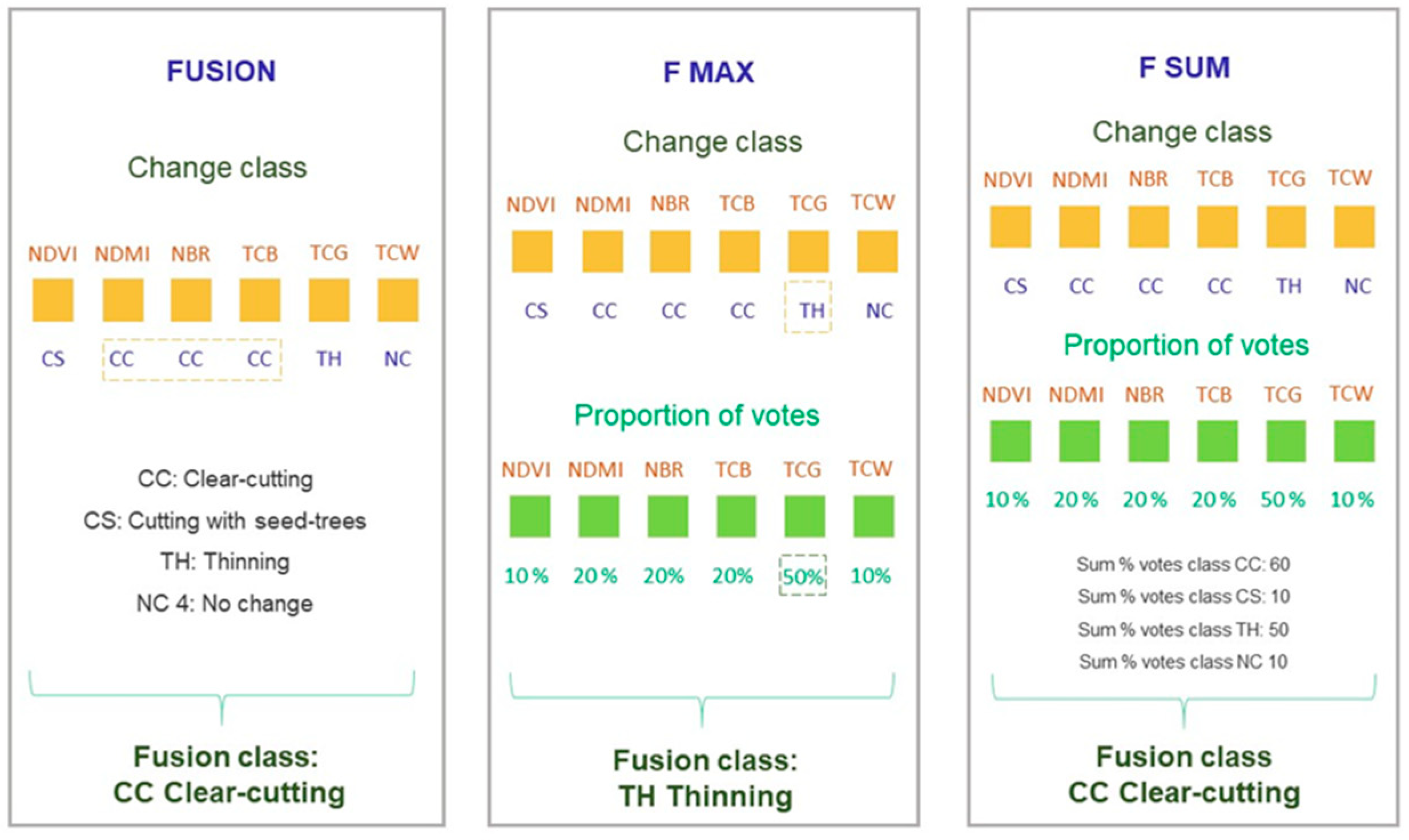
2.4. Fusion Maps
- (i)
- FUSION. A fusion map was created by selecting the most frequent class amongst the six VIs change maps. For example, in Figure 5 clear-cutting is selected, as it happens in 3 out of 6 VI maps;
- (ii)
- F MAX. A fusion map was created by selecting the class with the greatest reliability measure in any of the VI change maps. For example, in Figure 5 thinning is chosen, since the reliability measure of TCG (50%) is the greatest; and
- (iii)
- F SUM. A fusion map was created by selecting the overall most voted class, i.e., summing reliability measures of the all VI change maps. For example, in Figure 5 clear-cutting is selected, as the total reliability measure of its three selecting VI (60%) exceeds the reliability measure of the thinning class (50%).
3. Results
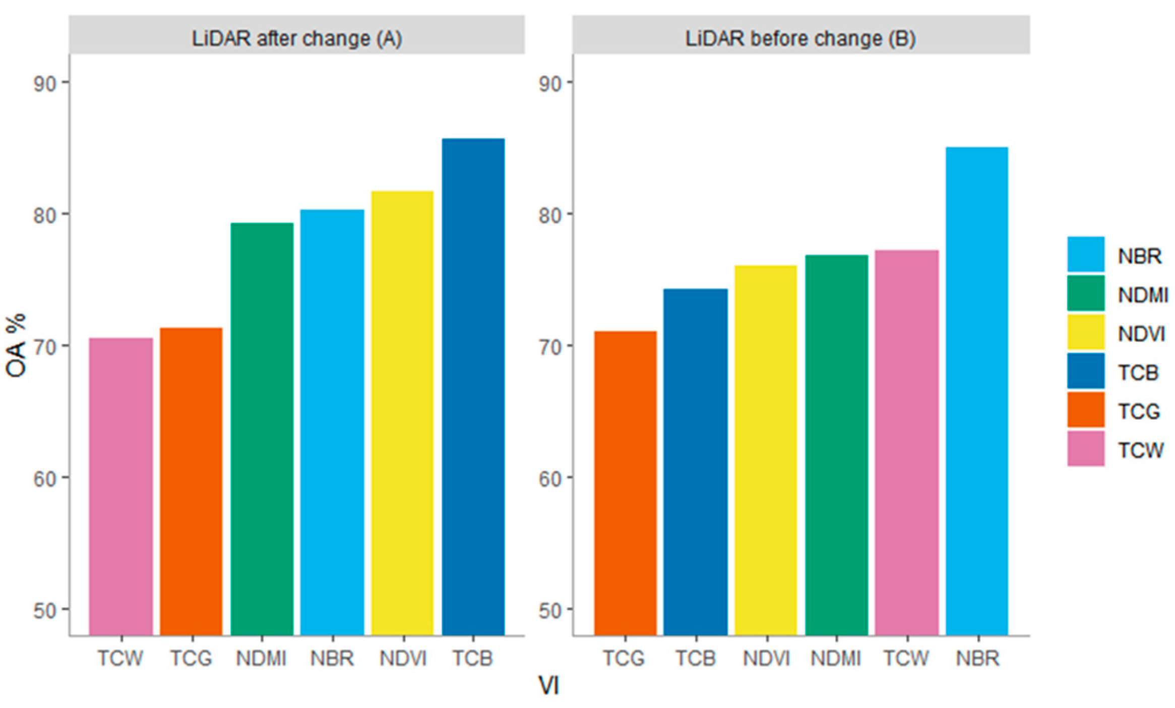
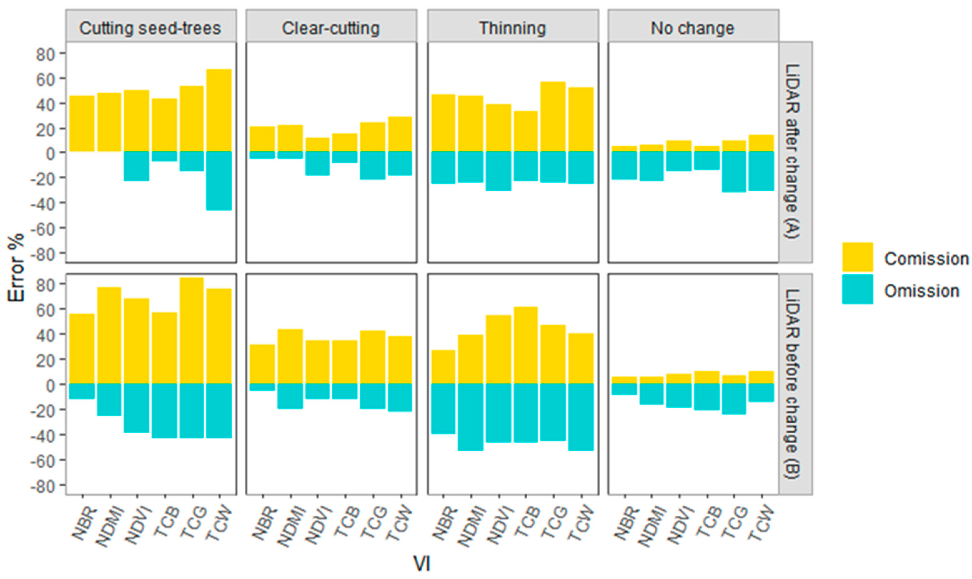
3.1. VIs Overall Accuracy Performance
3.2. Performance in Classification of Forestry Practices
3.3. Fusion Maps
4. Discussion
5. Conclusions
Author Contributions
Funding
Acknowledgments
Conflicts of Interest
References
- Vogelmann, J.E.; Gallant, A.L.; Shi, H.; Zhu, Z. Perspectives on monitoring gradual change across the continuity of Landsat sensors using time-series data. Remote Sens. Environ. 2016, 185, 258–270. [Google Scholar] [CrossRef] [Green Version]
- Wulder, M.A.; Loveland, T.R.; Roy, D.P.; Crawford, C.J.; Masek, J.G.; Woodcock, C.E.; Allen, R.G.; Anderson, M.C.; Belward, A.S.; Cohen, W.B.; et al. Current status of Landsat program, science, and applications. Remote Sens. Environ. 2019, 225, 127–147. [Google Scholar] [CrossRef]
- Noordermeer, L.; Økseter, R.; Ole Ørka, H.; Gobakken, T.; Næsset, E.; Bollandsås, O.M. Classifications of forest change by using bitemporal airborne laser scanner data. Remote Sens. 2019, 11, 2145. [Google Scholar] [CrossRef] [Green Version]
- Barrett, F.; McRoberts, R.E.; Tomppo, E.; Cienciala, E.; Waser, L.T. A questionnaire-based review of the operational use of remotely sensed data by national forest inventories. Remote Sens. Environ. 2016, 174, 279–289. [Google Scholar] [CrossRef]
- McRoberts, R.E.; Tomppo, E.O. Remote sensing support for national forest inventories. Remote Sens. Environ. 2007, 110, 412–419. [Google Scholar] [CrossRef]
- Hansen, M.C.; Loveland, T.R. A review of large area monitoring of land cover change using Landsat data. Remote Sens. Environ. 2012, 122, 66–74. [Google Scholar] [CrossRef]
- White, J.C.; Coops, N.C.; Wulder, M.A.; Vastaranta, M.; Hilker, T.; Tompalski, P. Remote Sensing Technologies for Enhancing Forest Inventories: A Review. Can. J. Remote Sens. 2016, 42, 619–641. [Google Scholar] [CrossRef] [Green Version]
- Banskota, A.; Kayastha, N.; Falkowski, M.J.; Wulder, M.A.; Froese, R.E.; White, J.C. Forest Monitoring Using Landsat Time Series Data: A Review. Can. J. Remote Sens. 2014, 40, 362–384. [Google Scholar] [CrossRef]
- Gómez, C.; White, J.C.; Wulder, M.A. Optical remotely sensed time series data for land cover classification: A review. ISPRS J. Photogramm. Remote Sens. 2016, 116, 55–72. [Google Scholar] [CrossRef] [Green Version]
- Wulder, M.A.; White, J.C.; Nelson, R.F.; Næsset, E.; Ørka, H.O.; Coops, N.C.; Hilker, T.; Bater, C.W.; Gobakken, T. Lidar sampling for large-area forest characterization: A review. Remote Sens. Environ. 2012, 121, 196–209. [Google Scholar] [CrossRef] [Green Version]
- Woodcock, C.E.; Loveland, T.R.; Herold, M.; Bauer, M.E. Transitioning from change detection to monitoring with remote sensing: A paradigm shift. Remote Sens. Environ. 2019, 238, 111558. [Google Scholar] [CrossRef]
- Zhu, Z. Change detection using landsat time series: A review of frequencies, preprocessing, algorithms, and applications. ISPRS J. Photogramm. Remote Sens. 2017, 130, 370–384. [Google Scholar] [CrossRef]
- Olsson, H. A method for using Landsat time series for monitoring young plantations in boreal forests. Int. J. Remote Sens. 2009, 30, 5117–5131. [Google Scholar] [CrossRef]
- Pflugmacher, D.; Cohen, W.B.; Kennedy, R.E. Using Landsat-derived disturbance history (1972–2010) to predict current forest structure. Remote Sens. Environ. 2012, 122, 146–165. [Google Scholar] [CrossRef]
- Chirici, G.; Giannetti, F.; Mazza, E.; Francini, S.; Travaglini, D.; Pegna, R.; White, J.C. Monitoring clearcutting and subsequent rapid recovery in Mediterranean coppice forests with Landsat time series satellite images. Ann. For. Sci. 2020, 77, 40. [Google Scholar] [CrossRef]
- Jarron, L.R.; Hermosilla, T.; Coops, N.C.; Wulder, M.A.; White, J.C.; Hobart, G.W.; Leckie, D.G. Differentiation of alternate harvesting practices using annual time series of landsat data. Forests 2017, 8, 15. [Google Scholar] [CrossRef] [Green Version]
- Lambert, J.; Denux, J.P.; Verbesselt, J.; Balent, G.; Cheret, V. Detecting clear-cuts and decreases in forest vitality using MODIS NDVI time series. Remote Sens. 2015, 7, 3588–3612. [Google Scholar] [CrossRef] [Green Version]
- Pitkänen, T.P.; Sirro, L.; Häme, L.; Häme, T.; Törmä, M.; Kangas, A. Errors related to the automatized satellite-based change detection of boreal forests in Finland. Int. J. Appl. Earth Obs. Geoinf. 2020, 86, 102011. [Google Scholar] [CrossRef]
- Ali-Sisto, D.; Packalen, P. Forest Change Detection by Using Point Clouds from Dense Image Matching Together with a LiDAR-Derived Terrain Model. IEEE J. Sel. Top. Appl. Earth Obs. Remote Sens. 2017, 10, 1197–1206. [Google Scholar] [CrossRef]
- Arumäe, T.; Lang, M.; Laarmann, D. Thinning- and tree-growth-caused changes in canopy cover and stand height and their estimation using low-density bitemporal airborne lidar measurements—A case study in hemi-boreal forests. Eur. J. Remote Sens. 2020, 53, 113–123. [Google Scholar] [CrossRef] [Green Version]
- Cohen, W.B.; Yang, Z.; Healey, S.P.; Kennedy, R.E.; Gorelick, N. A LandTrendr multispectral ensemble for forest disturbance detection. Remote Sens. Environ. 2018, 205, 131–140. [Google Scholar] [CrossRef]
- Grogan, K.; Pflugmacher, D.; Hostert, P.; Verbesselt, J.; Fensholt, R. Mapping clearances in tropical dry forests using breakpoints, trend, and seasonal components from modis time series: Does forest type matter? Remote Sens. 2016, 8, 657. [Google Scholar] [CrossRef] [Green Version]
- Smith, V.; Portillo-Quintero, C.; Sanchez-Azofeifa, A.; Hernandez-Stefanoni, J.L. Assessing the accuracy of detected breaks in Landsat time series as predictors of small scale deforestation in tropical dry forests of Mexico and Costa Rica. Remote Sens. Environ. 2019, 221, 707–721. [Google Scholar] [CrossRef]
- Kennedy, R.E.; Yang, Z.; Cohen, W.B. Detecting trends in forest disturbance and recovery using yearly Landsat time series: 1. LandTrendr—Temporal segmentation algorithms. Remote Sens. Environ. 2010, 114, 2897–2910. [Google Scholar] [CrossRef]
- Huang, C.; Goward, S.N.; Masek, J.G.; Thomas, N.; Zhu, Z.; Vogelmann, J.E. An automated approach for reconstructing recent forest disturbance history using dense Landsat time series stacks. Remote Sens. Environ. 2010, 114, 183–198. [Google Scholar] [CrossRef]
- Verbesselt, J.; Hyndman, R.; Newnham, G.; Culvenor, D. Detecting trend and seasonal changes in satellite images time series. Remote Sens. Environ. 2010, 114, 106–115. [Google Scholar] [CrossRef]
- DeVries, B.; Verbesselt, J.; Kooistra, L.; Herold, M. Robust monitoring of small-scale forest disturbances in a tropical montane forest using Landsat time series. Remote Sens. Environ. 2015, 161, 107–121. [Google Scholar] [CrossRef]
- Schultz, M.; Clevers, J.G.P.W.; Carter, S.; Verbesselt, J.; Avitabile, V.; Quang, H.V.; Herold, M. Performance of vegetation indices from Landsat time series in deforestation monitoring. Int. J. Appl. Earth Obs. Geoinf. 2016, 52, 318–327. [Google Scholar] [CrossRef]
- Verbesselt, J.; Zeileis, A.; Herold, M. Near real-time disturbance detection using satellite image time series: Drought detection in Somalia. Remote Sens. Environ. 2012, 123, 98–108. [Google Scholar] [CrossRef]
- Watts, L.M.; Laffan, S.W. Effectiveness of the BFAST algorithm for detecting vegetation response patterns in a semi-arid region. Remote Sens. Environ. 2014, 154, 234–245. [Google Scholar] [CrossRef]
- Wu, L.; Li, Z.; Liu, X.; Zhu, L.; Tang, Y.; Zhang, B.; Xu, B.; Liu, M.; Meng, Y.; Liu, B. Multi-type forest change detection using BFAST and monthly landsat time series for monitoring spatiotemporal dynamics of forests in subtropical wetland. Remote Sens. 2020, 12, 341. [Google Scholar] [CrossRef] [Green Version]
- Schmidt, M.; Lucas, R.; Bunting, P.; Verbesselt, J.; Armston, J. Multi-resolution time series imagery for forest disturbance and regrowth monitoring in Queensland, Australia. Remote Sens. Environ. 2015, 158, 156–168. [Google Scholar] [CrossRef] [Green Version]
- Fang, X.; Zhu, Q.; Ren, L.; Chen, H.; Wang, K.; Peng, C. Large-scale detection of vegetation dynamics and their potential drivers using MODIS images and BFAST: A case study in Quebec, Canada. Remote Sens. Environ. 2018, 206, 391–402. [Google Scholar] [CrossRef]
- Geng, L.; Che, T.; Wang, X.; Wang, H. Detecting spatiotemporal changes in vegetation with the BFAST model in the Qilian Mountain region during 2000–2017. Remote Sens. 2019, 11, 103. [Google Scholar] [CrossRef] [Green Version]
- Jin, S.; Yang, L.; Danielson, P.; Homer, C.; Fry, J.; Xian, G. A comprehensive change detection method for updating the National Land Cover Database to circa 2011. Remote Sens. Environ. 2013, 132, 159–175. [Google Scholar] [CrossRef] [Green Version]
- Hermosilla, T.; Wulder, M.A.; White, J.C.; Coops, N.C.; Hobart, G.W. Regional detection, characterization, and attribution of annual forest change from 1984 to 2012 using Landsat-derived time-series metrics. Remote Sens. Environ. 2015, 170, 121–132. [Google Scholar] [CrossRef]
- Obata, S.; Bettinger, P.; Cieszewski, C.J.; Lowe, R.C. Mapping forest disturbances between 1987–2016 using all available time series landsat TM/ETM+ imagery: Developing a reliable methodology for Georgia, United States. Forests 2020, 11, 335. [Google Scholar] [CrossRef] [Green Version]
- Fortin, J.A.; Cardille, J.A.; Perez, E. Multi-sensor detection of forest-cover change across 45 years in Mato Grosso, Brazil. Remote Sens. Environ. 2019, 238, 111266. [Google Scholar] [CrossRef]
- Chirici, G.; Giuliarelli, D.; Biscontini, D.; Tonti, D.; Mattioli, W.; Marchetti, M.; Corona, P. Large-scale monitoring of coppice forest clearcuts by multitemporal very high resolution satellite imagery. A case study from central Italy. Remote Sens. Environ. 2011, 115, 1025–1033. [Google Scholar] [CrossRef] [Green Version]
- Giannetti, F.; Pegna, R.; Francini, S.; McRoberts, R.E.; Travaglini, D.; Marchetti, M.; Mugnozza, G.S.; Chirici, G. A new method for automated clearcut disturbance detection in mediterranean coppice forests using landsat time series. Remote Sens. 2020, 12, 3720. [Google Scholar] [CrossRef]
- Ceccherini, G.; Duveiller, G.; Grassi, G.; Lemoine, G.; Avitabile, V.; Pilli, R.; Cescatti, A. Abrupt increase in harvested forest area over Europe after 2015. Nature 2020, 583, 72–77. [Google Scholar] [CrossRef]
- McRae, D.J.; Duchesne, L.C.; Freedman, B.; Lynham, T.J.; Woodley, S. Comparisons between wildfire and forest harvesting and their implications in forest management. Environ. Rev. 2001, 9, 223–260. [Google Scholar] [CrossRef]
- Segur, M. Los bosques modelo y el bosque modelo Urbión. Rev. Montes 2009, 98, 96–99. [Google Scholar]
- González-Olabarria, J.R.; Rodríguez, F.; Fernández-Landa, A.; Mola-Yudego, B. Mapping fire risk in the Model Forest of Urbión (Spain) based on airborne LiDAR measurements. For. Ecol. Manag. 2012, 282, 149–156. [Google Scholar] [CrossRef]
- PNOA Spanish National Program of Aerial Orthophotography (PNOA). Available online: http://pnoa.ign.es/presentacion (accessed on 30 November 2020).
- McGaughey, R.; Forester, R.; Carson, W. Fusing LIDAR data, photographs, and other data using 2D and 3D visualization techniques. Proc. Terrain Data Appl. Vis. Connect. 2003, 28–30, 16–24. [Google Scholar]
- Zhu, Z.; Wang, S.; Woodcock, C.E. Improvement and expansion of the Fmask algorithm: Cloud, cloud shadow, and snow detection for Landsats 4–7, 8, and Sentinel 2 images. Remote Sens. Environ. 2015, 159, 269–277. [Google Scholar] [CrossRef]
- Rouse, J.W.J.; Haas, R.; Schell, J.; Deering, D. Monitoring Vegetation System in the Great Plains with ETRS. In Proceedings of the Third Earth Resources Technology Satellite-1 Symposium, Greenbelt, MD, USA; 1974; pp. 309–317. Available online: https://ntrs.nasa.gov/api/citations/19740022614/downloads/19740022614.pdf (accessed on 8 September 2021).
- Hunt, E.R.; Rock, B.N. Detection of changes in leaf water content using Near- and Middle-Infrared reflectances. Remote Sens. Environ. 1989, 30, 43–54. [Google Scholar] [CrossRef]
- García, M.J.L.; Caselles, V. Mapping burns and natural reforestation using thematic Mapper data. Geocarto Int. 1991, 6, 31–37. [Google Scholar] [CrossRef]
- Crist, E.P. A TM Tasseled Cap equivalent transformation for reflectance factor data. Remote Sens. Environ. 1985, 17, 301–306. [Google Scholar] [CrossRef]
- Huang, C.; Wylie, B.; Yang, L.; Homer, C.; Zylstra, G. Derivation of a tasselled cap transformation based on Landsat 7 at-satellite reflectance. Int. J. Remote Sens. 2002, 23, 1741–1748. [Google Scholar] [CrossRef]
- Baig, M.H.A.; Zhang, L.; Shuai, T.; Tong, Q. Derivation of a tasselled cap transformation based on Landsat 8 at-satellite reflectance. Remote Sens. Lett. 2014, 5, 423–431. [Google Scholar] [CrossRef]
- Breiman, L. Random Forests. Mach. Learn. 2001, 45, 5–32. [Google Scholar] [CrossRef] [Green Version]
- Liaw, A.; Wiener, M. Classification and Regression by randomForest. R News 2002, 2, 18–22. [Google Scholar] [CrossRef]
- Genuer, R.; Poggi, J.-M.; Tuleau-Malot, C. VSURF: An R Package for Variable Selection Using Random Forests. R J. 2015, 7, 19–33. [Google Scholar] [CrossRef] [Green Version]
- Dalponte, M.; Bruzzone, L.; Gianelle, D. Tree species classification in the Southern Alps based on the fusion of very high geometrical resolution multispectral/hyperspectral images and LiDAR data. Remote Sens. Environ. 2012, 123, 258–270. [Google Scholar] [CrossRef]
- Belgiu, M.; Drăguţ, L. Random forest in remote sensing: A review of applications and future directions. ISPRS J. Photogramm. Remote Sens. 2016, 114, 24–31. [Google Scholar] [CrossRef]
- DeVries, B.; Decuyper, M.; Verbesselt, J.; Zeileis, A.; Herold, M.; Joseph, S. Tracking disturbance-regrowth dynamics in tropical forests using structural change detection and Landsat time series. Remote Sens. Environ. 2015, 169, 320–334. [Google Scholar] [CrossRef]
- Bullock, E.L.; Woodcock, C.E.; Olofsson, P. Monitoring tropical forest degradation using spectral unmixing and Landsat time series analysis. Remote Sens. Environ. 2018, 238, 110968. [Google Scholar] [CrossRef]
- Lewinski, S.; Nowakowski, A.; Rybicki, M.; Kukawska, E.; Malinowski, R.; Krupiński, M. Aggregation of Sentinel-2 time series classifications as a solution for multitemporal analysis. In Proceedings of the SPIE 10427, Image and Signal Processing for Remote Sensing XXIII, Warsaw, Poland, 4 October 2017; p. 11. [Google Scholar]
- Huo, L.Z.; Boschetti, L.; Sparks, A.M. Object-based classification of forest disturbance types in the conterminous United States. Remote Sens. 2019, 11, 477. [Google Scholar] [CrossRef] [Green Version]
- Powell, S.L.; Cohen, W.B.; Healey, S.P.; Kennedy, R.E.; Moisen, G.G.; Pierce, K.B.; Ohmann, J.L. Quantification of live aboveground forest biomass dynamics with Landsat time-series and field inventory data: A comparison of empirical modeling approaches. Remote Sens. Environ. 2010, 114, 1053–1068. [Google Scholar] [CrossRef]
- Gómez, C.; Wulder, M.A.; White, J.C.; Montes, F.; Delgado, J.A. Characterizing 25 years of change in the area, distribution, and carbon stock of Mediterranean pines in Central Spain. Int. J. Remote Sens. 2012, 33, 5546–5573. [Google Scholar] [CrossRef]
- Puettmann, K.J.; Ares, A.; Burton, J.I.; Dodson, E.K. Forest Restoration Using Variable Density Thinning: Lessons from Douglas-Fir Stands in Western Oregon. Forests 2016, 7, 310. [Google Scholar] [CrossRef] [Green Version]
- Schroeder, T.A.; Wulder, M.A.; Healey, S.P.; Moisen, G.G. Mapping wildfire and clearcut harvest disturbances in boreal forests with Landsat time series data. Remote Sens. Environ. 2011, 115, 1421–1433. [Google Scholar] [CrossRef]
- Margolis, H.A.; Nelson, R.F.; Montesano, P.M.; Beaudoin, A.; Sun, G.; Andersen, H.-E.; Wulder, M.A. Combining satellite lidar, airborne lidar, and ground plots to estimate the amount and distribution of aboveground biomass in the boreal forest of North America. Can. J. For. Res. 2015, 45, 838–855. [Google Scholar] [CrossRef] [Green Version]
- McRoberts, R.E.; Chen, Q.; Gormanson, D.D.; Walters, B.F. The shelf-life of airborne laser scanning data for enhancing forest inventory inferences. Remote Sens. Environ. 2018, 206, 254–259. [Google Scholar] [CrossRef]
- Ahmed, O.S.; Franklin, S.E.; Wulder, M.A.; White, J.C. Characterizing stand-level forest canopy cover and height using Landsat time series, samples of airborne LiDAR, and the Random Forest algorithm. ISPRS J. Photogramm. Remote Sens. 2015, 101, 89–101. [Google Scholar] [CrossRef]
- Pflugmacher, D.; Cohen, W.B.; Kennedy, R.E.; Yang, Z. Using Landsat-derived disturbance and recovery history and lidar to map forest biomass dynamics. Remote Sens. Environ. 2014, 151, 124–137. [Google Scholar] [CrossRef]
- Alonso, L.; Picos, J.; Armesto, J. Forest Land Cover Mapping at a Regional Scale Using Multi-Temporal Sentinel-2 Imagery and RF Models. Remote Sens. 2021, 13, 2237. [Google Scholar] [CrossRef]
- Lei, Y.; Siqueira, P. Estimation of Forest Height Using Spaceborne Repeat-Pass-L-Band InSAR Correlation Magnitude over the US State of Maine. Remote Sens. 2014, 6, 10252–10285. [Google Scholar] [CrossRef] [Green Version]
- Coops, N.C.; Shang, C.; Wulder, M.A.; White, J.C.; Hermosilla, T. Change in forest condition: Characterizing non-stand replacing disturbances using time series satellite imagery. For. Ecol. Manag. 2020, 474, 118370. [Google Scholar] [CrossRef]
- Hermosilla, T.; Wulder, M.A.; White, J.C.; Coops, N.C. Prevalence of multiple forest disturbances and impact on vegetation regrowth from interannual Landsat time series (1985–2015). Remote Sens. Environ. 2019, 233, 111403. [Google Scholar] [CrossRef]
- Saxena, R.; Watson, L.T.; Wynne, R.H.; Brooks, E.B.; Thomas, V.A.; Zhiqiang, Y.; Kennedy, R.E. Towards a polyalgorithm for land use change detection. ISPRS J. Photogramm. Remote Sens. 2018, 144, 217–234. [Google Scholar] [CrossRef]
- Claverie, M.; Ju, J.; Masek, J.G.; Dungan, J.L.; Vermote, E.F.; Roger, J.; Skakun, S.V.; Justice, C. The Harmonized Landsat and Sentinel-2 surface reflectance data set. Remote Sens. Environ. 2018, 219, 145–161. [Google Scholar] [CrossRef]
- Hamunyela, E.; Rosca, S.; Mirt, A.; Engle, E.; Herold, M.; Gieseke, F.; Verbesselt, J. Implementation of BFASTmonitor Algorithm on Google Earth Engine to Support Large-Area and Sub-Annual Change Monitoring Using Earth Observation Data. Remote Sens. 2020, 12, 2953. [Google Scholar] [CrossRef]
- Davis, S.C.; Hessl, A.E.; Scott, C.J.; Adams, M.B.; Thomas, R.B. Forest carbon sequestration changes in response to timber harvest. For. Ecol. Manag. 2009, 258, 2101–2109. [Google Scholar] [CrossRef]
- Gomez, C.; Alejandro, P.; Hermosilla, T.; Montes, F.; Pascual, C.; Ruiz, L.Á.; Alvarez-taboada, F.; Tanase, M.A.; Valbuena, R. Remote sensing for the Spanish forests in the 21st century : A review of advances, needs, and opportunities. For. Syst. 2019, 28. [Google Scholar] [CrossRef]
- Buhal, T. Detecting Clear-Cut Deforestation Using Landsat Data : A Time Series Analysis of Remote Sensing Data in Covasna County, Romania between 2005 and 2015. Lund University. 2016. Available online: https://lup.lub.lu.se/student-papers/search/publication/8892796 (accessed on 8 September 2021).
- Ciobotaru, A.M.; Andronache, I.; Ahammer, H.; Jelinek, H.F.; Radulovic, M.; Pintilii, R.D.; Peptenatu, D.; Draghici, C.C.; Simion, A.G.; Papuc, R.M.; et al. Recent deforestation pattern changes (2000–2017) in the Central Carpathians: A gray-level co-occurrence matrix and fractal analysis approach. Forests 2019, 10, 308. [Google Scholar] [CrossRef] [Green Version]


| Vegetation Index | Formula | Reference |
|---|---|---|
| NDVI | (NIR − RED)/(NIR + RED) | [48] |
| NDMI | (NIR − SWIR1)/(NIR + SWIR1) | [49] |
| NBR | (NIR − SWIR2)/(NIR + SWIR2) | [50] |
| TCB | [51,52,53] | |
| TCG | [51,52,53] | |
| TCW | [51,52,53] |
| Scenario A Monitoring Period: 2005–2010 ALS after Change | Scenario B Monitoring Period: 2011–2016 ALS before Change | |||
|---|---|---|---|---|
| The most successful VIs: TCB | The most successful VIs: NBR | |||
| Class | Commission error | Omission error | Commission error | Omission error |
| Cutting with seed-trees | 44.68 | 0.00 | 55.56 | 13.04 |
| Clear-cutting | 15.00 | 8.11 | 31.25 | 5.38 |
| Thinning | 35.65 | 22.35 | 40.24 | 26.87 |
| No change | 4.75 | 13.51 | 5.37 | 9.46 |
| Fusion approach | Fusion approach | |||
| Class | Commission error | Omission error | Commission error | Omission error |
| Cutting with seed-trees | 25.71 | 0.00 | 55.26 | 26.09 |
| Clear-cutting | 20.93 | 8.11 | 23.91 | 10.26 |
| Thinning | 28.83 | 7.06 | 29.17 | 37.80 |
| No change | 2.28 | 13.79 | 3.63 | 6.76 |
Publisher’s Note: MDPI stays neutral with regard to jurisdictional claims in published maps and institutional affiliations. |
© 2021 by the authors. Licensee MDPI, Basel, Switzerland. This article is an open access article distributed under the terms and conditions of the Creative Commons Attribution (CC BY) license (https://creativecommons.org/licenses/by/4.0/).
Share and Cite
Esteban, J.; Fernández-Landa, A.; Tomé, J.L.; Gómez, C.; Marchamalo, M. Identification of Silvicultural Practices in Mediterranean Forests Integrating Landsat Time Series and a Single Coverage of ALS Data. Remote Sens. 2021, 13, 3611. https://doi.org/10.3390/rs13183611
Esteban J, Fernández-Landa A, Tomé JL, Gómez C, Marchamalo M. Identification of Silvicultural Practices in Mediterranean Forests Integrating Landsat Time Series and a Single Coverage of ALS Data. Remote Sensing. 2021; 13(18):3611. https://doi.org/10.3390/rs13183611
Chicago/Turabian StyleEsteban, Jessica, Alfredo Fernández-Landa, José Luis Tomé, Cristina Gómez, and Miguel Marchamalo. 2021. "Identification of Silvicultural Practices in Mediterranean Forests Integrating Landsat Time Series and a Single Coverage of ALS Data" Remote Sensing 13, no. 18: 3611. https://doi.org/10.3390/rs13183611
APA StyleEsteban, J., Fernández-Landa, A., Tomé, J. L., Gómez, C., & Marchamalo, M. (2021). Identification of Silvicultural Practices in Mediterranean Forests Integrating Landsat Time Series and a Single Coverage of ALS Data. Remote Sensing, 13(18), 3611. https://doi.org/10.3390/rs13183611