Article

Testing the Height Variation Hypothesis with the R rasterdiv Package for Tree Species Diversity Estimation

1
BIOME Laboratory, Department of Biological, Geological and Environmental Sciences, Alma Mater Studiorum University of Bologna, Via Irnerio 42, 40126 Bologna, Italy
2
Faculty of Science and Technology, Free University of Bozen-Bolzano, Piazza Universitá/Universitätsplatz 1, 39100 Bolzano, Italy
3
Department of Applied Geoinformatics and Spatial Planning, Faculty of Environmental Sciences, Czech University of Life Sciences Prague, Kamýcka 129, Suchdol, 16500 Praha, Czech Republic
*
Author to whom correspondence should be addressed.
Remote Sens. 2021, 13(18), 3569; https://doi.org/10.3390/rs13183569
Submission received: 18 August 2021 / Revised: 2 September 2021 / Accepted: 6 September 2021 / Published: 8 September 2021
(This article belongs to the Special Issue Feature Paper Special Issue on Ecological Remote Sensing)

Abstract

:
Forest biodiversity is a key element to support ecosystem functions. Measuring biodiversity is a necessary step to identify critical issues and to choose interventions to be applied in order to protect it. Remote sensing provides consistent quality and standardized data, which can be used to estimate different aspects of biodiversity. The Height Variation Hypothesis (HVH) represents an indirect method for estimating species diversity in forest ecosystems from the LiDAR data, and it assumes that the higher the variation in tree height (height heterogeneity, HH), calculated through the ’Canopy Height Model’ (CHM) metric, the more complex the overall structure of the forest and the higher the tree species diversity. To date, the HVH has been tested exclusively with CHM data, assessing the HH only with a single heterogeneity index (the Rao’s Q index) without making use of any moving windows (MW) approach. In this study, the HVH has been tested in an alpine coniferous forest situated in the municipality of San Genesio/Jenesien (eastern Italian Alps) at 1100 m, characterized by the presence of 11 different tree species (mainly Pinus sylvestris, Larix decidua, Picea abies followed by Betula alba and Corylus avellana). The HH has been estimated through different heterogeneity measures described in the new R rasterdiv package using, besides the CHM, also other LiDAR metrics (as the percentile or the standard deviation of the height distribution) at various spatial resolutions and MWs (ALS LiDAR data with mean point cloud density of 2.9 point/m 2 ). For each combination of parameters, and for all the considered plots, linear regressions between the Shannon’s H′ (used as tree species diversity index based on field data) and the HH have been derived. The results showed that the Rao’s Q index (singularly and through a multidimensional approach) performed generally better than the other heterogeneity indices in the assessment of the HH. The CHM and the LiDAR metrics related to the upper quantile point cloud distribution at fine resolution (2.5 m, 5 m) have shown the most important results for the assessment of the HH. The size of the used MW did not influence the general outcomes but instead, it increased when compared to the results found in the literature, where the HVH was tested without MW approach. The outcomes of this study underline that the HVH, calculated with certain heterogeneity indices and LiDAR data, can be considered a useful tool for assessing tree species diversity in considered forest ecosystems. The general results highlight the strength and importance of LiDAR data in assessing the height heterogeneity and the related biodiversity in forest ecosystems.

1. Introduction

Forests cover about 30% of the Earth’s surface [1] and supports about 65% of the world’s terrestrial taxa, hosting two-thirds of all plants and animals living on land [2]. Various studies [3,4,5] suggested that many of the services deriving from forests are linked to their biodiversity. Gamfeldt et al. [3] showed that the soil carbon storage and the tree biomass production is higher in forests with higher tree species diversity. Ball et al. [6] proved that the loss of tree species diversity affects negatively the above ground carbon storage and is responsible of the reduction of the belowground and aboveground decomposer biota, which itself influences negatively the nutrient turnover. Tree species diversity is reducing the frequency and severity of natural disasters (such as for example landslide and avalanches) [7], increasing the fauna biodiversity (mammals, arthropods, birds, herps) [8] and influencing both food and potential production [3].
The loss of biodiversity in different ecosystems is a worldwide problem that is already happening due to a series of causes, such as: habitat degradation [9], landscape fragmentation [10], unsustainable forest management [11], climate change [12] and pollution [13]. For these reasons, monitoring forest biodiversity has become a crucial task in order to detect changes of habitats and to implement forest protection plans [14].
Remote sensing has proven to be a key instrument for monitoring ecosystems and to assess different aspects of biodiversity [15,16,17,18,19]. The recent advances in sensor technology (high spatial resolution, broad coverage and high revisit frequency) allowed the application of remote sensing techniques in highly heterogeneous ecosystems providing a wide coverage and standardized data in a short period of time [20,21,22,23,24]. LiDAR (Light Detection and Ranging) represents one of the remote sensing technology widely used to monitor different variables of forest ecosystems. LiDAR can be an effective tool not only for vegetation mapping [25] and acquisition of forest biophysical forest data [26], but also to assess various aspects of biodiversity [27,28,29]. In particular the Airborne Laser Scanning (ALS) acquires LiDAR data from aircrafts over large areas, having the strength to accurately characterize the three-dimensional (3D) structure of the forest canopy. This technique is useful for not only forest inventories, but also for ecological and commercial purposes, where information of vertical and horizontal structure are needed [30]. On the other hand the Terrestrial Laser Scanning (TLS) collects high density LiDAR point cloud data from the ground, surveying smaller areas (few tens meters of radius), resulting in an efficient and objective option for research purposes, acquiring very accurate information about diameter, crown structure, stem curve and form, biomass, height and location of the trees [31]. The availability of LiDAR data has become more accessible nowadays due to various reasons, among which the drop of the costs, the development of the sensor technology which has occurred in recent years, and the advantages of having clear, accurate and precise information of the 3D structure of the forest, features which were not possible to obtain from other remote sensing data, as for example with optical images. For all these reasons LiDAR data can now be utilized for different applications, including forest biodiversity estimation.
A recent study carried out by Torresani et al. [28] developed the concept of the “Height Variation Hypothesis” (HVH) that put in correlation tree species diversity and height heterogeneity (HH) calculated from Canopy Height Model (CHM) LiDAR metric derived from ALS data. The HVH assumes that the higher the variation in tree height, calculated with LiDAR data, the more complex the overall structure of the forest and the higher the tree species diversity (see Figure A1 in Appendix A for visual explanation of the HVH). Forest structure and its vertical heterogeneity has been considered in many studies a good proxy of tree species diversity: the higher the complexity, the higher the number of available niches that can host more tree species [32,33,34,35,36]. The vertical spatial distribution of the forest canopy indeed plays a crucial role in structuring spatial–temporal patterns of various forest resources and it has been considered an essential driver of different ecosystem functions such as habitat diversification and environmental heterogeneity [37]. More specifically, forests with a multi-layered structure have a higher tree species diversity as a result of higher light availability, influencing the photosynthetic capacity, growth and distribution of trees [38]. This relationship was confirmed by different other studies, such as Alberti et al. [39], which stated that the ecological conditions and disturbances are the main factors that influence the forest vertical structure and are linked to biodiversity. Hiroaki et al. [38], highlighted the importance of including three-dimensional structural attributes of tree canopies to preserve biodiversity in forest ecosystems. Tree Height heterogeneity was found to be a crucial factor for the characterization of forest habitats, integrating richness models of various species [40].
The idea behind the HVH comes from the related concept of the Spectral Variation Hypothesis (SVH), designed by Palmer et al. [41] and successively developed by Rocchini et al. [17], which assumes that the higher the spectral variation of an optical image, the higher the environmental heterogeneity and the species diversity of the considered area. Compared to other remote sensing based methods (e.g., SVH), the HVH, based on the use of LiDAR data, has the advantage to reach higher level of spatial resolution, allowing us to reconstruct and acquire the information related to the whole 3D forest structure. Furthermore, in highly heterogeneous ecosystems, as in mountain areas, the HVH is not influenced by the shade effects captured by optical images (which might result very strong) that might affect the relationship between optical heterogeneity and species diversity.
Torresani et al. [28] tested the HVH in various forest ecosystems, showing that the HH (measured by Rao’s Q quadratic entropy index) was related to the tree species diversity of the considered ecosystems. Best correlations with field data were obtained with the LiDAR metric “Canopy Height Model” (CHM) at spatial resolution of 2.5 m ( R 2 = 0.63 for a coniferous alpine forest).
To date, the HVH has been tested exclusively with CHM data, assessing the HH only with the Rao’s Q index, without making use of any moving windows (MW) approach [28]. The aim of this work is to investigate the relationship between forest structure and tree species diversity through a remote sensing approach based on the HVH. In particular, the main objective is to test different LiDAR datasets, metrics and heterogeneity indices at different spatial resolutions and MW, in order to understand which is the best combination of data that can define the above mentioned relationships. In order to test all these combinations, we decided to relay on the recent R rasterdiv package [42] developed by Rocchini et al. [43]. It is a new R package that, to date, has never been tested with remote sensing data having field data as validation. It has the characteristic to easily and directly test different indices of diversity, MW sizes and other distances, without passing through pre-analysis as for example PCA.
Specifically, the objectives of this study are:
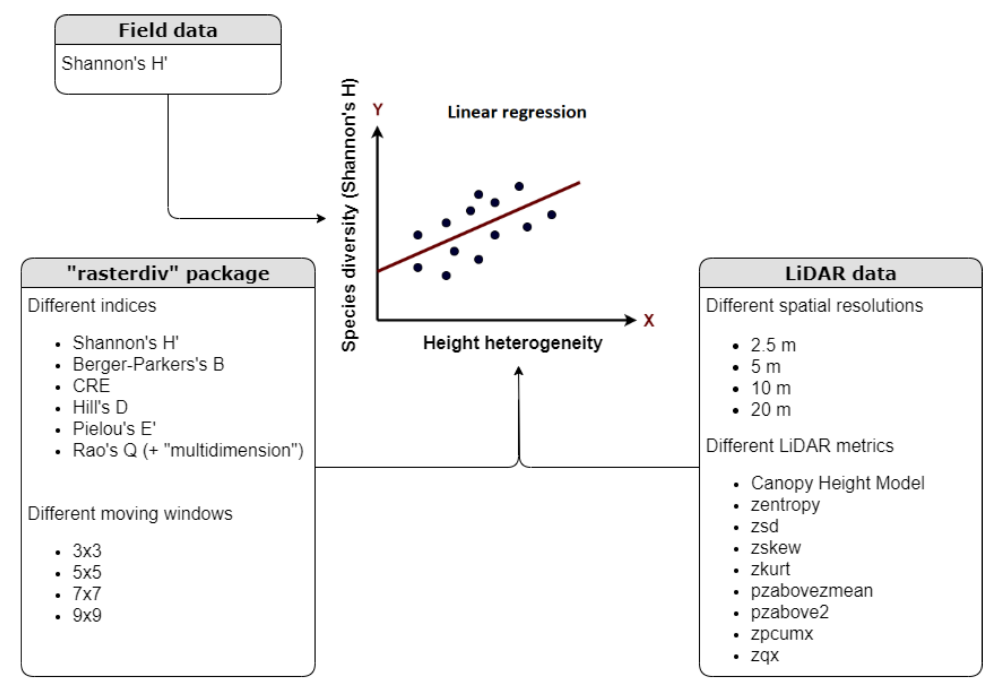
  • test different LiDAR metrics for the assessment of the HH;
  • understand which R rasterdiv index is the most accurate in characterizing the HH;
  • test the effects of different MW size for each index.

2. Materials and Methods

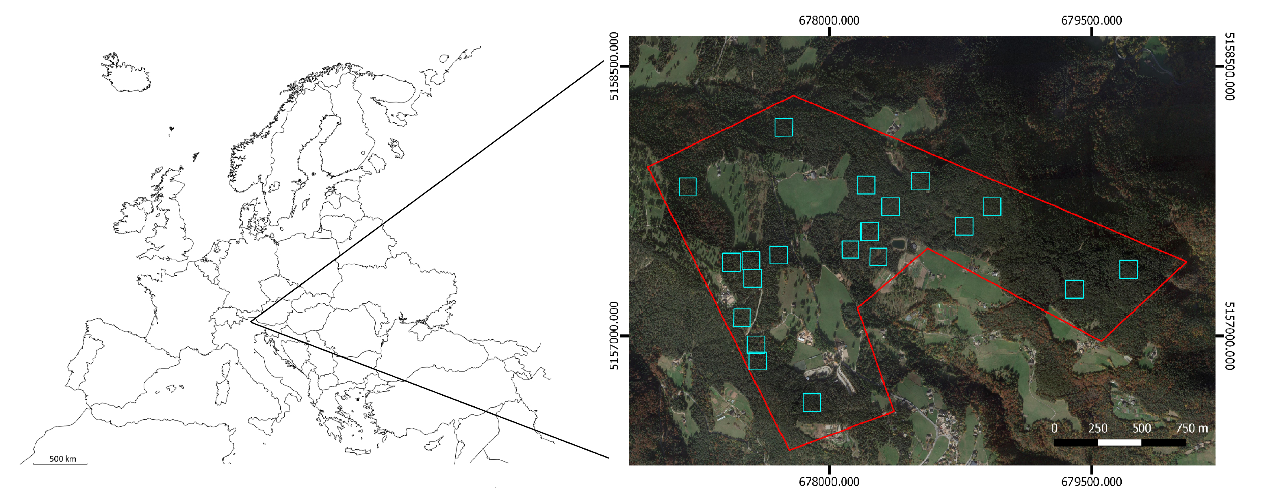
2.1. Study Area and Field Data

In this study, the HVH has been tested in the alpine coniferous forest located in the Province of Bolzano/Bozen (Italy) in the municipality of San Genesio/Jenesien (N46 55 E11 32 ). The size of the study area is approximately of 270 ha. Twenty plots having size of 1 ha (100 m × 100 m) were randomly chosen within a dense coniferous forest at 1100 m a.s.l (Figure 1). Following previous study designs [14,44], the center and corners of all plots were geo-referenced with a GPS device (spatial accuracy of ± 3 m; Garmin, Lenexa, KS, USA). From June to August 2017, within each plot, all the trees with a diameter at breast high (DBH) of at least 5 cm were measured with a tree caliper and classified into species. Ninety five percent of the measured trees were coniferous species, dominated by Pinus sylvestris, followed by Larix decidua and Picea abies. The remaining five percent were deciduous such as Betula alba, Corylus avellana, Salix caprea and Sorbus aucuparia.
In each plot, the Shannon’s H index (Equation (1)) was calculated in order to assess the tree species diversity [45].
H = i = 1 R p i ln ( p i ) ,
where:
  • H = Shannon’s H index.
  • R = number of species.
  • p i = proportion of species i relative to the total number of species.
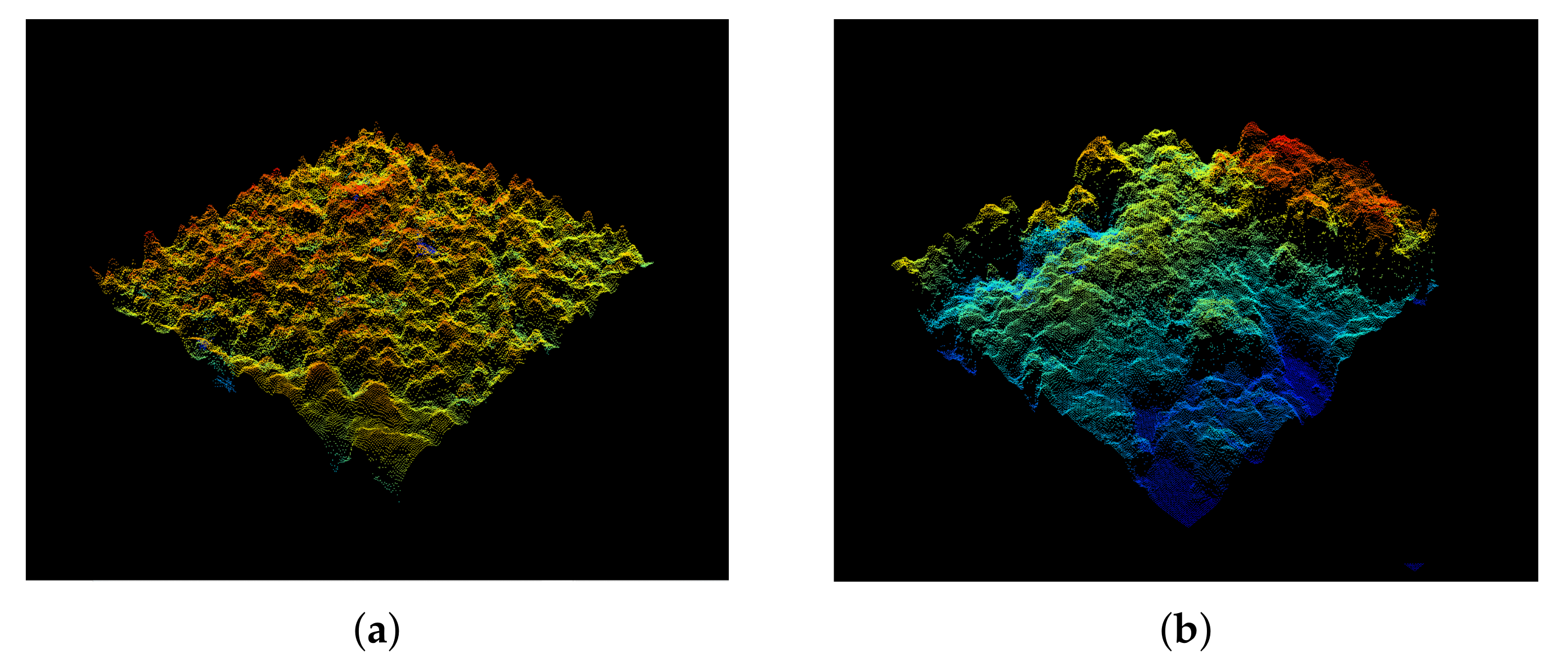
The Shannon’s H index has its foundations in information theory and it is widely used in ecological [46,47,48] and (more recently) in remote sensing applications [14].

2.2. LiDAR Data

The LiDAR data used in this study derives from an airborne laser scanning (ALS) campaign carried out in 2004–2006, acquired using ‘Optech ALTM 3033’ and ‘TopoSys Falcon II’ scanner systems. Recording accuracy and specifications of the two scanner systems used are shown in Table 1. Basic information on the ALS data acquisition was recorded during the flight with an integrated global positioning system (GPS) and an inertial measurement unit (IMU) [49].
The LiDAR point cloud, having a mean density of 2.9 point/m 2 , has been used to derive different LiDAR metrics. Firstly the ground points were classified with a progressive morphological filter [50]. The obtained point cloud was used to create a digital terrain model (DTM) through a triangular irregular network (TIN) combined with a Delaunay triangulation. The DTM was then used to normalize the point cloud. Finally, thanks to the R package lidR, the normalized point cloud was rasterized in order to obtain the canopy height models (CHM—as a difference between DSM and DTM) and the following LiDAR metrics at different spatial resolutions (2.5 m, 5 m, 10 m and 20 m):
  • zentropy: entropy of height distribution;
  • zmax: maximum height (in meters);
  • zsd: standard deviation of height distribution;
  • zskew: skewness of height distribution;
  • zkurt: kurtosis of height distribution;
  • pzabovezmean: percentage of returns above zmean;
  • pzabove2: percentage of returns above 2 m;
  • zpcumx: cumulative percentage of return in the xth layer according to Woods et al. [51];
  • zqx: percentile (quantile) of height distribution.
Although the field measurements were acquired in 2017, the temporal discrepancy between the ALS and the field campaigns did not affect our results, since limited forest management have occurred in the meantime in the forest area [14].

2.3. Height Heterogeneity Assessment and Statistical Analysis

Figure 2 summarizes the used methodology in order to test the HVH in the considered forest site of San Genesio/Jenesien. For each plot, all the R rasterdiv heterogeneity indices listed in Table 2 have been used to calculate the HH using all the available LiDAR metrics at four spatial resolutions (2.5 m, 5 m, 10 m, 20 m) using 4 different MWs: 3 × 3, 5 × 5, 7 × 7 and 9 × 9 (Figure A2). The Rao’s Q index has been also used through the multidimensional method (see Rocchini et al. [52] for further information) testing different metrics together. Table 3 reports the composition of the different lists used for this purpose. For each plot, a linear regression has been set between the in situ field data tree species diversity Shannon’s H index and the HHs calculated as the mean of each resulting matrix (derived from each index, calculated with the different LiDAR metrics and MWs).

3. Results

3.1. In-Situ Field Data Tree Species Diversity

Table 4 summarizes the Shannon’s H (used as in situ field data species diversity index) information related to the study area, while the Shannon’s H information for each plot is summarized in Table A1 (Appendix D).

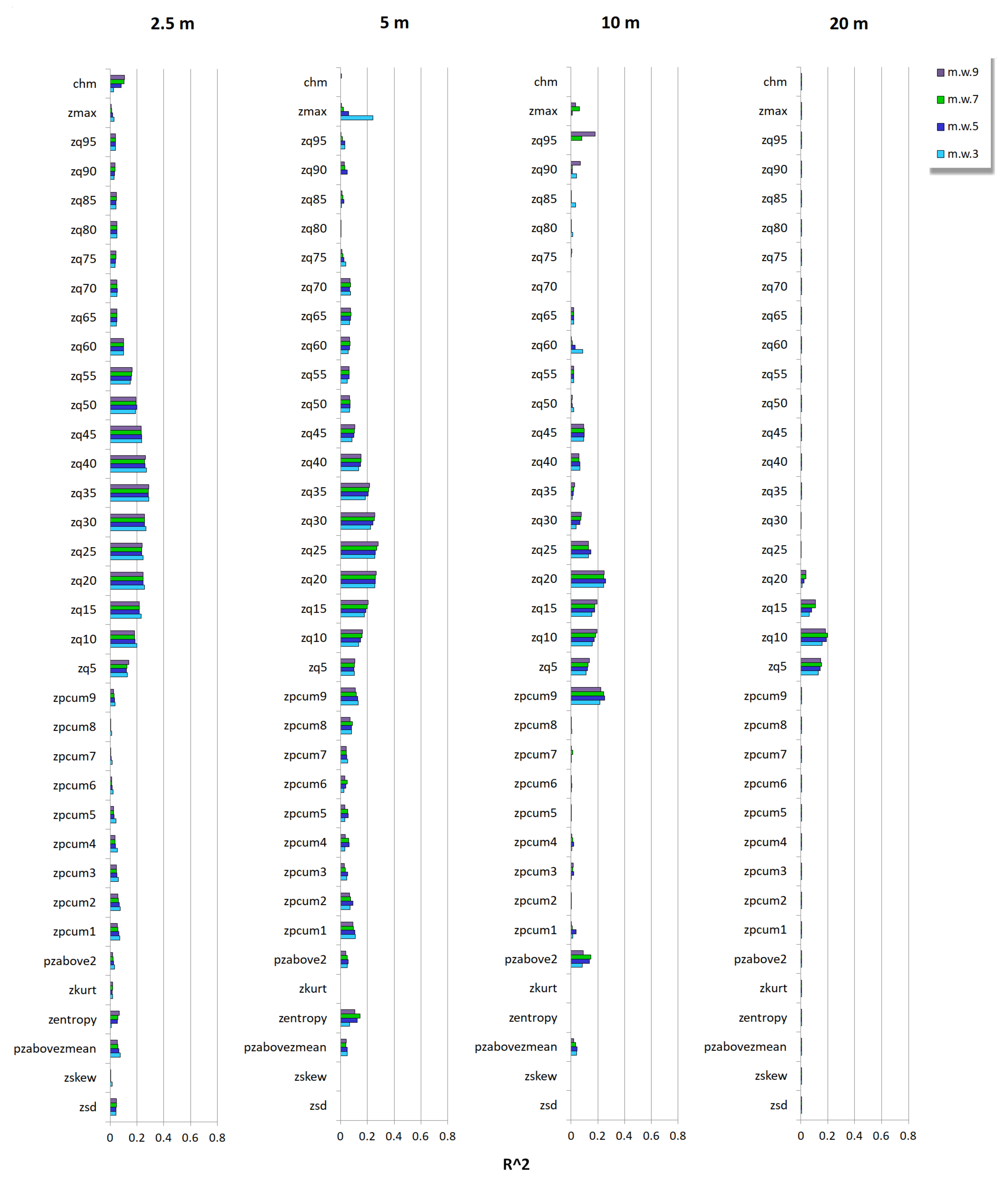
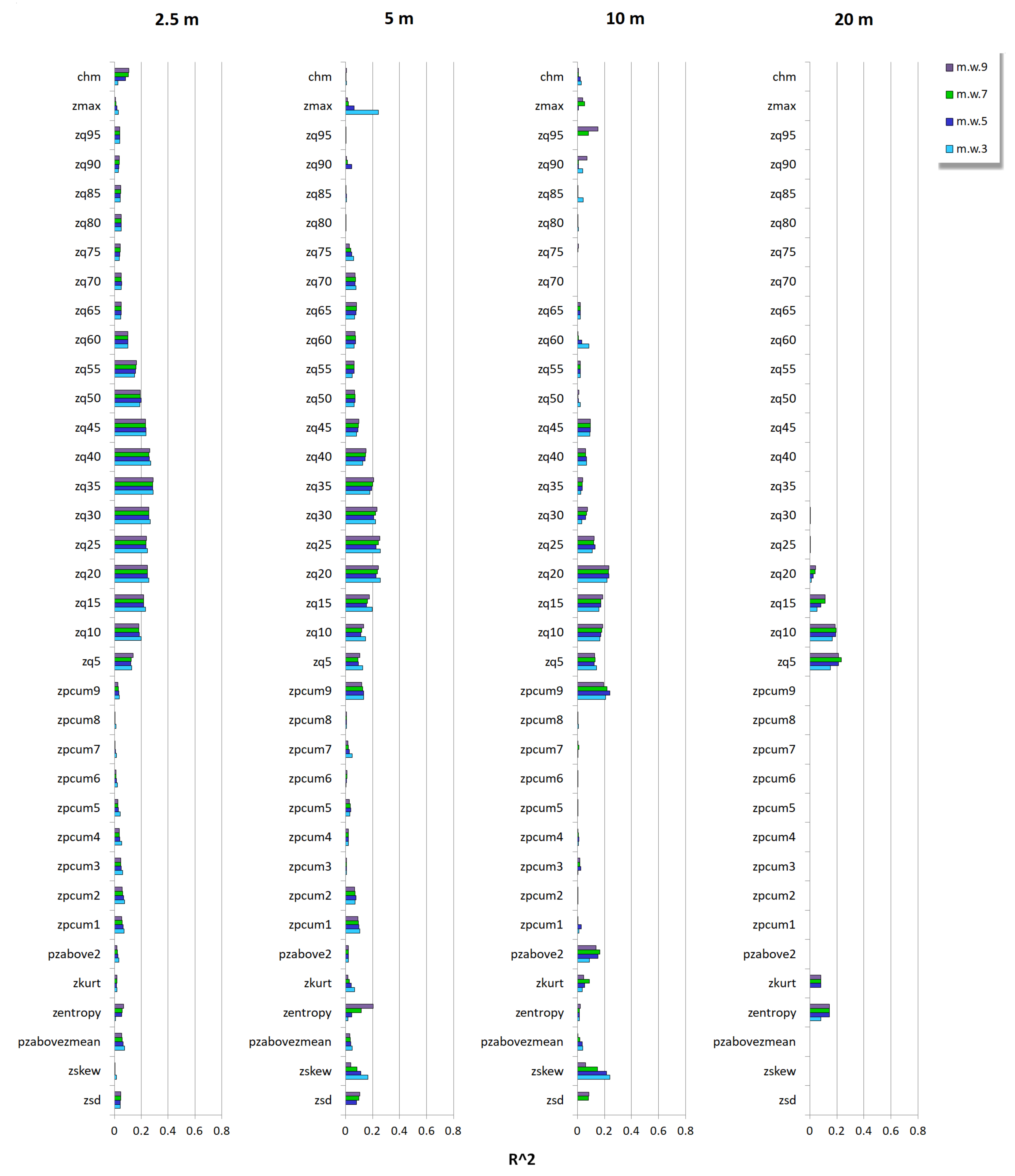
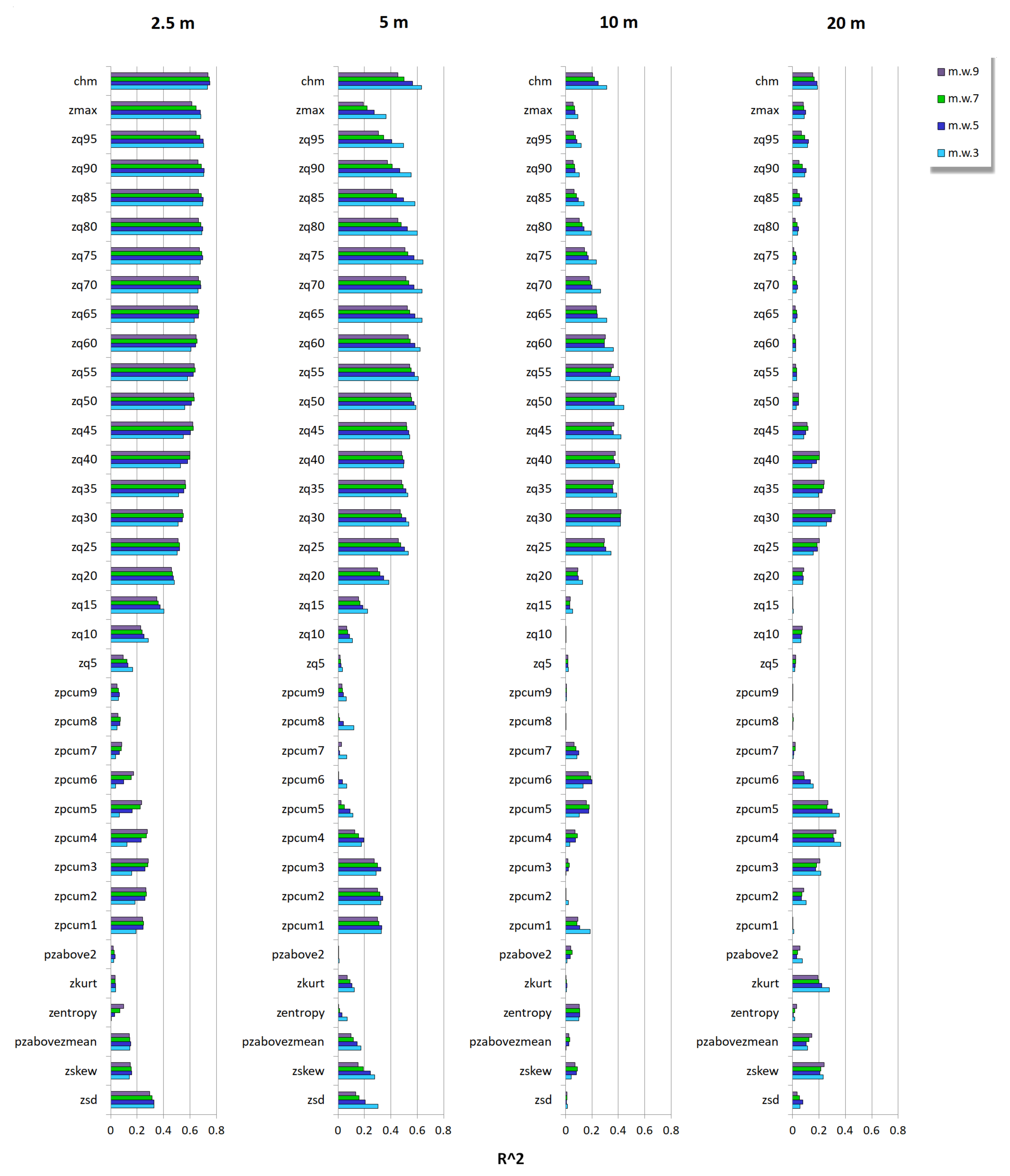
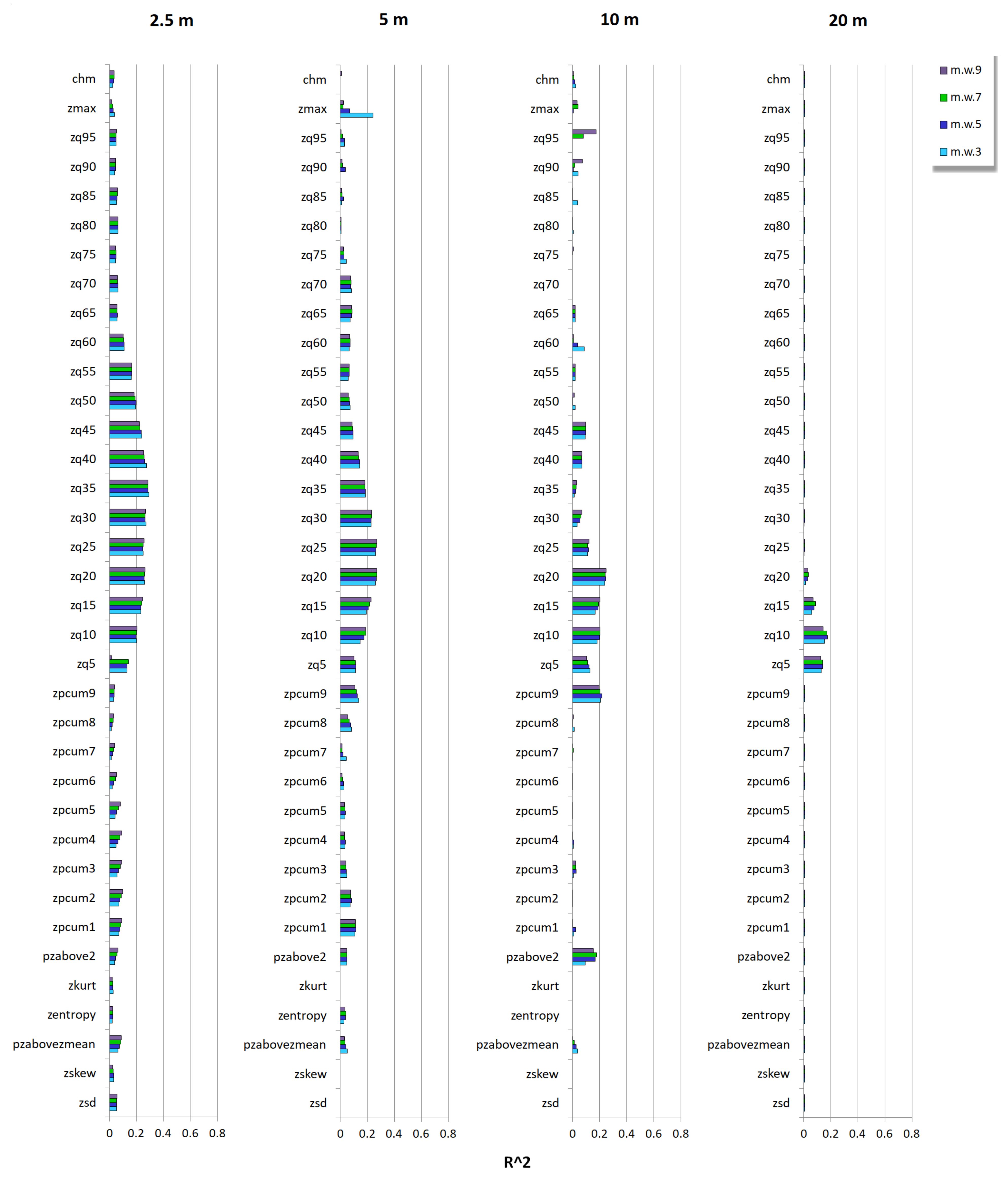
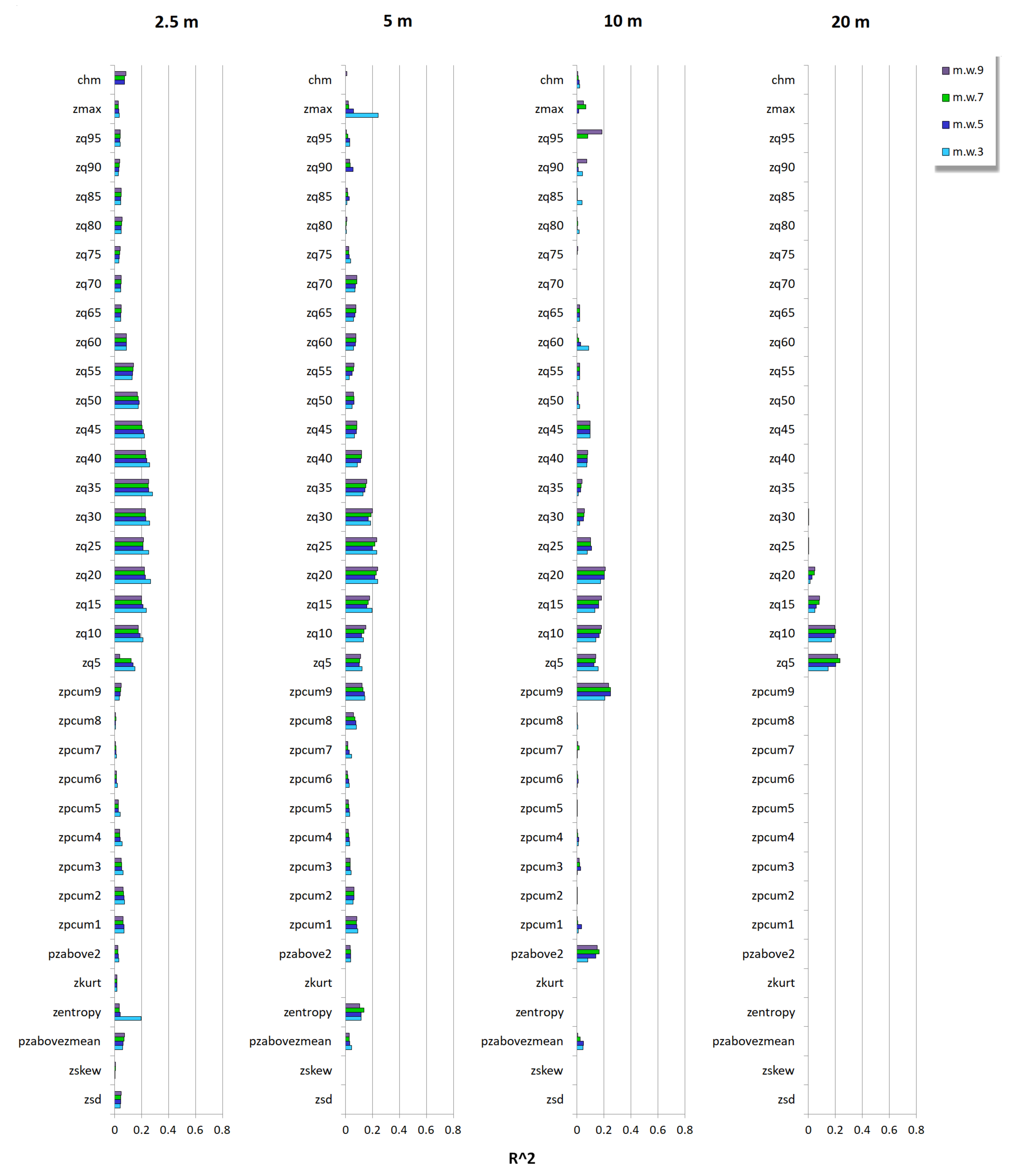
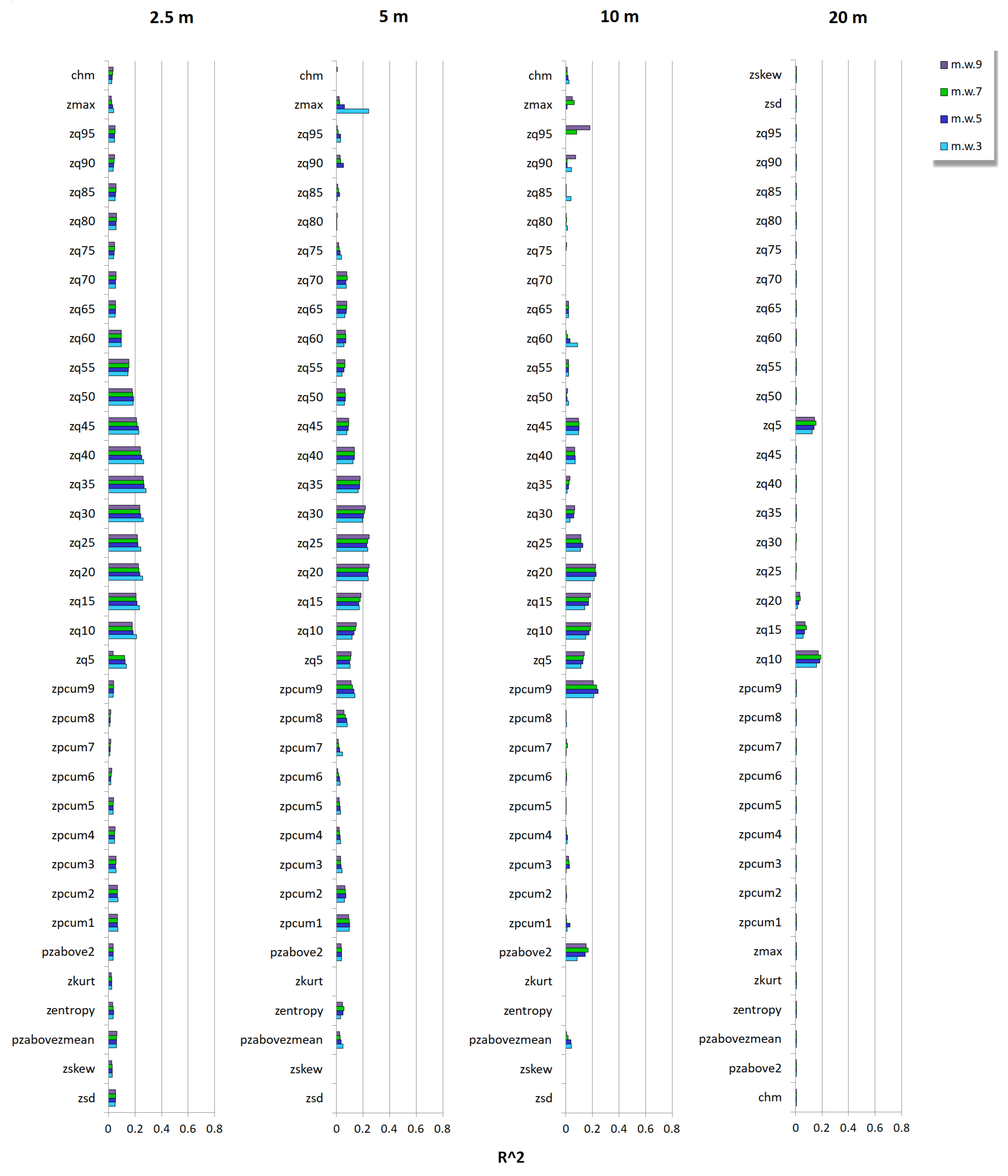
3.2. Relationship between Tree Species Diversity and LiDAR Height Heterogeneity

According to our results, the HVH tested on the coniferous forest of San Genesio/Jenesien can be considered a useful tool for assessing tree species diversity. The study showed that the results are influenced by both the LiDAR metrics and the heterogeneity indices, but not by the MW size. In particular, Figure 3 shows the histograms representing the R 2 values derived from the relationship between the Shannon’s field index and the HH, calculated for the Rao’s Q index using all the LiDAR metrics and MWs at different spatial resolutions (2.5 m, 5 m, 10 m and 20 m). In the Appendix C, we reported the histograms related to the other indices since they showed lower level of correlation. Best results have been obtained using Rao’s Q index at spatial resolution of 2.5 m ( R 2 ranging from 0.734 to 0.75—see Figure 3). Within this result, the LiDAR metrics that best related with the field’s tree species diversity (Shannon’s H) at spatial resolution of 2.5 m are the CHM and those related to the upper quantile point cloud distribution distribution (CHM, zq95, zq90, zq85, zq80). Similar results, with lower level of correlation are showed for the spatial resolution of 5 m. For a spatial resolution of 10 m, the correlations between HH and field data are lower, in this case the metrics that better correlate with the in situ field data diversity are the ones referred to the middle quantile distribution (zq50, zq45, zq30, zq55). Even lower are the levels of correlation for the spatial resolution of 20 m.
Particularly interesting are the Rao’s Q “multidimension” outcomes (Table 5). The lists 6 composed of “chm and zq95” at a spatial resolution of 2.5 m showed the highest correlation reaching R 2 values around 0.7 (the highest R 2 = 0.712 for a MW of 3 × 3).

4. Discussion

Different methods and approaches have been developed in recent years to assess various aspects of biodiversity through remote sensing data. The Height Variation Hypothesis (HVH) has proved to be one of them [28], stating that the higher the variation in tree height calculated from LiDAR data, the more complex the overall structure of the forest, and the higher the tree species diversity. Various studies showed that structurally complex forests increase biodiversity by enhancing environmental heterogeneity such as the variability of micro-habitats and the range of micro-climates [38,56], influencing not only the diversity of trees, but also of different other organisms including birds, small mammals and understory plants [38]. Height tree complexity is furthermore related to ecosystem productivity, by supporting complementary resource utilization among plant species [38]. The HVH takes advantages of the benefits of the LiDAR technology, which, with its high resolution, precision and increasing data availability, represents the perfect tool in forest applications for the 3D forest representation and its related vertical structure. In this study, the HVH has been tested using different LiDAR metrics, various heterogeneity indices and the MW approach in order to assess the relationship between the tree species diversity and the HH in an alpine coniferous forest located in the eastern Italian Alps. For the first time, all the R rasterdiv heterogeneity indices have been tested and compared in order to assess the environmental heterogeneity of various forest areas through the use of LiDAR data. The general outcomes showed that the HVH can be considered an effective tool for the assessment of tree species diversity in forest ecosystems, where the selection of specific LiDAR metrics and heterogeneity indices play a crucial role in the final results.
The results of this study showed that, within all the used combinations of LiDAR metrics and MWs, the Rao’s Q heterogeneity index, used to assess the HH, performed better than the other indices. Once the index is used on one single layer, as carried out in the “single dimension” analysis of this paper, half of the squared Euclidean distance (1/2 d i j 2 where d i j is the Euclidean distance) is used and the Rao’s Q reduces to variance, which is basically a good approximation of heterogeneity when making use of continuous variables [57]. In the “multidimensional mode”, each distance is multiplied by the inverse of the squared number of pixels in the considered MW, and the Rao’s Q is finally derived by applying their summation. Furthermore the Rao’s Q, compared to the other considered indices, has the characteristic of considering both the distance (using their values) and abundance of the pixels within a considered dataset [58]. This result is in line with several other studies where the Rao’s Q index has been used to assess biodiversity in different ecosystems [14,59,60]. We refer to [61,62,63] for additional information on the mathematical properties of Rao’s Q.
The outcomes showed that certain LiDAR metrics, within the concept of the HVH, are more suitable for assessing HH. Generally, using the Rao’s Q index as heterogeneity index, the LiDAR metrics related to the upper quantile point cloud distribution (CHM, zp95, zp90, zp85) with at a fine spatial resolutions (2.5 m and 5 m) showed the most accurate results. The outcomes related to the multidimensional Rao’s Q index are in line with the general results referred to the single metrics. The highest levels of correlation are found using the “list 6” that includes both the CHM and the zq95. These results highlight that the HVH is mainly influenced by those metrics (CHM and upper quantile point cloud distribution) that characterize the forest canopy and the related forest structure. These outcomes are in line with the previous study of Torresani et al. [28], where the HVH was tested also in the study area of San Genesio/Jenesien, using only the CHM LiDAR metric.
As previously stressed, in the study of Torresani et al. [28], the HVH has been tested in the area of San Genesio/Jenesien correlating the HH with the Rao’s Q index only using the CHM (without MW) reaching a R 2 value of 0.63 (using a CHM with a resolution of 2.5 m). In this study, in the same study area, using a CHM of the same spatial resolution, applying the MW approach, the R 2 ranged from 0.734 to 0.75, showing that this technique could add more precision to the estimation of the HH.
The spatial resolution of the LiDAR data played a crucial role in this study. As shown in the results related to the Rao’s Q index, the different LiDAR metrics have been tested at different resolutions, in order to understand how the HH changes using datasets with different pixel sizes. In our study, the coarser area resolutions generated the weakest results. These results are again in line with the previous study of Torresani et al. [28], where the relationship between HH and species diversity was stronger for finer resolutions (2.5 m). The authors stated that in dense forest areas such as the one of San Genesio/Jenesien, this resolution could be considered the most appropriate for the detection of single trees. The essential concept behind the HVH is that the HH should reflect the trees’ heterogeneity; therefore, a too high or too coarse LiDAR metric resolution risks being inappropriate for our purpose. As stated in various other studies [28,64], the relation of higher spatial resolution—higher accuracy is not always so clear and linear. Sometimes, within an image, too high resolutions bring too much noise and variability when compared to the size of the target objects of the study, thus reducing accuracy. One of the challenges, therefore, is to ensure that the scales of the images match those of the species richness data, and that both are properly scaled [65].
This study was possible thanks to the new R rasterdiv package that allows us to conduct multi-scale studies, giving the possibility to choose different indices and MW sizes, combining them at different spatial resolutions. These features allow the researchers to make the scale factor explicit when performing spatial analysis and to avoid scale-related confusion effects in the calculation of diversity measures. The different features of the package allow to reduce the problems of hidden patterns within the relation between field and landscape based diversity caused by scale mismatch [42,66]. In this study, for the first time, the R rasterdiv package was tested with remote sensing information having field validation data, showing its skills as a possible benchmark R package for the assessment of remote sensing biodiversity.
An additional concern that may arise could be related to the small extent of the study area, an alpine coniferous forest dominated mainly by pines, larches and spruces. Other related studies tested similar concepts (like the Spectral Variation Hypothesis—SVH) in relatively small areas, considering a limited number of plots. Gould et al. [67] tested the SVH in the Hood river region of the central Canadian arctic using 17 plots of 0.5 km 2 size. Rocchini et al. [68] used 22 plots to test the spectral variation of multispectral images for the estimation of the species diversity in a wetland area in Central Italy. This study represents one of the first steps in order to explain the relation between the tree species diversity and HH since, to date, only one other study [28] has focused on investigating the HVH. This point represents a typical bias of any empirical study, and due to the strength of the general relation between HH and species diversity, the results of this research can probably be applicable to wider areas. Concluding, it is worth underlining that, as stated by Torresani et al. [28], the concept of HVH might not always hold truth in all the considered ecosystems. Some forests might have a high structural diversity that does not correspond to a high tree species diversity. Typical examples of these environments are some natural forests in ‘climax’ stage, like the alpine larch forests found at the limit of vegetation. These forests are indeed characterized by a high structural diversity and low tree species diversity, due to the low competition given by the particular climatic conditions.

5. Conclusions

In this paper, the concept of HVH proposed by Torresani et al. [28] was covered in depth, testing the above mention hypothesis in an alpine coniferous forest in the eastern Italian Alps, using different LiDAR metrics, heterogeneity indices (thanks to the R rasterdiv package) and MWs approaches. The results showed that in general, the concept of HVH holds truth with the Rao’s Q heterogeneity index using LiDAR metrics related to the canopy of the forest (CHM and the ones associated to upper quantile point cloud distribution distribution) applied to fine spatial resolutions (of 2.5 m and 5 m). However, we are aware that the suggested hypothesis should be tested in other forest ecosystems, using different indices and data-sets, before considering the approach a generalizable method. Further analysis could be conducted by developing a methodology that combines information from optical sensors, with the aim of obtaining multiple types of information. Additional analysis could consider the species diversity of forest shrubs, grasses or animals in order to have a more complete biodiversity picture of the forest. We suggest the HVH could be used as a ‘first filter’ in the identification of tree species diversity hot-spots by forest manager or ecologists, or eventually to guide field sampling.

Author Contributions

Conceptualization, D.R.; validation, M.T.; formal analysis, D.T.; investigation, G.T.; data curation, E.T.; writing—original draft, D.T.; writing—review and editing, M.T.; supervision, D.R.; project administration, D.R. All authors have read and agreed to the published version of the manuscript.

Funding

M.T. and D.R. were partially supported by the H2020 Project SHOWCASE (Grant agreement nr. 862480). D.R. was partially supported by the H2020 COST Action CA17134 ‘Optical synergies for spatiotemporal sensing of scalable ecophysiological traits (SENESCO)’.

Institutional Review Board Statement

Not applicable.

Informed Consent Statement

Not applicable.

Data Availability Statement

Data are available from the corresponding author upon reasonable request.

Conflicts of Interest

The authors declare no conflict of interest.

Abbreviations

The following abbreviations are used in this manuscript:
HHHeight Heterogeneity
HVHHeight Variation Hypothesis
SVHSpectral Variation Hypothesis
MWMoving Window
CHMCanopy Height Model
DTMDigital Terrain Model
DSMDigital Surface Model
ALSAirborne Laser Scanning
TLSTerrestrial Laser Scanning
TINTriangular Irregular Network
DBHDiameter at Breast High
zentropyEntropy of height distribution
zmaxMaximum height (in meters)
zsdStandard deviation of height distribution
zskewSkewness of height distribution
zkurtKurtosis of height distribution
pzabovezmeanPercentage of returns above zmean
pzabove2Percentage of returns above 2 m
zpcumxCumulative percentage of return in the xth layer according to Woods et al. [51]
zqxPercentile (quantile) of height distribution

Appendix A. Visual Representation Height Variation Hypothesis

Figure A1. Visual representation of the “Height Variation Hypothesis”: the subfigure (a) shows the LiDAR point cloud over a forest plot (1 ha) having a low height heterogeneity and a low species diversity. On the other side, plot (b) shows a higher height heterogeneity and a related higher species diversity.
Remotesensing 13 03569 g0a1

Appendix B. Moving Windows and Spatial Resolution

Figure A2. Representation of moving windows (3 × 3, 5 × 5, 7 × 7, 9 × 9) applied to 10 m of spatial resolution.
Remotesensing 13 03569 g0a2

Appendix C. San Genesio/Jenesien Histograms

Appendix C.1. Berger-Parker

Figure A3. Histograms concerning the R 2 values relative to the linear regression between Shannon’s H field index and the mean of the Berger–Parker’s matrices of each LiDAR metric and for each MW (San Genesio/Jenesien study area).
Remotesensing 13 03569 g0a3

Appendix C.2. CRE

Figure A4. Histograms concerning the R 2 values relative to the linear regression between Shannon’s H field index and the mean of the CRE matrices of each LiDAR metric and for each MW (San Genesio/Jenesien study area).
Remotesensing 13 03569 g0a4

Appendix C.3. Hill

Figure A5. Histograms concerning the R 2 values relative to the linear regression between Shannon’s H field index and the mean of the Hill’s matrices of each LiDAR metric and for each MW (San Genesio/Jenesien study area).
Remotesensing 13 03569 g0a5

Appendix C.4. Pielou

Figure A6. Histograms concerning the R 2 values relative to the linear regression between Shannon’s H field index and the mean of the Pielou’s matrices of each LiDAR metric and for each MW (San Genesio/Jenesien study area).
Remotesensing 13 03569 g0a6

Appendix C.5. Shannon’s H

Figure A7. Histograms concerning the R 2 values relative to the linear regression between Shannon’s H field index and the mean of the Shannon’s H matrices of each LiDAR metric and for each MW (San Genesio/Jenesien study area).
Remotesensing 13 03569 g0a7

Appendix D. Field Data Shannon’s H

Table A1. Shannon’s H and species richness for each of the 20 plots.
Plot NumberShannon’s HSpecies Richness
10.115
20.987
31.3611
40.949
51.054
60.84
70.554
80.966
90.886
100.447
110.659
120.828
130.677
140.326
150.127
160.424
170.445
180.277
190.946
200.74

References

  1. Mace, G.M.; Norris, K.; Fitter, A.H. Biodiversity and ecosystem services: A multilayered relationship. Trends Ecol. Evol. 2012, 27, 19–26. [Google Scholar] [CrossRef] [PubMed]
  2. Lindenmayer, D.; Franklin, J.; Fischer, J. General management principles and a checklist of strategies to guide forest biodiversity conservation. Biol. Conserv. 2006, 131, 433–445. [Google Scholar] [CrossRef]
  3. Gamfeldt, L.; Snäll, T.; Bagchi, R.; Jonsson, M.; Gustafsson, L.; Kjellander, P.; Ruiz-Jaen, M.C.; Fröbeg, M.; Stendahl, J.; Philipson, C.D.; et al. Higher levels of multiple ecosystem services are found in forests with more tree species. Nat. Commun. 2013, 4, 1340. [Google Scholar] [CrossRef] [PubMed]
  4. Mori, A.S.; Lertzman, K.P.; Gustafsson, L. Biodiversity and ecosystem services in forest ecosystems: A research agenda for applied forest ecology. J. Appl. Ecol. 2017, 54, 12–27. [Google Scholar] [CrossRef]
  5. Brockerhoff, E.G.; Barbaro, L.; Castagneyrol, B.; Forrester, D.I.; Gardiner, B.; González-Olabarria, J.R.; Lyver, P.O.; Meurisse, N.; Oxbrough, A.; Taki, H.; et al. Forest biodiversity, ecosystem functioning and the provision of ecosystem services. Biodivers. Conserv. 2017, 26, 3005–3035. [Google Scholar] [CrossRef] [Green Version]
  6. Ball, B.A.; Bradford, M.A.; Coleman, D.C.; Hunter, M.D. Linkages between below and aboveground communities: Decomposer responses to simulated tree species loss are largely additive. Soil Biol. Biochem. 2009, 41, 1155–1163. [Google Scholar] [CrossRef]
  7. Kobayashi, Y.; Mori, A.S. The potential role of tree diversity in reducing shallow landslide risk. Environ. Manag. 2017, 59, 807–815. [Google Scholar] [CrossRef]
  8. Castagneyrol, B.; Jactel, H. Unraveling plant–animal diversity relationships: A meta-regression analysis. Ecology 2012, 93, 2115–2124. [Google Scholar] [CrossRef]
  9. Hanski, I. Habitat loss, the dynamics of biodiversity, and a perspective on conservation. Ambio 2011, 40, 248–255. [Google Scholar] [CrossRef] [Green Version]
  10. Cayuela, L.; Golicher, D.J.; Benayas, J.M.R.; González-Espinosa, M.; Ramírez, N. Fragmentation, disturbance and tree diversity conservation in tropical montane forests. J. Appl. Ecol. 2006, 43, 1172–1181. [Google Scholar] [CrossRef]
  11. Chaudhary, A.; Burivalova, Z.; Koh, L.P.; Hellweg, S. Impact of forest management on species richness: Global meta-analysis and economic trade-offs. Sci. Rep. 2016, 6, 23954. [Google Scholar] [CrossRef] [PubMed] [Green Version]
  12. Bellard, C.; Bertelsmeier, C.; Leadley, P.; Thuiller, W.; Courchamp, F. Impacts of climate change on the future of biodiversity. Ecol. Lett. 2012, 15, 365–377. [Google Scholar] [CrossRef] [PubMed] [Green Version]
  13. McNeely, J.A. The sinking ark: Pollution and the worldwide loss of biodiversity. Biodivers. Conserv. 1992, 1, 2–18. [Google Scholar] [CrossRef]
  14. Torresani, M.; Rocchini, D.; Sonnenschein, R.; Zebisch, M.; Marcantonio, M.; Ricotta, C.; Tonon, G. Estimating tree species diversity from space in an alpine conifer forest: The Rao’s Q diversity index meets the spectral variation hypothesis. Ecol. Inform. 2019, 52, 26–34. [Google Scholar] [CrossRef] [Green Version]
  15. Rocchini, D.; Luque, S.; Pettorelli, N.; Bastin, L.; Doktor, D.; Faedi, N.; Feilhauer, H.; Féret, J.B.; Foody, G.M.; Gavish, Y.; et al. Measuring β-diversity by remote sensing: A challeg, for biodiversity monitoring. Methods Ecol. Evol. 2018, 9, 1787–1798. [Google Scholar] [CrossRef] [Green Version]
  16. Lausch, A.; Bannehr, L.; Beckmann, M.; Boehm, C.; Feilhauer, H.; Hacker, J.; Heurich, M.; Jung, A.; Klenke, R.; Neumann, C.; et al. Linking Earth Observation and taxonomic, structural and functional biodiversity: Local to ecosystem perspectives. Ecol. Indic. 2016, 70, 317–339. [Google Scholar] [CrossRef]
  17. Rocchini, D.; Balkenhol, N.; Carter, G.A.; Foody, G.M.; Gillespie, T.W.; He, K.S.; Kark, S.; Levin, N.; Lucas, K.; Luoto, M.; et al. Remotely sensed spectral heterogeneity as a proxy of species diversity: Recent advances and open challenges. Ecol. Inform. 2010, 5, 318–329. [Google Scholar] [CrossRef]
  18. Rocchini, D.; Marcantonio, M.; Da Re, D.; Chirici, G.; Galluzzi, M.; Lenoir, J.; Ricotta, C.; Torresani, M.; Ziv, G. Time-lapsing biodiversity: An open source method for measuring diversity changes by remote sensing. Remote Sens. Environ. 2019, 231, 111192. [Google Scholar] [CrossRef] [Green Version]
  19. Rocchini, D.; Salvatori, N.; Beierkuhnlein, C.; Chiarucci, A.; de Boissieu, F.; Förster, M.; Garzon-Lopez, C.X.; Gillespie, T.W.; Hauffe, H.C.; He, K.S.; et al. From local spectral species to global spectral communities: A benchmark for ecosystem diversity estimate by remote sensing. Ecol. Inform. 2021, 61, 101195. [Google Scholar] [CrossRef]
  20. Dalponte, M.; Marzini, S.; Solano-Correa, Y.T.; Tonon, G.; Vescovo, L.; Gianelle, D. Mapping forest windthrows using high spatial resolution multispectral satellite images. Int. J. Appl. Earth Obs. Geoinf. 2020, 93, 102206. [Google Scholar] [CrossRef]
  21. Rocchini, D.; Hernández-Stefanoni, J.L.; He, K.S. Advancing species diversity estimate by remotely sensed proxies: A conceptual review. Ecol. Inform. 2015, 25, 22–28. [Google Scholar] [CrossRef]
  22. Rocchini, D.; Andreo, V.; Förster, M.; Garzon-Lopez, C.X.; Gutierrez, A.P.; Gillespie, T.W.; Hauffe, H.C.; He, K.S.; Kleinschmit, B.; Mairota, P.; et al. Potential of remote sensing to predict species invasions: A modelling perspective. Prog. Phys. Geogr. 2015, 39, 283–309. [Google Scholar] [CrossRef] [Green Version]
  23. Torresani, M.; Feilhauer, H.; Rocchini, D.; Féret, J.B.; Zebisch, M.; Tonon, G. Which optical traits enable an estimation of tree species diversity based on the Spectral Variation Hypothesis? Appl. Veg. Sci. 2021, 24, e12586. [Google Scholar] [CrossRef]
  24. Sakowska, K.; MacArthur, A.; Gianelle, D.; Dalponte, M.; Alberti, G.; Gioli, B.; Miglietta, F.; Pitacco, A.; Meggio, F.; Fava, F.; et al. Assessing across-scale optical diversity and productivity relationships in grasslands of the Italian Alps. Remote Sens. 2019, 11, 614. [Google Scholar] [CrossRef] [Green Version]
  25. Xie, Y.; Sha, Z.; Yu, M. Remote sensing imagery in vegetation mapping: A review. J. Plant Ecol. 2008, 1, 9–23. [Google Scholar] [CrossRef]
  26. Wulder, M.A.; Hall, R.J.; Coops, N.C.; Franklin, S.E. High spatial resolution remotely sensed data for ecosystem characterization. BioScience 2004, 54, 511–521. [Google Scholar] [CrossRef] [Green Version]
  27. Wüest, R.O.; Bergamini, A.; Bollmann, K.; Baltensweiler, A. LiDAR data as a proxy for light availability improve distribution modelling of woody species. For. Ecol. Manag. 2020, 456, 117644. [Google Scholar] [CrossRef]
  28. Torresani, M.; Rocchini, D.; Sonnenschein, R.; Zebisch, M.; Hauffe, H.C.; Heym, M.; Pretzsch, H.; Tonon, G. Height variation hypothesis: A new approach for estimating forest species diversity with CHM LiDAR data. Ecol. Indic. 2020, 117, 106520. [Google Scholar] [CrossRef]
  29. Moudrỳ, V.; Moudrá, L.; Barták, V.; Bejček, V.; Gdulová, K.; Hendrychová, M.; Moravec, D.; Musil, P.; Rocchini, D.; Št’astnỳ, K.; et al. The role of the vegetation structure, primary productivity and senescence derived from airborne LiDAR and hyperspectral data for birds diversity and rarity on a restored site. Landsc. Urban Plan. 2021, 210, 104064. [Google Scholar] [CrossRef]
  30. Maltamo, M.; Næsset, E.; Vauhkonen, J. Forestry applications of airborne laser scanning. Concepts Case Stud. Manag. Ecosyst. 2014, 27, 2014. [Google Scholar]
  31. Holopainen, M.; Kankare, V.; Vastaranta, M.; Liang, X.; Lin, Y.; Vaaja, M.; Yu, X.; Hyyppä, J.; Hyyppä, H.; Kaartinen, H.; et al. Tree mapping using airborne, terrestrial and mobile laser scanning–A case study in a heterogeneous urban forest. Urban For. Urban Green. 2013, 12, 546–553. [Google Scholar] [CrossRef]
  32. Guo, X.; Coops, N.C.; Tompalski, P.; Nielsen, S.E.; Bater, C.W.; Stadt, J.J. Regional mapping of vegetation structure for biodiversity monitoring using airborne lidar data. Ecol. Inform. 2017, 38, 50–61. [Google Scholar] [CrossRef]
  33. Hakkenbeg, C.R.; Song, C.; Peet, R.K.; White, P.S. Forest structure as a predictor of tree species diversity in the North Carolina Piedmont. J. Veg. Sci. 2016, 27, 1151–1163. [Google Scholar] [CrossRef]
  34. Bohn, F.J.; Huth, A. The importance of forest structure to biodiversity–productivity relationships. R. Soc. Open Sci. 2017, 4, 160521. [Google Scholar] [CrossRef] [PubMed] [Green Version]
  35. Echeverría, C.; Newton, A.C.; Lara, A.; Benayas, J.M.R.; Coomes, D.A. Impacts of forest fragmentation on species composition and forest structure in the temperate landscape of southern Chile. Glob. Ecol. Biogeogr. 2007, 16, 426–439. [Google Scholar] [CrossRef] [Green Version]
  36. Walter, J.A.; Stovall, A.E.; Atkins, J.W. Vegetation structural complexity and biodiversity in the Great Smoky Mountains. Ecosphere 2021, 12, e03390. [Google Scholar] [CrossRef]
  37. Frazer, G.W.; Wulder, M.A.; Niemann, K.O. Simulation and quantification of the fine-scale spatial pattern and heterogeneity of forest canopy structure: A lacunarity-based method designed for analysis of continuous canopy heights. For. Ecol. Manag. 2005, 214, 65–90. [Google Scholar] [CrossRef]
  38. Ishii, H.T.; Tanabe, S.i.; Hiura, T. Exploring the relationships among canopy structure, stand productivity, and biodiversity of temperate forest ecosystems. For. Sci. 2004, 50, 342–355. [Google Scholar]
  39. Alberti, G.; Boscutti, F.; Pirotti, F.; Bertacco, C.; De Simon, G.; Sigura, M.; Cazorzi, F.; Bonfanti, P. A LiDAR-based approach for a multi-purpose characterization of Alpine forests: An Italian case study. Iforest-Biogeosci. For. 2013, 6, 156. [Google Scholar] [CrossRef]
  40. Huang, Q.; Swatantran, A.; Dubayah, R.; Goetz, S.J. The influence of vegetation height heterogeneity on forest and woodland bird species richness across the United States. PLoS ONE 2014, 9, e103236. [Google Scholar]
  41. Palmer, M.W.; Earls, P.G.; Hoagland, B.W.; White, P.S.; Wohlgemuth, T. Quantitative tools for perfecting species lists. Environ. Off. J. Int. Environ. Soc. 2002, 13, 121–137. [Google Scholar] [CrossRef]
  42. Thouverai, E.; Marcantonio, M.; Bacaro, G.; Da Re, D.; Iannacito, M.; Ricotta, C.; Tattoni, C.; Vicario, S.; Rocchini, D. Measuring diversity from space: A global view of the free and open source rasterdiv R package under a coding perspective. Community Ecol. 2021, 22, 1–11. [Google Scholar] [CrossRef]
  43. Rocchini, D.; Thouverai, E.; Marcantonio, M.; Iannacito, M.; Da Re, D.; Torresani, M.; Bacaro, G.; Bazzichetto, M.; Bernardi, A.; Foody, G.M.; et al. rasterdiv—An Information Theory tailored R package for measuring ecosystem heterogeneity from space: To the origin and back. Methods Ecol. Evol. 2021, 12, 1093–1102. [Google Scholar] [CrossRef] [PubMed]
  44. Cao, M.; Zhang, J. Tree species diversity of tropical forest vegetation in Xishuangbanna, SW China. Biodivers. Conserv. 1997, 6, 995–1006. [Google Scholar] [CrossRef]
  45. Shannon, C.E. A mathematical theory of communication. Bell Syst. Tech. J. 1948, 27, 379–423. [Google Scholar] [CrossRef] [Green Version]
  46. Spellerbeg, I.F.; Fedor, P.J. A tribute to Claude Shannon (1916–2001) and a plea for more rigorous use of species richness, species diversity and the ‘Shannon–Wiener’Index. Glob. Ecol. Biogeogr. 2003, 12, 177–179. [Google Scholar] [CrossRef] [Green Version]
  47. Fierer, N.; Jackson, R.B. The diversity and biogeography of soil bacterial communities. Proc. Natl. Acad. Sci. USA 2006, 103, 626–631. [Google Scholar] [CrossRef] [Green Version]
  48. Gaudeul, M.; Taberlet, P.; Till-Bottraud, I. Genetic diversity in an endangered alpine plant, Eryngium alpinum L. (Apiaceae), inferred from amplified fragment length polymorphism markers. Mol. Ecol. 2000, 9, 1625–1637. [Google Scholar] [CrossRef] [Green Version]
  49. Knoll, C.; Kerschner, H. A glacier inventory for South Tyrol, Italy, based on airborne laser-scanner data. Ann. Glaciol. 2009, 50, 46–52. [Google Scholar] [CrossRef] [Green Version]
  50. Zhang, K.; Chen, S.C.; Whitman, D.; Shyu, M.L.; Yan, J.; Zhang, C. A progressive morphological filter for removing nonground measurements from airborne LIDAR data. IEEE Trans. Geosci. Remote Sens. 2003, 41, 872–882. [Google Scholar] [CrossRef] [Green Version]
  51. Woods, M.; Lim, K.; Treitz, P. Predicting forest stand variables from LIDAR data in the Great Lakes St. Lawrence Forest of Ontario. For. Chron. 2008, 84, 827–839. [Google Scholar] [CrossRef] [Green Version]
  52. Rocchini, D.; Marcantonio, M.; Ricotta, C. Measuring Rao’s Q diversity index from remote sensing: An open source solution. Ecol. Indic. 2017, 72, 234–238. [Google Scholar] [CrossRef]
  53. Caruso, T.; Pigino, G.; Bernini, F.; Bargagli, R.; Migliorini, M. The Berger–Parker index as an effective tool for monitoring the biodiversity of disturbed soils: A case study on Mediterranean oribatid (Acari: Oribatida) assemblages. In Biodiversity and Conservation in Europe; Springer: Berlin/Heidelbeg, Germany, 2006; pp. 35–43. [Google Scholar]
  54. Rao, M.; Chen, Y.; Vemuri, B.C.; Wang, F. Cumulative residual entropy: A new measure of information. IEEE Trans. Inf. Theory 2004, 50, 1220–1228. [Google Scholar] [CrossRef]
  55. Chao, A.; Chiu, C.H.; Jost, L. Phylogenetic diversity measures based on Hill numbers. Philos. Trans. R. Soc. B Biol. Sci. 2010, 365, 3599–3609. [Google Scholar] [CrossRef]
  56. Schall, P.; Schulze, E.D.; Fischer, M.; Ayasse, M.; Ammer, C. Relations between forest management, stand structure and productivity across different types of Central European forests. Basic Appl. Ecol. 2018, 32, 39–52. [Google Scholar] [CrossRef]
  57. Laliberté, E.; Schweiger, A.K.; Legendre, P. Partitioning plant spectral diversity into alpha and beta components. Ecol. Lett. 2020, 23, 370–380. [Google Scholar] [CrossRef] [PubMed] [Green Version]
  58. Rao, C.R. Diversity and dissimilarity coefficients: A unified approach. Theor. Popul. Biol. 1982, 21, 24–43. [Google Scholar] [CrossRef]
  59. Khare, S.; Latifi, H.; Rossi, S. Forest beta-diversity analysis by remote sensing: How scale and sensors affect the Rao’s Q index. Ecol. Indic. 2019, 106, 105520. [Google Scholar] [CrossRef]
  60. Doxa, A.; Prastacos, P. Using Rao’s quadratic entropy to define environmental heterogeneity priority areas in the European Mediterranean biome. Biol. Conserv. 2020, 241, 108366. [Google Scholar] [CrossRef]
  61. Ricotta, C. Additive partitioning of Rao’s quadratic diversity: A hierarchical approach. Ecol. Model. 2005, 183, 365–371. [Google Scholar] [CrossRef]
  62. Ricotta, C.; Szeidl, L. Towards a unifying approach to diversity measures: Bridging the gap between the Shannon entropy and Rao’s quadratic index. Theor. Popul. Biol. 2006, 70, 237–243. [Google Scholar] [CrossRef] [PubMed]
  63. Ricotta, C.; Pavoine, S.; Bacaro, G.; Acosta, A.T. Functional rarefaction for species abundance data. Methods Ecol. Evol. 2012, 3, 519–525. [Google Scholar] [CrossRef]
  64. Nagendra, H. Using remote sensing to assess biodiversity. Int. J. Remote Sens. 2001, 22, 2377–2400. [Google Scholar] [CrossRef]
  65. Turner, W.; Spector, S.; Gardiner, N.; Fladeland, M.; Sterling, E.; Steininger, M. Remote sensing for biodiversity science and conservation. Trends Ecol. Evol. 2003, 18, 306–314. [Google Scholar] [CrossRef]
  66. Rocchini, D.; Delucchi, L.; Bacaro, G.; Cavallini, P.; Feilhauer, H.; Foody, G.M.; He, K.S.; Nagendra, H.; Porta, C.; Ricotta, C.; et al. Calculating landscape diversity with information-theory based indices: A GRASS GIS solution. Ecol. Inform. 2013, 17, 82–93. [Google Scholar] [CrossRef]
  67. Gould, W. Remote sensing of vegetation, plant species richness, and regional biodiversity hotspots. Ecol. Appl. 2000, 10, 1861–1870. [Google Scholar] [CrossRef]
  68. Rocchini, D.; Chiarucci, A.; Loiselle, S.A. Testing the spectral variation hypothesis by using satellite multispectral images. Acta Oecologica 2004, 26, 117–120. [Google Scholar] [CrossRef]
Figure 1. Study area of San Genesio/Jenesien (Italy). The the blue squares identifies the position of the plots (100 × 100 m each). The red line shows the area where the plots have been randomly selected.
Remotesensing 13 03569 g001
Figure 2. Summary scheme of the used methodology. The height heterogeneity (HH), has been calculated for each plot, testing different LiDAR metrics at different spatial resolution using various heterogeneity indices (with different moving windows) of the R rasterdiv package. The HH has been successively related by linear regression with the tree species diversity (Shannon’s H) of each plot.
Remotesensing 13 03569 g002
Figure 3. Performance of each LiDAR-based metric to describe tree species diversity. In particular, the histograms show the R 2 values relative to the linear regression between Shannon’s H (derived from field data) and the mean of the Rao’s Q matrices of each LiDAR-based metric and for each MW.
Remotesensing 13 03569 g003
Table 1. Technical characteristics of the ALS campaign.
TopoSys Falcon IIOptech ALTM 3033
Range300–1600 m265–3000 m
15 cm < 1200 m
Elevation accuracy5–30 cm depending on satellite constellation25 cm < 2000 m
35 cm < 3000 m
Laser pulse rate83 kHz33 kHz
Scan rate653 kHzVaries with scan angle
Laser wavelength1560 nm1064 nm
Table 2. List of the used R rasterdiv heterogeneity indices.
IndexSymbolIndex FormulaFactorsReferences
Shannon’s H diversity indexH′ i = 1 R p i ln ( p i ) p = relative abundance of a pixel value in a matrix plot (R)[52]
Berger-Parker’s diversity indexB m a x ( p i ) p = relative abundance of a pixel value in a matrix plot[53]
Cumulative Residual EntropyCRE i = 1 N P ( X x i ) log P ( X x i ) d x N = dimension of the random vector X
X = discrete random vector
d x = ( x i x i 1 )
P = the probabilities that the vector of observation is larger or equal to each value of the vector
 [54]
Hill’s index of diversityD ( i = 1 R p i q ) 1 / ( 1 q ) p = relative abundance of a pixel value in a matrix plot (R)
q = the ‘order’ of the diversity measure, determines its sensitivity to pixel frequencies
 [55]
Pielou’s evenness indexE′ H H m a x H = Shannon’s H
Rao’s Q index of quadratic entropyQ i = 1 R 1 j = i + 1 R d i , j p i p j p = relative abundance of a pixel value in a matrix plot (R)
d i j = distance between the i-th and j-th pixel value
d i j = d j i and d i i = 0
i = pixel i
j = pixel j
 [52]
Table 3. Composition of the lists used in the “multidimension” method of Rao’s Q function (rasterdiv).
Method ‘Multidimension’ (Rao’s Q Function)
List 1chm,pzabove2,pzabovezmean,zentropy,zkurt,zmax,zskew,zsd,zpcum1,zpcum2, zpcum3,zpcum4,zpcum5,zpcum6,zpcum7,zpcum8,zpcum9,zq5,zq10,zq15,zq20, zq25,zq30,zq35,zq40,zq45,zq50,zq55,zq60,zq65,zq70,zq75,zq80,zq85,zq90,zq95
List 2pzabove2,pzabovezmean,zentropy,zkurt,zmax,zskew,zsd,zpcum1,zpcum2 zpcum3,zpcum4,zpcum5,zpcum6,zpcum7,zpcum8,zpcum9,zq5,zq10,zq15,zq20, zq25,zq30,zq35,zq40,zq45,zq50,zq55,zq60,zq65,zq70,zq75,zq80,zq85,zq90,zq95
List 3chm,pzabove2,pzabovezmean,zentropy,zkurt,zmax,zskew,zsd,zpcum1,zq5
List 4chm,pzabove2,pzabovezmean,zentropy,zkurt,zmax,zskew,zsd,zpcum5,zq50
List 5chm,pzabove2,pzabovezmean,zmax
List 6chm,zq95
Table 4. Species diversity information derived from field data related to the whole study area. Further information related to the single plot can be found in Table A1.
Shannon’s H Field Data
San Genesio/Jenesien
Number of plots20
Mean0.67
Standard deviation0.33
Min0.11
Max1.36
Median0.68
Table 5. R 2 referred to linear models between the means of the matrices of the “multidimension” method of Rao’s Q index (at different spatial resolutions and MWs) and the Shannon’s H.
Spatial Resolution: 2.5 m
MW 3MW 5MW 7MW 9
List 10.1910.2420.2580.252
List 20.1890.2390.2540.248
List 30.2140.2480.2480.232
List 40.1330.1850.2040.199
List 50.07620.08630.07680.0623
List 60.7120.7180.7070.69
Spatial Resolution: 5 m
MW 3MW 5MW 7MW 9
List 10.2790.220.1660.141
List 20.2760.2160.1630.138
List 30.1450.09980.06830.0535
List 40.09510.05430.02730.0166
List 50.06230.0270.01130.00592
List 60.5770.4940.4330.386
Spatial Resolution: 10 m
MW 3MW 5MW 7MW 9
List 10.00020.010.010.01
List 20.00040.010.010.01
List 38.19*10 5 0.0050.0080.007
List 40.040.070.080.08
List 50.010.030.030.03
List 60.20.150.130.12
Spatial Resolution: 20 m
MW 3MW 5MW 7MW 9
List 10.1640.2180.1640.0983
List 20.1680.2220.1680.101
List 30.05570.09060.1210.109
List 40.2840.3330.3050.212
List 50.07840.1250.1550.132
List 60.1680.1170.07920.0471
Publisher’s Note: MDPI stays neutral with regard to jurisdictional claims in published maps and institutional affiliations.

