Abstract
Construction of the 998.64-km Linzhi–Ya’an section of the Sichuan–Tibet Railway has been influenced by landslide disasters, threatening the safety of Sichuan–Tibet railway projects. Landslide identification and deformation analysis in this area are urgently needed. In this context, it was the first time that 164 advanced land-observing satellite-2 (ALOS-2) phased array type L-band synthetic aperture radar-2 (PALSAR-2) images were collected to detect landslide disasters along the entire Linzhi–Ya’an section. Interferogram stacking and small baseline interferometry methods were used to derive the deformation rate and time-series deformation from 2014–2020. After that, the hot spot analysis method was introduced to conduct spatial clustering analysis of the annual deformation rate, and the effective deformation area was quickly extracted. Finally, 517 landslide disasters along the Linzhi–Ya’an route were detected by integrating observed deformation, Google Earth optical images, and external geological data. The main factors controlling the spatial landslide distribution were analyzed. In the vertical direction, the spatial landslide distribution was mainly concentrated in the elevation range of 3000–5000 m, the slope range of 10–40°, and the aspect of northeast and east. In the horizontal direction, landslides were concentrated near rivers, and were also closely related to earthquake-prone areas, fault zones, and high-precipitation areas. In short, rainfall, freeze–thaw weathering, seismic activity, and fault zones are the main factors inducing landslides along this route. This research provides scientific support for the construction and operation of the Linzhi–Ya’an section of the Sichuan–Tibet Railway.
1. Introduction
The Sichuan–Tibet Railway, China, travels from eastern Chengdu, Sichuan to Lhasa, Xizang, passing through the Dadu River, Yalong River, Jinsha River, Lancang River, and Nujiang River, and, finally, travelling along the Yarlung Zangbo River to Lhasa, with a total length of 1533.64 km. It is a bridge connecting Tibet and the central region of China, which demonstrates immense strategic significance for the development of the Tibetan economy and maintenance of border stability [1]. Railway construction of the Chengdu–Ya’an section and Linzhi–Lhasa section have been completed, while the Linzhi–Ya’an section is under the project implementation stage. The planned Linzhi–Ya’an section is approximately 998.64 km long and passes through 21 tunnels, accounting for approximately 80.4% of the total length. There are many active fault zones along the route with extremely strong geological tectonic activities [2]. Moreover, the stratum lithology is complex, and there exists considerable variation in the elevation of the terrain, which mostly belongs to the alpine canyon landform. The large-scale and frequent occurrence of geological disasters, such as landslides and debris flows, have posed considerable challenges to the construction of the Sichuan–Tibet Railway [3]. Many researchers have studied the adverse geological problems in areas of the Sichuan–Tibet Railway and the challenges to railway construction from a geological perspective. For example, Guo et al. [4] analyzed the adverse geological conditions along the Sichuan–Tibet Railway and found that earthquakes, debris flows, landslides, and other geological disasters posed a potential threat to railway safety. Li et al. [5] studied the types, development characteristics, and spatial distribution of collapses and landslides along the entire Sichuan–Tibet Railway. Based on this study, the landslides along this area were divided into five types: seismic landslides, rainfall-triggered landslides, freeze–thaw landslides, structure and foot erosion landslides, as well as engineering landslides. They also concluded that the Baiyu–Jiangda and Bangda–Basu sections presented with highly developed landslides. Peng et al. [1] summarized 10 engineering geological problems encountered in the construction of the Sichuan–Tibet Railway, including complex structural deformation, fault activity, earthquakes, high-level and long-distance landslides, extra-large debris flows, and ice lake outbursts. However, current research mainly focuses on summarizing the types of geological disasters along the railway and on analyzing the influencing factors [1,2,3,4,5]. Few studies have focused on the inventory of landslides along the entire line, especially the distribution characteristics and triggering factors of landslides based on inventory maps. Such studies are of substantial significance not only for the construction of the Sichuan–Tibet Railway, but also for the future safety of residents and property along the line.
Owing to the wide range, adverse environment, complex and changeable terrain, as well as the high level of some disaster points over the study area, the implementation of traditional disaster identification methods based on artificial and ground deployment is challenging. In recent years, remote sensing technologies have been developed rapidly and emerged as effective tools for surveying large-scale geological disasters. Among them, interferometric synthetic aperture radar (InSAR) is widely used for the detection of large-scale geological disasters, such as landslides, debris flows, and collapses, owing to its advantages of exhibiting all-weather, all-day, and high-precision properties [6,7,8]. Particularly, various synthetic aperture radar (SAR) satellites in different bands have been launched globally, including Cosmo/SkyMed and TerraSAR-X in the X-band, Sentinel-1A/B and Radarsat-1/2 in the C-band, ALOS/PALSAR-1/2 in the L-band, and BIOMASS plan in the P-band, and the application of this technology has been further promoted in geological disaster detection and monitoring [9]. Some researchers have used the InSAR method to detect geological disasters along the Sichuan–Tibet Railway and adjacent areas; for example, Zhang et al. [10] successfully detected landslide hazards in the Dadu River Basin using the InSAR method. Liu et al. [11] combined InSAR and optical remote sensing to identify and analyze landslides in the Jinsha River Basin. Zhang et al. [12] conducted detection of landslide hazards in the Lancang River section of the Sichuan–Tibet Railway based on the small baseline subsets (SBAS)–InSAR method. However, most existing studies have only focused on the detection and monitoring of some typical landslides in partial segments of the Sichuan–Tibet Railway, and few studies have focused on the identification, inventory, and fine monitoring of geological disasters along the entire line. Particularly, large-scale landslide detection and spatial distribution characteristics have been explored using L-band SAR data with strong vegetation penetration ability [13]. Additionally, interpretation of large-scale deformation results observed from the InSAR method mostly relies on manual interpretation, which is time-consuming and laborious [14]. It is also easily affected by subjective factors, which lead to misjudgment and omitted judgement, and ultimately reduce the accuracy of the identification results.
Based on the above-mentioned information, this study involved the collection of 164 ALOS/PALSAR-2 ascending SAR data covering the Linzhi–Ya’an section of the Sichuan–Tibet Railway from September 2014 to May 2020. We performed identification, cataloguing, monitoring, and determination of spatial distribution of potential geological disasters using the InSAR method. First, we explored and used targeted methods to correct errors in InSAR data processing, such as atmospheric error, geometric distortion, unwrapping error, and digital elevation model (DEM) error, and the accuracy of the InSAR method for surface deformation detection was effectively improved. Then, the hot spot analysis method was used to realize automatic, rapid, and accurate identification of deformation regions with spatial clustering properties of the InSAR deformation rate. Landslide disasters were screened by superimposing and analyzing optical remote sensing images and terrain data. Then, a disaster inventory map was generated. Finally, the spatial distribution and main controlling factors of landslides were analyzed based on the catalogue results, which provided a reference for the study of landslide disasters along the Sichuan–Tibet Railway, and the information could be applied to engineering construction.
2. Materials and Methods
2.1. Study Area
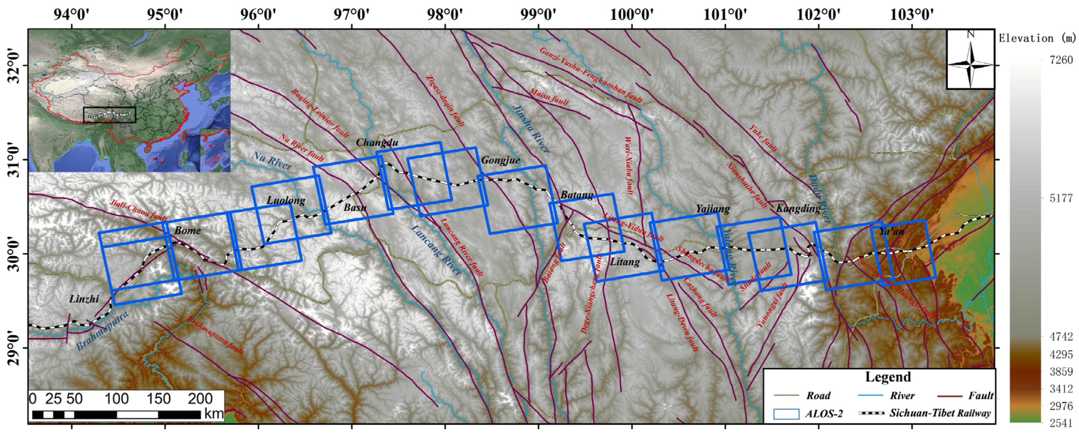
The Linzhi–Ya’an section is currently under construction as part of the Sichuan–Tibet Railway, and spans from the west edge of the Sichuan Basin to the eastern part of the Qinghai–Tibet Plateau, crossing the Himalayas, Nianqing Tanggula Mountains, and Hengduan Mountains, among other regions, as shown in Figure 1. It demonstrates the following features: (1) the terrain is steep and fluctuates considerably, with an elevation range of 627–5013 m, and is high in the west and low in the east, and alpine valleys are widespread [1]. (2) It passes through Dadu River, Yalong River, Jinsha River, Lancang River, and Nujiang River. Therefore, a dense river distribution leads to a remarkable cutting effect [15]. (3) The climate along the route transits from a temperate monsoon climate to a plateau alpine climate, which can be divided into six climate types: subtropical humid climate zone, western Sichuan plateau temperate humid climate zone, eastern Tibet plateau temperate semi-humid climate zone, southeast Tibet subtropical mountainous humid climate zone, southern Qiangtang plateau subtropical semi-arid climate zone, and southern Tibet plateau temperate semi-arid climate zone [16]. The period of rainfall and high temperature is mostly concentrated in summer, which is also a period of high landslide occurrence [17]. (4) The temperature difference between day and night in this region is substantial, and freeze–thaw weathering is extremely strong, which further reduces the stability of the rock mass [18,19]. (5) There are many active faults along the Sichuan–Tibet Railway and the geological tectonic activity is intense. It passes through 24 major faults, such as the Xianshui River, Yushu–Ganzi, Litang–Dewu, Lancang River, Nu River, and Jinsha River faults. Additionally, since the Quaternary, the Indian plate has been subducted and squeezed to the Eurasian plate and the Qinghai–Tibet Plateau has risen rapidly at a rate of 9.5 mm/year; therefore, seismic activity is frequent [20], which constitutes a background for surface deformation in this region. (6) There are substantial stratigraphic differences and weak lithologies along this route; the stratigraphic direction is consistent with the trend of the fault zone. Based on the interaction of the above-mentioned natural characteristics, fractures in the rock mass are widespread, which is conducive to rainwater infiltration [21]. These factors not only lead to frequent landslide disasters, but also induce large-scale, high-level, and long-distance landslides. For example, the Yigong high-level and huge landslide occurred in the year 2000. The sliding time of this landslide lasted for 10 min, and the sliding distance reached 8 km. The Yigong Zangbo River was markedly blocked and the highway was interrupted for several months. It also resulted in large-scale casualties and property losses upstream and downstream [22,23]. In 2018, a large-scale high-level rock landslide occurred in Baige Village, which caused a break in the Jinsha River for 2 days [24]. The economic loss caused by this landslide amounted to CNY 15 billion. Unmanned aerial vehicle (UAV) images of these two landslides are shown in Figure 2. These landslides demonstrated the characteristics of high concealment, rapid sliding speed, long sliding distance, and huge destructive force, which are deemed major challenges for the planning and construction of the Sichuan–Tibet Railway.
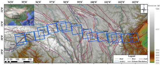
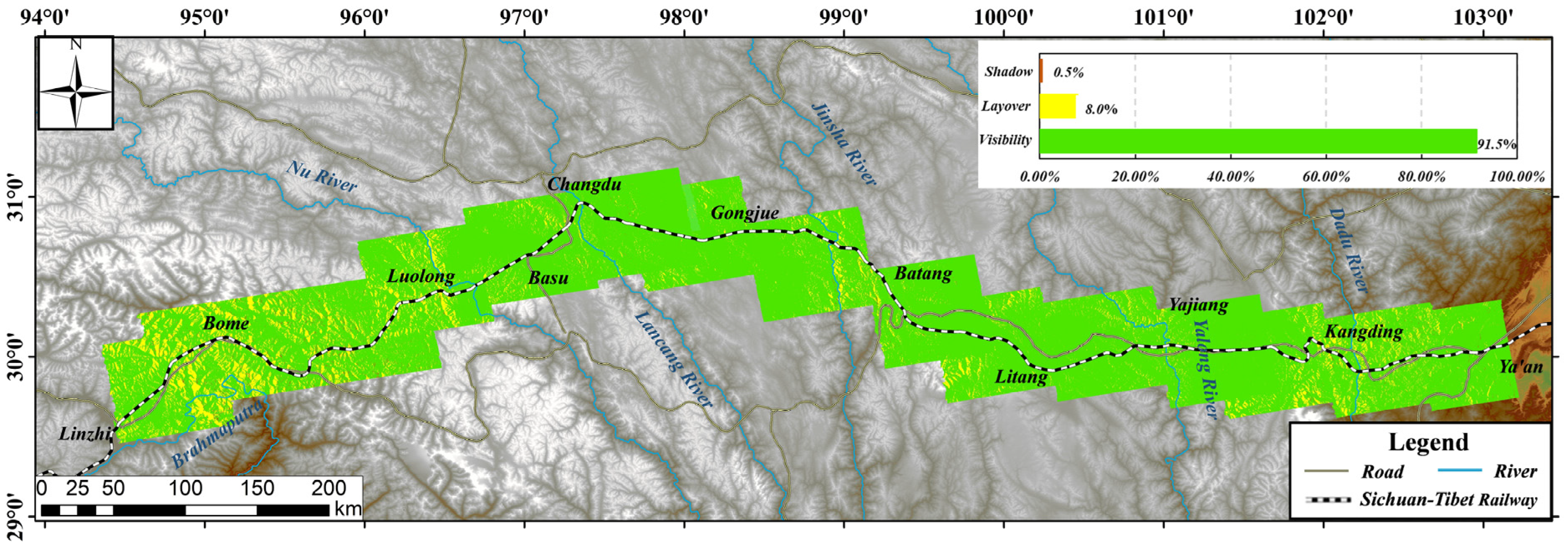
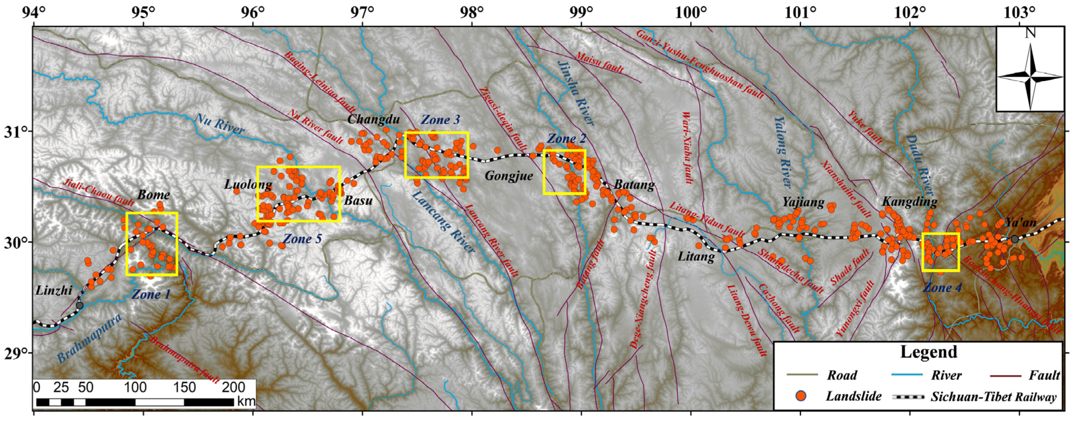
Figure 1.
Study area and synthetic aperture radar (SAR) image coverage. The background is the shaded relief obtained by the shuttle radar topography mission digital elevation model (SRTM DEM). Upper left corner black rectangle indicates the location of the study area in China.
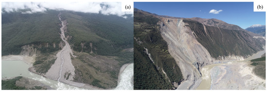
Figure 2.
Unmanned aerial vehicle (UAV) images of typical landslides taken in October 2020. (a) Yigong landslide. (b) Baige landslide.
2.2. Data
To better overcome the decoherence caused by vegetation and ice–snow cover along the railway during InSAR processing, we collected 164 L-band ALOS/PALSAR-2 ascending images, which demonstrate good penetration ability for surface covering, to detect the hidden landslides along the Sichuan–Tibet Railway. Considering the low temporal resolution of ALOS/PALSAR-2 satellite (46 days), the time period of data from 2014 (satellite launching time) to 2020 was selected in this study. The cover range and corresponding parameters of the 16 orbits in the study area are shown in Figure 1 and Table 1, respectively. The visibility, layover, and shadow area of the images were calculated and masked according to the flight parameters of the satellite and external SRTM DEM with a 30-m resolution. Although the research area topography was mostly alpine canyon, according to the overall visibility map of the research area shown in Figure 3, the visibility area accounted for 91.5%, which proved that the selected data could be considered for disaster detection in most study areas. Additionally, SRTM DEM was also used for InSAR data processing.

Table 1.
Parameters of synthetic aperture radar (SAR) satellite images.
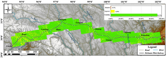
Figure 3.
Visibility analysis map. Green indicates the visibility area, yellow indicates the layover area, and brown indicates the shadow area.
2.3. Methods
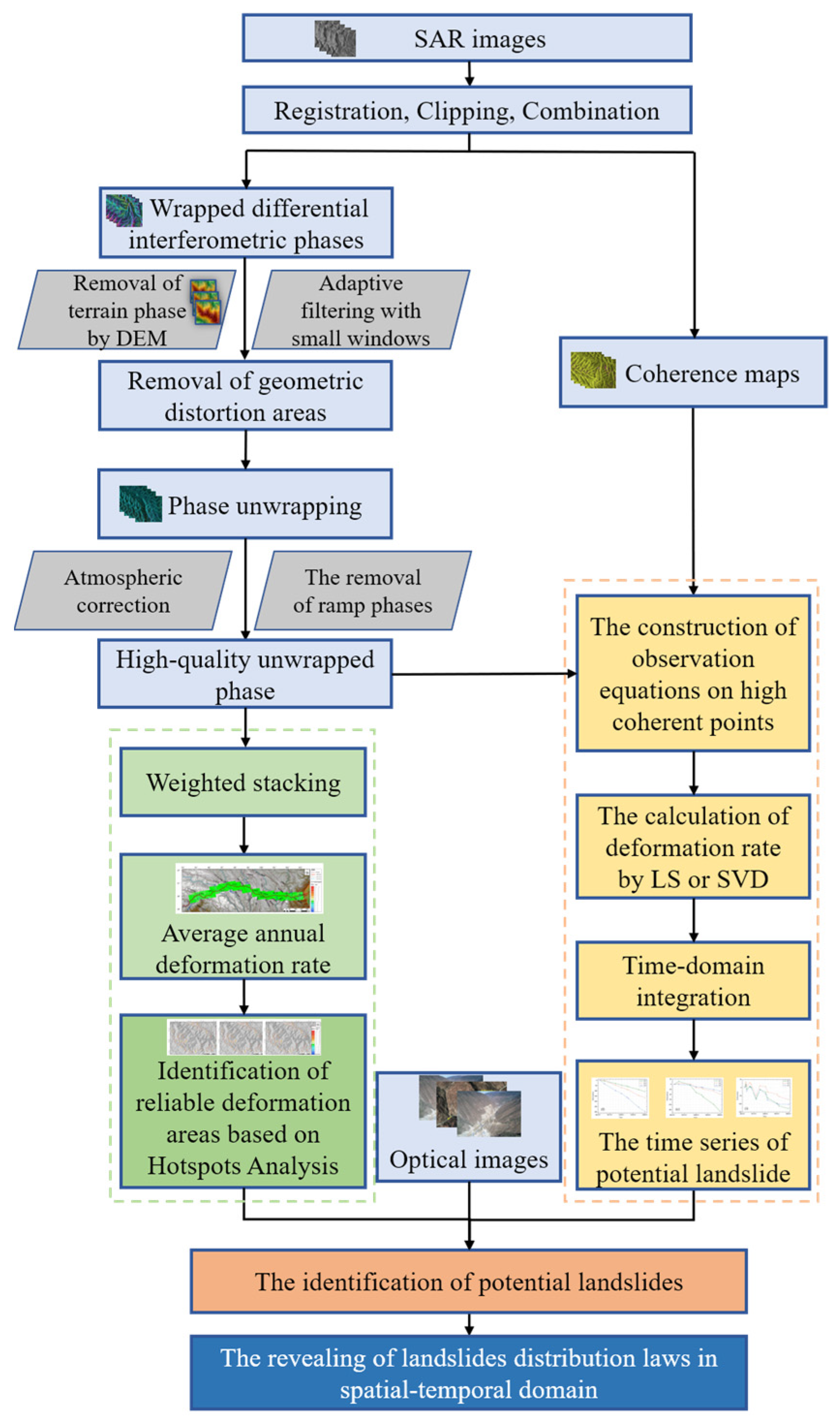
The collected 16-orbit data were preprocessed to obtain single-look complex (SLC) images, and then the combinations of SLC pairs were interfered and unwrapped. Because the terrain along the Sichuan–Tibet Railway fluctuates greatly, the vegetation and ice–snow cover in some areas is serious, and many errors are inevitable during data processing (such as decoherence, atmospheric error and geometric distortion). In this study, errors in the interference and unwrapping process were explored and corrected according to the characteristics of the study area. After selecting high-quality unwrapping maps, the annual deformation rate was calculated based on the stacking-InSAR method. Based on the results, the effective deformation area was directly extracted by the hot spot analysis method. Then, the identification of potential landslides was completed based on effective deformation combined with optical images, geological factors, and time-series deformation methods. Finally, the main controlling factors of landslides were analyzed using a spatial analysis method. A flowchart of the specific method is provided in Figure 4. Detailed methods of stacking, SBAS-InSAR, and hot spot analysis are introduced below.
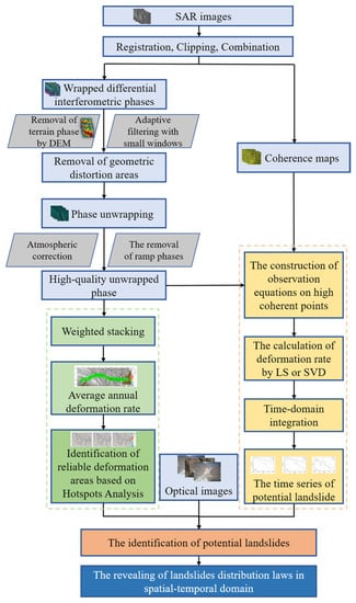
Figure 4.
Flowchart for landslide identification and analysis.
2.3.1. Stacking-InSAR
The stacking-InSAR method can be used in conjunction with the differential interferometric phase after unwrapping to obtain the annual deformation rate. The atmospheric phase error in the superimposed phase can be weakened, which can effectively be used to suppress atmospheric delay and to obtain high-precision deformation monitoring results.
In the present study, interferograms with residual error and low coherence were eliminated, and a certain number of high-quality unwrapping maps were used to obtain the phase deformation rate, as follows [25]:
where represents the weight of the unwrapped phase; the time intervals are considered as the weight, i.e., ; represents the th interference unwrapping phase; and represents the number of interferograms.
2.3.2. SBAS-InSAR
SBAS-InSAR is a short baseline differential interferometry method proposed by Berardino et al. in 2002, which can be used to obtain a continuous deformation time series [26]. This method exhibits a low requirement for SAR data. It also can weaken the influence of decoherence and topographic changes by controlling the time and spatial baselines [27].
In the present study, all SAR images were divided into different short baseline subsets according to a certain time and spatial threshold, and then each combinatorial pair was subjected to interference. After interference processing, the minimum cost flow (MCF) unwrapping method was used for phase unwrapping [28,29], and the observation equation was established, combined with high coherence points. Finally, the least square (LS) or singular value decomposition (SVD) method was used to obtain the minimum norm solution of the velocity vector, and the cumulative deformation of each time period could be obtained by integration in the time domain [26]. To overcome the spatial–temporal decorrelation and consider the low temporal resolution of ALOS-2 data, the temporal and spatial baseline thresholds were set as 500 d and ±700 m, respectively, to obtain more interferograms. Owing to the influence of satellite geometric parameters and terrain factors, the shortened, layover, and shadow errors result in the distortion of SAR images during the detection process [30], a phenomenon which affects the registration of SAR images and leads to the generation of certain noise areas. In the present study, the geometric parameters of satellites and DEM data were used to calculate and effectively remove the shadows and layover areas in the GAMMA software. The error areas could be eliminated, and the accuracy of the interferograms was improved. We also introduced the SRTM DEM data to remove the terrain phase. The adaptive filtering method was used to remove the noise existing in the interferograms [31]. Notably, during filtering, a small filtering window (32 or 16) was selected to avoid excessive information loss. The atmospheric error was corrected by adopting the empirical linear model constructed between the InSAR phase and elevation [32]. In short, the errors were corrected in different situations to obtain the optimal deformation results during data processing.
2.3.3. Automatic Extraction of Effective Deformation Data via Hot Spot Analysis
As the spatial range of the deformation rate is markedly considerable, and as few discrete error deformation points remain, direct landslide identification is deemed time-consuming and laborious. Therefore, this study introduced a hot spot analysis method for large-scale landslide detection. Through the spatial statistical analysis of the obtained large-scale deformation values, the high and low points with evident clustering properties in space were obtained.
The hot spot statistical method used in the study was the Getis−Ord method. statistics is a method used to monitor whether the feature points possess significant spatial clustering properties by checking each element in the adjacent element environment within a certain distance [33,34]. The calculation formula is as follows:
where represents the spatial weight matrix; represents the total number of elements; and x represents the surface displacement recorded by InSAR. Assuming that obeys laws of normal distribution, the Z score of each element point can be calculated using Equation (3); the higher the Z score, the more evident the spatial clustering properties. The following equation is considered:
Among them, represents the variance of , represents the expectation. In the present study, (confidence level is 99%) and of the deformation point was a reliable deformation with evident spatial clustering properties, and was considered the significance level in the hypothesis test.
3. Results and Analyses
3.1. Deformation Rate Map Acquired via InSAR
Annual line of sight (LOS) deformation rate maps of the Ya’an–Linzhi railway section were generated using the stacking-InSAR method, as shown in Figure 5. The region showing an annual deformation rate value of <±10 mm was considered a stable region (represented by using green in Figure 5). Notably, the negative values (represented by using red) indicated that the surface moved away from the satellite, whereas the positive values (represented by using blue) indicated that the surface moved toward the satellite sensor (Figure 5) [35]. It could be inferred that the coherence of the Ya’an–Kangding and Luolong–Linzhi sections was relatively low compared to other regions, which might have been caused by the complex environment [36,37]. Meanwhile, according to the annual deformation rate map, we found that large-scale errors (such as atmospheric and unwrapping errors) could be effectively removed. The spatial landslide distribution was uneven; there were more deformation regions in the east and west, whereas the middle part was relatively stable. Additionally, most deformation regions were distributed along expansive rivers.
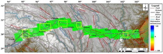
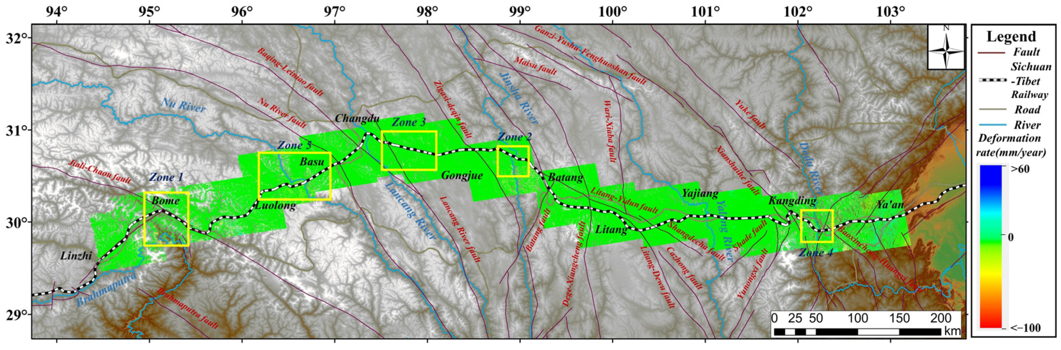
Figure 5.
Annual LOS deformation rate maps calculated by using synthetic aperture radar (SAR) data. The yellow rectangle represents a dense area of large-scale landslides.
3.2. Landslide Deformation Rate Map Obtained via Hot Spot Analysis
Based on the annual deformation rate map obtained by InSAR, a hot spot analysis was performed to automatically extract the effective deformation area. In the present study, five areas with a dense distribution of large-scale landslides were selected for illustration in Figure 6 (note: the locations are shown as yellow rectangles in Figure 5). It could be inferred from Figure 6 that the stable area and the discrete noise points removed after conduction of the hot spot analysis were related to the original deformation rate map, and that only data on the effective deformation area remained. These effective deformation points were more prominent [33], which could markedly be considered to reduce the difficulties of landslide interpretation and rapid identification of landslide hazards.
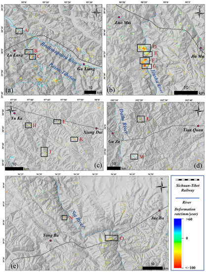
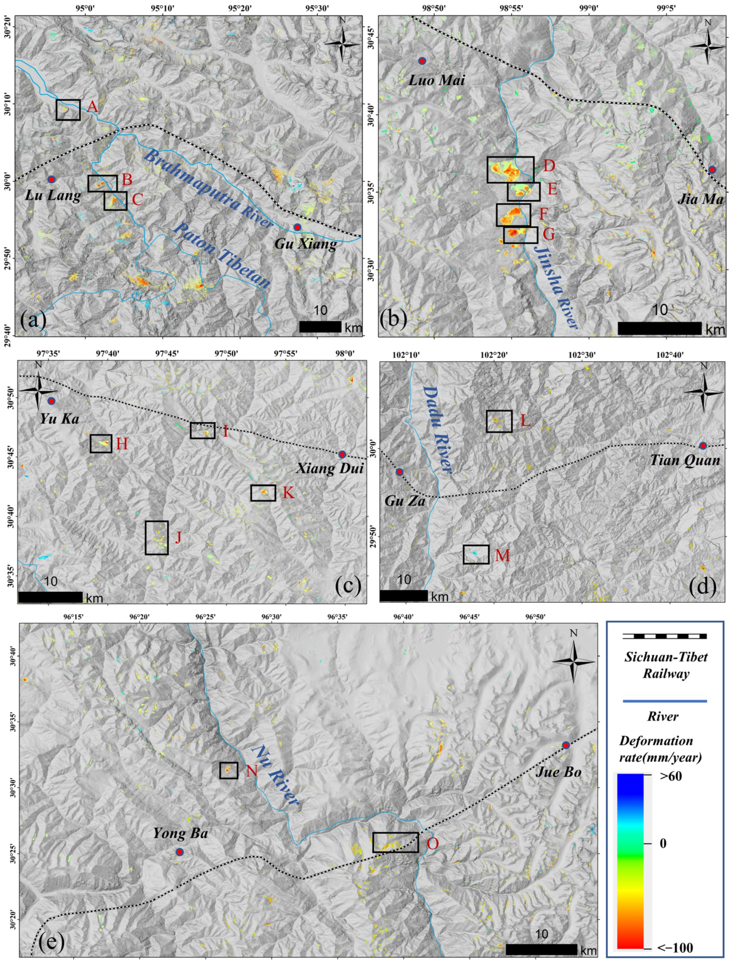
Figure 6.
Hot spot analysis results of key regions. (a) Lulang–Guxiang section, (b) Luomai–Jiama section, (c) Yuka–Xiangdui section, (d) Guza–Tianquan section, and (e) Yongba–Juebo section, corresponding to zones 1–5 in Figure 5, respectively.
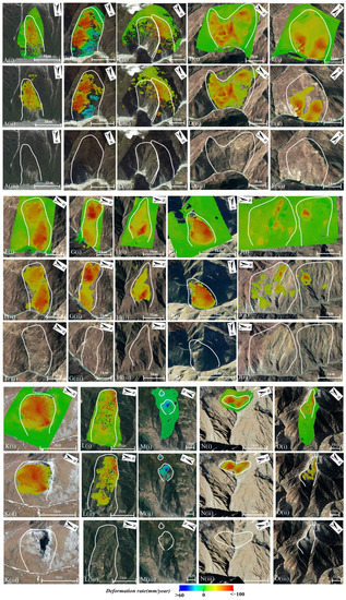
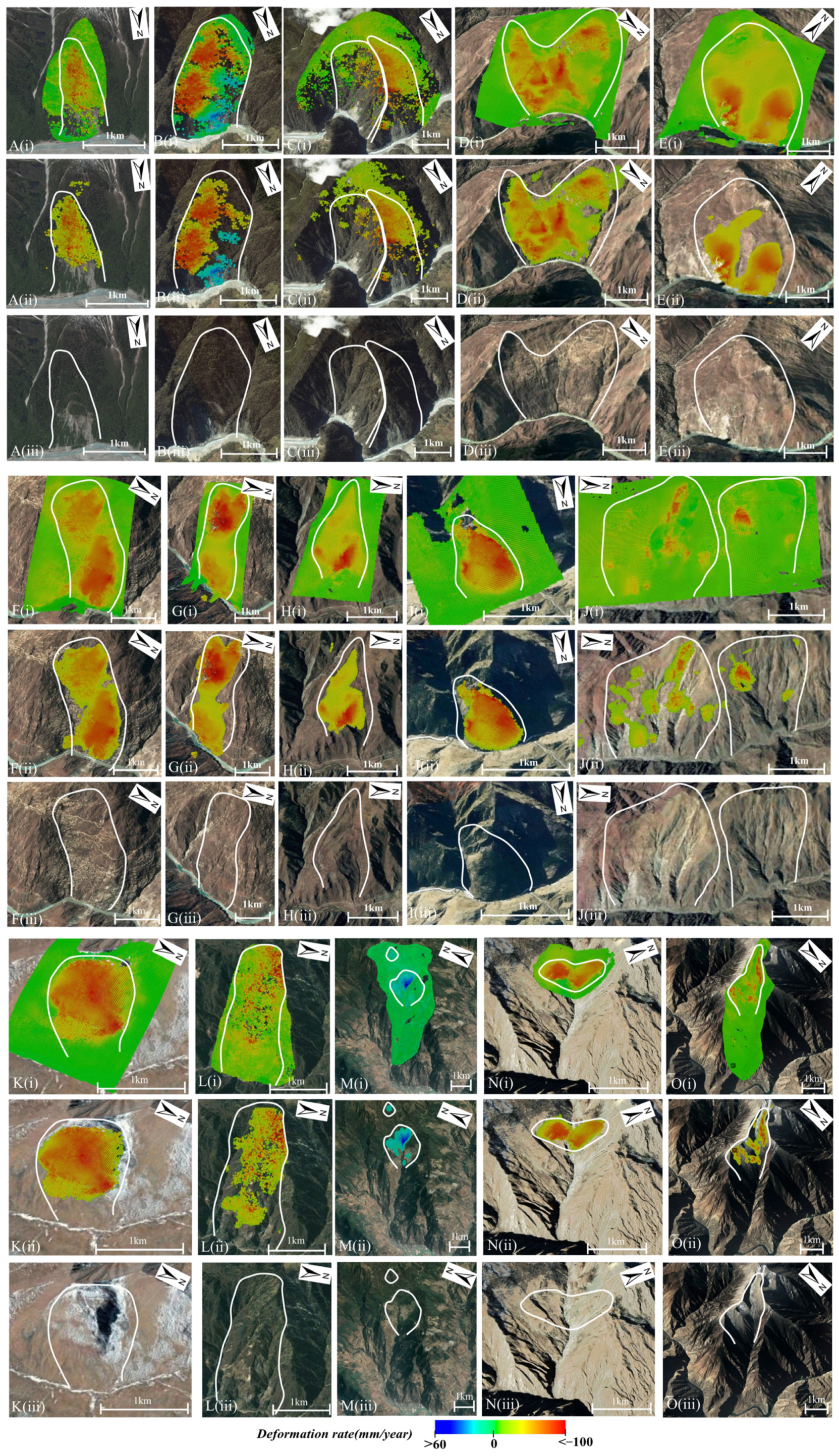
To further illustrate the landslide mapping results, Figure 7 has been depicted, which shows the original results, hot spot analysis results, and optical images of 17 typical large-scale landslides in the key area. The specific locations of the landslide points are shown in Figure 6. By comparing the results, we found that the hot spot analysis could be performed to effectively eliminate the error area, and that the extracted landslide boundary was in good agreement with the optical image. It could also be inferred that some detected landslides were not easily distinguished on optical images because of their high concealment characteristics. However, the landslide could be identified by InSAR, which showed that the InSAR method could not only be used to identify landslides with evident deformation in optical images, but also be used to identify deformed landslides with no remarkable characteristics on optical images. Particularly, the hot spot analysis method can be used to determine the real hidden dangers posed by potential landslides and to provide scientific support for railway planning and construction.
3.3. Active Landslide Inventory
In addition to landslides, large-scale disasters, such as ice collapse, glacier lake outburst, and debris flow, also occurred due to the complex geological and geomorphological conditions along the Sichuan–Tibet Railway. Therefore, landslide disasters must be selected by considering reliable surface deformation data that strictly include information based on geological factors, such as DEM and slope aspect. Furthermore, we mainly identified landslides that posed a threat to the construction of tunnels and bridges within 100 km, and did not consider small landslides and disasters that posed no threat to the railway, such as small collapses and landslides along the river banks. Based on the annual deformation rate after conduction of hot spot analysis, 517 landslides with evident deformation and certain threats to railways were interpreted (Figure 8). Many detected landslides have been validated by field investigation and published articles, such as those pertaining to the Yigong landslide, Lancang River, Jinsha River, and Yalong River landslide groups [11,12,38,39,40,41,42]. By comparing the identification results of hot spot analysis and traditional manual visual interpretation, it was found that traditional visual interpretation resulted in the exclusion of data on 178 missed landslides and 58 misjudged landslides. This finding proves that hot spot analysis can be performed to solve the problem of unintentional exclusion of missed and misjudged landslides during identification to a considerable extent.

Figure 8.
Inventory map of active landslides along the Sichuan–Tibet Railway.
Landslide analysis showed that the overall spatial landslide distribution was uneven, and was relatively dense in Luolong–Basu, Changdu–Tuoba, Jinsha River coast, and Kangding–Ya’an, wherein a total of 358 landslides were identified, accounting for 69.2% of the total number of landslides. It could be inferred from Figure 5 and Figure 8 that the large-scale landslides were mainly concentrated in Lulang–Guxiang, Yuka–Xiangdui, Yongba–Juebo, Jinsha River coast, and Guza–Tianquan County. The large-scale landslides in the Lulang–Guxiang section (Figure 6a) mainly developed along the Palalung Zangbo River. The river flow rate in this area is high and annual runoff can reach 700 m3/s [15]. River erosion, significant tectonic activities, and freeze–thaw weathering are the main triggering factors for the frequent occurrence of landslides in this area [4]. Moreover, the annual deformation rate of most landslides is >100 mm/year and the volume is >1 km2. For example, the famous Yigong landslide occurred along the Palalung Zangbo River [22,23]. Regarding the coastal area of the Jinsha River (Figure 6b), several large-scale landslides were distributed in this area and the deformation rates of these slopes were all >100 mm/year, with a maximum of 180 mm/year. This area presents with substantial terrain fluctuations, evident differences in rainfall, extremely complex climate, and low vegetation coverage [4]. It is also located through four north–south fault zones, and tectonic activity is strong, factors which collectively result in the breakage of the slope and frequent occurrence of landslides. The Yuka–Xiangdui area (Figure 6c) is mainly affected by glaciers, weathering, and crustal uplift, which collectively lead to the wide distribution of the loose deposits and bare bedrock, resulting in the occurrence of large-scale landslides [5]. The Guza–Tianquan section (Figure 6d) belongs to the eastern edge of the Sichuan–Tibet line and is exposed to strong fault and earthquake activities. Therefore, numerous landslides have occurred in this region. The Yongba–Juebo section (Figure 6e) is strongly subjected to erosion and is cut by the Nujiang River. The ice–snow cover area is large and is affected by the subtropical warm and humid climate, and the freeze–thaw effect is remarkable. Landslides occur relatively easily in this environment. Generally, these five sections warrant attention, with a focus on continuous deformation monitoring. In addition, the inventory of 17 typical landslides marked in Figure 6 and Figure 7, which may pose a great threat to railway construction, is shown in Appendix A, Table A1.
3.4. Time-Series Monitoring for Typical Landslides
Based on the landslide identification results, certain high-risk landslides can be monitored using time-series deformation. Therefore, we selected two landslide bodies, G and H, as shown in Figure 9, both of which demonstrate an evident continuous deformation trend. As shown in Figure 9b, the maximum cumulative deformation of landslide G reaches −400 mm, and a continuous deformation trend exists at all three points. This landslide is located on the right bank of the Jinsha River, and there are multiple tensile cracks in the back edge of the slope, and findings indicate that the range of cracks gradually expands with the continuous increase in deformation. Therefore, human activities on the slope, river cuts, and rainfall may cause failure of this slope. If sliding occurs, it may block the Jinsha River and endanger the upstream bridge, a phenomenon which may also induce failure of other unstable slopes and may expand the scale of damage. Therefore, continuous monitoring is recommended in the future. Landslide H is an old landslide, and there is less vegetation cover on this slope. Optical imaging results reveal that it is a freeze–thaw landslide. According to the time-series deformation of this landslide, the maximum cumulative deformation of P3 on this landslide can reach −296 mm (Figure 9d), and the three points demonstrate a state of continuous deformation, a phenomenon which will also pose a grave threat to the construction and operation of nearby buildings and structures. It could be inferred from the time-series deformation of these two disaster points that although ALOS-2 data exhibited certain disadvantages in terms of time resolution, the overall cumulative deformation trend could also be studied appropriately; therefore, such landslides can be monitored effectively by considering InSAR time-series deformation.
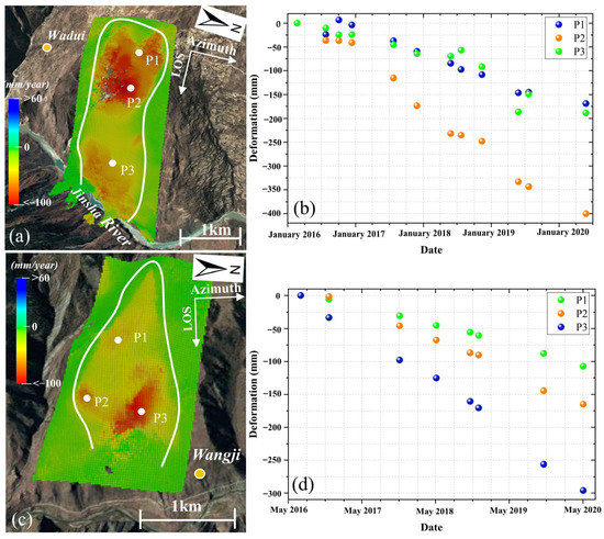
Figure 9.
Deformation rates and time-series deformation of typical landslides. (a) Annual deformation rate of landslide G. (b) Time-series deformation of landslide G; points P1, P2, and P3 are marked in (a). (c) Annual deformation rate of landslide H. (d) Time-series deformation of landslide H; points P1, P2, and P3 are marked in (c). Locations of landslides G and H are shown in Figure 6.
4. Discussion
4.1. Effectiveness of the Hot Spot Analysis Method
To verify the effectiveness of hot spot analysis, we considered the annual deformation rate containing many error regions as an example to explore the performance of hot spot analysis in extracting effective deformation. This area is located in Tianquan County and many errors exist in the annual deformation rate, owing to the high vegetation coverage. Figure 10a shows the original annual deformation rate. Figure 10b shows the deformation area obtained only by removing data on the stable region from Figure 10a using a deformation threshold, which contained many discontinuous deformation points. Interpretation of landslides directly from the information presented in Figure 10a,b is difficult. Figure 10c shows the results of extracting data on the effective deformation area by hot spot analysis. It could be inferred that most error points were eliminated and the effective deformation area was remarkably clear; thus, landslide interpretation could be performed rapidly and accurately, whereby data on 15 effective landslide areas were effectively extracted in this area (Figure 10c). Figure 10d shows the difference between Figure 10b,c, which indicates the error deformation area removed via hot spot analysis. It could be inferred that the hot spot analysis could be performed to remove many discrete and invalid deformation points that caused significant interference to interpretation.
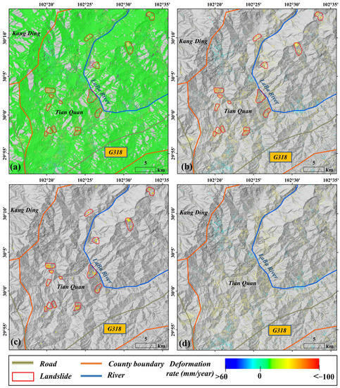
Figure 10.
Comparison between original annual deformation rate map, stable region data removing results, and hot spot analysis results. (a) Original annual deformation rate. (b) Annual deformation rate map after removing data on stable region by considering deformation threshold. (c) Annual deformation rate map after hot spot analysis. (d) Error deformation area removed by hot spot analysis.
4.2. Controlling Factors of Spatial Landslide Distribution
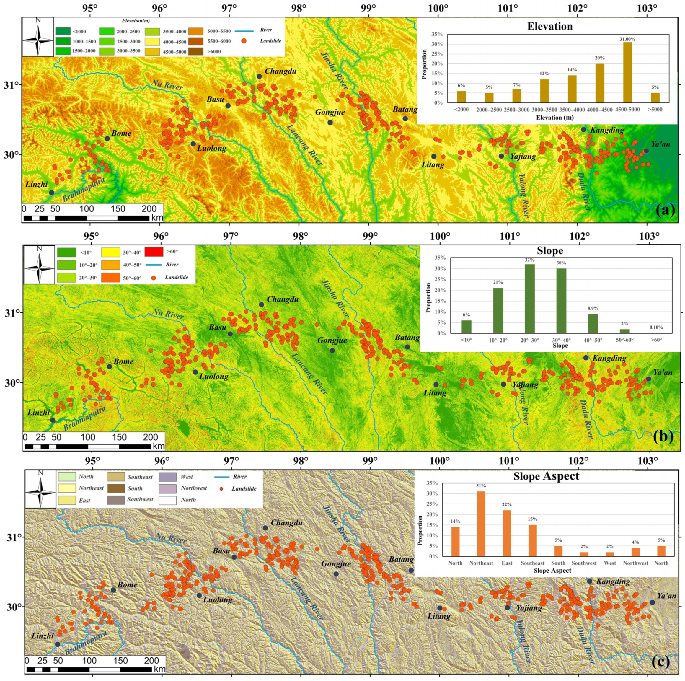
To determine the main factors controlling the spatial landslide distribution along the Sichuan–Tibet Railway, the elevation, slope, aspect, river, fault zone, seismic peak acceleration, and rainfall were selected and their relationships with the spatial landslide distribution were analyzed. In the vertical direction, the relationships between landslide and elevation, slope, and aspect were analyzed using spatial analysis statistical tools. As shown in Figure 11a, landslide disasters gradually increased with an increase in elevation, and decreased markedly when the elevation exceeded 5000 m. Therefore, elevation is an important factor affecting spatial landslide distribution [43]. Additionally, 77% of the landslide hazard points were located at altitudes ranging from 3000–5000 m. Figure 11b depicts the relationship between the landslide points and the slope. It could be inferred that a high slope almost developed along the rivers. Statistical analysis showed that 81% of the landslides were distributed on slopes of 10–40°. The reason for this phenomenon is that low slopes do not present with sufficiently dynamic conditions, and high slopes are not conducive to the accumulation of landslide materials [44]. Therefore, the slope in the middle was beneficial for the occurrence of landslides. Furthermore, the terrain slope affects the rainfall and heat distribution, thereby affecting vegetation coverage. Figure 11c illustrates the relationship between landslides and the slope aspect. According to the statistical diagram, it could be inferred that the landslides were mostly developed in the northeastern and eastern areas, accounting for 53% of the total landslides. This may be attributable to the presence of less sunshine in these two directions, underdeveloped vegetation, and poor slope stability, thereby rendering these areas more prone to landslides [45].
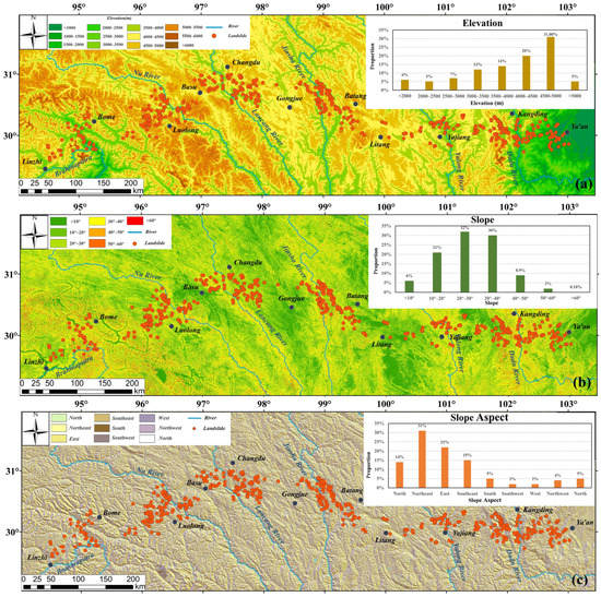
Figure 11.
Relationships between vertical geological factors and landslides. Relationships between (a) elevation and spatial landslide distribution; (b) slope and spatial landslide distribution; and (c) aspect and spatial landslide distribution. The statistical charts of each factor are displayed in the upper-right corner in each map.
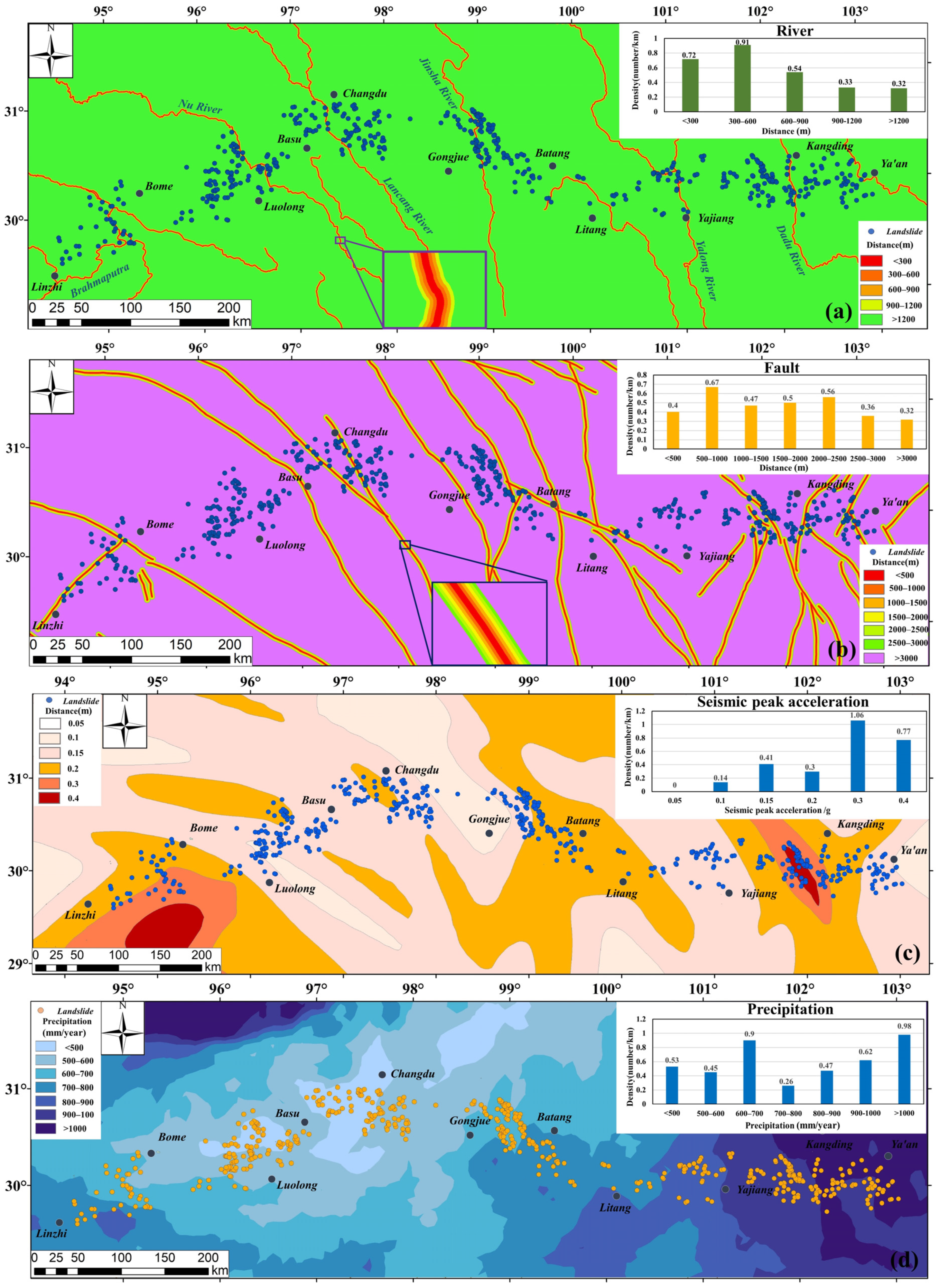
In the horizontal direction, the relationships between landslides and fault zone, seismic peak acceleration, and rainfall were statistically analyzed. There are many rivers present along the line, and river cutting and lateral erosion seriously affect the slope stability. After seven buffer zones were created on the river, the relationship between the spatial landslide distribution and the distance from the river was analyzed. The number of landslides decreased with an increased distance from the river (Figure 12a), and the highest landslide density was observed to be in the area 300–600 m from the river (i.e., 0.91 landslides/km). Meanwhile, these areas are considered more suitable for human habitation; therefore, they have also demonstrated vulnerability due to human activities [43]. In general, there are close relationships between rivers and landslides. The fault zone changes the rock mass structure and causes crushing, which is conducive to rainwater infiltration and induces natural disasters. Figure 12b shows the statistical analysis of the distance between the landslide points and the fault zone. The number of landslides showed a slowly decreasing trend, with an increase in the distance between the landslide and the fault zone, a finding which was consistent with the theory and proved that the fault zone exerted a certain influence on landslide development. As one of the main triggering factors of landslides, earthquakes can not only directly induce landslide failure, but can also reduce the threshold of landslide failure by reducing slope stability [20,46]. Figure 12c shows that the landslide density reached a substantial value when the seismic peak acceleration was 0.3 g and 0.4 g, a finding which proved that it affected the spatial landslide distribution. Precipitation is another important factor inducing landslides [47]. In this study, information on annual average precipitation (GPM) [48] from 2016–2021 was used to explore the relationship between landslides and precipitation. It could be inferred from Figure 12d that rainfall was more distributed in the east and less in the west. When the rainfall was >700 mm/year, the landslide density gradually increased with increasing rainfall. When it reached a value >1000 mm/year, the landslide density reached a maximum of 0.98 landslides/km. When the rainfall was <700 mm/year, it exerted minimal effect on landslide development, and the landslide in the region was dominated by other factors; therefore, there were no evident statistical relationships with rainfall. In general, in the horizontal direction, the seismic peak acceleration, rainfall, river, and fault zone correlated with the landslide density, which largely determined the spatial landslide distribution along the Sichuan–Tibet Railway.
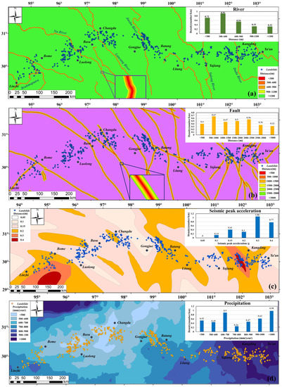
Figure 12.
Relationships between horizontal geological factors and landslides. Relationships between (a) river and spatial landslide distribution; (b) fault zone and spatial landslide distribution; (c) seismic peak acceleration and spatial landslide distribution; and (d) precipitation and spatial landslide distribution. The statistical charts of each factor are displayed in the upper-right corner in each map.
The above-mentioned analysis shows that landslides along the Sichuan–Tibet Railway are mainly affected by the following factors: (1) the river erosion cutting and river cutting will render the slope steep and unstable; therefore, most landslides in the region are affected by this factor and mainly occur on both sides of the river. (2) Fault zones and earthquakes: there are many fault zones along the Sichuan–Tibet Railway, and seismic activity is frequent. These activities destroy the integrity of the rock mass, enable easy infiltration of the rainwater, and lead to the production of a weak sliding surface, resulting in the occurrence of landslides. Especially in the east, landslides are concentrated near the Baqing–Leiniaoqi, Lancang River, Batang, Xianshui River, and Wenchuan–Maowen fault zones. (3) Change in freeze–thaw: the analysis shows that landslides may occur frequently at elevations of 3000–5000 m. The temperature difference between day and night is considerable, and repeated freezing and thawing may weaken the slope integrity. (4) Precipitation: owing to the simultaneous rainfall and heat along the line, extreme precipitation is common [49], and ice–snow melting water and rainfall will increase the slope weight and sliding force, phenomena which will also lead to the occurrence of landslides.
5. Conclusions
In the present study, using multi-temporal InSAR methods and 164 scenes of ALOS-2 ascending data, preliminary detection of landslide hazards in the Linzhi–Ya’an section of the Sichuan–Tibet Railway was conducted. After obtaining the annual deformation rate, the hot spot analysis method was introduced to rapidly extract data on the effective deformation. Then, the optical images and other geological factors were combined for landslide interpretation. A total of 517 landslide points were detected, which posed a certain threat to railway construction and safe operation. Large-scale landslides were mainly concentrated in Lulang–Guxiang, Yuka–Xiangdui, Yongba–Juebo, Jinsha River coast, and Guza–Tianquan County. By comparing the results of the original InSAR and the hot spot analysis, it was found that the hot spot analysis method could be applied to extract data on the effective deformation area, which considerably improved the speed of visual interpretation. Most importantly, it reduced the number of misjudgments and missing judgments to a certain extent. Finally, according to the detection results of landslides, the correlations between spatial landslide distribution and geological factors (such as slope, aspect, elevation, fault zone, river, and precipitation) were explored. The spatial landslide distribution was strongly and positively correlated with the distance between rivers and fault zones, and the main influencing factors were rainfall, river, freeze–thaw weathering, and earthquakes. This study provides important information that may be considered as vital technical support for the construction and safe operation of the Linzhi–Ya’an section of the Sichuan–Tibet Railway. Although the reliability of the hot spot analysis method has been proved in this study, it is limited by the determination of distance and stable deformation thresholds. Generally, these two thresholds are defined by human experience, which may result in the missing judgments of efficient deformation. Thus, accurate determination of distance and stable deformation thresholds will be studied in our subsequent research.
Author Contributions
Conceptualization, J.Z. and W.Z.; methodology, W.Z.; validation, J.Z., W.Z., Y.C. and Z.L.; formal analysis, J.Z. and W.Z.; investigation, J.Z. and Y.C.; resources, W.Z. and Z.L.; data curation, J.Z.; writing—original draft preparation, J.Z.; writing—review and editing, J.Z. and W.Z.; visualization, J.Z.; supervision, J.Z. and W.Z.; project administration, W.Z. and Z.L.; funding acquisition, Z.L. All authors have read and agreed to the published version of the manuscript.
Funding
This work was supported by the Natural Science Foundation of China (Nos. 41941019, 42074040, 41731066, and 41790445), the National Key R&D Program of China (Nos. 2020YFC1512001, 2019YFC1509800), and China Geological Survey project (No. DD20190647).
Institutional Review Board Statement
Not applicable.
Informed Consent Statement
Not applicable.
Data Availability Statement
The ALOS/PALSAR-2 data used in this study were provided by JAXA, Japan, https://auig2.jaxa.jp/ips/home (accessed on 21 May 2021); and the one arc-second SRTM DEM was freely downloaded from the website https://e4ftl01.cr.usgs.gov/MEASURES/SRTMGL1.003/2000.02.11/ (accessed on 21 May 2021).
Acknowledgments
The figures in this study were prepared using ArcGIS, Matlab 2019a and Origin. We thank the editor and four reviewers for their insightful suggestions to this article. We also thank the Google Earth Platform for providing the optical remote sensing images.
Conflicts of Interest
The authors declare no conflict of interest.
Appendix A
Table A1.
Detailed information of 17 typical landslides.
Table A1.
Detailed information of 17 typical landslides.
| No | Name | Longitude (°) | Latitude (°) | Length (km) | Width (km) | Distance from Railway (km) | Level of Impact | |
|---|---|---|---|---|---|---|---|---|
| A | Famudui | 94.95368 | 30.15536 | 2.56 | 1.36 | −68 | 9.2 | High |
| B | Bengyibaqu | 95.03041 | 29.99601 | 3.08 | 1.30 | −112 | 8.7 | High |
| C-1 | Ruodelong-1 | 95.06279 | 29.94954 | 2.85 | 2.57 | −116 | 13.2 | Medium |
| C-2 | Ruodelong-2 | 96.06550 | 29.96675 | 3.32 | 1.66 | −129 | 13.9 | Medium |
| D | Xiongba | 98.91216 | 30.60672 | 2.86 | 3.95 | −102 | 8.5 | High |
| E | Sela | 98.92901 | 30.58451 | 1.73 | 2.32 | −78 | 10.9 | High |
| F | Gongba | 98.91872 | 30.55925 | 3.04 | 1.35 | −105 | 13.6 | High |
| G | Guoba | 98.92528 | 30.54212 | 2.33 | 1.04 | −137 | 15.4 | High |
| H | Baojiang | 97.66345 | 30.76913 | 1.67 | 1.79 | −90 | 6.5 | Medium |
| I | Kaqu | 97.80549 | 30.78462 | 0.93 | 0.62 | −67 | 1.1 | High |
| J-1 | Yongqu-1 | 97.74240 | 30.62914 | 2.83 | 1.57 | −72 | 16.2 | Medium |
| J-2 | Yongqu-2 | 97.73941 | 30.64867 | 2.52 | 1.49 | −73 | 15.6 | Medium |
| K | Laxipu | 97.88711 | 30.70119 | 1.09 | 0.90 | −65 | 8.4 | Medium |
| L | Xinjinggou | 102.34174 | 30.05203 | 2.43 | 1.15 | −112 | 13.1 | Medium |
| M | Haiziping | 102.29715 | 29.80276 | 1.58 | 1.05 | 69 | 12.9 | Medium |
| N | Kuona | 96.44392 | 30.52347 | 0.88 | 1.28 | −85 | 12.2 | Medium |
| O | Keji | 96.65205 | 30.42871 | 3.85 | 1.44 | −88 | 0.8 | High |
C-1/2 and J-1/2 represent the landslide on the left and right sides in Figure 7C; represents the maximum deformation rate for landslide with unit of mm/year; Level of impact is the estimated based on the landslide deformation, size, and distance to railway.
References
- Peng, J.B.; Cui, P.; Zhuang, J.Q. Challenges to engineering geology of Sichuan—Tibet railway. Chin. J. Rock Mech. Eng. 2020, 39, 2377–2389. (In Chinese) [Google Scholar]
- Zhang, G.Z.; Jiang, L.W.; Song, Z.; Wu, G. Research on the Mountain Disaster and Geological Alignment Fundamental of Sichuan-Tibet Railway Running Through N-S Mountain Area. J. Railw. Eng. Soc. 2016, 33, 21–24. (In Chinese) [Google Scholar]
- Xue, Y.G.; Kong, F.M.; Yang, W.M.; Qiu, D.H.; Su, M.S.; Fu, K.; Ma, X.M. Main unfavorable geological conditions and engineering geological problems along Sichuan-Tibet railway. Chin. J. Rock Mech. Eng. 2020, 39, 445–468. (In Chinese) [Google Scholar]
- Guo, C.B.; Zhang, Y.S.; Jiang, L.W.; Shi, J.S.; Meng, W.; Du, Y.B.; Ma, C.T. Discussion on the Environmental and Engineering Geological Problems along the Sichuan-Tibet Railway and Its Adjacent Area. J. Geosci. 2017, 31, 887. (In Chinese) [Google Scholar]
- Li, X.Z.; Cui, Y.; Zhang, X.G.; Zhong, W.; Bian, J.H.; Huang, S.W.; Xu, R.C. Types, Characteristics and Spatial Distribution and Development of Collapse and Sliding Disaster in Sichuan-Tibet Railway. C. Natl. Annu. Meet. Eng. Geol. 2019, 27, 110–120. (In Chinese) [Google Scholar]
- Zhao, C.Y.; Zhang, Q.; Yin, Y.P.; Lu, Z.; Yang, C.S.; Zhu, W.; Li, B. Pre-, co-, and post-rockslide analysis with ALOS/PALSAR imagery: A case study of the Jiweishan rockslide, China. Nat. Hazards Earth Syst. Sci. 2013, 13, 2851–2861. [Google Scholar] [CrossRef] [Green Version]
- Raspini, F.; Ciampalini, A.; Conte, S.D.; Lombardi, L.; Nocentini, M.; Gigli, G.; Ferretti, A.; Casagli, N. Exploitation of amplitude and phase of satellite SAR images for landslide mapping: The case of Montescaglioso (South Italy). Remote Sens. 2015, 7, 14576–14596. [Google Scholar] [CrossRef] [Green Version]
- Zhao, C.Y.; Lu, Z.; Zhang, Q.; Fuente, J.D.L. Large-area landslide detection and monitoring with ALOS/PALSAR imagery data over Northern California and Southern Oregon, USA. Remote Sens. Environ. 2012, 124, 348–359. [Google Scholar] [CrossRef]
- Darwish, N.; Kaiser, M.; Koch, M.; Gaber, A. Assessing the Accuracy of ALOS/PALSAR-2 and Sentinel-1 Radar Images in Estimating the Land Subsidence of Coastal Areas: A Case Study in Alexandria City, Egypt. Remote Sens. 2021, 13, 1838. [Google Scholar] [CrossRef]
- Zhang, L.; Liao, M.S.; Dong, J.; Xu, Q.; Gong, J.Y. Early Detection of Landslide Hazards in Mountainous Areas of West China Using Time Series SAR Interferometry-A Case Study of Danba, Sichuan. J. Geomat. Inf. Sci. Wuhan Univ. 2018, 43, 2039–2049. (In Chinese) [Google Scholar]
- Liu, X.J.; Zhao, C.Y.; Zhang, Q.; Lu, Z.; Liu, C. Integration of Sentinel-1 and ALOS/PALSAR-2 SAR datasets for mapping active landslides along the Jinsha River corridor, China. J. Eng. Geol. 2021, 284, 106033. [Google Scholar] [CrossRef]
- Zhang, J.J.; Gao, B.; Liu, J.K.; Chen, L.; Huang, H.; Li, J. Early Landslide Detection in the Lancangjiang Region along the Sichuan-Tibet Railway Based on SBAS-InSAR Technology. Geoscience 2020, 35, 64–73. (In Chinese) [Google Scholar]
- Golshani, P.; Maghsoudi, Y.; Sohrabi, H. Relating ALOS-2 PALSAR-2 Parameters to Biomass and Structure of Temperate Broadleaf Hyrcanian Forests. Indian Soc. Remote Sens. J. 2019, 47, 749–761. [Google Scholar] [CrossRef]
- Dun, J.; Feng, W.; Yi, X.; Zhang, G.; Wu, M. Detection and Mapping of Active Landslides before Impoundment in the Baihetan Reservoir Area (China) Based on the Time-Series InSAR Method. Remote Sens. 2021, 13, 3213. [Google Scholar] [CrossRef]
- Guo, C.B.; Tang, J.; Wu, R.A.; Ren, S.Z. Landslide Susceptibility Assessment Based on WOE Model along Jiacha-Langxian County Section of Sichuan—Tibet Railway, China. J. Mt. Res. 2019, 37, 240–251. (In Chinese) [Google Scholar]
- Chen, C.; Tian, L.; Zhu, L.; Zhou, Y. The Impact of Climate Change on the Surface Albedo over the Qinghai-Tibet Plateau. Remote Sens. 2021, 13, 2336. [Google Scholar] [CrossRef]
- Qiao, B.; Zhu, L.; Yang, R. Temporal-spatial differences in lake water storage changes and their links to climate change throughout the Tibetan Plateau. Remote Sens. Environ. 2019, 222, 232–243. [Google Scholar] [CrossRef]
- Zhang, W.; Wu, J.; Zhan, S.; Pan, B.; Cai, Y. Environmental geochemical characteristics and the provenance of sediments in the catchment of lower reach of Yarlung Tsangpo River, southeast Tibetan Plateau. J. Catena 2021, 200, 105150. [Google Scholar] [CrossRef]
- Yin, G.; Luo, J.; Niu, F.; Zhou, F.; Meng, X.; Lin, Z.; Liu, M. Spatial Analyses and Susceptibility Modeling of Thermokarst Lakes in Permafrost Landscapes along the Qinghai–Tibet Engineering Corridor. Remote Sens. 2021, 13, 1974. [Google Scholar] [CrossRef]
- Wu, J.; Song, X.; Wu, W.; Meng, G.; Ren, Y. Analysis of Crustal Movement and Deformation in Mainland China Based on CMONOC Baseline Time Series. Remote Sens. 2021, 13, 2481. [Google Scholar] [CrossRef]
- Zeng, Q.L.; Yuan, G.X.; Mcsaveney, M.; Ma, F.; Wei, R.Q.; Liao, L.; Du, H. Timing and seismic origin of Nixu rock avalanche in southern Tibet and its implications on Nimu active fault. Eng. Geol. 2020, 268, 105522. [Google Scholar] [CrossRef]
- Wu, C.; Hu, K.; Liu, W.; Wang, H.; Zhang, X. Morpho-sedimentary and stratigraphic characteristics of the 2000 Yigong River landslide dam outburst flood deposits, eastern Tibetan Plateau. J. Geomorphol. 2020, 367, 107293. [Google Scholar] [CrossRef]
- Li, J.; Chen, N.; Zhao, Y.; Liu, M.; Wang, W. A catastrophic landslide triggered debris flow in China’s Yigong: Factors, dynamic processes, and tendency. J. Earth Sci. Res. J. 2020, 24, 71–82. [Google Scholar] [CrossRef] [Green Version]
- Li, Y.; Jiao, Q.; Hu, X.; Li, Z.; Ba, R. Detecting the slope movement after the 2018 Baige Landslides based on ground-based and space-borne radar observations. J. Int. J. Appl. Earth Obs. Geoinf. 2020, 84, 101949. [Google Scholar] [CrossRef]
- Lyons, S. Fault creep along the southern San Andreas from interferometric synthetic aperture radar, permanent scatterers, and stacking. J. Geophys. Res. Solid Earth 2003, 108, B1. [Google Scholar] [CrossRef]
- Berardino, P.; Fornaro, G.; Lanari, R.; Sansosti, E. A new algorithm for surface deformation monitoring based on small baseline differential SAR interferograms. IEEE Trans. Geosci. Remote Sens. 2002, 40, 2375–2383. [Google Scholar] [CrossRef] [Green Version]
- Hu, X.; Wang, T.; Pierson, T.C.; Lu, Z.; Kim, J.; Cecere, T.H. Detecting seasonal landslide movement within the Cascade landslide complex (Washington) using time-series SAR imagery. Remote Sens. Environ. 2016, 187, 49–61. [Google Scholar] [CrossRef] [Green Version]
- Costantini, M. A novel phase unwrapping method based on network programming. J. IEEE Trans. Geosci. Remote Sens. 1998, 36, 813–821. [Google Scholar] [CrossRef]
- Pepe, A.; Lanari, R. On the extension of the minimum cost flow algorithm for phase unwrapping of multitemporal differential SAR interferograms. IEEE Trans. Geosci. Remote Sens. 2006, 44, 2374–2383. [Google Scholar] [CrossRef]
- Fuhrmann, T.; Garthwaite, M.C. Resolving Three-Dimensional Surface Motion with InSAR: Constraints from Multi-Geometry Data Fusion. Remote Sens. 2019, 11, 241. [Google Scholar] [CrossRef] [Green Version]
- Goldstein, R.M.; Werner, C.L. Radar interferogram filtering for geophysical applications. J. Geophys. Res. Lett. 1998, 25, 4035–4038. [Google Scholar] [CrossRef] [Green Version]
- Doin, M.P.; Lasserre, C.; Peltzer, G.; Cavalié, O.; Doubre, C. Corrections of stratified tropospheric delays in SAR interferometry: Validation with global atmospheric models. J. Appl. Geophys. 2009, 69, 35–50. [Google Scholar] [CrossRef]
- Getis, A.; Ord, J.K. The analysis of spatial association by use of distance statistics. J. Geogr. Anal. 2010, 24, 127–145. [Google Scholar]
- Getis, A.; Ord, J.K. Local spatial statistics: An overview. In Spatial Analysis: Modelling in a GIS Environment; GeoInformation International: Cambridge, UK, 1996; pp. 261–277. [Google Scholar]
- Bekaert, D.P.; Handwerger, A.L.; Agram, P.; Kirschbaum, D.B. InSAR-based detection method for mapping and monitoring slow-moving landslides in remote regions with steep and mountainous terrain: An application to Nepal. Remote Sens. Environ. 2020, 249, 111983. [Google Scholar] [CrossRef]
- Ma, S.; Xu, C.; Shao, X.; Xu, X.; Liu, A. A Large Old Landslide in Sichuan Province, China: Surface Displacement Monitoring and Potential Instability Assessment. Remote Sens. 2021, 13, 2552. [Google Scholar] [CrossRef]
- Zhang, W.; Zhu, W.; Tian, X.; Zhang, Q.; Zhao, C.; Niu, Y.; Wang, C. Improved DEM Reconstruction Method Based on Multibaseline InSAR. IEEE Geosci. Remote Sens. Lett. 2021, 1–5. [Google Scholar] [CrossRef]
- Peeters, A.; Zude, M.; Käthner, J.; Ünlü, M.; Kanber, R.; Hetzroni, A.; Gebbers, R.; Ben-Gal, A. Getis–Ord’s hot-and cold-spot statistics as a basis for multivariate spatial clustering of orchard tree data. J. Comput. Electron. Agric. 2015, 111, 140–150. [Google Scholar] [CrossRef]
- Zhao, C.; Kang, Y.; Zhang, Q.; Lu, Z.; Li, B. Landslide Identification and Monitoring along the Jinsha River Catchment (Wudongde Reservoir Area), China, Using the InSAR Method. Remote Sens. 2018, 10, 993. [Google Scholar] [CrossRef] [Green Version]
- Qi, S.; Zou, Y.; Wu, F.; Yan, C.; Fan, J.; Zang, M.; Zhang, S.; Wang, R. A Recognition and Geological Model of a Deep-Seated Ancient Landslide at a Reservoir under Construction. Remote Sens. 2017, 9, 383. [Google Scholar] [CrossRef] [Green Version]
- Hao, J.; Wu, T.; Wu, X.; Hu, G.; Zou, D.; Zhu, X.; Zhao, L.; Li, R.; Xie, C.; Ni, J.; et al. Investigation of a Small Landslide in the Qinghai-Tibet Plateau by InSAR and Absolute Deformation Model. Remote Sens. 2019, 11, 2126. [Google Scholar] [CrossRef] [Green Version]
- Lu, H.; Ma, L.; Fu, X.; Liu, C.; Wang, Z.; Tang, M.; Li, N. Landslides Information Extraction Using Object-Oriented Image Analysis Paradigm Based on Deep Learning and Transfer Learning. Remote Sens. 2020, 12, 752. [Google Scholar] [CrossRef] [Green Version]
- Napoli, D.M.; Marsiglia, P.; Martire, D.; Ramondini, M.; Calcaterra, D. Landslide susceptibility assessment of wildfire burnt areas through earth-observation techniques and a machine learning-based approach. Remote Sens. 2020, 12, 2505. [Google Scholar] [CrossRef]
- Kavzoglu, T.; Sahin, E.; Colkesen, I. Landslide susceptibility mapping using GIS-based multi-criteria decision analysis, support vector machines, and logistic regression. J. Landslides 2014, 11, 425–439. [Google Scholar] [CrossRef]
- Wu, Y.; Li, W.; Wang, Q.; Liu, Q.; Yang, D.; Xing, M.; Pei, Y.; Yan, S. Landslide susceptibility assessment using frequency ratio, statistical index and certainty factor models for the Gangu County, China. J. Arab. J. Geosci. 2016, 9, 1–16. [Google Scholar] [CrossRef]
- Wu, C.H.; Cui, P.; Li, Y.S.; Ayala, I.; Huang, C.; Yi, S.J. Seismogenic fault and topography control on the spatial patterns of landslides triggered by the 2017 Jiuzhaigou earthquake. J. Mt. Sci. 2018, 15, 793–807. [Google Scholar] [CrossRef]
- Wang, X.; Liu, L.; Niu, Q.; Li, H.; Xu, Z. Multiple Data Products Reveal Long-Term Variation Characteristics of Terrestrial Water Storage and Its Dominant Factors in Data-Scarce Alpine Regions. Remote Sens. 2021, 13, 2356. [Google Scholar] [CrossRef]
- Global Precipitation Measurement. Available online: https://gpm.nasa.gov/data/directory (accessed on 31 July 2021).
- Lin, Q.; Wang, Y. Spatial and temporal analysis of a fatal landslide inventory in China from 1950 to 2016. Landslides 2018, 15, 2357–2372. [Google Scholar] [CrossRef]


Publisher’s Note: MDPI stays neutral with regard to jurisdictional claims in published maps and institutional affiliations. |
© 2021 by the authors. Licensee MDPI, Basel, Switzerland. This article is an open access article distributed under the terms and conditions of the Creative Commons Attribution (CC BY) license (https://creativecommons.org/licenses/by/4.0/).