
GNSS and RPAS Integration Techniques for Studying Landslide Dynamics: Application to the Areas of Victoria and Colinas Lojanas, (Loja, Ecuador)


Abstract
:
1. Introduction
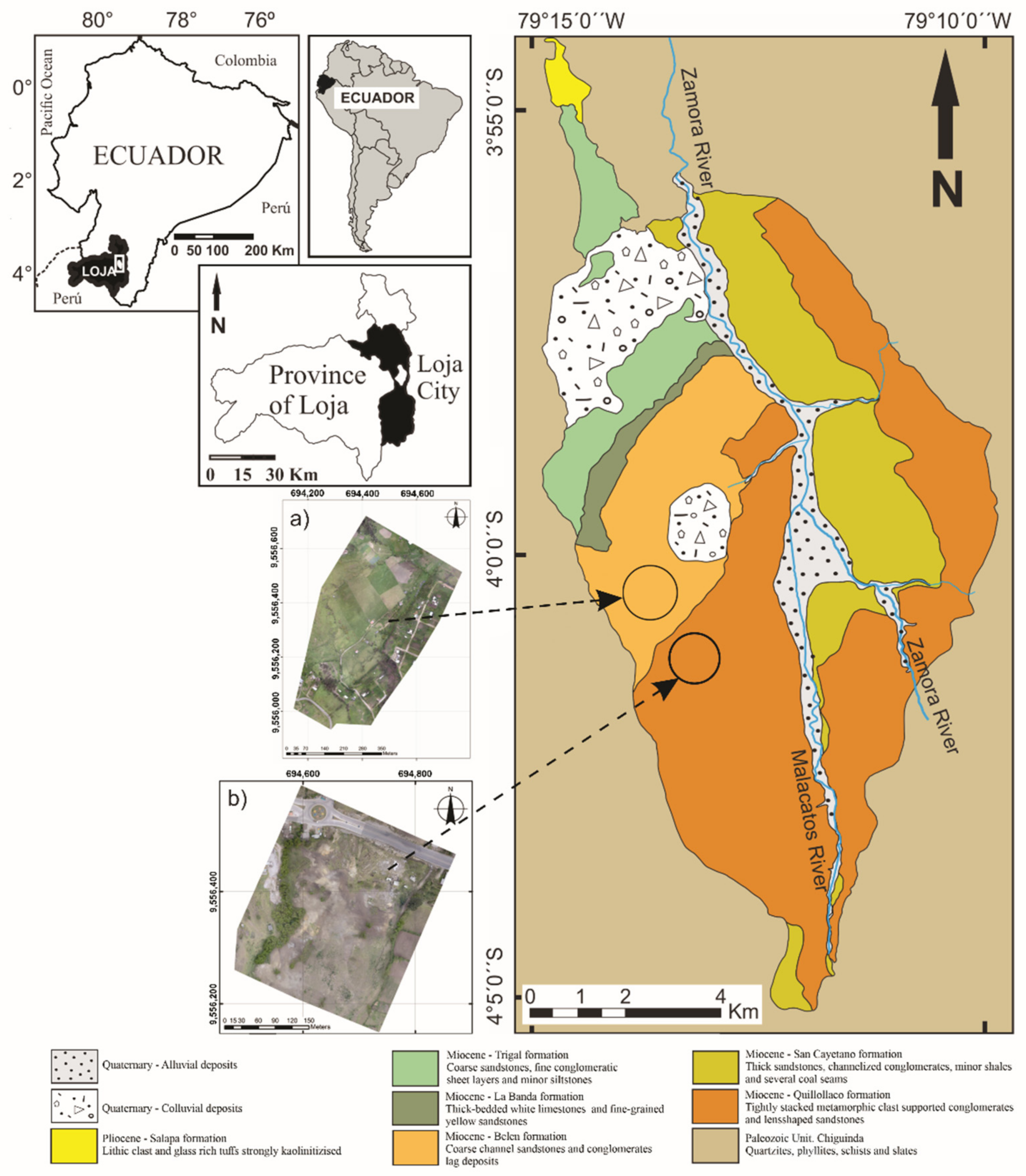
2. Study Areas
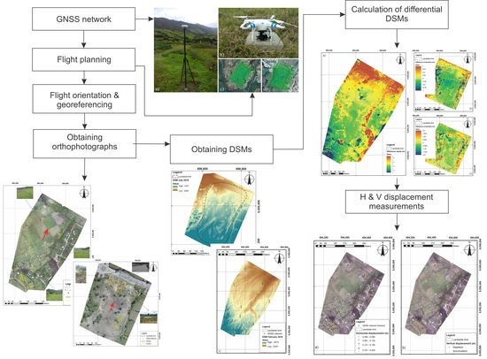
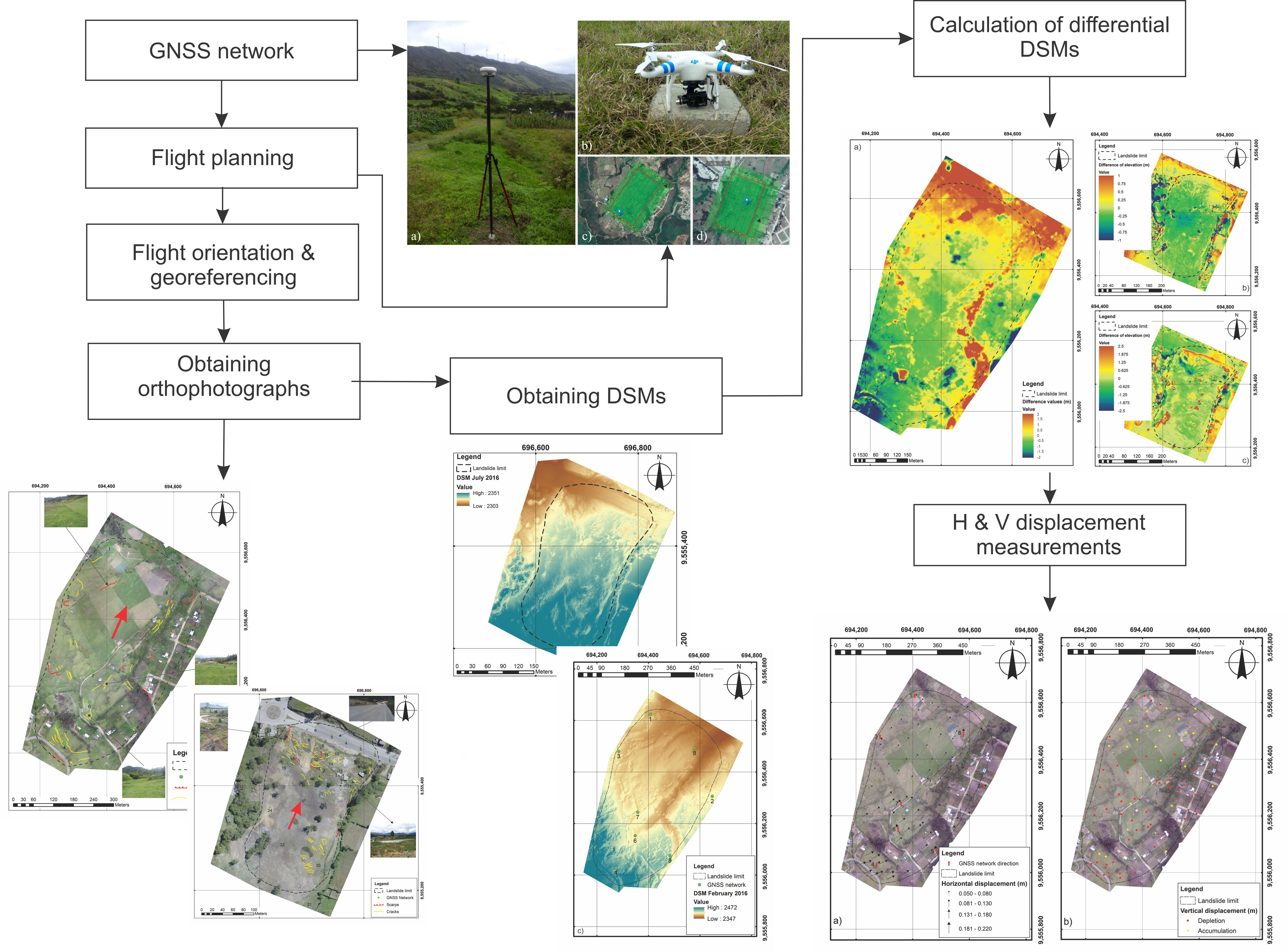
3. Materials and Methods
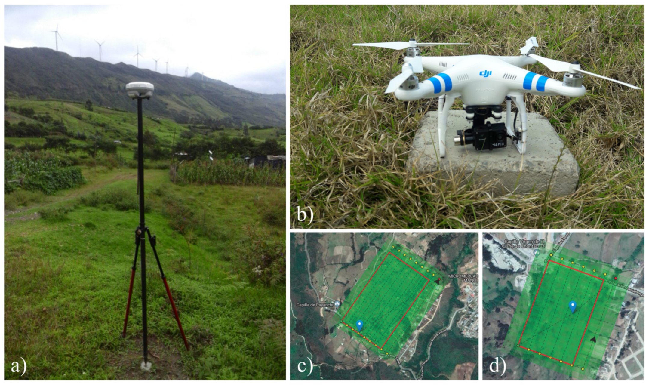
3.1. GNSS Measurements and Processing
3.2. RPAS Values, Orientation, and Data Collection
3.3. Accuracies and Errors
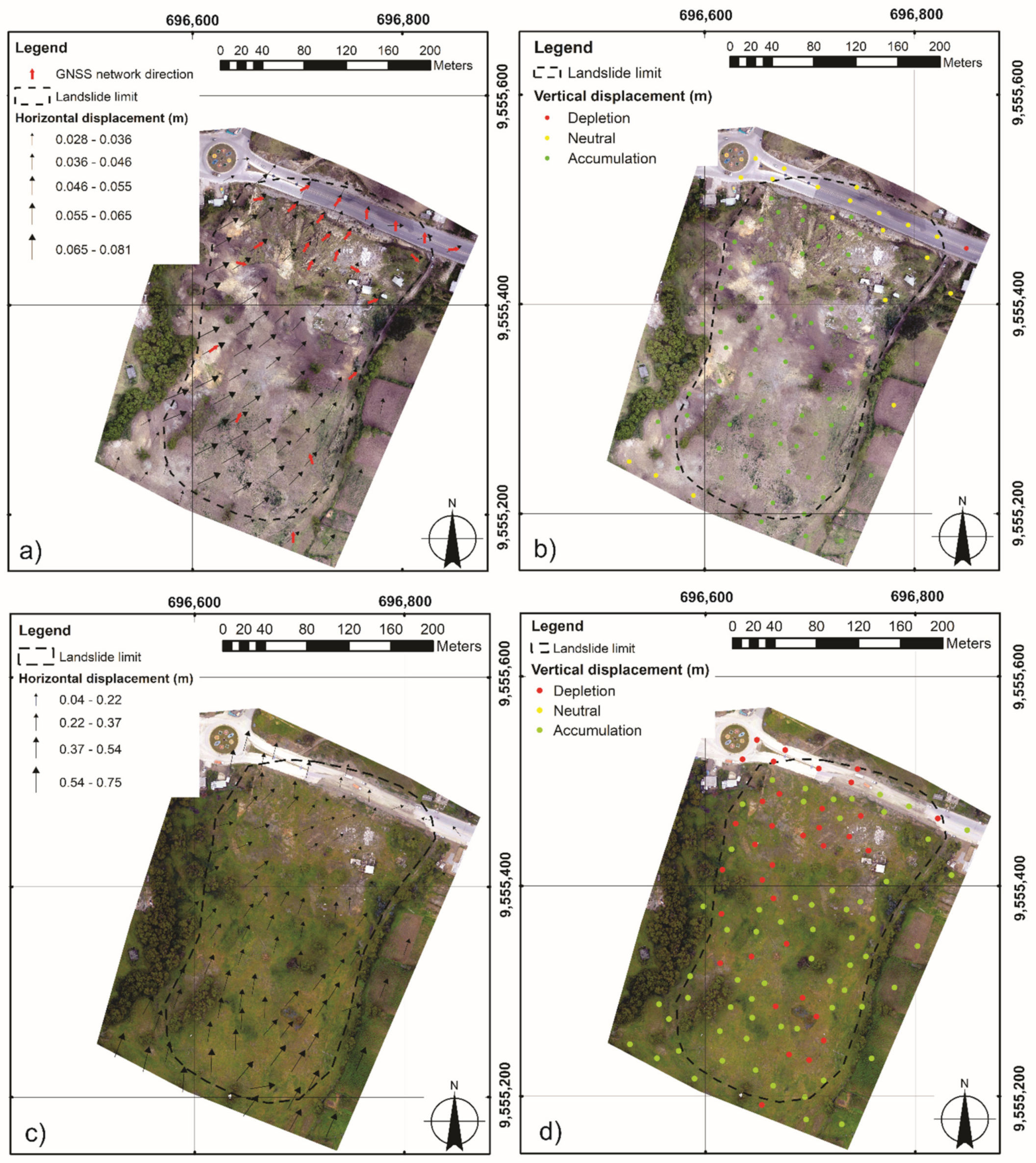
3.4. Displacement Measurements
4. Results
4.1. Displacements in Control Points Measured by GNSS
4.2. Displacements in Monitoring Points Assessed by RPAS
4.3. DSM of Differences (DoDs)
5. Discussion
5.1. Errors and Uncertainties
5.2. Analysis of Displacements in Unstable Zones
5.3. DSM of Differences (DoDs)
6. Conclusions
Author Contributions
Funding
Institutional Review Board Statement
Informed Consent Statement
Data Availability Statement
Acknowledgments
Conflicts of Interest
References
- Agüera-Vega, F.; Carvajal-Ramírez, F.; Martínez-Carricondo, P.; Sánchez-Hermosilla López, J.; Mesas-Carrascosa, F.J.; García-Ferrer, A.; Pérez-Porras, F.J. Reconstruction of extreme topography from UAV structure from motion photogrammetry. Measurement 2018, 121, 127–138. [Google Scholar] [CrossRef]
- Assilzadeh, H.; Levy, J.K.; Wang, X. Landslide catastrophes and disaster risk reduction: A GIS framework for landslide prevention and management. Remote Sens. 2010, 2, 2259–2273. [Google Scholar] [CrossRef] [Green Version]
- Donnini, M.; Napolitano, E.; Salvati, P.; Ardizzone, F.; Bucci, F.; Fiorucci, F.; Santangelo, M.; Cardinali, M.; Guzzetti, F. Impact of event landslides on road networks: A statistical analysis of two Italian case studies. Landslides 2017, 14, 1521–1535. [Google Scholar] [CrossRef]
- Psimoulis, P.A.; Houlié, N.; Habboub, M.; Michel, C.; Rothacher, M. Detection of ground motions using high-rate GPS time-series. Geophys. J. Int. 2018, 214, 1237–1251. [Google Scholar] [CrossRef] [Green Version]
- Choi, K.Y.; Cheung, R.W.M. Landslide disaster prevention and mitigation through works in Hong Kong. J. Rock Mech. Geotech. Eng. 2013, 5, 354–365. [Google Scholar] [CrossRef] [Green Version]
- Fernández, T.; Jiménez, J.; Delgado, J.; Cardenal, J.; Pérez, J.L.; Hamdouni, R.E.; Irigaray, C.; Chacón, J. Methodology for landslide susceptibility and hazard mapping using GIS and SDI. In Intelligent Systems for Crisis Management: Geo-Information for Disaster Management (Gi4DM) 2012; Zlatanova, S., Peters, R., Dilo, A., Scholten, H., Eds.; Springer: Berlin/Heidelberg, Germany, 2013; pp. 185–198. [Google Scholar]
- Kumar, R.; Anbalagan, R. Landslide susceptibility zonation of Tehri reservoir rim region using binary logistic regression model. Curr. Sci. 2015, 108, 1662–1672. [Google Scholar]
- Lari, S.; Frattini, P.; Crosta, G.B. A probabilistic approach for landslide hazard analysis. Eng. Geol. 2014, 182, 3–14. [Google Scholar] [CrossRef] [Green Version]
- Ponomarev, A.A.; Zerkal, O.V.; Samarin, E.N. Protection of the transport infrastructure from influence of landslides by suspension grouting. Procedia Eng. 2017, 189, 880–885. [Google Scholar] [CrossRef]
- Bellone, T.; Dabove, P.; Manzino, A.M.; Taglioretti, C. Real-time monitoring for fast deformations using GNSS low-cost receivers. Geomat. Nat. Hazards Risk 2016, 7, 458–470. [Google Scholar] [CrossRef] [Green Version]
- Capilla, R.M.; Berné, J.L.; Martín, A.; Rodrigo, R. Simulation case study of deformations and landslides using real-time GNSS precise point positioning technique. Geomat. Nat. Hazards Risk 2016, 7, 1856–1873. [Google Scholar] [CrossRef] [Green Version]
- Li, W.; Wang, C. GPS in the tailings dam deformation monitoring. Procedia Eng. 2011, 26, 1648–1657. [Google Scholar] [CrossRef] [Green Version]
- Malet, J.P.; Ferhat, G.; Ulrich, P.; Boetzlé, P. The French national landslide observatory OMIV—Monitoring surface displacement using permanent GNSS, photogrammetric cameras and terrestrial LiDAR for understanding the landslide mechanisms. In Proceedings of the 3rd Joint International Symposium on Deformation Monitoring (JISDM), Vienna, Austria, 30 March–1 April 2016; pp. 1–7. [Google Scholar]
- Hastaoglu, K.O.; Sanli, D.U. Accuracy of GPS rapid static positioning: Application to Koyulhisar landslide, Central Turkey. Surv. Rev. 2011, 43, 226–240. [Google Scholar] [CrossRef]
- Rawat, M.S.M.; Joshi, V.; Rawat, M.S.; Kumar, K. Landslide movement monitoring using GPS technology: A case study of Bakthang landslide, Gangtok, East Sikkim, India. J. Dev. Agric. Econ. 2011, 3, 194–200. [Google Scholar]
- Jaboyedoff, M.; Oppikofer, T.; Abellán, A.; Derron, M.H.; Loye, A.; Metzger, R.; Pedrazzini, A. Use of LIDAR in landslide investigations: A review. Nat. Hazards 2012, 61, 5–28. [Google Scholar] [CrossRef] [Green Version]
- Metternicht, G.; Hurni, L.; Gogu, R. Remote sensing of landslides: An analysis of the potential contribution to geo-spatial systems for hazard assessment in mountainous environments. Remote Sens. Environ. 2005, 98, 284–303. [Google Scholar] [CrossRef]
- Del Soldato, M.; Solari, L.; Poggi, F.; Raspini, F.; Tomás, R.; Fanti, R.; Casagli, N. Landslide-induced damage probability estimation coupling inSAR and field survey data by fragility curves. Remote Sens. 2019, 11, 1486. [Google Scholar] [CrossRef] [Green Version]
- Colesanti, C.; Wasowski, J. Investigating landslides with space-borne Synthetic Aperture Radar (SAR) interferometry. Eng. Geol. 2006, 88, 3–4. [Google Scholar] [CrossRef]
- Miano, A.; Mele, A.; Calcaterra, D.; Di Martire, D.; Infante, D.; Prota, A.; Ramondini, M. The use of satellite data to support the structural health monitoring in areas affected by slow-moving landslides: A potential application to reinforced concrete buildings. Struct. Health Monit. 2021, 1475921720983232. [Google Scholar] [CrossRef]
- Hsieh, Y.C.; Chan, Y.C.; Hu, J.C. Digital elevation model differencing and error estimation from multiple sources: A case study from the Meiyuan Shan landslide in Taiwan. Remote Sens. 2016, 8, 199. [Google Scholar] [CrossRef] [Green Version]
- Medjkane, M.; Maquaire, O.; Costa, S.; Roulland, T.; Letortu, P.; Fauchard, C.; Antoine, R.; Davidson, R. High-resolution monitoring of complex coastal morphology changes: Cross-efficiency of SfM and TLS-based survey (Vaches-Noires cliffs, Normandy, France). Landslides 2018, 15, 1097–1108. [Google Scholar] [CrossRef]
- Cavalli, M.; Marchi, L. Characterisation of the surface morphology of an alpine alluvial fan using airborne LiDAR. Nat. Hazards Earth Syst. Sci. 2008, 8, 323–333. [Google Scholar] [CrossRef]
- Dewitte, O.; Jasselette, J.C.; Cornet, Y.; Van den Eeckhaut, M.; Collignon, A.; Poesen, J.; Demoulin, A. Tracking landslide displacements by multi-temporal DTMs: A combined aerial stereophotogrammetric and LIDAR approach in Western Belgium. Eng. Geol. 2008, 99, 11–22. [Google Scholar] [CrossRef]
- Fernández, T.; Pérez-García, J.L.; Gómez-López, J.M.; Cardenal, J.; Moya, F.; Delgado, J. Multitemporal landslide inventory and activity analysis by means of aerial photogrammetry and LiDAR techniques in an area of Southern Spain. Remote Sens. 2021, 13, 2110. [Google Scholar] [CrossRef]
- Fernández, T.; Pérez, J.; Colomo, C.; Cardenal, J.; Delgado, J.; Palenzuela, J.; Irigaray, C.; Chacón, J. Assessment of the evolution of a landslide using digital photogrammetry and LiDAR techniques in the alpujarras region (Granada, Southeastern Spain). Geosciences 2017, 7, 32. [Google Scholar] [CrossRef] [Green Version]
- Gaprindashvili, G.; Van Westen, C.J. Generation of a national landslide hazard and risk map for the country of Georgia. Nat. Hazards 2016, 80, 69–101. [Google Scholar] [CrossRef]
- Irigaray, C.; Palenzuela, J.A. Análisis de la actividad de movimientos de ladera mediante láser escáner terrestre en el suroeste de la Cordillera Bética (España) landslide activity analysis using terrestrial laser scanning at southwest of the Betic Cordillera (Spain). Rev. Geol. Apl. Ing. Ambiente 2013, 31, 53–67. [Google Scholar]
- Johnson, K.; Nissen, E.; Saripalli, S.; Arrowsmith, R.; McGarey, P.; Scharer, K.; Williams, P.; Blisniuk, K. Rapid mapping of ultrafine fault zone topography with structure from motion. Geosphere 2014, 10, 969–986. [Google Scholar] [CrossRef]
- Kasai, M.; Ikeda, M.; Asahina, T.; Fujisawa, K. LiDAR-derived DEM evaluation of deep-seated landslides in a steep and rocky region of Japan. Geomorphology 2009, 113, 57–69. [Google Scholar] [CrossRef]
- McKean, J.; Roering, J. Objective landslide detection and surface morphology mapping using high-resolution airborne laser altimetry. Geomorphology 2004, 57, 331–351. [Google Scholar] [CrossRef]
- Růžičková, K.; Inspektor, T. Surface Models for Geosciences. Lecture Notes in Geoinformation and Cartography; Springer: Cham, Switzerland, 2015. [Google Scholar]
- Tiwari, A.; Narayan, A.B.; Devara, M.; Dwivedi, R.; Dikshit, O. Multi-sensor geodetic approach for landslide detection and monitoring. In Proceedings of the ISPRS Annals of the Photogrammetry, Remote Sensing and Spatial Information Sciences, Dehradun, India, 20–23 November 2018. [Google Scholar]
- ASPRS. ASPRS accuracy standards for large-scale maps. Photogramm. Eng. Remote Sens. 1990, 56, 1068–1070. [Google Scholar]
- Boccardo, P.; Chiabrando, F.; Dutto, F.; Tonolo, F.G.; Lingua, A. UAV deployment exercise for mapping purposes: Evaluation of emergency response applications. Sensors 2015, 15, 15717–15737. [Google Scholar] [CrossRef] [Green Version]
- Chen, B.; Yang, Y.; Wen, H.; Ruan, H.; Zhou, Z.; Luo, K.; Zhong, F. High-resolution monitoring of beach topography and its change using unmanned aerial vehicle imagery. Ocean. Coast. Manag. 2018, 160, 103–116. [Google Scholar] [CrossRef]
- Kasperski, J.; Delacourt, C.; Allemand, P.; Potherat, P.; Jaud, M.; Varrel, E. Application of a terrestrial laser scanner (TLS) to the study of the séchilienne landslide (Isère, France). Remote Sens. 2010, 2, 2785–2802. [Google Scholar] [CrossRef] [Green Version]
- Mozas-Calvache, A.T.; Pérez-García, J.L.; Fernández, T. Monitoring of landslide displacements using UAS and control methods based on lines. Landslides 2017, 14, 2115–2128. [Google Scholar] [CrossRef]
- Prokešová, R.; Kardoš, M.; Medvedová, A. Landslide dynamics from high-resolution aerial photographs: A case study from the Western Carpathians, Slovakia. Geomorphology 2010, 115, 90–101. [Google Scholar] [CrossRef]
- Walstra, J.; Chandler, J.H.; Dixon, N.; Dijkstra, T. Time for change-quantifying landslide evolution using historical aerial photographs and modern photogrammetric methods. In Proceedings of the ISPRS International Archives of the Photogrammetry, Remote Sensing and Spatial Information Sciences, Dresden, Germany, 12–22 February 2004; pp. 475–480. [Google Scholar]
- Stumpf, A.; Malet, J.P.; Allemand, P.; Pierrot-Deseilligny, M.; Skupinski, G. Ground-based multi-view photogrammetry for the monitoring of landslide deformation and erosion. Geomorphology 2015, 231, 130–145. [Google Scholar] [CrossRef]
- Eltner, A.; Kaiser, A.; Castillo, C.; Rock, G.; Neugirg, F.; Abellán, A. Image-based surface reconstruction in geomorphometry—Merits, limits and developments. Earth Surf. Dynam. 2016, 4, 359–389. [Google Scholar] [CrossRef] [Green Version]
- Seitz, S.M.; Curless, B.; Diebel, J.; Scharstein, D.; Szeliski, R. A comparison and evaluation of multi-view stereo reconstruction algorithms. In Proceedings of the IEEE Computer Society Conference on Computer Vision and Pattern Recognition (CVPR’06), New York, NY, USA, 17–22 June 2006; pp. 519–528. [Google Scholar]
- Agisoft. Agisoft Photoscan User Manual: Professional Edition (Version 1.4); Agisoft LLC: Petersburg, Russia, 2018. [Google Scholar]
- González-Aguilera, D.; López-Fernández, L.; Rodriguez-Gonzalvez, P.; Guerrero, D.; Hernandez-Lopez, D.; Remondino, F.; Menna, F.; Nocerino, E.; Toschi, I.B.A.; Gaiani, M. Development of an all-purpose free photogrammetric tool. In Proceedings of the ISPRS International Archives of the Photogrammetry, Remote Sensing and Spatial Information Sciences, Prague, Czech Republic, 12–19 July 2016; pp. 31–38. [Google Scholar]
- Pix4D Mapper. Available online: https://www.pix4d.com/product/pix4dmapper-photogrammetry-software (accessed on 11 March 2021).
- Al-Rawabdeh, A.; Al-Gurrani, H.; Al-Durgham, K.; Detchev, I.; He, F.; El-Sheimy, N.; Habib, A. A robust registration algorithm for point clouds from UAV images for change detection. Int. Arch. Photogramm. Remote Sens. Spat. Inf. Sci. 2016, 41, 765–772. [Google Scholar] [CrossRef] [Green Version]
- Fernández, T.; Pérez, J.L.; Cardenal, F.J.; López, A.; Gómez, J.M.; Colomo, C.; Delgado, J.; Sánchez, M. Use of a light UAV and photogrammetric techniques to study the evolution of a landslide in Jaén (Southern Spain). In Proceedings of the International Archives of the Photogrammetry, Remote Sensing and Spatial Information Sciences, La Grande Motte, France, 28 September–3 October 2015; pp. 241–248. [Google Scholar]
- Niethammer, U.; Rothmund, S.; Schwaderer, U.; Zeman, J.; Joswig, M. Open source image-processing tools for low-cost UAV-based landslide investigations. In Proceedings of the ISPRS International Archives of the Photogrammetry, Remote Sensing and Spatial Information Sciences, Zurich, Switzerland, 14–16 September 2011; pp. 161–166. [Google Scholar]
- Peppa, M.V.; Mills, J.P.; Moore, P.; Miller, P.E.; Chambers, J.E. Accuracy assessment of a UAV-based landslide monitoring system. In Proceedings of the ISPRS International Archives of the Photogrammetry, Remote Sensing and Spatial Information Sciences, Prague, Czech Republic, 12–19 July 2016. [Google Scholar]
- Stumpf, A.; Malet, J.P.; Kerle, N.; Niethammer, U.; Rothmund, S. Image-based mapping of surface fissures for the investigation of landslide dynamics. Geomorphology 2013, 186, 12–27. [Google Scholar] [CrossRef] [Green Version]
- Lindner, G.; Schraml, K.; Mansberger, R.; Hübl, J. UAV monitoring and documentation of a large landslide. Appl. Geomat. 2016, 8, 1–11. [Google Scholar] [CrossRef]
- Mozas-Calvache, A.T.; Pérez-García, J.L.; Fernández, T.; Gómez-López, J.M.; Colomo-Jiménez, C. Analysis of landslides based on displacements of lines. In Proceedings of the ISPRS International Archives of the Photogrammetry, Remote Sensing and Spatial Information Sciences, Prague, Czech Republic, 12–19 July 2016. [Google Scholar]
- Peppa, M.V.; Mills, J.P.; Moore, P.; Miller, P.E.; Chambers, J.E. Automated co-registration and calibration in SfM photogrammetry for landslide change detection. Earth Surf. Process. Landf. 2019, 44, 287–303. [Google Scholar] [CrossRef] [Green Version]
- Peternel, T.; Kumelj, Š.; Oštir, K.; Komac, M. Monitoring the Potoška planina landslide (NW Slovenia) using UAV photogrammetry and tachymetric measurements. Landslides 2017, 14, 395–406. [Google Scholar] [CrossRef]
- Rossi, G.; Tanteri, L.; Tofani, V.; Vannocci, P.; Moretti, S.; Casagli, N. Multitemporal UAV surveys for landslide mapping and characterization. Landslides 2018, 15, 1045–1052. [Google Scholar] [CrossRef] [Green Version]
- Turner, D.; Lucieer, A.; De Jong, S.M. Time series analysis of landslide dynamics using an Unmanned Aerial Vehicle (UAV). Remote Sens. 2015, 7, 1736–1757. [Google Scholar] [CrossRef] [Green Version]
- Warrick, J.A.; Ritchie, A.C.; Schmidt, K.M.; Reid, M.E.; Logan, J. Characterizing the catastrophic 2017 Mud Creek landslide, California, using repeat structure-from-motion (SfM) photogrammetry. Landslides 2019, 16, 1201–1219. [Google Scholar] [CrossRef]
- Fernández, T.; Pérez, J.L.; Cardenal, J.; Gómez, J.M.; Colomo, C.; Delgado, J. Analysis of landslide evolution affecting olive groves using UAV and photogrammetric techniques. Remote Sens. 2016, 8, 837. [Google Scholar] [CrossRef] [Green Version]
- Soto, J.; Galve, J.P.; Palenzuela, J.A.; Azañón, J.M.; Tamay, J.; Irigaray, C. A multi-method approach for the characterization of landslides in an intramontane basin in the Andes (Loja, Ecuador). Landslides 2017, 14, 1929–1947. [Google Scholar] [CrossRef]
- Hungerbühler, D.; Steinmann, M.; Winkler, W.; Seward, D.; Egüez, A.; Peterson, D.E.; Helg, U.; Hammer, C. Neogene stratigraphy and Andean geodynamics of Southern Ecuador. Earth Sci. Rev. 2002, 57, 75–124. [Google Scholar] [CrossRef]
- Wang, G. Millimeter-accuracy GPS landslide monitoring using Precise Point Positioning with Single Receiver Phase Ambiguity (PPP-SRPA) resolution: A case study in Puerto Rico. J. Geod. Soc. 2013, 3, 22–31. [Google Scholar] [CrossRef]
- Akbarimehr, M.; Motagh, M.; Haghshenas-Haghighi, M. Slope stability assessment of the sarcheshmeh landslide, Northeast Iran, investigated using InSAR and GPS observations. Remote Sens. 2013, 5, 3681–3700. [Google Scholar] [CrossRef] [Green Version]
- Pesci, A.; Teza, G.; Casula, G.; Fabris, M.; Bonforte, A. Remote sensing and geodetic measurements for volcanic slope monitoring: Surface variations measured at Northern Flank of La Fossa Cone (Vulcano Island, Italy). Remote Sens. 2013, 5, 2238–2256. [Google Scholar] [CrossRef] [Green Version]
- Gili, J.; Jordi, C.; Joan, R. Using Global Positioning System techniques in landslide monitoring. Eng. Geol. 2000, 55, 167–192. [Google Scholar] [CrossRef]
- Zárate, B. Monitoreo de movimientos de ladera en el sector de San Pedro de Vilcabamba mediante procedimientos GPS. Maskana 2011, 2, 17–25. [Google Scholar] [CrossRef]
- Car, M.; Kaćunić, D.J.; Kovačević, M.S. Application of unmanned aerial vehicle for landslide mapping. In Proceedings of the International Symposium on Engineering Geodesy, Varazdin, Croatia, 20–22 May 2016; pp. 549–560. [Google Scholar]
- Hackney, C.; Clayton, A. Unmanned aerial vehicles (UAVs) and their application in geomorphic mapping. Geomorphol. Tech. 2015, 7, 1–12. [Google Scholar]
- Mozas-Calvache, A.T.; Pérez-García, J.L.; Cardenal-Escarcena, F.J.; Mata-Castro, E.; Delgado-García, J. Method for photogrammetric surveying of archaeological sites with light aerial platforms. J. Archaeol. Sci. 2012, 39, 521–530. [Google Scholar] [CrossRef]
- Uysal, M.; Toprak, A.S.; Polat, N. DEM generation with UAV photogrammetry and accuracy analysis in Sahitler hill. Measurement 2015, 73, 539–543. [Google Scholar] [CrossRef]
- Yucel, M.A.; Turan, R.Y. Areal change detection and 3D modeling of mine lakes using high-resolution Unmanned Aerial Vehicle images. Arab. J. Sci. Eng. 2016, 41, 4867–4878. [Google Scholar] [CrossRef]
- Bossi, G.; Cavalli, M.; Crema, S.; Frigerio, S.; Quan Luna, B.; Mantovani, M.; Marcato, G.; Schenato, L.; Pasuto, A. Multi-temporal LiDAR-DTMs as a tool for modelling a complex landslide: A case study in the Rotolon catchment (Eastern Italian Alps). Nat. Hazards Earth Syst. Sci. 2015, 15, 715–722. [Google Scholar] [CrossRef] [Green Version]
- Wheaton, J.M.; Brasington, J.; Darby, S.E.; Sear, D.A. Accounting for uncertainty in DEMs from repeat topographic surveys: Improved sediment budgets. Earth Surf. Process. Landf. 2010, 35, 136–156. [Google Scholar] [CrossRef]
- Agüera-Vega, F.; Carvajal-Ramírez, F.; Martínez-Carricondo, P. Accuracy of digital surface models and orthophotos derived from Unmanned Aerial Vehicle photogrammetry. J. Surv. Eng. 2016, 143, 04016025. [Google Scholar] [CrossRef]
- Carvajal, F.; Agüera, F.; Pérez, M. Surveying a landslide in a road embankment using unmanned aerial vehicle photogrammetry. In Proceedings of the ISPRS International Archives of the Photogrammetry, Remote Sensing and Spatial Information Sciences XXXVIII-1/C22, Zurich, Switzerland, 14–16 September 2011; pp. 201–206. [Google Scholar]
- Kršák, B.; Blišťan, P.; Pauliková, A.; Puškárová, P.; Kovanič, Ľ.; Palková, J.; Zelizňaková, V. Use of low-cost UAV photogrammetry to analyze the accuracy of a digital elevation model in a case study. Measurement 2016, 91, 276–287. [Google Scholar] [CrossRef]
- Vrublová, D.; Roman, K.; Jiránková, E.; Adam, S. Documentation of landslides and inaccessible parts of a mine using an unmanned UAV system and methods of digital terrestrial photogrammetry. GeoSci. Eng. 2015, 61, 8–19. [Google Scholar] [CrossRef] [Green Version]
- Cruden, D.; Varnes, D.J. Landslide types and processes. In Landslides: Investigation and Mitigation; Turner, A.K., Schuster, R.L., Eds.; National Academy Press: Washington, DC, USA, 1996; pp. 36–75. [Google Scholar]
- Hungr, O.; Leroueil, S.; Picarelli, L. The varnes classification of landslide types, an update. Landslides 2014, 11, 167–194. [Google Scholar] [CrossRef]
- WP/WLI. Describing Landslides in Several Languages: The Multilingual Landslide Glossary; Bitech Publishers: Richmond, BC, Canada, 1993. [Google Scholar]
- Cardenal, J.; Fernández, T.; Pérez-García, J.L.; Gómez-López, J.M. Measurement of road surface deformation using images captured from UAVs. Remote Sens. 2009, 11, 1507. [Google Scholar] [CrossRef] [Green Version]


| Study Area | Campaign | Measurement Date | Cumulative Time Span (Days) |
|---|---|---|---|
| Victoria | 1 | 18 January 2016 | 1 |
| 2 | 18 February 2016 | 32 | |
| 3 | 10 March 2016 | 53 | |
| 4 | 23 March 2016 | 66 | |
| 5 | 21 May 2016 | 125 | |
| 6 | 11 June 2016 | 146 | |
| Colinas Lojanas | 1 | 22 August 2016 | 1 |
| 2 | 6 September 2016 | 16 | |
| 3 | 29 September 2016 | 36 | |
| 4 | 13 October 2016 | 53 | |
| 5 | 28 October 2016 | 68 | |
| 6 | 23 November 2016 | 94 |
| Area | Victoria | Colinas Lojanas | |||
|---|---|---|---|---|---|
| Date | 18 February 2016 | 11 June 2016 | 4 July 2016 | 29 November 2016 | 12 January 2018 |
| No. of images acquired | 243 | 268 | 216 | 221 | 208 |
| No. of images used | 226 | 246 | 188 | 190 | 186 |
| Forward overlap | 70% | 70% | 70% | 70% | 70% |
| Side overlap | 60% | 60% | 60% | 60% | 60% |
| Flight height | 120 m | 119 m | 97.4 m | 77.3 m | 92.2 m |
| Number of flyovers | 14 | 14 | 12 | 12 | 12 |
| North alignment | 35° | 35° | 20° | 20° | 20° |
| Photographic resolution (px) | 1.74 × 1.74 | 1.74 × 1.74 | 1.74 × 1.74 | 1.74 × 1.74 | 1.74 × 1.74 |
| Processing Results | Victoria | Colinas Lojanas | |||
|---|---|---|---|---|---|
| 18 February 2016 | 11 June 2016 | 4 July 2016 | 29 November 2016 | 12 January 2018 | |
| Number of processed images | 226 | 246 | 289 | 285 | 278 |
| Number of GCPs | 5 | 5 | 6 | 6 | 6 |
| XY error (m) | 0.025 | 0.053 | 0.056 | 0.038 | 0.028 |
| Z error (m) | 0.038 | 0.024 | 0.040 | 0.059 | 0.103 |
| Total RMSE (cm) | 0.045 | 0.053 | 0.069 | 0.070 | 0.030 |
| Number of checkpoints | 3 | 3 | 4 | 4 | 4 |
| XY error (cm) | 0.026 | 0.056 | 0.039 | 0.026 | 0.026 |
| Z error (cm) | 0.041 | 0.042 | 0.061 | 0.041 | 0.039 |
| Total RMSE (cm) | 0.049 | 0.070 | 0.073 | 0.049 | 0.047 |
| Ground simple distance (GSD) (m px−1) | 0.060 | 0.060 | 0.070 | 0.070 | 0.070 |
| GNSS Point | N (m) | E (m) | Z (m) | DNE (m) | VH (m month−1) | VV (m month−1) | Direction |
|---|---|---|---|---|---|---|---|
| 1 | −0.029 | 0.048 | −0.025 | 0.056 | 0.017 | −0.008 | E |
| 2 | −0.028 | 0.104 | −0.031 | 0.108 | 0.035 | −0.010 | E |
| 3 | −0.057 | 0.080 | −0.040 | 0.098 | 0.031 | −0.013 | S 54.5°E |
| 4 | 0.118 | 0.114 | −0.037 | 0.164 | 0.052 | −0.012 | N 44.0°E |
| 5 | 0.212 | −0.043 | −0.098 | 0.216 | 0.069 | −0.031 | N 11.5°W |
| 6 | 0.178 | −0.088 | −0.076 | 0.199 | 0.064 | −0.024 | N 26.3°W |
| 7 | 0.154 | −0.036 | −0.068 | 0.158 | 0.050 | −0.022 | N |
| 8 | 0.181 | −0.015 | −0.055 | 0.181 | 0.058 | −0.018 | N |
| GNSS Point | N (m) | E (m) | Z (m) | DNE (m) | VH (m month−1) | VV (m month−1) | Direction |
|---|---|---|---|---|---|---|---|
| 1 | −0.015 | 0.029 | 0.038 | 0.033 | 0.010 | 0.011 | - |
| 2 | 0.034 | 0.017 | 0.069 | 0.038 | 0.011 | 0.020 | N |
| 3 | 0.017 | 0.012 | 0.093 | 0.021 | 0.006 | 0.027 | - |
| 4 | 0.036 | 0.016 | 0.104 | 0.039 | 0.011 | 0.030 | NNE |
| 5 | 0.002 | 0.026 | 0.061 | 0.026 | 0.007 | 0.018 | E |
| 6 | 0.035 | 0.018 | 0.036 | 0.039 | 0.011 | 0.010 | NNE |
| 7 | 0.052 | 0.010 | −0.042 | 0.053 | 0.015 | −0.012 | N |
| 8 | 0.084 | 0.070 | −0.060 | 0.109 | 0.031 | −0.017 | NE |
| 9 | 0.089 | 0.072 | 0.047 | 0.114 | 0.033 | 0.014 | N 38.9 E |
| 10 | 0.097 | 0.078 | −0.126 | 0.124 | 0.036 | −0.036 | N 38.8 E |
| 11 | 0.039 | 0.048 | −0.070 | 0.062 | 0.018 | −0.020 | N 50.9 E |
| 12 | 0.026 | 0.049 | −0.057 | 0.055 | 0.016 | −0.016 | ENE |
| 13 | 0.036 | 0.078 | −0.170 | 0.086 | 0.025 | −0.049 | N 65.2 E |
| 14 | 0.018 | 0.065 | −0.051 | 0.067 | 0.019 | −0.015 | ENE |
| 15 | −0.027 | 0.044 | −0.053 | 0.052 | 0.015 | −0.015 | SE |
| 16 | −0.036 | 0.036 | −0.095 | 0.051 | 0.015 | −0.027 | S 45.0 E |
| 17 | 0.143 | 0.050 | −0.108 | 0.151 | 0.044 | −0.031 | NNE 19.3 E |
| 18 | 0.040 | 0.024 | 0.062 | 0.047 | 0.014 | −0.018 | NNE |
| 19 | −0.028 | 0.114 | −0.184 | 0.117 | 0.034 | −0.053 | ESE |
| 20 | 0.142 | −0.040 | −0.111 | 0.148 | 0.043 | −0.032 | N 15.7 W |
| 21 | 0.024 | 0.023 | −0.111 | 0.033 | 0.010 | −0.032 | - |
| 22 | 0.021 | 0.043 | −0.100 | 0.048 | 0.014 | −0.029 | ESE |
| 23 | 0.036 | 0.031 | −0.051 | 0.048 | 0.014 | −0.015 | NE |
| 24 | 0.048 | 0.034 | −0.042 | 0.059 | 0.017 | −0.012 | NNE |
| Error XY | Reference Flight | ||
| 18 February 2016 | |||
| Comparison flight | M | SD | RMSE |
| 11 June 2016 | 0.016 | 0.098 | 0.089 |
| Error Z | Reference Flight | ||
| 18 February 2016 | |||
| Comparison flight | M | SD | RMSE |
| 11 June 2016 | 0.010 | 0.074 | 0.068 |
| Reference Flight | 4 July 2016 | 29 November 2016 | |||||
|---|---|---|---|---|---|---|---|
| Comparison Flight | M | SD | RMSE | M | SD | RMSE | |
| Error XY (m) | 29 November 2016 | 0.032 | 0.015 | 0.035 | - | - | - |
| 12 January 2018 | 0.029 | 0.018 | 0.032 | 0.047 | 0.073 | 0.081 | |
| Error Z (m) | 29 November 2016 | −0.025 | 0.059 | 0.061 | - | - | - |
| 12 January 2018 | −0.027 | 0.049 | 0.058 | −0.019 | 0.066 | 0.065 | |
| Period | Total | Head | Main body | Foot | |||||
|---|---|---|---|---|---|---|---|---|---|
| Absolute (m) | Velocity (m month−1) | Absolute (m) | Velocity (m month−1) | Absolute (m) | Velocity (m month−1) | Absolute (m) | Velocity (m month−1) | ||
| Horizontal displacement (m) | 18 February 2016–11 June 2016 | 0.103 | 0.026 | 0.145 | 0.038 | 0.081 | 0.021 | 0.081 | 0.021 |
| Displacement vertical (m) | 18 February 2016–11 June 2016 | −0.079 | −0.021 | −0.092 | −0.024 | −0.085 | −0.022 | 0.211 | 0.055 |
| Period | Total | Head | Main body | Foot | |||||
|---|---|---|---|---|---|---|---|---|---|
| Absolute (m) | Velocity (m month−1) | Absolute (m) | Velocity (m month−1) | Absolute (m) | Velocity (m month−1) | Absolute (m) | Velocity (m month−1) | ||
| Displacement horizontal | 4 July 2016–29 November 2016 | 0.052 | 0.010 | 0.056 | 0.011 | 0.054 | 0.011 | 0.045 | 0.001 |
| 29 November 2016–12 January 2018 | 0.356 | 0.025 | 0.531 | 0.038 | 0.316 | 0.022 | 0.221 | 0.016 | |
| Displacement vertical | 4 July 2016–29 November 2016 | 0.184 | 0.037 | −0.165 | −0.033 | −0.325 | −0.065 | 0.063 | 0.013 |
| 29 November 2016–12 January 2018 | 0.194 | 0.014 | −0.342 | −0.024 | −0.187 | −0.013 | 0.054 | 0.004 | |
Publisher’s Note: MDPI stays neutral with regard to jurisdictional claims in published maps and institutional affiliations. |
© 2021 by the authors. Licensee MDPI, Basel, Switzerland. This article is an open access article distributed under the terms and conditions of the Creative Commons Attribution (CC BY) license (https://creativecommons.org/licenses/by/4.0/).
Share and Cite
Zárate, B.A.; El Hamdouni, R.; Fernández, T. GNSS and RPAS Integration Techniques for Studying Landslide Dynamics: Application to the Areas of Victoria and Colinas Lojanas, (Loja, Ecuador). Remote Sens. 2021, 13, 3496. https://doi.org/10.3390/rs13173496
Zárate BA, El Hamdouni R, Fernández T. GNSS and RPAS Integration Techniques for Studying Landslide Dynamics: Application to the Areas of Victoria and Colinas Lojanas, (Loja, Ecuador). Remote Sensing. 2021; 13(17):3496. https://doi.org/10.3390/rs13173496
Chicago/Turabian StyleZárate, Belizario A., Rachid El Hamdouni, and Tomás Fernández. 2021. "GNSS and RPAS Integration Techniques for Studying Landslide Dynamics: Application to the Areas of Victoria and Colinas Lojanas, (Loja, Ecuador)" Remote Sensing 13, no. 17: 3496. https://doi.org/10.3390/rs13173496
APA StyleZárate, B. A., El Hamdouni, R., & Fernández, T. (2021). GNSS and RPAS Integration Techniques for Studying Landslide Dynamics: Application to the Areas of Victoria and Colinas Lojanas, (Loja, Ecuador). Remote Sensing, 13(17), 3496. https://doi.org/10.3390/rs13173496