On-Board Volcanic Eruption Detection through CNNs and Satellite Multispectral Imagery

Abstract

In recent years, the growth of Machine Learning (ML) algorithms has raised the number of studies including their applicability in a variety of different scenarios. Among all, one of the hardest ones is the aerospace, due to its peculiar physical requirements. In this context, a feasibility study, with a prototype of an on board Artificial Intelligence (AI) model, and realistic testing equipment and scenario are presented in this work. As a case study, the detection of volcanic eruptions has been investigated with the objective to swiftly produce alerts and allow immediate interventions. Two Convolutional Neural Networks (CNNs) have been designed and realized from scratch, showing how to efficiently implement them for identifying the eruptions and at the same time adapting their complexity in order to fit on board requirements. The CNNs are then tested with experimental hardware, by means of a drone with a paylod composed of a generic processing unit (Raspberry PI), an AI processing unit (Movidius stick) and a camera. The hardware employed to build the prototype is low-cost, easy to found and to use. Moreover, the dataset has been published on GitHub, made available to everyone. The results are promising and encouraging toward the employment of the proposed system in future missions, given that ESA has already moved the first steps of AI on board with the Phisat-1 satellite, launched on September 2020.

1. Introduction

Nowadays, Remote Sensing (RS) is seeing its maximum expanse in terms of applicability and use cases, because of the extremely large availability of remote-sensed images, mostly satellite-based, allowing many scientists from different research fields to approach RS applications [1,2,3]. Among all the possible fields of RS, this manuscript focuses on the object/event detection in satellite imagery with the final goal to implement related AI-based algorithms on board the satellites.

In recent years, the peculiar field of object/event detection in RS has been largely explored with several works employing Synthetic Aperture Radar (SAR) data, for instance for ship detection [4,5,6,7,8,9], and other works using optical data for landslide detection [10,11] or cloud detection [12], just to cite a few. A notable example is the increasing use of this type of data in Earth science and geological fields for monitoring parameters which by their nature are or may become difficult to measure, or that need a lot of time and efforts to be recorded with classical instruments [13].

Although most of the data processing is usually carried out on ground, there have been in the last years some attempts on bringing the computation effort, or at least a part of it, on board the satellites [14]. The ultimate frontier of satellite RS is right represented by the implementation of AI algorithms on board the satellites for scene classification, cloud masking, and hazard detection, which has seen the European Space Agency (ESA) as a pioneer in moving the first steps with the Phisat-1 satellite, launched on September the 3rd 2020 [15,16]. With this mission, it has been shown how AI models can help recognizing too cloudy images thus avoiding to download them toward the Ground Stations and therefore reducing the data transmission load [12]. Another example of AI on board system has been presented in [17], where authors proposed an on board real-time ship detector using SAR data and based on Deep Learning.

Unlike the previous work, the aim of our study has been to investigate the possibility of using optical/multispectral satellite images to monitor hazardous events, specifically volcanic eruption, by means of AI techniques and on board computing resources [18]. The results achieved for the classification of volcanic eruptions could be suitable for future satellite missions such as the next ones from the ESA Phisat program.

It is worth to highlight that, to the best of the authors’ knowledge, there are no similar algorithms in the literature for volcanic eruption detection, also making use of free optical/multispectral images. Indeed, many researchers have made use of satellite images, and SAR data in particular, to monitor ground movements in proximity of a volcano’s crater just before the eruption, which appears interesting but it is something completely different from our approach. An example of AI techniques used to recognize volcano-seismic events is given in [19], where the authors are using two Deep Neural Networks and volcano-seismic data, together with a combined feature vector of linear prediction coefficients and statistical properties, for the classification of seismic events. Other similar approaches can be found in [20,21,22], where respectively real and simulated Interferometric SAR (InSAR) data have been used for detecting volcano surface deformation. Another very interesting work shows how AI plays a key role in monitoring a variety of volcanic processes when multiple sensors are exploited (Sentinel-1 SAR, Sentinel-2 Short-Wave InfraRed (SWIR), Sentinel-5P TROPOMI, with and without the presence of $S{O}_2$ gas emission) [23].

In our manuscript, we propose two different CNNs for the detection of volcanic eruptions by using satellite optical/multispectral images, and the main objective is the leveraging of an on board CNN, that is not considered in the current state-of-the-art.

It is worth to underline that the chosen use case, the volcanic eruption detection, should be considered independent from the on board analysis. Indeed, a similar study for AI on board may be conducted on a different use case. Moreover it is noteworthy to highlight that volcanic ejecta including Sulfur oxides can be detected with SWIR radiometer and so among possible future developments there can be also the exploration of SWIR radiometer data at this end [23,24,25,26].

In our work Sentinel-2 and Landsat-7 optical data have been considered, and the main contributions are the following:

• The on board detection of volcanic eruptions by CNN approaches has never been taken into consideration so far, to the best of the authors’ knowledge.
• The proposed CNN is discussed with regard to the constraints imposed by the on board implementation, which means that the starting network has been optimized and modified in order to be consistent with the target hardware architectures.
• The performances of the CNN deployed on the target hardware are analyzed and discussed after the execution of experimental tests.

The paper is organized as follows: Section 2 deals with the description of the volcanic eruptions dataset, while Section 3 presents the CNN models explored in this study. In Section 4 the on board implementation of the proposed detection approach is analyzed. Results and discussion are presented in Section 5. Conclusions are given at the end.

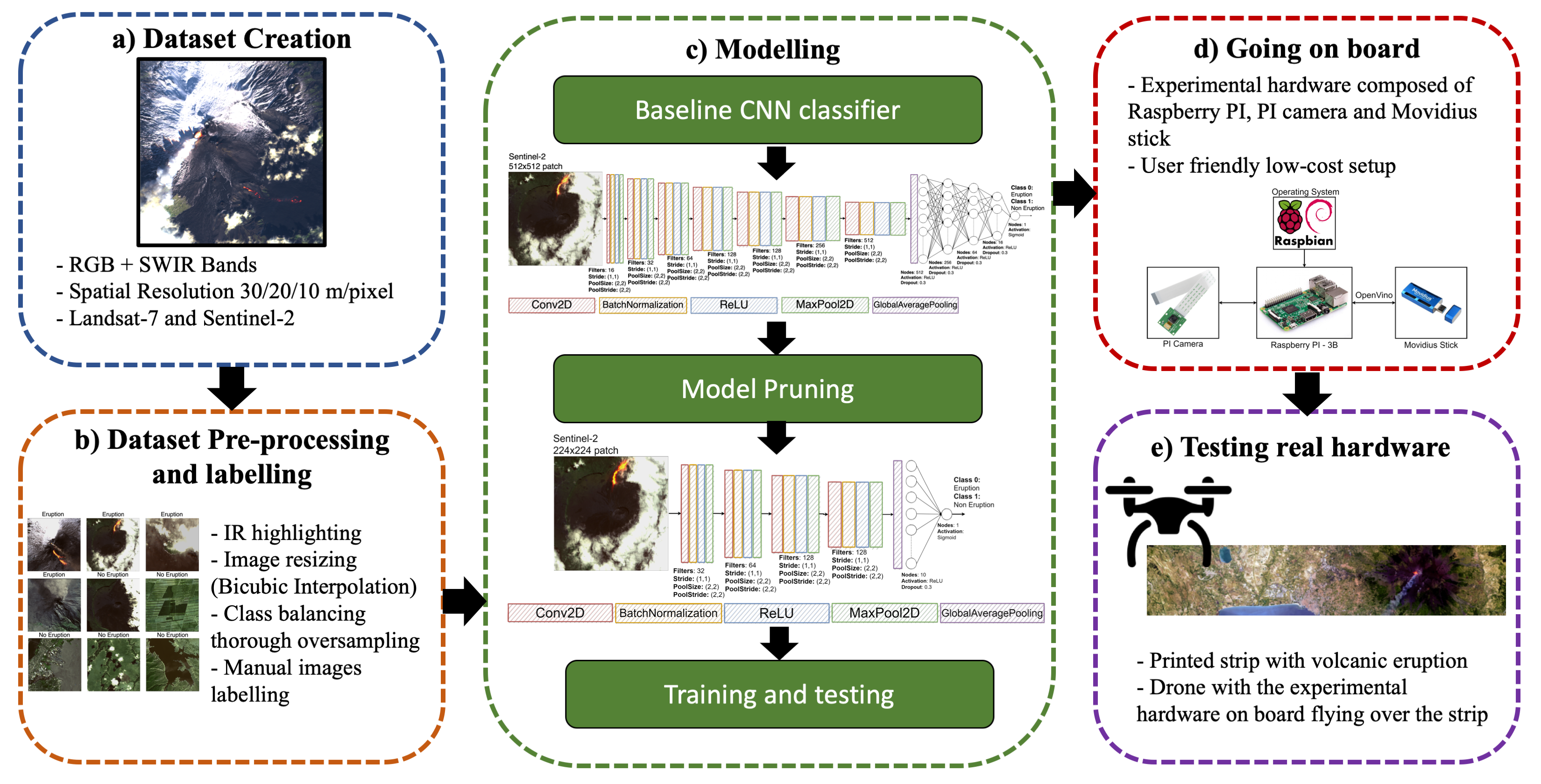
2. Dataset

The chosen use case, as above underlined, focuses on volcanic eruptions by using remote sensing data, hence the first necessary step consists in building the suitable dataset.

Since no ready-to-use data were found to perfectly fit the specific task of this work, a specific dataset was built by using an online catalog of volcanic events including geolocalization information [27]. Satellite images acquired for the place and the date of interest were collected and labeled using the open-access Python tool presented in [28].

2.1. The Volcanic Eruptions Catalog

The dataset has been created by selecting the most recent volcanic eruptions reported in the Volcanoes of the World (VOTW) catalog by the Global Volcanism Program of the Smithsonian Institution. This is a catalog of Holocene and Pleistocene volcanoes and eruptions from the past 10,000 years [27] up to today. An example of information available in the catalog is reported in

Table 1. Sample from the volcanoes of the world (VOTW) [27].

Eruption Start Time	Volcano Name	Latitude (deg)	Longitude (deg)
26 June 2019	Ulawun	−5.050	151.330
24 June 2019	Ubinas	−16.355	151.330
22 June 2019	Raikoke	48.292	153.250
11 June 2019	Piton de la Fournaise	−21.244	55.708
1 June 2019	Great Sitkin	52.076	−176.130

. For the purpose of the dataset creation, the only useful information is the starting date of the eruption, the geographic coordinates and the volcano name. Therefore, this information has been extracted and stored apart.

The images used to create the dataset were collected by using the Landsat-7 and Sentinel-2 products, accessed through Google Earth Engine(GEE) [29]. Specifically, Landsat-7 images have been downloaded considering the period 1999–2015, whereas Sentinel-2 images are related to the period 2015–2019.

For the Sentinel-2 data, the level 1-C was selected, comprising 13 spectral bands representing TOA (Top Of Atmosphere) reflectance scaled by 10,000 and 3 QA bands, including a bitmask band with cloud mask information. The only product of Landsat-7 available in the GEE Catalog is instead level 2.

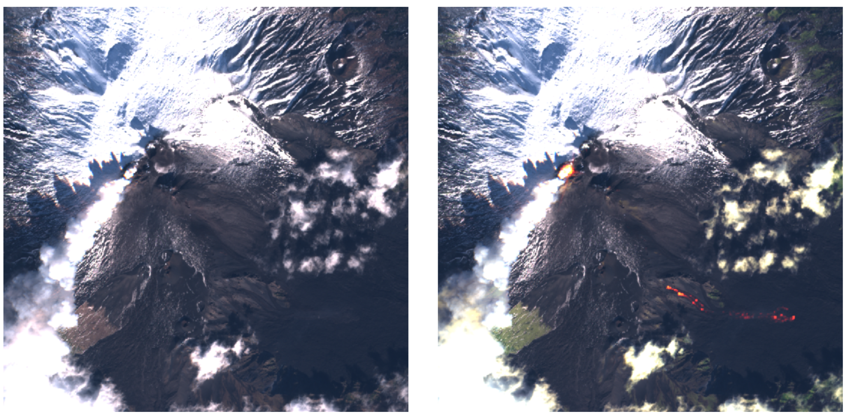
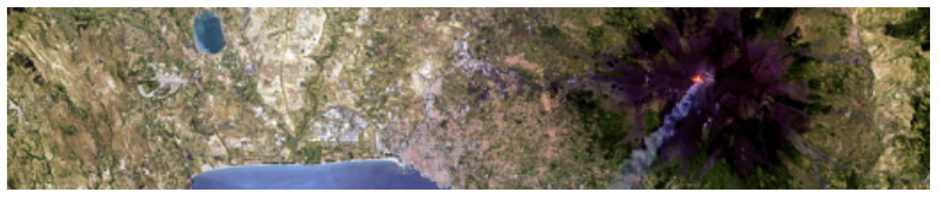
It is worth to underline that, even though the authors have limited this research to Landsat-7 and Sentinel-2, as they cover the entire period of interest, the same approach can be extended to other remote sensing optical products presenting the same bands required for this study, e.g., blue, green, red, and the two SWIR (short-wave infrared) bands located approximately at 1650 nm and 2200 nm. The SWIR bands have been considered in order to better locate and inspect the volcanic eruptions. Indeed, volcanic eruptions can be easily located in RGB wavelengths when they are captured by the satellite camera during the eruptive event, which however is not always the case. After the eruption, the initially red lava gets darker and darker, even though its temperature remains very high. In order to highlight high temperature soil, infrared bands have to be included. The extension to SWIR radiometer data for the volcanic eruption detection will be also examined in order to improve the dataset since the presence of $S{O}_2$ (included in volcanic ejecta) can be in this way identified at an early-stage.

It is worthy to highlight that there are some differences between the Sentinel-2 and Landsat-7 products, both in terms of spatial resolution and bandwidths, as shown in

Table 2. Description of Landsat-7 bands.

Band Name	Description	Wavelength (nm)	Bandwidth (nm)	Spatial Resolution (m)
B1	Blue	485	70	30
B2	Green	560	80	30
B3	Red	660	70	30
B5	SWIR 1	1650	200	30
B7	SWIR 2	2220	260	30

and

Table 3. Description of Sentinel-2 bands.

Band Name	Description	Wavelength (nm)	Bandwidth (nm)	Spatial Resolution (m)
B2	Blue	496.6 (S2A)/492.1 (S2B)	66	10
B3	Green	560 (S2A)/559 (S2B)	36	10
B4	Red	664.5 (S2A)/665 (S2B)	31	10
B11	SWIR 1	1613.7 (S2A)/1610.4 (S2B)	91 (S2A)/94 (S2B)	20
B12	SWIR 2	2202.4 (S2A)/2185.7 (S2B)	175 (S2A)/185 (S2B)	20

. These differences will be addressed in the next sections.

2.2. Data Preparation and Manipulation

Satellite data have been downloaded with the above cited tool [28] that allows to automatically create small patches of images. For this work, the obtained patches cover an overall area of 7.5 km².

After downloading the data, some pre-processing procedures have been applied. Firstly, the images have been resized to $512\times 512$ pixels using the Bicubic Interpolation method of Python OpenCV. This procedure mitigates the difference of spatial resolution between Sentinel-2 and Landsat-7. Secondly, infrared bands are combined with RGB bands, in order to visually highlight the color of the volcanic lava, regardless of its color (which is typically red during the eruption and darker a few hours later). Finally, in the experimental phase the proposed algorithm has been adapted and deployed on a Raspberry PI board with a PI camera [30]. Since the PI camera only acquires RGB data, the bands’ combination has become necessary to simulate RGB-like images. The bands’ combination for highlighting IR spectral answers is given by the equations [31]:

$$\mathrm{RED}={\alpha }_1·B4+max(0,\mathrm{SWIR}2-0.1)$$

(1)

$$\mathrm{GREEN}={\alpha }_2·B3+max(0,\mathrm{SWIR}1-0.1)$$

(2)

$$\mathrm{BLUE}={\alpha }_3·B2$$

(3)

Namely, red and green bands are mixed with SWIR1 and SWIR2 bands, in order to enhance the pixels with high temperature. The multiplicative factor ${\alpha }_x$ is used to adjust the scale of the image and it is set to 2.5. In practice, the infrared bands change the red and green bands, so that the heat information is highlighted and visible to the human eye. In this way, it was possible to create a quantitatively correct dataset since, during the labeling, the eruptions were easily distinguishable from non-eruptions. In Figure 1 the difference between a simple RGB image and the one highlighting IR is shown.

2.3. Dataset Expansion

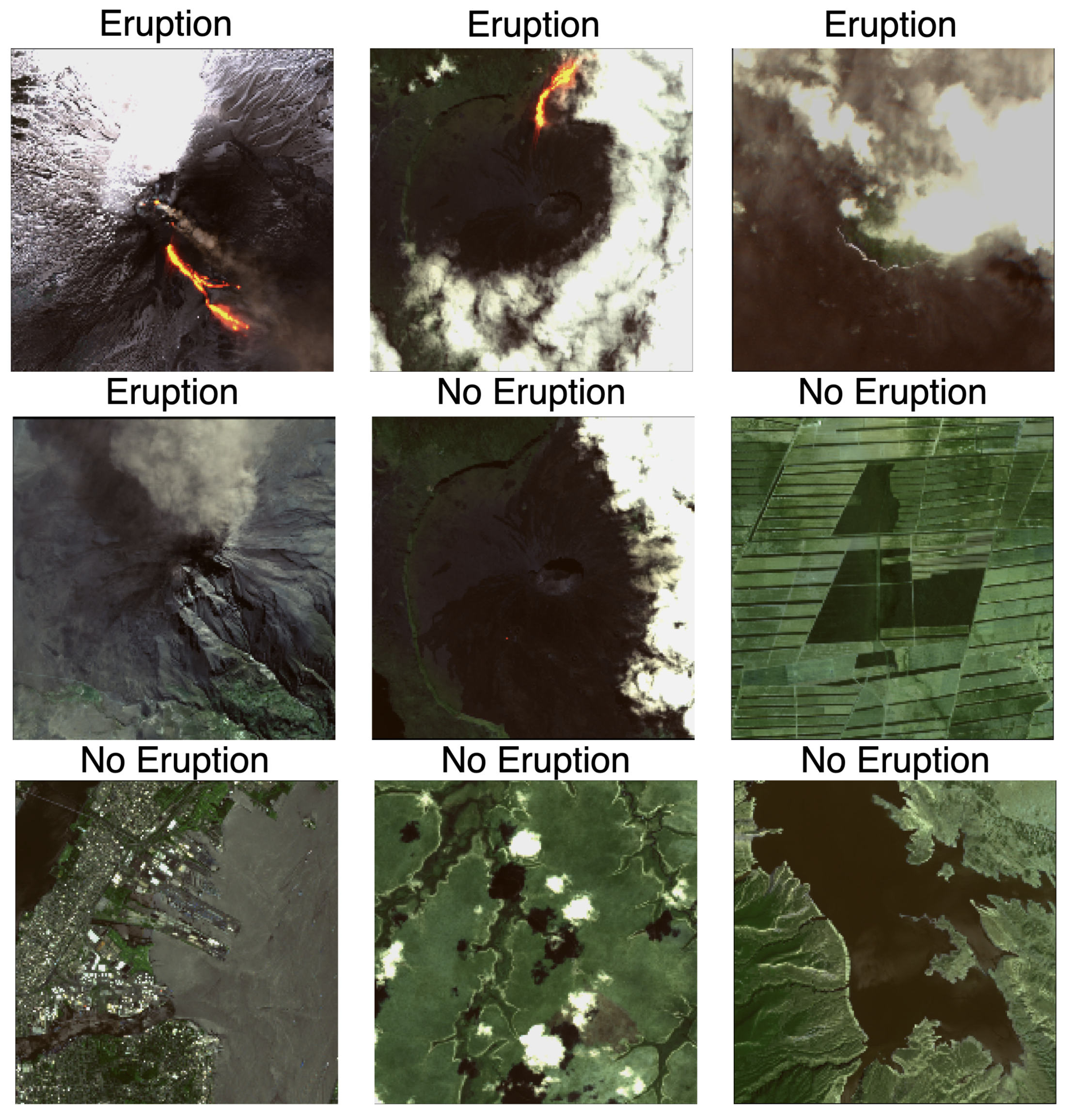
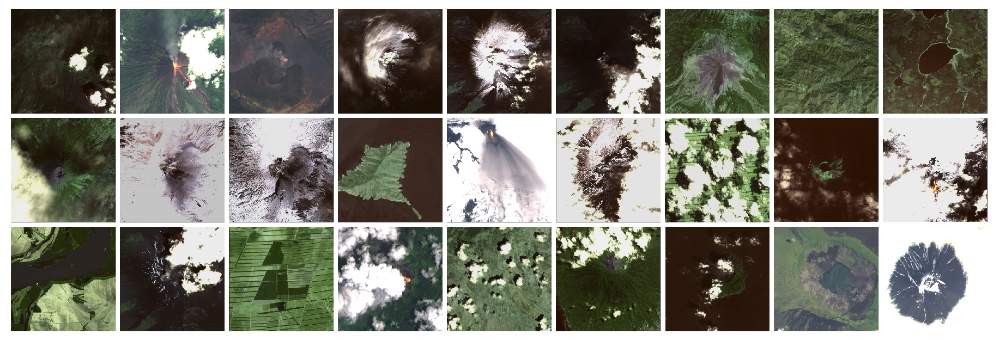
Since the task addressed in this paper is a typical binary classification problem, images have been downloaded in order to fill both the eruption and the no-eruption classes. To have a high variability and to reach better results the no-eruption images have been downloaded by focusing on five sub-classes: (1) non-erupting volcanoes, (2) cities, (3) mountains, (4) cloudy images and (5) completely random images. The presence of cloudy images is really important, in order to make the CNN learn to distinguish between eruption smoke and clouds. An example of comparison is shown in Figure 2.

The same pre-processing step has been applied to the new data, since in the deep learning context a homogeneous dataset is preferable for reducing the sensitivity of the model to variations in the distribution of the input data [32,33]. The final dataset contains 260 images for the class eruption and 1500 for the class non-eruption. Due to the type of event analyzed, the dataset appears to be unbalanced, as an acquisition with an eruption is a rare event. The problem of the imbalanced dataset is addressed in the next sections.

In Figure 3 some images from the downloaded and pre-processed dataset are shown. Moreover, it is worth to highlight that the final dataset has been made freely available on GitHub [34].

3. Proposed Model

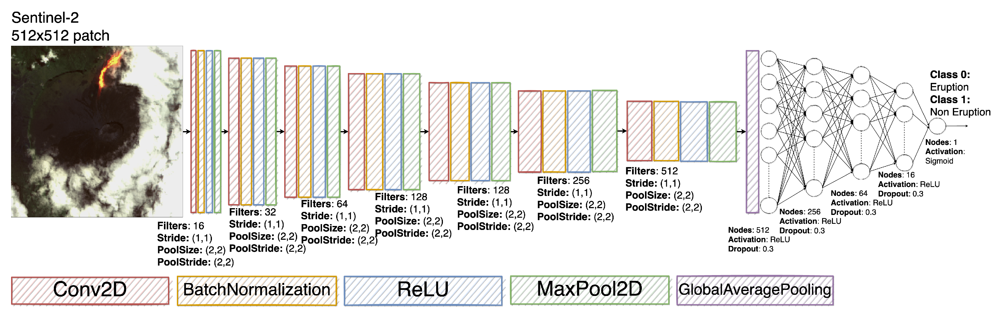
The detection task has been addressed by implementing a binary classifier where the first class is assigned to images with eruptions and the second one addresses all the other scenarios. The overall CNN architecture is shown in Figure 4. The proposed CNN can be divided in two sub-networks: the first convolutional network is responsible for the features extraction and the second fully connected network is responsible for the classification task [32,33,35]. The architecture used to build from scratch the proposed model can be derived from classical models frequently used by the Computer Vision (CV) community, for example the AlexNet/VggF [36] or the LeNet-5 [37]. The main differences with the these architectures are in the number of convolutional and dense layers and in the use of a Global Average Pooling layer instead of a classical flatten layer.

The first sub-network consists of seven convolutional layers, each one followed by a batch normalization layer, a ReLU activation function and a max pooling layer. Each convolutional layer has a stride value equal to (1,1) and an increasing number of filters, from 16 to 512. Each max pooling layer (with size (2,2) for both kernel and stride) halves the feature map dimension. The second sub-network consists of five fully-connected layers, where each layer is followed by a ReLU activation function and a dropout layer. In this case the number of elements of each layer decreases. In the proposed architecture the two sub-networks are connected with a global average pooling layer that, compared to a flatten layer, drastically reduces the number of trainable parameters, speeding up the training process.

3.1. Image Loader and Data Balancing

Given the nature of the analyzed hazard, the dataset results unbalanced. An unbalanced dataset, with a number of examples of one class much greater than the other, will lead the model to recognize only the dominant class. To solve this issue, an external function called Image Loader from the Phi-Lab ai4eo.preprocessing library has been used [38].

This library allows the user to define a much more efficient image loader than the already existing Keras version. Furthermore, it is possible to implement a data augmentator that allows the user to define further transformations. The most powerful feature of this library is the one related to the balancing of the dataset through the oversampling technique. In particular, each class is weighted independently using a value based on the number of the class samples. The oversampling mechanism acts on the minority class, in this case the eruption class, by applying the data augmentation. This latter generates new images by applying transformations of starting images (e.g., rotations, crops, etc.) until the minority class reaches a number of samples equals to the majority class. This well known strategy [39], increases the computational cost for the training but helps the classifier, during the learning phase, not to strengthen on a specific class, since after this procedure it will have an equal number of data available for each class.

3.2. Training

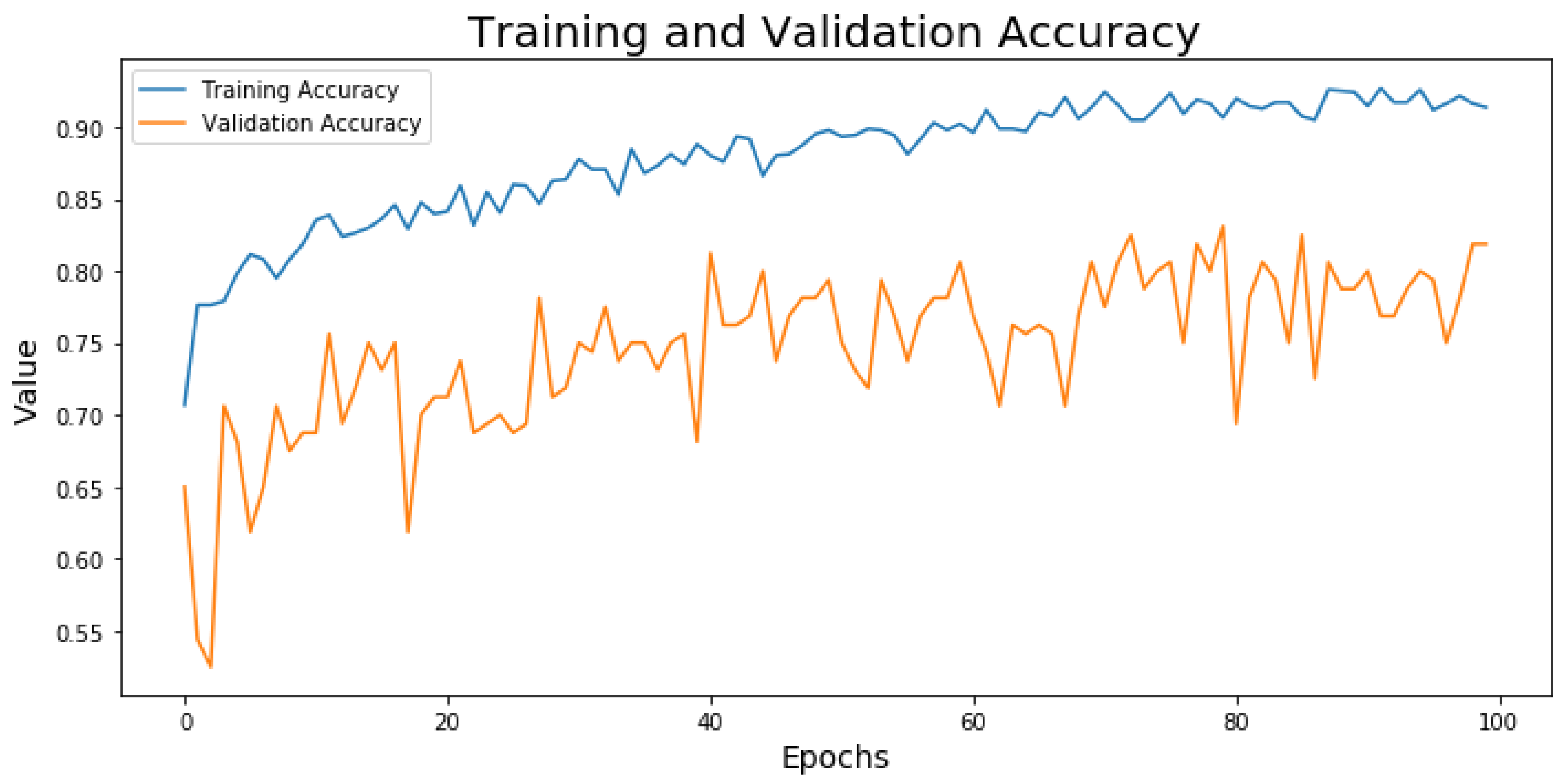
During the training phase, for each epoch the error between the real output and the prediction is calculated both on the training and on the validation datasets. The metric used for the error has been the accuracy and it is worth to underline that this metric works precisely only if there is an equal number of samples belonging to both classes. The model has been trained for 100 epochs, using the Adam optimizer and the binary cross-entropy as loss function.

The training dataset is composed of 1215 examples, among which 334 are with eruptions and 818 are without eruptions. The validation dataset contains 75 eruption samples and 94 no eruption images. Both datasets have been subjected to the data augmentation and to the addition of white Gaussian noise to each channel to increase the robustness of the model and to solve the spectral diversity between Sentinel-2 and Landsat-7.

The model was trained on the Google Colaboratory platform, where each user can count on: (1) a GPU Tesla K80, having 2496 CUDA cores, compute 3.7, 12G GDDR5 VRAM, (2) a CPU single core hyper threaded i.e., (1 core, 2 threads) Xeon Processors @2.3 Ghz (No Turbo Boost), (3) 45MB Cache, (4) 12.6 GB of available RAM and (5) 320 GB of available disk. With such an architecture, each training epoch required about 370 s. The trends of the accuracy on training and validation dataset are shown in Figure 5.

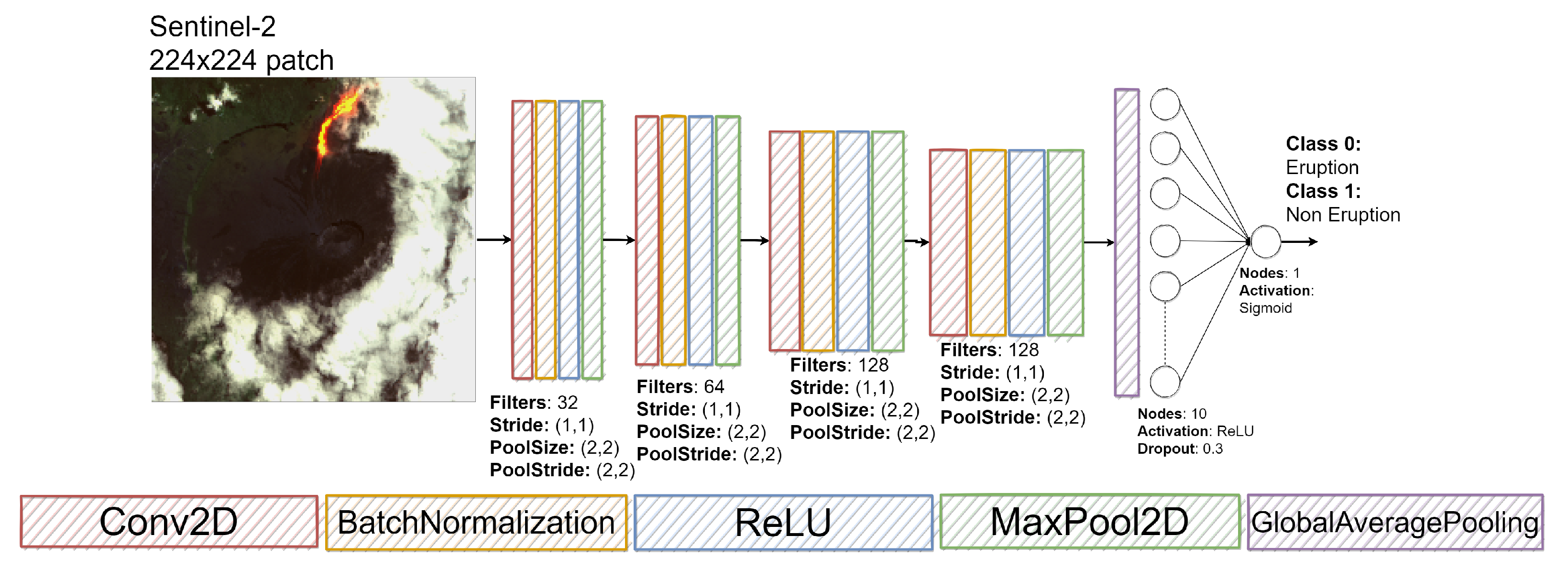
3.3. Model Pruning

Since the final goal is to realize a model to be uploaded on an on-board system, its optimization is necessary in terms of network complexity, number of parameters and inference execution time. The choice of using a small chip led to limitations of executing the specific classification model, due to the chip’s limited elaboration power, thus it was necessary to derive a proper model. Model pruning was driven by the goal of minimizing inference time, because its value represents a strict requirement for our experimental setup. An alternative interesting procedure for model pruning and optimization has been proposed by [40], where authors developed a <1-MB Lightweight CNN detector. Yet, in this manuscript, the work proposed by [12] has been used as a reference paradigm for the on board AI system, since more suitable.

Hence, starting from the first feasible network, a second and smaller network was built by pruning the former one, as shown in Figure 6. The convolutional sub-network has been reduced by removing three layers and the fully connected sub-network has been drastically reduced to only two layers. The choice on the number of layers to remove has been a trade off between the number of network parameters and its capability of extracting useful features. For this reason, the choice relapsed on discarding the last two convolutional layers and the very first one. This choice led to quite good results, revealing a good compromise between memory weight, computational load and performances. The new modified network has shown to be still capable of discriminating or classifying data correctly, with an accuracy of 0.83%.

The smaller model has been trained with the same configuration of the original one. The trends of the training and the validation loss and accuracy functions are shown in Figure 7.

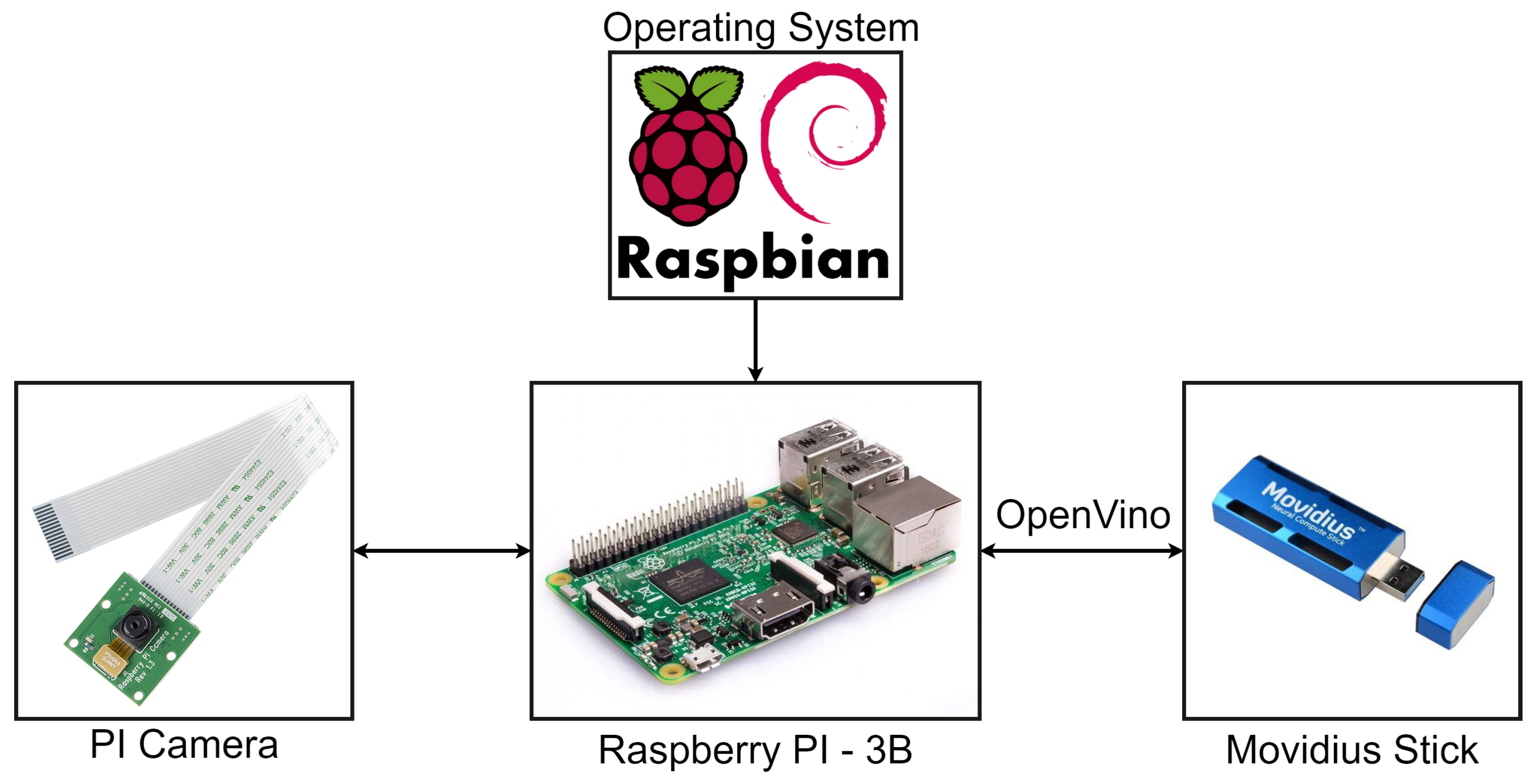
4. Going on Board, a First Prototype

In order to evaluate the proposed methodology, a prototype for running the experimental analysis has been realized. Firstly, the model has been adapted to work with the selected hardware and to carry out the on board volcanic eruption detection. The hardware is composed of a drone, used a RS platform, of a Raspberry PI used as main on board computer, a PI camera used as acquiring sensor and a Movidius stick used as Deep Learning accelerator [41,42,43]. The experimental setup is shown in Figure 8. The description of the architecture of the drone system is out of the scope of this work since the drone has only been used for simulation purposes, thus its subsystems are not included in the schematic.

The peculiarity of the proposed system, apart from the drone, is the availability of the low-cost user-friendly components used to realize it. Moreover the components are almost ready to use and are easy to install. These aspects allow the proposed system to be easily replicable, allowing interested researchers to repeat the experiments proposed in this manuscript.

The functiong pipeline is handled by the Raspberry PI, with the Raspbian Operating System (OS), that is the on board computer. This board will process the images acquired through the PI camera and send them to the Movidius Stick in order to run the classification algorithm, based on the selected CNN model.

In the next subsections, all the components used for the experimental setup are briefly described, to give the reader some useful information about their main characteristics.

4.1. Raspberry PI

The Raspberry adopted for this use case is the Raspberry Pi 3 Model B, the earliest model of the third-generation Raspberry Pi.

Table 4. Raspberry PI 3 specifications.

Component	Specifications
Processor	Quad Core 1.2 GHz Broadcom BCM2837 64bit CPU 1GB RAM
Wireless systems	BCM43438 wireless LAN and Bluetooth Low Energy (BLE) on board
Hardware sysetms	100 Base Ethernet
Hardware connectors	40-pin extended GPIO
USB Ports	4 USB 2.0 ports
Video Ports (1)	4 Pole stereo output and composite video port
Video Ports (2)	Full size HDMI
Camera Port	CSI camera port for connecting a Raspberry Pi camera
Display Port	DSI display port for connecting a Raspberry Pi touchscreen display
External Memory Port	Micro SD port for loading your operating system and storing data
Power Supply Poprt	Upgraded switched Micro USB power source up to 2.5A

shows its main specifications.

4.2. Camera

The Raspberry Pi Camera Module v2, is a high quality 8-megapixel Sony IMX219 image sensor custom designed add-on board for Raspberry Pi, featuring a fixed focus lens. It is capable of 3280 × 2464 pixel static images, and supports 1080p30, 720p60 and 640 × 480p90 video. The camera can be plugged using the dedicated socket and CSi interface. The main specifications for PI camera are listed in

Table 5. Raspberry Pi RGB camera specifications.

Component	Specifications
Focus	Fixed focus lens on board
Resolution	8 megapixel native resolution sensor
Frame size	3280 × 2464 pixel static images
Video Support	Supports 1080p30, 720p60 and 640 × 480p90 video
Physical Dimension	Size 25 mm × 23 mm × 9 mm
Weights	Weight just over 3 g

.

4.3. Movidius Stick

The Intel Movidius Neural Compute Stick is a small fanless deep learning USB drive designed to learn AI programming. The stick is powered by the low power high performance Movidius Visual Processing Unit. It contains an Intel Movidius Myriad 2 Vision Processing Unit 4GB. The main specifications are:

• Supporting CNN profiling, prototyping and tuning workflow
• Real-time on device inference (Cloud connectivity not required)
• Features the Movidius Vision Processing Unit with energy-efficient CNN processing
• All data and power provided over a single USB type A port
• Run multiple devices on the same platform to scale performance

4.4. Implementation on Raspberry and Movidius Stick

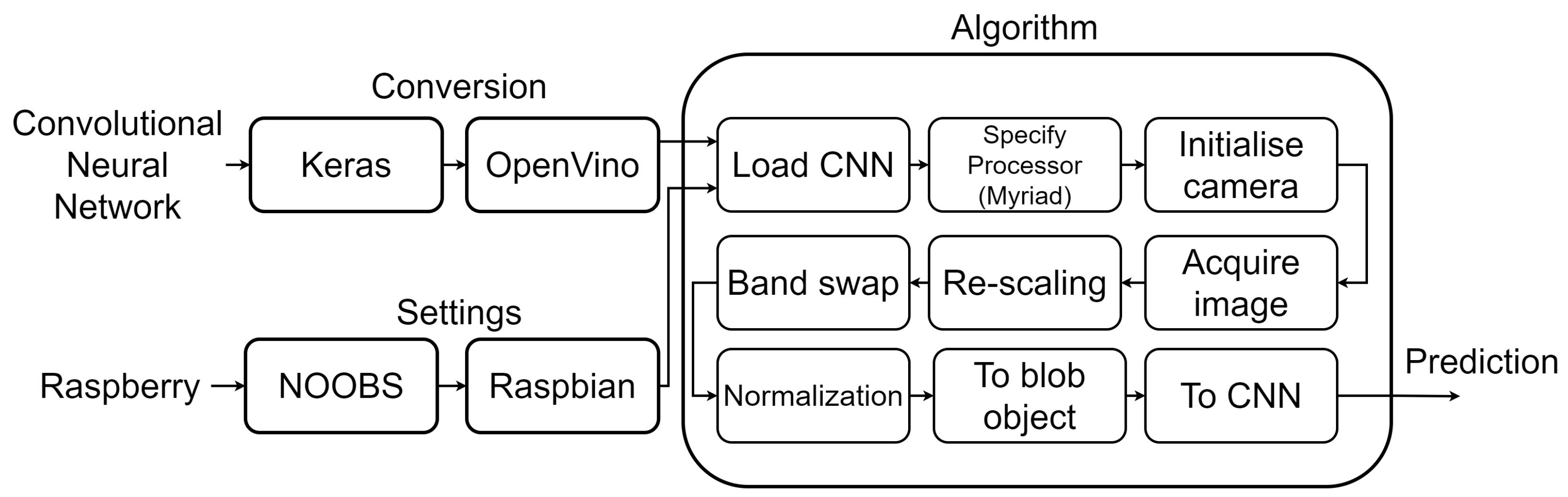
This subsection summarizes the pipeline for running experiments and for implementing the software components on the hardware setup.

In order to run the experiments with the Raspeberry PI and the Movidius Stick, two preliminary steps are necessary: (1) the CNN must be converted from the original format (e.g., Keras model) to an OpenVino format, using the OpenVino library; (2) an appropriate operating system must be install on the Raspberry (e.g., the Rasbian OS through the NOOBS installer). The implementation process is schematized in Figure 9.

OpenVINO Library

For deep learning, the current Raspberry PI hardware is inherently resource constrained. The Movidius Stick allows faster inference with the deep learning coprocessor that is plugged into the USB socket. In order to transfer the CNN on the Movidius, the network should be optimized, using the OpenVINO Intel library for hardware optimized computer vision.

The OpenVINO toolkit is an Intel Distribution and is extremely simple to use. Indeed, after setting the target processor, the OpenVINO-optimized OpenCV can handle the overal setup [44]. Based on CNN, the toolkit extends workloads across Intel hardware (including accelerators) and maximizes performance by:

• enabling deep learning inference at the edge
• supporting heterogeneous execution across computer vision accelerators (e.g., CPU, GPU, Intel Movidius Neural Compute Stick, and FPGA) using a common API
• speeding up time to market via a library of functions and pre-optimized kernels
• including optimized calls for OpenCV.

After implementation on Raspberry and Movidius, the models were tested by acquiring images using a drone flying over a print made with Sentinel-2 data of an erupting volcano, as shown in Figure 10. The printed image has been processed with the same settings used for the training and validation dataset.

5. Results and Discussion

5.1. Training on the PC

The models’ performances have been computed on the testing dataset. The big extended model reached an accuracy of 85%, while the smaller and lighter model reached an accuracy of 83%.

In Figure 11, as an example, a subset of the testing dataset is shown, while in

Table 6. Model results on testing dataset.

Column	Row 1		Row 2		Row 3
	Ground Truth	Predicted	Ground Truth	Predicted	Ground Truth	Predicted
1	1.00	0.13	0.00	0.03	0.00	0.00
2	1.00	0.99	1.00	0.99	1.00	0.99
3	1.00	0.99	1.00	0.99	0.00	0.00
4	1.00	0.95	0.00	0.00	1.00	0.99
5	1.00	0.98	1.00	0.99	0.00	0.00
6	1.00	0.99	1.00	0.99	0.00	0.02
7	0.00	0.00	0.00	0.00	1.00	0.99
8	0.00	0.00	0.00	0.26	0.00	0.88
9	0.00	0.00	1.00	0.99	0.00	0.01

the corresponding ground truth and prediction labels are reported. A low value for a predicted label indicates a low probability of eruption, so the image is classified as no eruption; a high value for a predicted label indicates a high probability of eruption, so the image is classified as eruption; a value next to 0.5 indicates an inconclusive prediction. Since the problem is a binary classification, a threshold value of 0.5 was selected to identify the class based on the prediction: a value lower that 0.5 was rounded to 0 (non-eruption class), while a value higher than the 0.5 was rounded to 1 (eruption class).

The performances have been computed also for the second model, the one obtained after the pruning process. The same samples shown in Figure 11 have been used to make the comparison with the original model.

Table 7. Small model results on the testing dataset.

Column	Row 1		Row 2		Row 3
	Ground Truth	Predicted	Ground Truth	Predicted	Ground Truth	Predicted
1	1.00	0.99	0.00	0.56	0.00	0.08
2	1.00	0.99	1.00	0.94	0.00	0.00
3	1.00	0.99	1.00	0.97	0.00	0.01
4	1.00	0.01	0.00	0.01	0.00	0.64
5	1.00	0.99	1.00	0.99	0.00	0.00
6	1.00	0.97	1.00	0.99	1.00	0.97
7	0.00	0.00	0.00	0.99	1.00	0.00
8	0.00	0.99	0.00	0.00	0.00	0.00
9	0.00	0.00	1.00	0.00	0.00	0.00

shows the results.

The training of the two proposed CNNs has been made with the same machine and for 100 epochs each. As stated before, the platform used for the training is Google Colaboratory that presents a GPU xTesla K80, having 2496 CUDA cores, compute 3.7, a 12 Gb (11.439 Usable) GDDR5 VRAM, a CPU 1xsingle core hyper threaded i.e., (1 core 2 threads) Xeon Processor 2.3 Ghz (No Turbo Boost), 45 Mb of Cache, 12.6 Gb of RAM and 320 Gb of available disk. Details about models size and training time can be found in

Table 8. Performances comparison considering the big and the small models.

	Big Model	Small Model
Trainable Parameter	2,136,385	243,541
Non-trainable Parameter	2272	704
Model weight	24.6 Mb	1.9 Mb
Training Time	∼10 h	∼3 h

, while details about models scores and inference time can be found in

Table 9. Performances comparison considering the big and the small models (in details).

Score	Big Model	Small Model
True Positive (TP)	0.85	0.83
True Negative (TN)	0.85	0.83
False Positive (FP)	0.15	0.17
False Negative (FN)	0.15	0.17
Overall accuracy	0.85	0.83
Precision	0.85	0.83
Recall	0.85	0.83
F1 Score	0.85	0.83
images/second	1	7

.

5.2. Results on the Movidius

The confusion matrix, the classifications scores and the architecture computational speed, for the two models, are reported in Table 9, where is evident that the performances in terms of good prediction are slightly changed after the model pruning, but the most important aspect is that the images per second that the model and the hardware can handle is increased from 1 to 7.

The values of accuracy, precision, recall and F1 score reported in Table 9 are defined as follows,

$$\begin{array}{cc}\hfill \mathrm{Accuracy}=\frac{TP+TN}{TP+FP+FN+TN},& \mathrm{Precision}=\frac{TP}{TP+FP}\hfill \\ \hfill \mathrm{Recall}=\frac{TP}{TP+FN},& \mathrm{F}1\mathrm{Score}=2\frac{\mathrm{Recall}\ast \mathrm{Precision}}{\mathrm{Recall}+\mathrm{Precision}}\hfill \end{array}$$

(4)

where $TP,TN,FP,FN$ are the number of True Positive cases, True Negative cases, False Positive cases, and False Negative cases, respectively.

The results shown in Table 9 are fundamental, since good performances are maintained and the small model can allow to respect the constraints imposed by the dynamics and mission of the drone used in the experimental phase. It is worth to underline that, although the Raspberry system has to carry out several operations: image acquisition, image pre-processing, communication with the movidius stick, inference, wireless communication with the on ground station, and so on, despite the limited amount of processing power, the overall inference time has been reduced by a factor of 7.

This result is perfectly transferable to the satellite domain, obviously considering the constraints imposed by these platforms. The results are promising, demonstrating the correctness of the proposed pipeline and justifying further analysis and investigation.

6. Conclusions

This work aimed to present a first workflow on how to develop and implement an AI model to be suitable for being carried on board satellites for Earth Observation. In particular, two detectors of volcanic eruptions have been developed and discussed.

AI on board is a very challenging field of research which has seen the ESA as a pioneer in moving the first steps with the Phisat-1 satellite launched on September the 3rd 2020. The possibility to process data on board a satellite can drastically reduce the time between the image acquisition and its analysis, completely deleting the time for downlinking and reducing the total latency. In this way, it is possible to produce fast alerts and interventions when hazardous events are going to happen.

A prototype and a simulation process, keeping a low-cost kind of implementation, were realized. The experiment and the development chain were completed with commercial and ready-to-use hardware components, and a drone was also employed for simulations and testing. The AI processor had no problem in recognizing the eruption in the printed image used for testing. The results are encouraging, showing that even the pruned model can reach a good performance in detecting the eruptions. Further studies will help to understand possible extensions and improvements.