Axle Configuration and Weight Sensing for Moving Vehicles on Bridges Based on the Clustering and Gradient Method

Abstract

Traffic information, including vehicle weight and axle spacing, is vital for bridge safety. The bridge weigh-in-motion (BWIM) system remotely estimates the axle weights of moving vehicles using the response measured from instrumented bridges. It has been proved more accurate and durable than the traditional pavement-based method. However, the main drawback of conventional BWIM algorithms is that they can only identify the axle weight and the information of axle configuration (the number of axles and axle spacing) is required to be determined using an extra device in advance of the weight identification procedure. Namely, dedicated sensors (pressure-sensitive sensors placed on the deck surface or under the soffit of a bridge) in addition to weighing sensors must be adopted for identifying the axle configuration, which significantly decreases the utility, feasibility, and economic efficiency of BWIM technology. In this study, a new iterative procedure simultaneously identifying axle spacing as well as axle weights and gross weights of vehicles is proposed. The novel method is based on k-means clustering and the gradient descent method. In this method, both the axle weight and the axle location are obtained by using the same global response of bridges; thus the axle detectors are no longer required, which makes it economical and easier to be implemented. Furthermore, the proposed optimization method has good computational efficiency and thus is practical for real-time application. Comprehensive numerical simulations and laboratory experiments based on scaled vehicle and bridge models were conducted to verify the proposed method. The identification results show that the proposed method has good accuracy and high computational efficiency in axle spacing and axle weight identification.

1. Introduction

Operational traffic load data are vital for the assessment and maintenance of transportation infrastructure [1,2], such as the axle spacing, axle weight, and gross weight of moving vehicles. In addition, it is of significance to monitor moving vehicles on bridges for traffic management and load limit enforcement [3,4]. The bridge weigh-in-motion (BWIM) system, conceptually proposed first by Moses in the 1970s [5], uses an instrumented bridge as a scale to weigh vehicles passing the bridge at a normal highway speed, which provides an effective procedure for reliable measurement of the axle spacing, axle weights, and gross vehicle weights of trucks without interrupting the regular traffic.

Moses’ original BWIM algorithm or its derivatives are still the theoretical basis of state-of-the-art commercial BWIM systems [4], where the axle weights of vehicles can be determined by minimizing the square of the Euclidean distance of measured bridge responses and those by using the influence line method. Based on Moses’ algorithm, several other approaches have been developed in the past, aiming to improve its accuracy and robustness [6,7]. Two comprehensive state-of-the-art reviews on existing BWIM algorithms and their recent applications were composed by Yu et al. [8] and Lydon et al. [9], respectively.

For the majority of existing BWIM algorithms, the number of axles and axle locations (i.e., axle spacing) of the vehicle is required when calculating the axle weights. In the first BWIM system, Moses identified vehicle axles through tape switches installed on the top of the bridge surface [5]. Although this method is quite simple and accurate, it usually causes disruptions to traffic and has a short service life since the sensors are directly bearing the massive truck tire loads. Recently, due to the development in sensing material and fabrication techniques, some more durable sensors were invented, which makes the direct method a useful option for portable applications [10]. Therefore, a new conception of a nothing-on-road (NOR) BWIM system and a free-of-axle-detector (FAD) technology were proposed to avoid the necessity of directly installing sensors on the road surface [11]. In the FAD scheme, sensors are attached to the bottom of the bridge deck to monitor vehicle axles by measuring bridge local strains. These FAD sensors have better durability; however, they are only suitable for specific types of bridges and are sensitive to the deck thickness, road surface roughness, and vehicle lateral position [11,12,13].

In the past decades, some researchers have attempted to identify the vehicle speed and axle spacing by directly using the global flexural strain information acquired from the weighing sensors. By calculating the second differential of the bridge bending response, Wall et al. [14] managed to obtain the information of vehicle velocity and axle configuration. It was also found that the vehicle axles can be identified by applying peak analysis on the time history of flexural strains, though some axles might occasionally become unidentifiable [15].

The shear-force-based method was recently proved to be an effective and efficient axle detection strategy [16]. In this method, shear strain gauges are attached to the web plate of a bridge in two sections to measure the shear strain of the bridge under the load of moving vehicles. Sudden changes in the time histories of the shear strains are then used to monitor axles. Bao et al. [17] conducted field tests to detect the speed and axle spacing of vehicles. In the study, the axle weight and gross weight of vehicles were also estimated from the global shear strain. Field tests by Kalhori et al. [15] found that compared to the shear strain measured at mid-span and quarter-span, more accurate results of axle detection can be obtained by using the shear strain measured near the end supports of the bridge. However, this method is only suitable for those bridges whose web plate is accessible for shear sensor installations. Furthermore, apart from the necessary weighing sensors in a BWIM system, it still requires additional shear strain sensors.

Wavelet transformation, a powerful signal processing tool, was also applied to enhance the accuracy of axle detection. Dunne et al. [18] and Chatterjee et al. [19] successfully obtained vehicle axle information, even for closely spaced axles within tandem or tridem axle groups, through wavelet transformation. Yu et al. [20] proposed a vehicle axle identification method using only the global signal from the weighing sensors based on wavelet transformation. It was also noted that wavelet analysis-based techniques were unstable in certain circumstances where errors existing in the raw data could be amplified in outputs [9]. Computer vision, as a new technology, was also adopted for vehicle and axle monitoring. Ojio et al. [21] first proposed the contactless BWIM concept. In their scheme, one traffic camera was used for vehicle and wheel tracking, and another high-resolution camera was used for monitoring the displacement of the bridge. Xia et al. [22] developed an efficient infrastructure safety oriented BWIM system by composing surveillance cameras and multiple strain sensors. The drawback of this method is that a huge computational resource is needed for high-speed video capturing and real-time image processing; thus it is not economically efficient for field deployment yet.

More recently, He et al. [23] proposed a novel virtual simply supported beam method (VSSB) that managed to identify vehicle axles in a completely different perspective. In [23], the vehicle axles were directly obtained from so-called isolated strains, which are the calculation results of strain signals measured from four different longitudinal positions of the bridge. Chen et al. [24] developed a BWIM system using long-gauge fiber sensors based on the second differential of the bridge strain response, which is equivalent to the isolated strain, and achieved good performance in field tests. Deng et al. [25] proposed another method in which the difference of the normal strains measured at two sections was considered an approximation or equivalence (with a constant scale) to shear force. This method used the sudden changes in the equivalent shear force to reflect vehicle axles and is considered more advanced than the VSSB method since it reduced the need for total measuring stations from four to three. Compared to the other methods, these methods do not need any complicated signal analysis and are not restricted to certain bridge types or boundary conditions, while the disadvantage is that additional sensors are still required. Hence, the authors recently [26] proposed a virtual axle (VA) method to detect axle spacing and weight all from the same weighing sensors in the same time. The method requires no external axle detector and works well in most scenarios. However, the method uses discretization and exhaust algorithm to search for the exact axle locations and thus can be time-consuming, especially when the discretization resolution was set smaller for better accuracy.

In this study, a new method synchronously detecting the axle weight and spacings of moving vehicles passing over instrumented bridges without preceding knowledge of axle configuration adopting clustering and gradient techniques is proposed. This method uses pre-calibrated bridge influence lines, on-site measured bridge responses, and externally acquired vehicle speed to identify axle spacing and axle weights. Therefore, it is more convenient than the conventional NOR-BWIM systems since it requires no additional devices or sensors for detecting the number of axles and axle spacing in advance. Numerical simulations based on a 3D bridge–vehicle interaction (BVI) system as well as scaled model experiments based on a laboratory vehicle–bridge vibration test platform were conducted in order to validate the proposed method.

2. Methodology

2.1. Moses’ Axle Weight Estimating Algorithm

The response of a bridge at sampling time t under the load of a single moving vehicle axle can be determined by multiplying the axle weight and the ordinate of influence line function at the location of the axle:

$$S_i(t)=I\left(x_i(t)\right)\cdot P_i$$

(1)

where S_i is the bridge response under the load of the i-th axle, I(x) is the influence line function of the bridge response relative to the load position x, and x_i and P_i are the location and the weight of the i-th axle, respectively. Then, the overall response of the bridge under the load of the vehicle can be assembled by summing all individual responses induced by each axle of the vehicle:

$$S(t)={\displaystyle \sum _{i=1}^N{S}_i(t)=}{\displaystyle \sum _{i=1}^{N}I\left(v\cdot t-x_i^0\right)\cdot P_i}$$

(2)

where v is the speed of the vehicle and $x_i^0$ is the distance from the i-th axle to the first axle.

In contrast, the bridge response can be directly acquired from the sensors by using data acquisition equipment, which is denoted as $S^{\prime }(t)$. Theoretically, the best estimation of the weight of the axles will make the theoretical response S(t) and the measured response $S^{\prime }(t)$ as close as possible. The Euclidean distance of the theoretical and measured response series is

$$E(P)={\Vert {S-S}^{\prime }\Vert }_2^2={\displaystyle \sum _{k=1}^K{\left(S(t_k)-S^{\prime }(t_k)\right)}^2}$$

(3)

where S and S′ are the time histories of theoretical and measured response, respectively, sampled at serial time points $t_k=T_0+k\cdot T_s$, $k=1,2,\dots ,K$; ${\Vert \cdot \Vert }_2^2$ denotes the Euclidean norm of a vector; and $P={\left[P_1,P_2,\dots ,P_N\right]}^T$ is the vector of the unknown axle weights, which therefore, can be identified by minimizing the error function (Euclidean distance) via the least square method. It should be marked that the estimation of weight vector P is determined as soon as the axle locations and velocity of the vehicle ($x_i^0$ and v) are given.

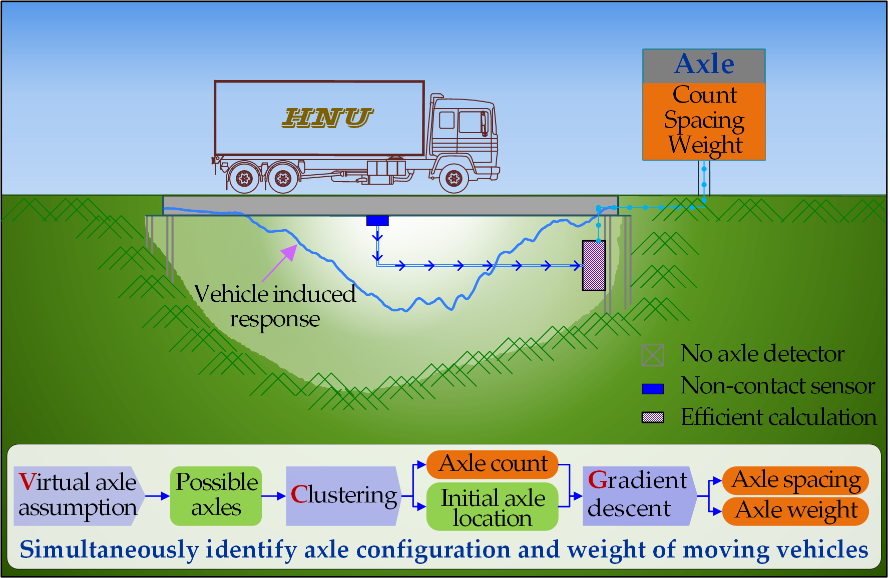
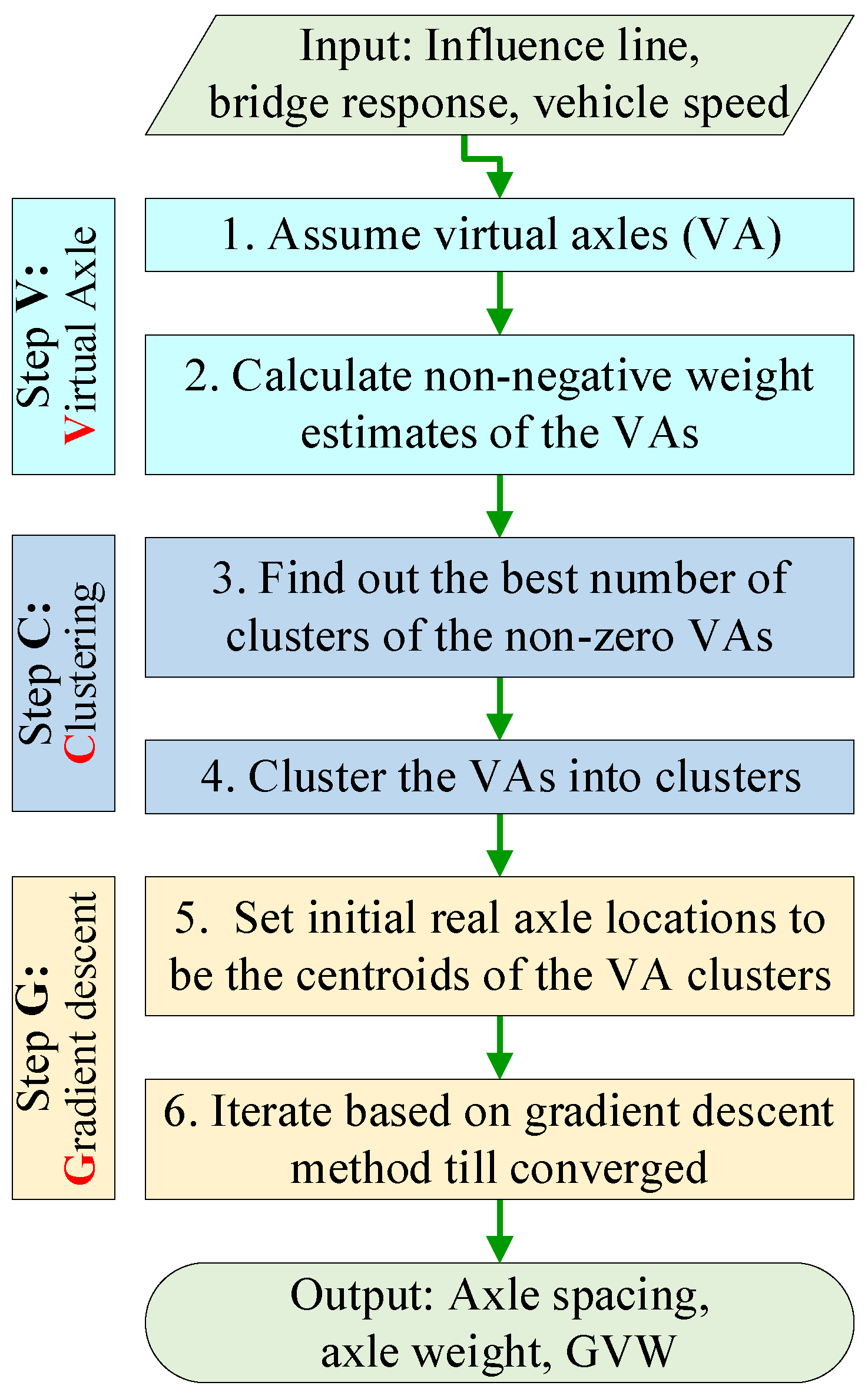
2.2. Overview of the Proposed Optimization Algorithm

In terms of the linear theory assumption, the bridge response under a moving vehicle can be considered as the sum of the response under each axle of the vehicle in the time domain (time lag is relative to axle spacing and vehicle speed). Based on this assumption, Moses’ algorithm and its derivatives formed an objective function relative to axle weight. The axle weight can then be determined using the least square method once the vehicle speed and axle spacing are obtained. However, the main disadvantage of the conventional Moses’ algorithm is the demand for knowing the axle count and axle spacing ahead of the axle weight identification process. To address this issue, an innovative axle-weighing algorithm based on the constraint that the axle weight will not be negative is first introduced. This algorithm calculates the axle weight under the condition that the axle locations are specified. Then, an iterative scheme for simultaneously detecting axle locations (spacing) and axle weights based on the gradient method is presented. Overall, the method proposed in this paper includes three main components, as presented in Figure 1: step V, assume that the truck consists of evenly spaced virtual axles and find out their non-negative estimation; step C, cluster the non-zero virtual axles into several axle sets using the k-means method and the elbow method [27]; step G, take the centroid locations of the axle clusters as initial values and repeat the gradient-descent-based iteration scheme presented in later sections until convergence in order to find out the actual axle locations, axle weights, and gross vehicle weight (GVW). The proposed method is therefore hereafter referred to as the VCG method for convenience, and the details will be introduced in the following sections.

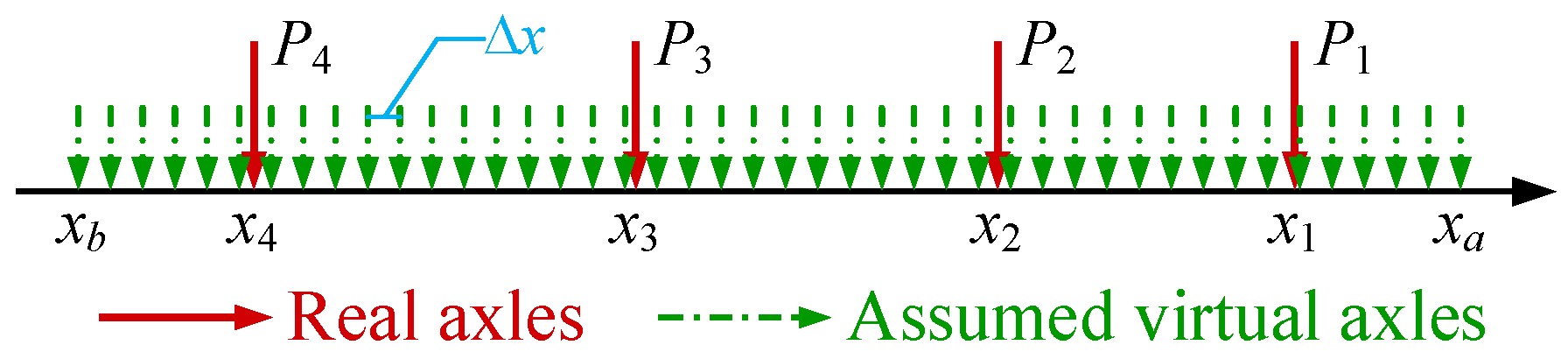
2.3. Virtual Axle Theory (Step V)

In the procedure of axle weight identification, if the vehicle has densely spaced virtual axles (VAs) and the assumed virtual axle spacing is fed into the axle weight estimating procedure, then it is natural to expect that only the identified weight of those VAs relating to real axles should be positive.

For example, Figure 2 shows a vehicle that has 4 real axles located at x₁, x₂, x₃, and x₄, with axle weights P₁, P₂, P₃, and P₄, respectively, in which the axle weights and axle locations are not known yet. Let’s assume the vehicle has a series of virtual axles evenly spaced between x_a and x_b, with an interval of Δx (x_a and x_b are intentionally set large enough to cover the wheelbase of the vehicle). Then, we can obtain weights $\tilde{P}$ of these virtual axles by using the classical Moses’ algorithm with the axle locations $\left\{x_b,x_b+\Delta x,x_b+2\Delta x,\dots ,x_a\right\}$ as the necessary information. Apparently, only the weight value of those virtual axles close to the four real axles should be positive and the others should be zeros.

However, it was found in previous work [25] that Moses’ algorithm will usually fail in this situation due to numerical instability. To address this issue, Moses’ algorithm is extended with an additional restriction based on the fact that the weight of vehicle’s axles will not be negative. Namely, the mission of finding out the correct estimation of the weight of the virtual axles turns out to be finding the solution for the following problem:

$$\mathrm{Minimize}E(P)={\Vert {S-S}^{\prime }\Vert }_2^2={\displaystyle \sum _{k=1}^K{\left(S(t_k)-S^{\prime }(t_k)\right)}^2,\mathrm{subject}\mathrm{to}P\ge 0}$$

(4)

The optimization problem in Equation (4) is a non-negative least square (NNLS) problem and can be solved by using the active set algorithm [28].

For demonstration, Figure 3 shows bending moments of a 16 m beam bridge at mid-span due to each axle weight and the gross weight of a 4-axle vehicle. The bridge is continuously supported (both ends of the bridge are fixed). The four axles are located at 0 m, 3 m, 9 m, and 12 m related to the first axle with weights of P₁ = 100 kN, P₂ = 150 kN, P₃ = 150 kN, and P₄ = 150 kN, respectively. In this case, the vehicle is assumed to have virtual axles evenly spaced within −13 m to 1 m at an interval of 0.2 m (14 m/0.2 m + 1 = 71 VAs in total). Figure 4a plots the result of step V (identified weights of the virtual axles by using the non-negative axle-weighing algorithm mentioned above). It should be noted that to be more realistic, the bridge response was polluted with 5% white Gaussian noise before being used for axle-weighing and axle-identifying purposes.

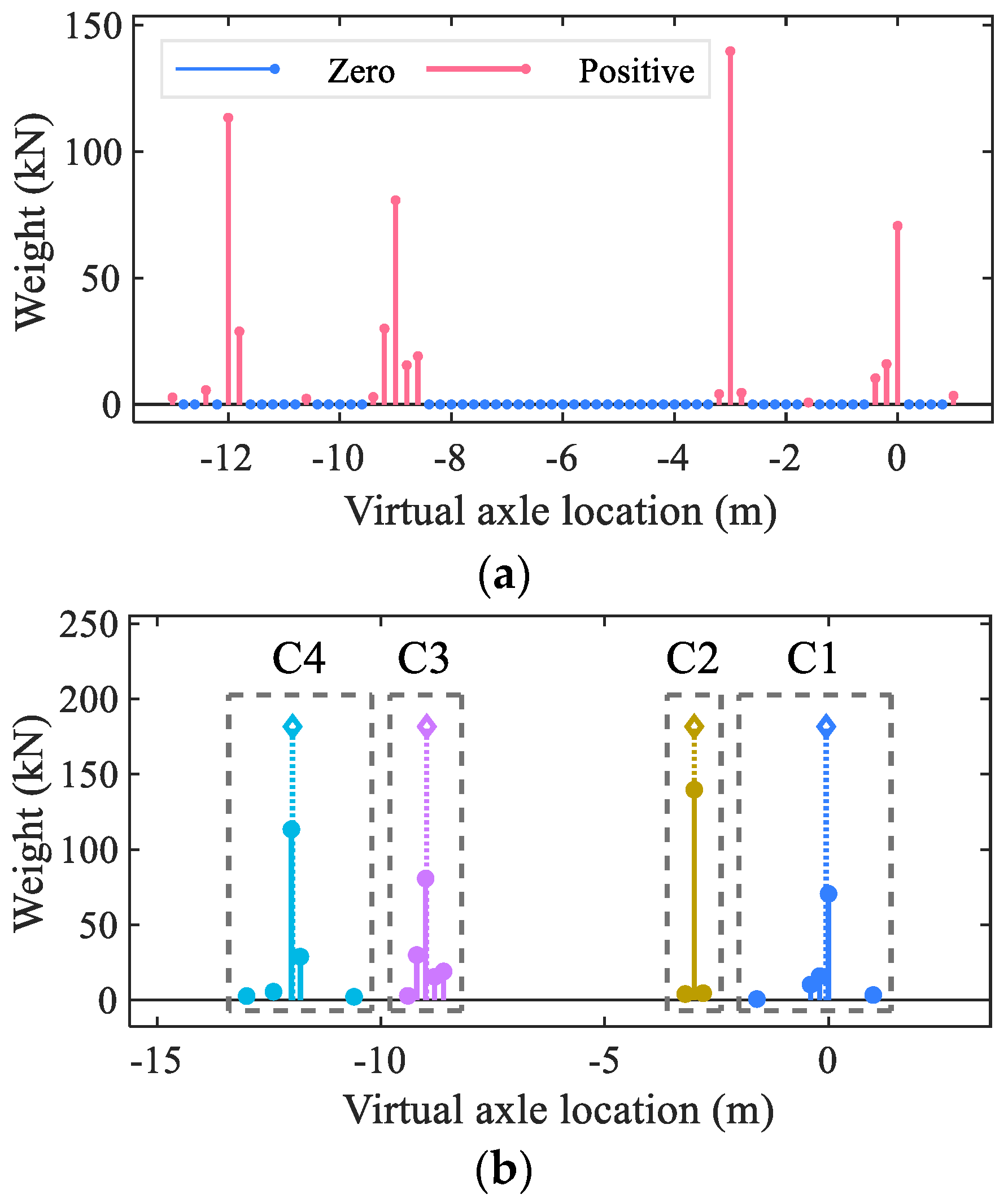
2.4. Virtual Axles Clustering (Step C)

From Figure 4a, it is seen that the four peaks of weights that are relative to the real axles are identifiable even though the actual axle location and weight are not yet achieved. Hence, the number of real axles and proper initial axle locations may be automatically obtained by clustering the positive virtual axles into categories.

The k-means method [29] is a widely used clustering method that uses the Euclidean distance to quantify the internal disparity of the cluster and was adopted as the potential clustering method. The main procedure of the clustering algorithm can be referred to in [29]. However, when using this method to divide the virtual axles into separate sets, the light virtual axles, as shown in Figure 4a, may significantly deviate the centroid of the cluster from the real axle location. To enhance the robustness of the clustering algorithm, two modifications were applied to the original k-means method such that the non-zero virtual axles could be clustered into correct sets.

First, the Euclidean distance adopted by the k-means algorithm is replaced by the following force moment-based distance function:

$$d_x(i)=\left|(x_i-x)\cdot P_i\right|$$

(5)

where d_x(i) indicates the distance from the i-th virtual axle to a certain location x.

Second, the location of the center of a cluster is defined as the point of resultant:

$$X_k={\displaystyle \sum _{j=1}^{N_k}{\widehat{x}}_j\cdot {\widehat{P}}_j}/{\displaystyle \sum _{j=1}^{N_k}{\widehat{P}}_j}$$

(6)

where N_k is the number of virtual axles of the cluster and ${\widehat{x}}_j$ and ${\widehat{P}}_j$ are the locations and weights, respectively, of the j-th virtual axle of the cluster.

It should be noted that the best number K of the cluster centroids is determined using the elbow method [27] with the elbow criterion (the between-group variance to the total variance) configured to be 90% [30]. In a real application, it might be useful to recheck and choose a proper elbow criterion for the specific bridge and traffic situation. Moreover, the k-mean++ seeds initialization technique [31] is used to improve the convergence speed and the quality of the final solution, and the clustering procedure is performed multiple times to avoid poor clustering results.

By using this clustering method, the axle count and axle locations of the vehicle can be obtained and then can be fed into Equation (2). Then an initial estimate of axle weights can be obtained by solving Equation (3) or Equation (4).

2.5. Gradient Method (Step G)

In numerical simulation and laboratory tests, it was found that the identified axle weights may not be the best estimation. The reason for this is mainly because the quality of the identified axle locations from Section 2.4 is not good enough.

To simultaneously obtain the best axle location and weight estimation, an iterative method was proposed. In this method, the objective function is defined as

$$U(x)=\underset{\_}{E}(x)$$

(7)

where $\underset{\_}{E}(x)$ is the minimum value of the error function E(x) of Equation (4) relative to axle locations x. The axle locations then can be obtained by finding out the global minimum of U. To solve this optimization problem, the following iterative scheme based on the gradient method is proposed:

$$\begin{array}{c}\lambda (x^j)=\nabla U=\frac{U(x^j+h^j)-U(x^j)}{h^j}\\ x^{j+1}=x^j-\mathrm{sign}(\lambda (x^j))\cdot h^j\end{array}$$

(8)

where $\lambda$ is the gradient of U, j indicates the sequence number of the iteration, and $h={\{h_1,h_2,\dots ,h_i,\dots \}}^T$ is the step size for the iterations, which also serves as the vector of axle location increments for calculating the gradient at position x. The element $h_i$ of h is initially set to be the same as the specified virtual axle spacing Δx and is reduced by half if the sign of gradient changes during iterations:

$$h_i^{j+1}=\{\begin{array}{cc}\begin{array}{l}{h}_i^j\\ h_i^j/2\end{array}& \begin{array}{l}\mathrm{sign}\left(\lambda (x_i^{j+1})\right)=\mathrm{sign}\left(\lambda (x_i^j)\right)\\ \mathrm{sign}\left(\lambda (x_i^{j+1})\right)\ne \mathrm{sign}\left(\lambda (x_i^j)\right)\end{array}\end{array}$$

(9)

The axle location result of the clustering section is taken as the initial value $x^0$ for the iteration method defined by Equation (8). The procedure is then repeated until the objective function U converges to its minimum. At this point, the corresponding x is taken as the best estimation of the real axle location by the proposed VCG method. Besides, the best prediction of the axle weights P is also determined when the iteration process is finished.

For the previously demonstrated example, C1~C4 in Figure 4b show the centroid of the four clusters calculated via Equation (6). These values are taken as an initial assumption of real axle locations for the optimization method stated in Equation (8). The iteration process is then repeated until convergence. Figure 4c shows the value of the objective function U relative to the iteration times. The axle weights and axle spacings were finally identified as 100.4 kN, 149.1 kN, 148.1 kN, and 152.6 kN and 2.95 m, 5.98 m, and 3.00 m, respectively. Figure 4d shows the source moment (to be realistic, the true moment was polluted by 5% Gaussian error) and the moment rebuilt using identified axle locations and weights. From this figure, it can be seen that the rebuilt moment matches the source moment well. It should be marked that it only takes about 25 iterations to reach convergence, not only for this example, but also for the majority of the numerical and laboratory experiments in the later sections. Namely, the proposed method has a higher efficiency than the previously proposed VA method, which solves Equation (3) for dozens to millions of combinations of potential axle locations (for details of the VA method, please refer to [26]).

3. Numerical Study

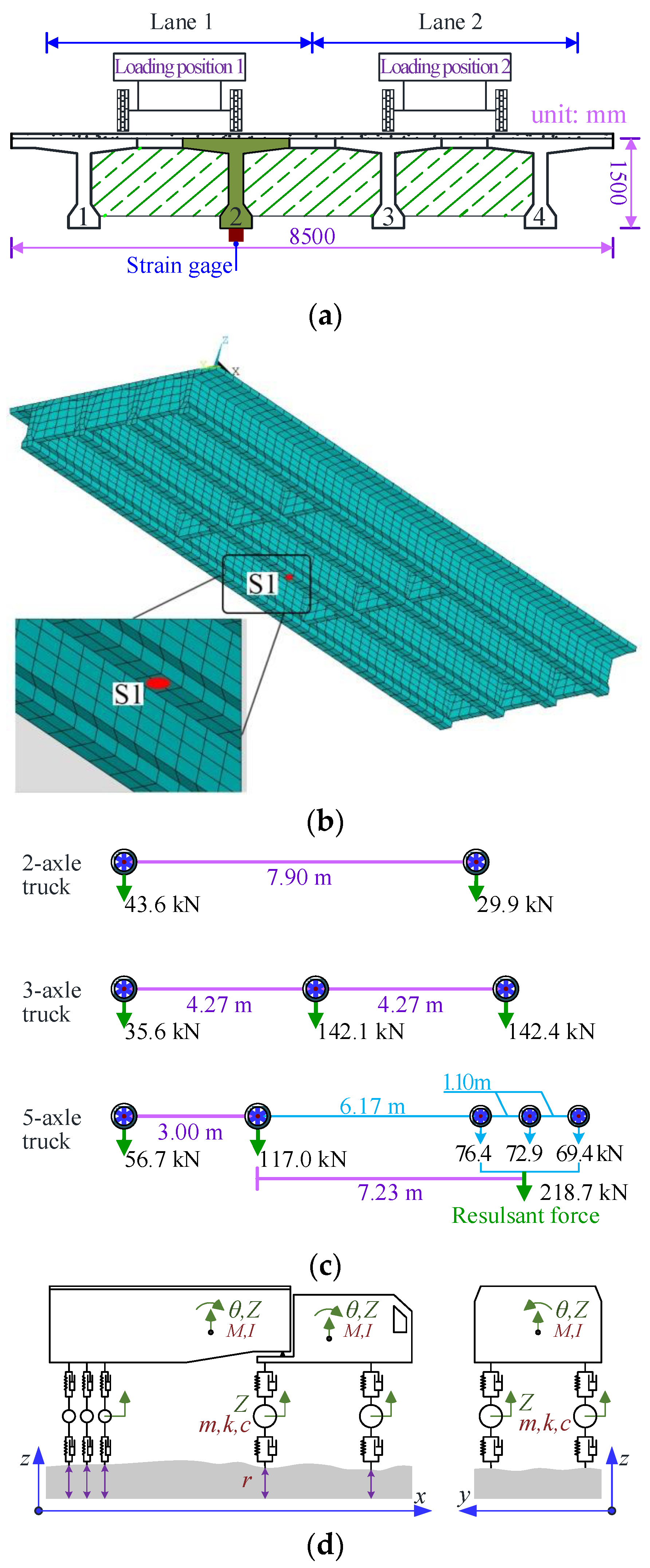
3.1. Vehicle–Bridge Coupled Vibration System

The motion of the vehicle–bridge interactive (VBI) vibration can be expressed as the following equations [32] (Deng and Cai 2010):

$$\{\begin{array}{cc}\begin{array}{l}{\mathit{M}}_{\mathrm{V}}\ddot{Z}+{\mathit{C}}_{\mathrm{V}}\dot{Z}+{\mathit{K}}_{\mathrm{V}}Z={\mathit{N}}_{\mathrm{V}}\cdot F_c+G_{\mathrm{V}}\\ {\mathit{M}}_{\mathrm{B}}\ddot{Y}+{\mathit{C}}_{\mathrm{B}}\dot{Y}+{\mathit{K}}_{\mathrm{B}}Y={\mathit{N}}_{\mathrm{B}}\cdot F_c\end{array}& \end{array}$$

(10)

where ${\mathit{M}}_{\mathrm{V}}$,${\mathit{C}}_{\mathrm{V}}$,${\mathit{K}}_{\mathrm{V}}$, N_V and ${\mathit{M}}_{\mathrm{B}}$,${\mathit{C}}_{\mathrm{B}}$,${\mathit{K}}_{\mathrm{B}}$,${\mathit{N}}_{\mathrm{B}}$ are the mass, damping, stiffness matrices, and shape functions of the vehicle and the bridge, respectively; Z and Y are the motions in the directions of the degrees of freedom of the vehicle and the bridge, respectively; $F_c={\left\{f_1,f_2,\dots ,f_{2N_{\mathrm{A}}}\right\}}^T$ is the vector of the contact forces between the vehicle tires and the bridge deck surface due to the difference of vehicle tire motion, bridge motion, and bridge surface roughness in the vertical direction at the contact points; and $G_{\mathrm{V}}$ is the vector of the vertical forces acting on the center of the masses of the vehicle due to gravity. A numerical routine based on the modal superposition method and the iterative Newmark-β algorithm was developed to solve Equation (10) [23,32]. The derivation of the dynamic Equation (10) and the detailed procedure of the numerical solution can be referred to in [33,34]. After the equation was solved, the displacement response of the bridge was then used to calculate the strain response of the bridge according to the strain–displacement relationship. In this study, the flexural strain of the bridge was used for axle weight and spacing identification. It should be noted that any type of bridge response sensitive to the longitudinal loading position of axle load should be compatible with the VCG method.

3.2. Simulation Setup

A 20 m simply supported RC bridge and three vehicle models (2-axle, 3-axle, and 5-axle) were used for the numerical verification. Young’s modulus and the density of the bridge material were 34.5 GPa and 2653 kg/m³, respectively. The bridge section and lateral loading position are shown in Figure 5a; the FE model and sensor station are shown in Figure 5b. More details about the bridge FE model can be referred to in [23]. The load configurations of the trucks are illustrated in Figure 5c. The gross vehicle weight (GVW) of the trucks was 73.5 kN, 320.1 kN, and 392.4 kN, respectively. Figure 5d shows the analytic model of the 5-axle truck for illustration purpose. Detailed parameters of the dynamic truck models can be found in [23,26]. During the test, trucks were set to run at five velocities: 10 m/s, 15 m/s, 20 m/s, 25 m/s, and 30 m/s. Smooth and coarse bridge deck surfaces were considered in the test, where the coarse scenario included two levels of the road surface condition (RSC), i.e., class A and class B according to the ISO8608 (1995) standard. For each coarse loading case, 10 random road roughness profiles were generated and the trucks were independently run 10 times under each of the roughness profiles. Then, the strains measured from the second girder at mid-span were used for identification, and the statistic of the values of the identified results was used for statistical analysis later.

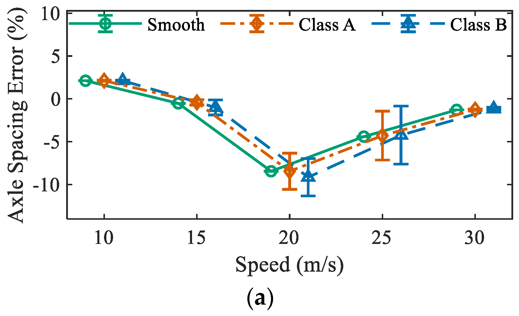
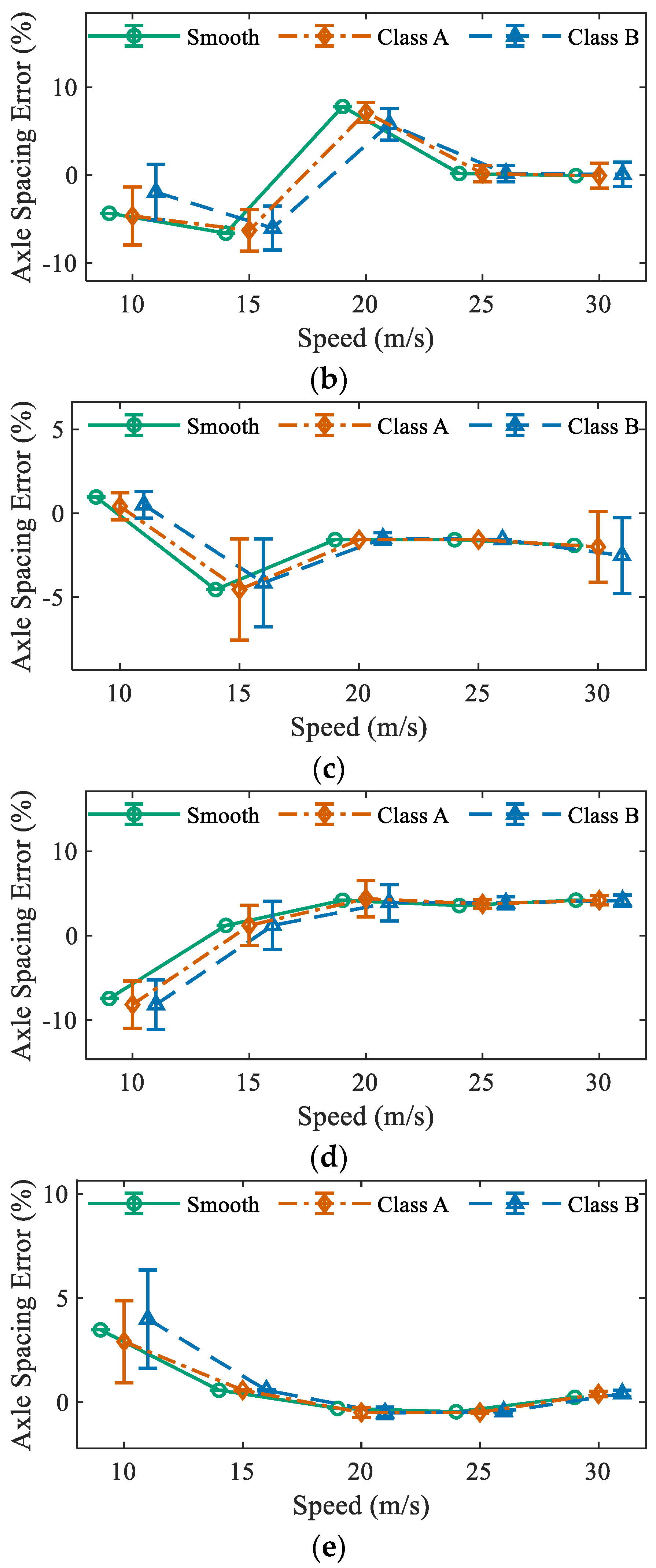
3.3. Results and Discussion

By solving Equation (10), the displacement of the bridge FE model was obtained. The longitudinal strain (normal strain) of the second girder at mid-span was then calculated based on the strain–displacement relationship of FE method theory. Figure 6a shows the influence line of the strain response of the second girder for both loading positions. Figure 6b shows typical strains of the bridge under moving vehicle loads.

Figure 7, Figure 8 and Figure 9 show stack bar plots of identified axle weights for the 2-axle truck, 3-axle truck, and 5-axle truck. For each truck, according to the test plan, there were 210 simulation tests (2 lateral loading position × 5 velocities × 2 RSC level × 10 runs + 2 lateral loading position × 5 velocities × 1 smooth RSC × 1 run). From these figures, it is first seen that the identification results of the gross weight were all stable and close to the true gross weight (the accumulation of the AW stacks is gross weight). Second, the identified axle weights for the 2-axle truck and the 3-axle truck as well as the first two axles of the 5-axle truck under most simulation cases were close to the true values (real weight of the axles). Third, the identified axle weights for the last three axles of the 5-axle truck might have largely deviated from their true values. This is because the last three axles of the 5-axle truck are closely spaced (1.1 m). Fortunately, the sum of the identified weights of the three axles was stable and close to the true weight (real value) of the three tandem axles. Thus, in the following sections, the last three axles were treated as a single group in the error analysis as was done by many researchers [11,35].

It should also be marked that all the results for the two loading positions (centers of the left lane and the right lane) were identified using the proposed method based on the strain responses measured from the same second girder. It can be concluded that the lateral loading position of the moving vehicles does not show a noticeable influence on the proposed method.

Figure 10 plots the relative error of identified axle weights for the three axles (or axle group) of the 5-axle truck. Figure 11 plots the relative error of the identified gross weights for the three trucks. The error bars shown in the figure indicate 90% confidence intervals. It can be seen that the mean values of identification errors under a bad RSC were not always larger than those under a good RSC, while the 90% confidence intervals of errors generally increased as the road surface became worse Vehicle speed did not show any certain pattern for the three axles (axle group). Besides, it seems that the lighter the axle weight is, the larger the identified errors will be. However, under all considered cases, the mean values of identified error for all the axles were all within 5% and those for gross vehicle weights were all within 3%. This indicates that the proposed method has the ability to identify axle and gross weights of a vehicle with high accuracy under different speeds and coarse road surface conditions.

Figure 12 shows the identification error of axle spacing for the three trucks. For the 5-axle truck, the last three axles were treated as a single axle (group), and AS2 represents the distance between the second axle to the center of the resultant force of the three axles. Road surface conditions showed the same effect on the identified spacing errors. Vehicle speed did not show any certain pattern again. In general, the mean values of the spacing errors were under 10%, which is still favorable, though they were larger than those of axle weights.

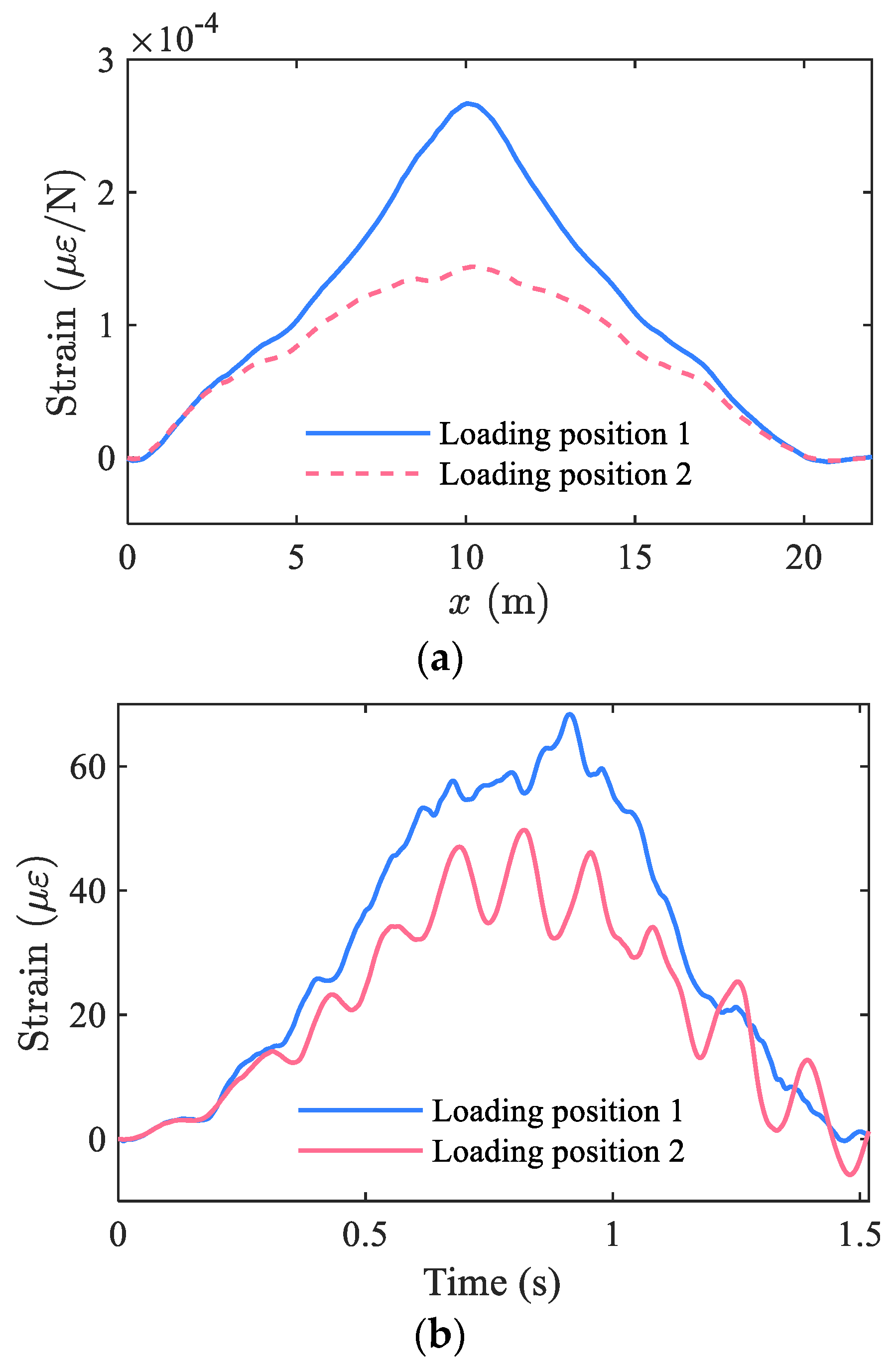
4. Experiment Validation

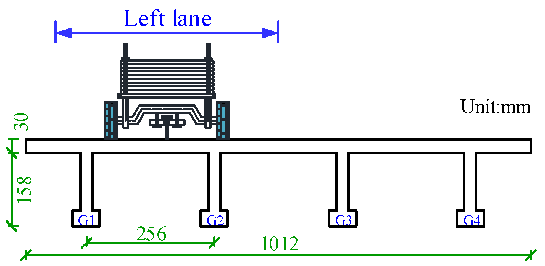
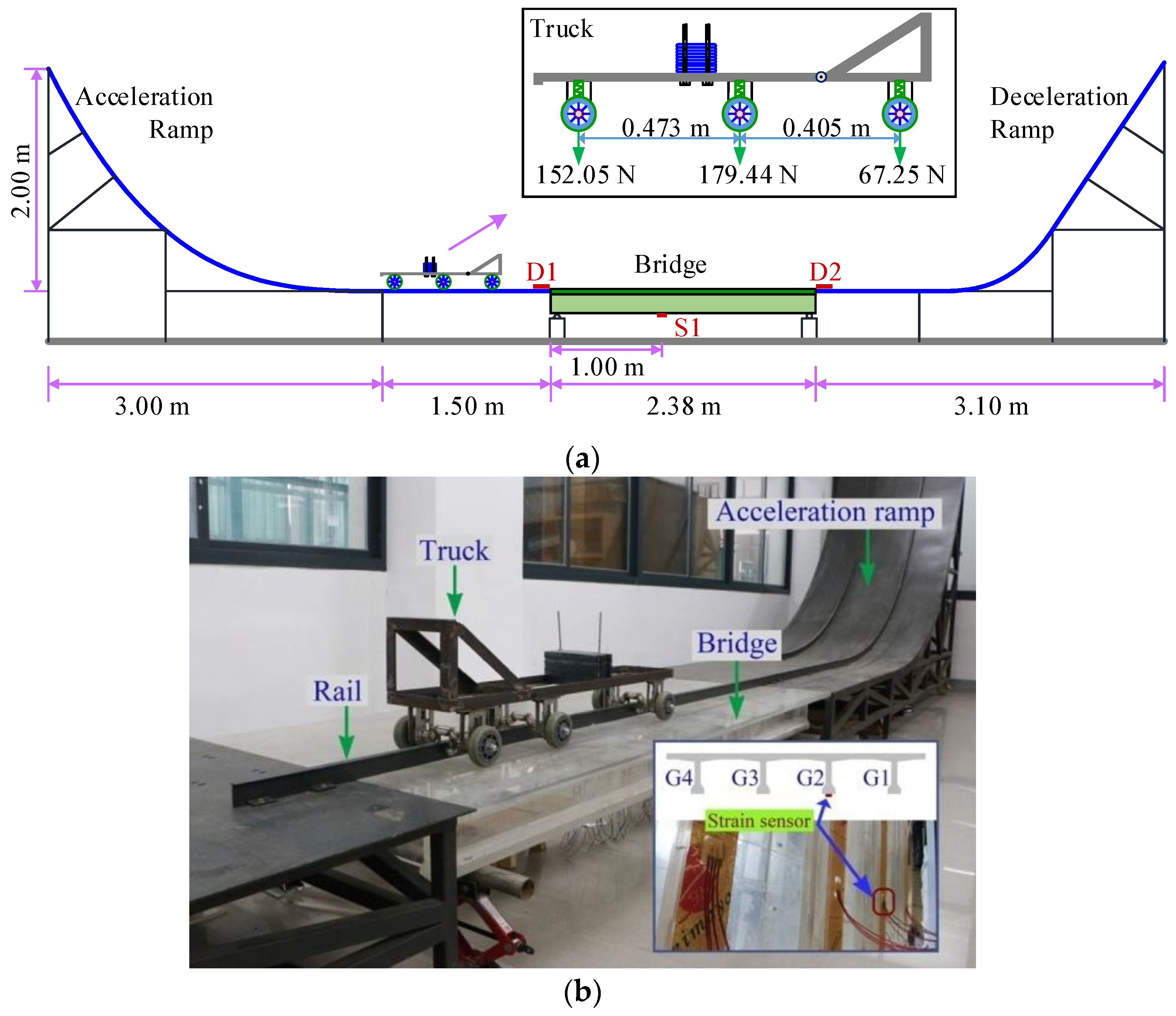
4.1. Test Setup

To verify the proposed method, experiments on a scaled model test in the laboratory were conducted. Figure 13a shows the test platform consisting of an accelerating ramp, a test bridge model, and a decelerating ramp. Figure 13b shows a photo of the test platform. The span length and width of the prototype bridge were 20 m and 8.5 m, respectively. The bridge model was made of polymethyl methacrylate (PMMA) based on the similarity principle with a scale ratio of 1:8.403. Figure 14 shows the cross section of the scaled bridge model. The bridge was simply supported by piles 5 cm away from both ends. The scaled truck model adopted in the tests was mainly made of steel with the same scale ratio, as shown in Figure 13. The prototype truck was a 3-axle truck with 348 kN gross weight and 7.38 m wheelbase (3.6 m for the first axle spacing and 4.2 m for the last axle spacing). The details of the bridge and truck model can be found in [23].

A foil strain gauge was attached to the bridge under the second girder at the S1 section, as shown in Figure 13a. Two foil strain gauges were placed on the top of the road before and after the bridge, marked as D1 and D2, respectively, in Figure 13 to serve as speed and axle spacing detectors. The bridge strain measured using the sensor at station S1 was then used as input to the proposed identification method. The strains measured using D1 and D2 sensors were used to determine the vehicle speed, which was also used as the input speed for the proposed method.

During the tests, the vehicle was lifted to a certain position on the acceleration ramp and released to gain the desired speed to pass over the test bridge, and then was slowed down on the deceleration ramp due to gravity. The lateral loading position of the truck was controlled by a rail fixed on the traveling road, as shown in Figure 14. By adjusting the height of the position on the acceleration ramp the truck was hauled to, tests with vehicle speeds from 1 m/s to 5 m/s were performed, which corresponds to a range of 10.4 km/h to 52.2 km/h for full-scale tests according to the similarity principle.

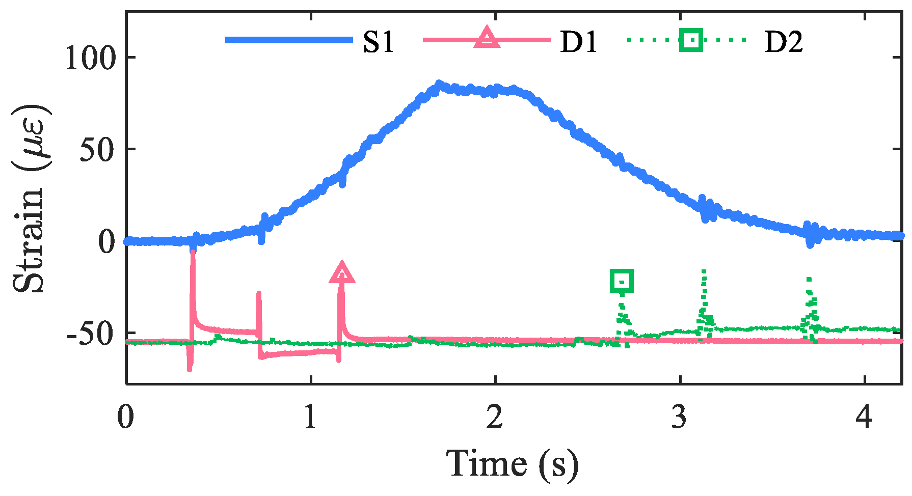
4.2. Results and Discussion

Figure 15 plots the typical time histories of strains measured from sensors S1, D1, and D2. It is seen that sharp peaks occurred on the D1 and D2 signals. By identifying those peaks, the vehicle speed and axle spacing were obtained. The detected vehicle speed and the time histories of strain S1 were fed into the proposed method to identify axle spacing and weights. In the laboratory tests, the truck was set to run five times for each of the desired speeds 1 m/s, 2 m/s, 3 m/s, 4 m/s, and 5 m/s. Figure 16 shows the true and identified weights and axle spacing of the truck for the 25 test runs. It can be seen from Figure 16 that the axle weight and axle spacing can be successfully identified from the bridge strain by using the proposed method.

To check the accuracy of the proposed VCG method, the relative errors of the identified result were calculated and are listed in

Table 1. Identified weight errors using the VCG method.

Average Speed (m/s)	Relative Error (%)
	AW1		AW2		AW3		GVW
	u	w	u	w	u	w	u	w
1.02	2.0	1.5	−2.9	0.8	2.3	1.0	−0.1	0.2
2.05	6.1	2.3	−2.9	1.3	−0.2	1.0	−0.3	0.2
3.02	9.2	7.6	−4.1	2.4	−4.1	3.4	−1.8	1.5
4.03	3.0	3.6	−1.7	1.6	−0.5	1.8	−0.4	0.5
5.03	−2.6	2.9	0.4	1.8	−1.6	2.3	−0.9	0.9

,

Table 2. Identified weight errors using Moses’ algorithm.

Average Speed (m/s)	Relative Error (%)
	AW1		AW2		AW3		GVW
	u	w	u	w	u	w	u	w
1.02	−3.7	1.0	6.6	1.7	−5.4	2.0	0.3	0.2
2.05	0.7	2.0	−0.4	1.2	−0.1	1.0	−0.1	0.2
3.02	−2.7	3.8	1.1	1.5	−0.6	1.1	−0.2	0.8
4.03	5.5	4.7	−2.5	3.1	0.8	3.3	0.1	0.7
5.03	−9.7	2.1	3.1	2.5	−1.8	1.8	−0.9	1.3

,

Table 3. Identified spacing errors using the VCG method.

Average Speed (m/s)	Relative Error (%)
	AS1		AS2
	u	w	u	w
1.02	1.9	1.3	−3.8	1.0
2.05	2.5	2.0	−4.1	1.2
3.02	−1.5	3.5	−4.9	1.7
4.03	2.7	1.7	−3.1	1.8
5.03	−0.0	2.4	−2.4	1.4

and

Table 4. Identified spacing errors using the axle detector.

Average Speed (m/s)	Relative Error (%)
	AS1		AS2
	u	w	u	w
1.02	−0.9	0.1	7.6	0.4
2.05	−1.7	0.1	2.7	0.4
3.02	−0.8	0.4	0.1	0.2
4.03	2.4	0.4	−1.5	0.4
5.03	−4.0	1.4	−0.6	0.6

. In these tables, u and w denote the average value and the 90% confidence interval of the relative error of the five runs for each speed, respectively. Table 1 and Table 3 show the relative errors of weight and spacing based on the proposed VCG method, respectively; Table 2 shows the relative weight error of Moses’ algorithm; and Table 4 shows the relative error of axle spacing directly identified from D1 and D2 signal. It should be noted that the vehicle axle spacings are required to be preliminary detected from the D1 and D2 sensors for Moses’ algorithm but not for the proposed VCG method.

From Table 1 and Table 2, it can be seen that both methods obtained axle weights with accuracy. In most tests, the weight errors of the VCG method were smaller than 5%, while only for the lightest axle AW1, two errors exceeded 5% and one of them reached 9.2%. For Moses’ algorithm, most errors were also below 5%, and there were three scenarios with weight errors over 5% and one of them reached 9.7%. The relative errors of gross vehicle weight (GVW) are also listed in the tables. It shows that Moses’ algorithm has better performance on gross weight identification than the VCG method. However, all these errors were within 2%, indicating that high accuracy is achieved on the gross weight identification by both methods. In summary, the proposed VCG method is as accurate as Moses’ algorithm on gross weight identification and shows better performance on axle weight identification.

Table 3 presents the relative errors of axle spacing identified using the proposed VCG method. These relative errors were all below 5%, implying that the axle spacing identified using the VCG method is reliable. By comparing with the identification errors directly using the axle-detecting sensors D1 and D2, it was found that the maximum of average relative errors of the VCG method was smaller than that of directly detected results, while the maximum 90% confidence interval of the relative errors from the directly detected result was narrower than that of the VCG method. It implies that the VCG method has a close or even higher accuracy than the dedicated axle detectors on axle-spacing identification, though the results may not be as stable as the directly detected results.

5. Conclusions

Detecting the axle spacing, axle weight, and gross weight of passing vehicles is vital for traffic monitoring on highway bridges. A new approach named the VCG method is proposed in this paper to fulfill this need. Different from the conventional Moses’ algorithm or its derivates that require axle spacing information to be primarily determined using an external device before the weight identification procedure, this method can simultaneously obtain the axle spacing and weight directly from the global strain response of the bridge. Thus, it serves as a promising alternative for the nothing-on-road (NOR) BWIM system.

In the study, comprehensive numerical experiments and scaled model tests were performed to validate the proposed approach. The performance of the proposed method was evaluated considering different vehicle velocities, road surface roughness, lateral loading positions, and truck models. Detailed conclusions are listed below:

(1)

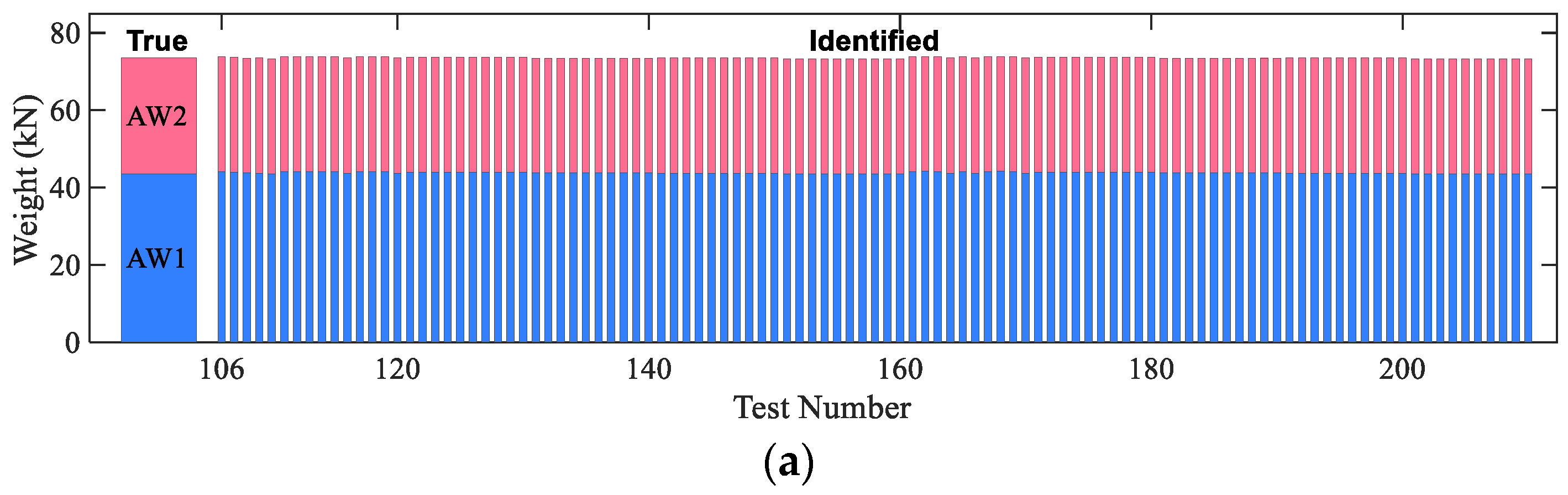
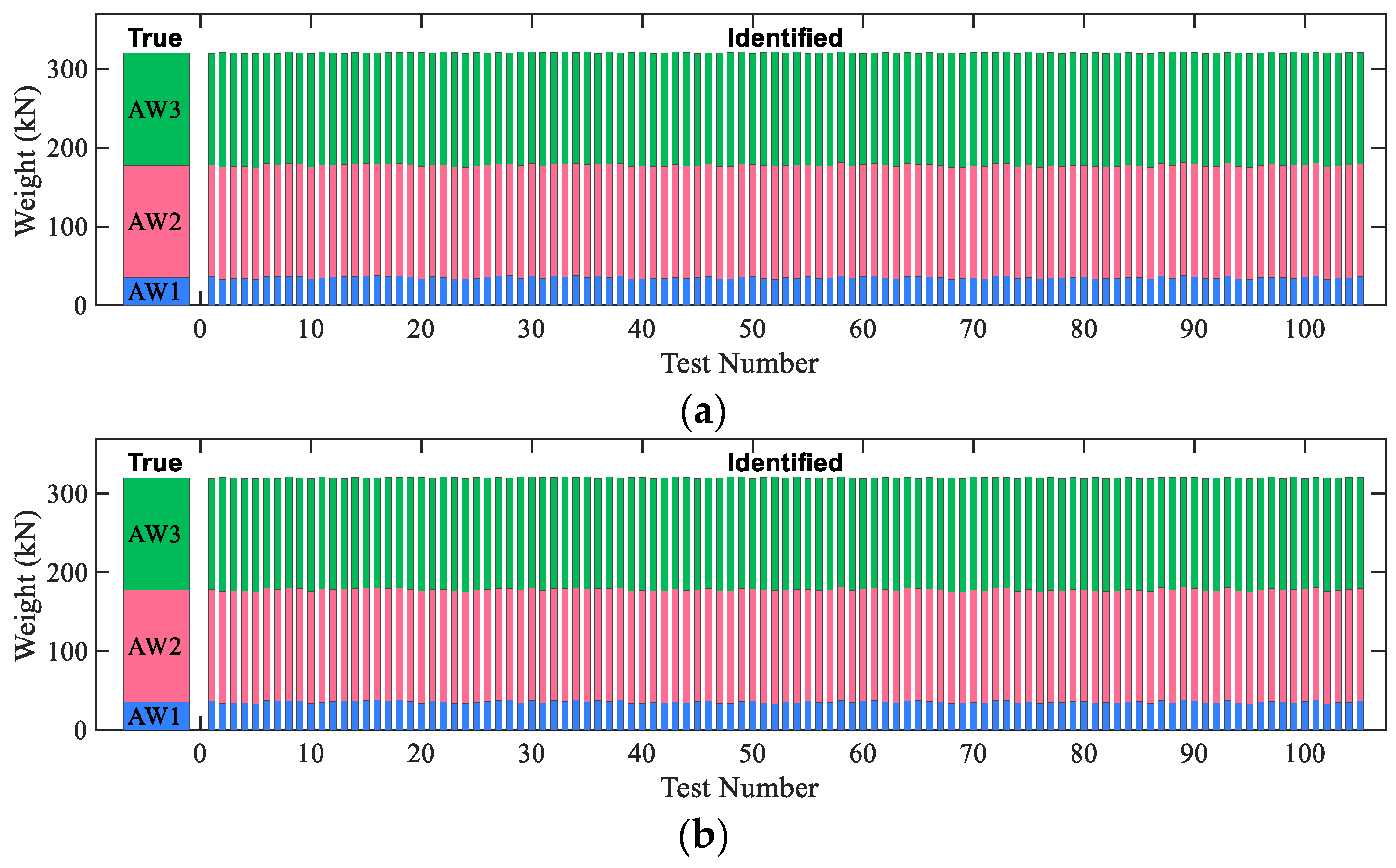
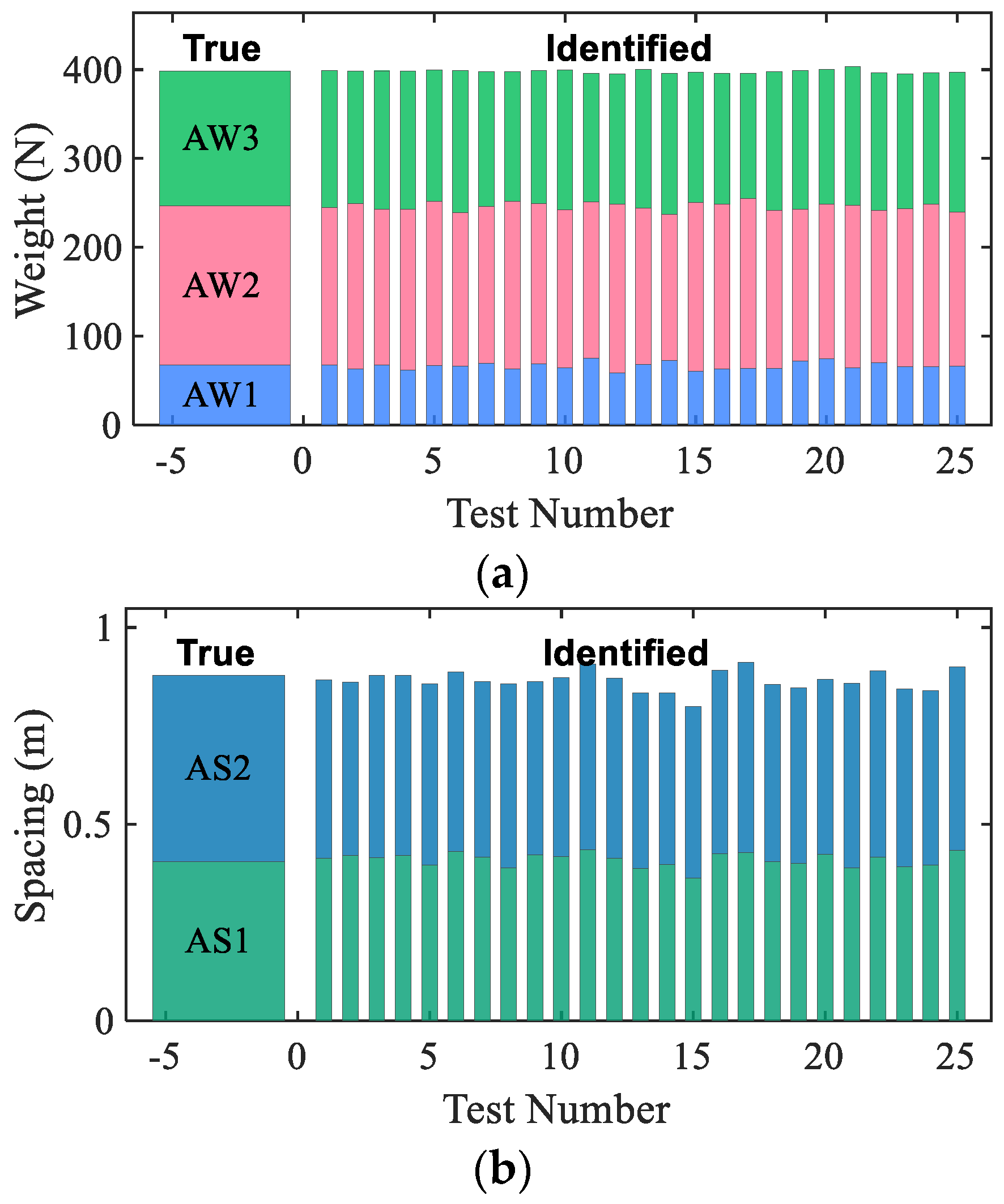
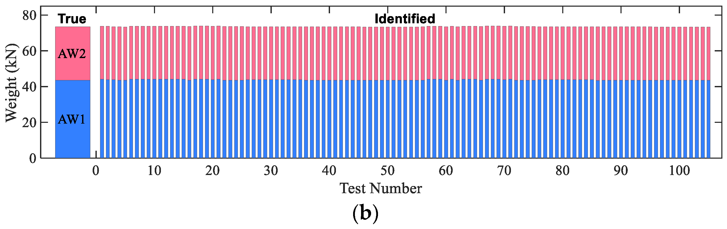
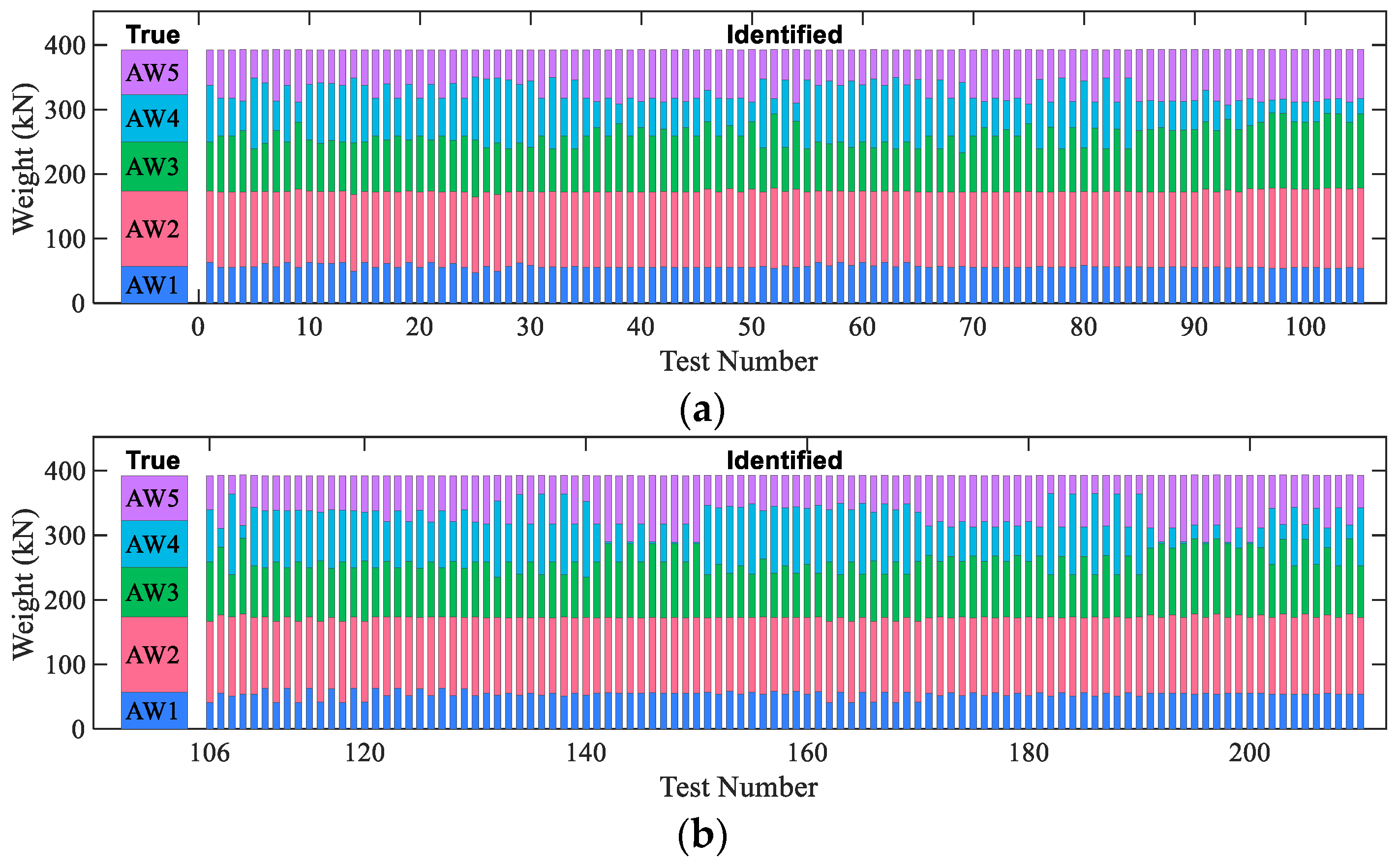
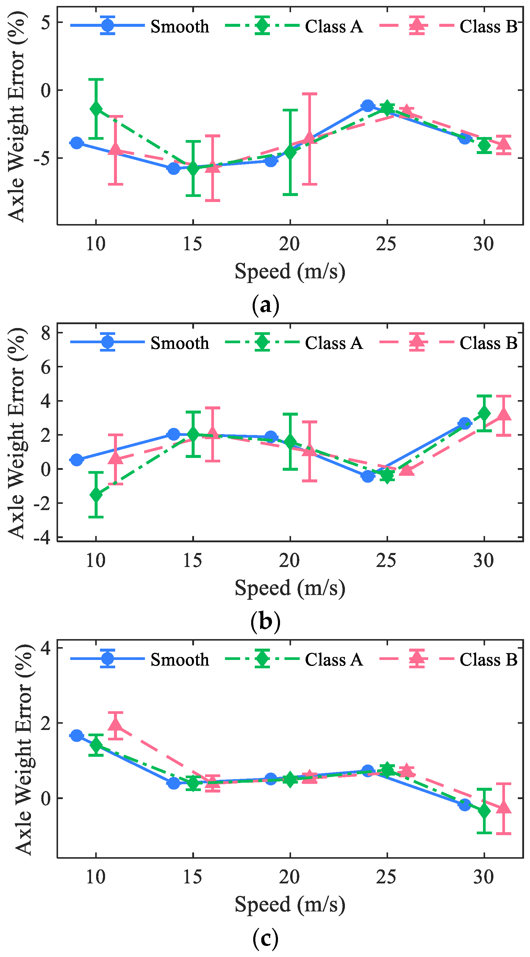
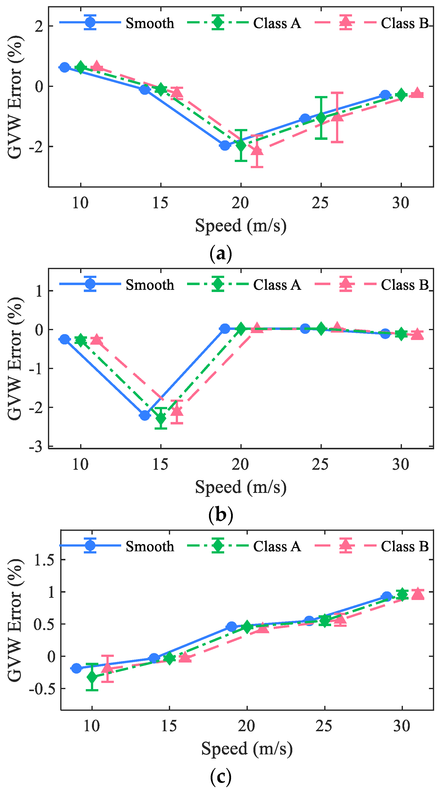
The weight of vehicle axles was correctly detected by the VCG method based on the bridge strain response and vehicle speed. The VCG method has similar accuracy as Moses’ algorithm on gross weight identification but has better accuracy than on axle weight identification.

(2)

The VCG method can also identify the location of vehicle axles. The identification accuracy was comparable to the direct method (using a pressure-sensitive sensor placed on the top surface of the road) but without the need for installing a dedicated axle detector.

(3)

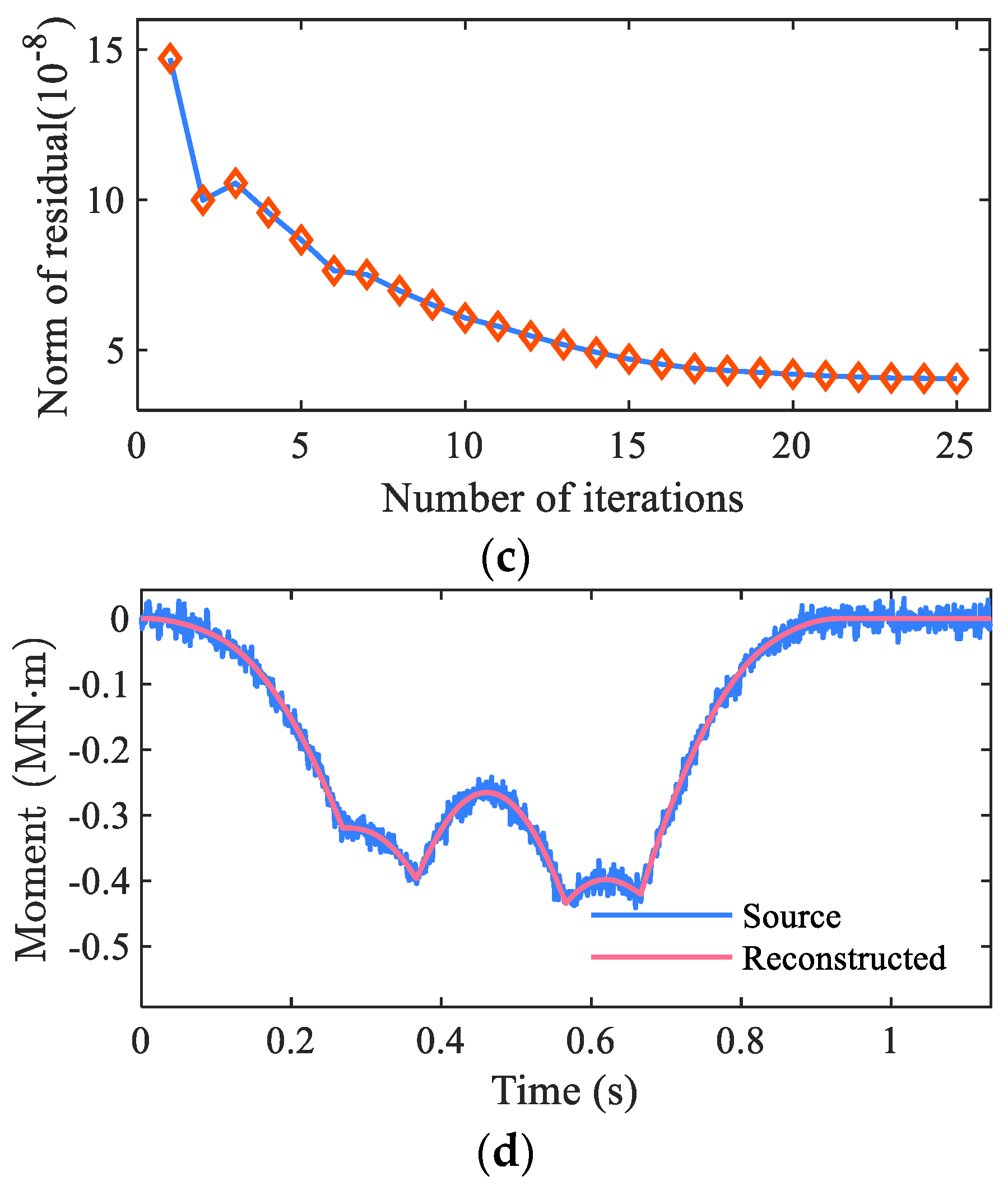
The proposed method generally converges within dozens of iterations. The computation efficiency proves that it is suitable for real-time application.

It should also be noted that the proposed method theoretically works for any type of bridge or bridge response as long as the response of the bridge is sensitive to the longitudinal position of axle load, since it sets no restrictions on the bridge type or response type. Moreover, these findings were concluded from single-truck passing scenarios via numerical and laboratory tests. The performance of the proposed method should be further investigated in future studies through field tests and considering the multiple presence of trucks on a bridge.

References

1. Deng, L.; Bi, T.; He, W.; Wang, W. Vehicle weight limit analysis method for reinforced concrete bridges based on fatigue life. China J. Highw. Transp. 2017, 30, 72–78. [Google Scholar]
2. Deng, L.; Duan, L.L.; He, W.; Ji, W. Study on vehicle model for vehicle-bridge coupling vibration of highway bridges in China. China J. Highw. Transp. 2018, 317, 92–100. [Google Scholar]
3. Jacob, B.; Feypell-de La Beaumelle, V. Improving truck safety: Potential of weigh-in-motion technology. IATSS Res. 2010, 34, 9–15. [Google Scholar] [CrossRef] [Green Version]
4. Richardson, J.; Jones, S.; Brown, A.; O’Brien, E.J.; Hajializadeh, D. On the use of bridge weigh-in-motion for overweight truck enforcement. Int. J. Heavy Veh. Syst. 2014, 21, 83–104. [Google Scholar] [CrossRef]
5. Moses, F. Weigh-in-motion system using instrumented bridges. Transp. Eng. J. 1979, 105, 233–249. [Google Scholar] [CrossRef]
6. Quilligan, M.; Karoumi, R.; O’Brien, E.J. Development and testing of a 2-dimensional multi-vehicle bridge-wim algorithm. In Proceedings of the 3rd International Conference on Weigh-in-Motion (ICWIM3), Orlando, FL, USA, 13–15 May 2002; Wiley: New York, NY, USA, 2002. [Google Scholar]
7. Zhao, H.; Uddin, N.; O’Brien, E.J.; Shao, X.; Zhu, P. Identification of vehicular axle weights with a bridge weigh-in-motion system considering transverse distribution of wheel loads. J. Bridge Eng. 2014, 19, 165–184. [Google Scholar] [CrossRef] [Green Version]
8. Yu, Y.; Cai, C.; Deng, L. State-of-the-art review on bridge weigh-in-motion technology. Adv. Struct. Eng. 2016, 19, 1514–1530. [Google Scholar] [CrossRef]
9. Lydon, M.; Taylor, S.E.; Robinson, D.; Mufti, A.; Brien, E.J.O. Recent developments in bridge weigh in motion (B-WIM). J. Civ. Struct. Health Monit. 2015, 6, 69–81. [Google Scholar] [CrossRef] [Green Version]
10. Ji, S.; Wang, R.; Shu, M.; Han, W.; Lan, X.; Wang, X.; Yin, W.; Cheng, Y. Improvement of vehicle axle load test method based on portable WIM. Meas. 2021, 173, 108626. [Google Scholar] [CrossRef]
11. Jacob, B. Weighing-in-Motion of Axles and Vehicles for Europe (WAVE). Rep. of Work Package 1.2; Laboratoire Central des Ponts et Chaussées: Paris, France, 2001. [Google Scholar]
12. Ieng, S.S.; Zermane, A.; Schmidt, F.; Jacob, B. Analysis of B-WIM signals acquired in Millau orthotropic viaduct using statistical classification. In Proceedings of the International Conference on Weigh-in-Motion (ICWIM 6), Dallas, TX, USA, 4–7 June 2012; Wiley: New York, NY, USA, 2012; pp. 43–52. [Google Scholar]
13. Kalin, J.; Žnidarič, A.; Lavrič, I. Practical implementation of nothing-on-the-road bridge weigh-in-motion system. In Proceedings of the International Symposium on Heavy Vehicle Weights and Dimensions, State College, PA, USA, 18–22 June 2006; Pennsylvania State University: State College, PA, USA, 2006. [Google Scholar]
14. Wall, C.J.; Christenson, R.E.; Mcdonnell, A.M.H.; Jamalipour, A. A Non-Intrusive Bridge Weigh-in-Motion System for a Single Span Steel Girder Bridge Using Only Strain Measurements; Rep. No. CT-2251-3-09-5, 9–10; Connecticut DOT: Rocky Hill, CT, USA, 2009.
15. Kalhori, H.; Alamdari, M.M.; Zhu, X.; Samali, B.; Mustapha, S.J.M.S. Non-intrusive schemes for speed and axle identification in bridge-weigh-in-motion systems. Meas. Sci. Technol. 2017, 28, 025102. [Google Scholar] [CrossRef]
16. O’Brien, E.J.; Hajializadeh, D.; Uddin, N.; Robinson, D.; Opitz, R. Strategies for axle detection in bridge weigh-in-motion systems. In Proceedings of the International Conference on Weigh-in-Motion (ICWIM 6), Dallas, TX, USA, 4–7 June 2012; Wiley: New York, NY, USA, 2012. [Google Scholar]
17. Bao, T.; Babanajad, S.K.; Taylor, T.; Ansari, F. Generalized method and monitoring technique for shear-strain-based bridge weigh-in-motion. J. Bridge Eng. 2016, 21, 04015029. [Google Scholar] [CrossRef]
18. Dunne, D.; O’Brien, E.J.; Basu, B.; Gonzalez, A. Bridge WIM systems with Nothing on the Road (NOR). In Proceedings of the Fourth International Conference on Weigh-in-Motion, Taipei, Taiwan, 20–23 February 2005. [Google Scholar]
19. Chatterjee, P.; O’Brien, E.; Li, Y.; González, A. Wavelet domain analysis for identification of vehicle axles from bridge measurements. Comput. Struct. 2006, 84, 1792–1801. [Google Scholar] [CrossRef] [Green Version]
20. Yu, Y.; Cai, C.; Deng, L. Vehicle axle identification using wavelet analysis of bridge global responses. J. Vib. Control. 2017, 23, 2830–2840. [Google Scholar] [CrossRef]
21. Ojio, T.; Carey, C.H.; O’Brien, E.J.; Doherty, C.; Taylor, S.E. Contactless Bridge Weigh-in-Motion. J. Bridge Eng. 2016, 21, 04016032. [Google Scholar] [CrossRef] [Green Version]
22. Xia, Y.; Jian, X.; Yan, B.; Su, D. Infrastructure Safety Oriented Traffic Load Monitoring Using Multi-Sensor and Single Camera for Short and Medium Span Bridges. Remote Sens. 2019, 11, 2651. [Google Scholar] [CrossRef] [Green Version]
23. He, W.; Deng, L.; Shi, H.; Cai, C.S.; Yu, Y. Novel virtual simply supported beam method for detecting the speed and axles of moving vehicles on bridges. J. Bridge Eng. 2017, 22, 04016141. [Google Scholar] [CrossRef]
24. Chen, S.Z.; Wu, G.; Feng, D.C.; Zhang, L. Development of a bridge weigh-in-motion system based on long-gauge fiber bragg grating sensors. J. Bridge Eng. 2018, 23, 18. [Google Scholar] [CrossRef]
25. Deng, L.; He, W.; Yu, Y.; Cai, C.S. Equivalent shear force method for detecting the speed and axles of moving vehicles on bridges. J. Bridge Eng. 2018, 23, 04018057. [Google Scholar] [CrossRef]
26. He, W.; Ling, T.; O’Brien, E.J.; Deng, L. Virtual axle method for bridge weigh-in-motion systems requiring no axle detector. J. Bridge Eng. 2019, 24, 04019086. [Google Scholar] [CrossRef]
27. Thorndike, R.L. Who belongs in the family? Psychometrika 1953, 18, 267–276. [Google Scholar] [CrossRef]
28. Lawson, C.L.; Hanson, R.J. Solving Least-Squares Problems; Prentice Hall: Upper Saddle River, NJ, USA, 1974; Chapter 23; p. 161. [Google Scholar]
29. Lloyd, S. Least square quantization in pcm. Bell telephone laboratories paper. IEEE Trans. Inform. Theor. 1957, 18, 129–137. [Google Scholar]
30. Best_Kmeans(X). Available online: https://www.mathworks.com/matlabcentral/fileexchange/49489-best_kmeans-x (accessed on 1 July 2021).
31. Arthur, D.; Vassilvitskii, S. K-means++: The advantages of careful seeding. In Proceedings of the Eighteenth Annual ACM-SIAM Symposium on Discrete Algorithms (SODA 07), New Orleans, LA, USA, 7–9 January 2007; pp. 1027–1035. [Google Scholar]
32. Deng, L.; Cai, C.S. Development of dynamic impact factor for performance evaluation of existing multi-girder concrete bridges. Eng. Struct. 2010, 32, 21–31. [Google Scholar] [CrossRef]
33. Deng, L. System Identification of Bridge and Vehicle Based on Their Coupled Vibration. Ph.D. Thesis, Louisiana State University, Baton Rouge, LA, USA, 2009. [Google Scholar]
34. He, W. Study of Dynamic Impact Factor for Medium and Small Span Beam Bridge. Master’s Thesis, Hunan University, Changsha, China, 2015. (In Chinese). [Google Scholar]
35. O’Brien, E.J.; Rowley, C.W.; González, A.; Green, M.F. A regularised solution to the bridge weigh-in-motion equations. Int. J. Heavy Veh. Syst. 2009, 16, 310–327. [Google Scholar] [CrossRef]
Figure 1. Frame of the VCG method.
Remotesensing 13 03477 g001
Figure 2. Example of real and virtual axles.
Remotesensing 13 03477 g002
Figure 3. Bridge bending moment of the continuous bridge (4-axle vehicle, GVW = 550 kN).
Remotesensing 13 03477 g003
Figure 4. Results of the VCG method (using noise-polluted bridge moment): (a) non-negative weight estimates of the Vas, (b) clustered VA sets, (c) typical residual norm change due to iterations, and (d) original noisy moment and reconstructed moment.
Remotesensing 13 03477 g004aRemotesensing 13 03477 g004b
Figure 5. (a) Bridge section and loading position. (b) Finite element model of the bridge. (c) Configuration of the three trucks. (d) Analytic model of the 5-axle truck.
Remotesensing 13 03477 g005
Figure 6. (a) Strain influence line of the second girder at bridge mid-span. (b) Typical bridge strain response (5-axle truck, 20 m/s, RSC: class B).
Remotesensing 13 03477 g006
Figure 7. Identified axle weights of the 2-axle truck: (a) loading position 1 and (b) loading position 2.
Remotesensing 13 03477 g007aRemotesensing 13 03477 g007b
Figure 8. Identified axle weights of the 3-axle truck: (a) loading position 1 and (b) loading position 2.
Remotesensing 13 03477 g008
Figure 9. Identified axle weights of the 5-axle truck: (a) loading position 1 and (b) loading position 2.
Remotesensing 13 03477 g009
Figure 10. Identified axle weight error of the 5-axle truck: (a) first axle, (b) second axle, and (c) tail axle group.
Remotesensing 13 03477 g010
Figure 11. Identified gross weight error: (a) 2-axle truck, (b) 3-axle truck, and (c) 5-axle truck.
Remotesensing 13 03477 g011
Figure 12. Identified axle spacing error: (a) 2-axle truck: AS; (b) 3-axle truck: AS1; (c) 3-axle truck: AS2; (d) 5-axle truck: AS1; and (e) 5-axle truck: AS2.
Remotesensing 13 03477 g012aRemotesensing 13 03477 g012b
Figure 13. Test platform and truck model: (a) schematic illustration and (b) laboratory photo.
Remotesensing 13 03477 g013
Figure 14. Bridge section and loading position.
Remotesensing 13 03477 g014
Figure 15. Typical measured strains (v = 2.02 m/s).
Remotesensing 13 03477 g015
Figure 16. Identified results: (a) axle weights and (b) axle spacing.
Remotesensing 13 03477 g016