Abstract
We present a wavelet finite-element method (WFEM) based on B-spline wavelets on the interval (BSWI) for three-dimensional (3D) frequency-domain airborne EM modeling using a secondary coupled-potential formulation. The BSWI, which is constructed on the interval (0, 1) by joining piecewise B-spline polynomials between nodes together, has proved to have excellent numerical properties of multiresolution and sparsity and thus is utilized as the basis function in our WFEM. Compared to conventional basis functions, the BSWI is able to provide higher interpolating accuracy and boundary stability. Furthermore, due to the sparsity of the wavelet, the coefficient matrix obtained by BSWI-based WFEM is sparser than that formed by general FEM, which can lead to shorter solution time for the linear equations system. To verify the accuracy and efficiency of our proposed method, we ran numerical experiments on a half-space model and a layered model and compared the results with one-dimensional (1D) semi-analytic solutions and those obtained from conventional FEM. We then studied a synthetic 3D model using different meshes and BSWI basis at different scales. The results show that our method depends less on the mesh, and the accuracy can be improved by both mesh refinement and scale enhancement.
1. Introduction
Airborne electromagnetic method (AEM) is an efficient and low-cost tool for geophysical exploration. It is very suitable for explorations in areas with complex terrains such as mountains, deserts, swamps and forest-covered areas. Its applications cover mineral explorations, oil and gas, groundwater detections, environmental and engineering investigations, geological disaster monitoring, etc. [1,2,3,4,5,6,7]. In recent years, the computer science and numerical simulation algorithms have made remarkable progress, hence, 3D forward modeling and inversions has attracted more and more attention. However, efficient and accurate modeling algorithms are still a great challenge. The existing algorithms for frequency-domain airborne EM modeling includes integral equation (IE), finite-difference (FD), and finite-element (FE) methods [8,9,10,11,12]. The IE method is one of the earliest numerical methods used in 3D EM forward modeling. It needs only to discretize the anomalous areas. Therefore, the coefficient matrix is normally smaller, which is beneficial to memory consumption and a fast solution. However, the coefficient matrix is asymmetric and dense, which makes the IE method limited to simple models. The FD method is normally constructed on hexahedral staggered grids [13]. It is simple in theory and easy to implement. However, most applications based on the FD method are still limited to structured grids, although scientists have also paid attention to the unstructured grid. As a result, this method depends heavily on the mesh for improving the accuracy, especially for complex models. The FE method divides the model into a series of non-overlapping meshes and uses basis functions to approximate the unknown field variation in each element. Compared to other numerical methods, the FE method has received more attention in geophysical EM forward modeling in the last decades. This is mainly because the FE method has more flexibility and higher accuracy, as one can work on unstructured meshes for complicated models such as terrain.
However, there exist disadvantages with the conventional FE method, in that the modeling accuracy depends heavily on the mesh [14,15]. One needs to refine the mesh for higher accuracy, which can lead to the rapid growth of unknowns, especially for the hexahedral mesh that will be discussed in this paper. High-order FEM can improve the accuracy by enhancing the order of interpolation basis functions [15,16], but the matrix will become much denser when higher-order basis functions are used, and the time consumption rises dramatically. Additionally, strong oscillations are likely to occur in the results when the order of polynomial interpolation is high. This is called the Runge phenomenon [17]. In this paper, we introduce the WFEM to ameliorate the deficiencies in our airborne EM modeling.
Wavelet is a useful mathematical tool to approximate functions. Different from the common interpolation based on polynomials, the wavelet theory constructs a multiresolution framework. By combining the wavelets at different scales together, a given function can theoretically be approximated at any resolution. The initial research on wavelet theory began in many different disciplines in the 20th century [18,19,20,21,22,23]. Subsequently, more and more attention has been paid to the excellent properties of wavelets. Currently, it has been widely applied to image processing, signal processing and many other fields [24,25]. As for geophysics, the applications of wavelet cover geophysical inversions [26,27,28], modeling of seismic wave propagation [29], geophysical data processing [30], and so on. Meanwhile, in the field of numerical simulation, the wavelet-related algorithms have also been developed for years, such as wavelet finite-difference, wavelet finite-volume, and wavelet finite-element methods [31,32]. Among these methods, the WFEM has gained more preference and developed fast. The WFEM uses wavelet functions or scaling functions as the basis function in order to obtain a nested multi-level solution with high accuracy and efficiency. Among different wavelet basis, the DB wavelet is the most commonly used one in WFEM [22]. Sarkar and Adve (1994) applied WFEM to solve the Maxwell’s equations for two-dimensional (2D) waveguide problems [33]; Castro and Barbosa (2006) introduced the DB wavelet for 2D structure analysis using WFEM [34]. In geophysics, Zhang et al. (2005) proposed a DB-based WFEM for solving 2D wave equation in the fluid-saturated porous media [35]; Feng et al. (2016) applied the DB-based WFEM to solve the 2D wave equation for ground penetrating radar (GPR) [36]; Hussain et al. (2016, 2017) introduced a WFEM using DB wavelet to solve 1D and 2D marine controlled-source EM forward problem [37,38]; Chen and Li (2019) proposed a WFEM for 3D marine controlled-source electromagnetic modeling in anisotropic medium using DB wavelet [39]. Additionally, the WFEM based on other wavelet bases such as polynomial wavelet and second-generation wavelet has also made remarkable progress [40,41], which we do not address in detail here.
However, there exists important factors that prevent the DB wavelet from continuously developing. One such factor is that the DB wavelet does not have explicit expressions. Thus, it is a challenge to calculate its integration or derivative. The second is that the DB wavelet often needs to be truncated in WFEM because it is defined on the whole real axis. Numerical instability is hard to avoid if one uses the truncated DB wavelet to approximate the unknown functions in a finite range. These two factors affect both the applicability and accuracy of the DB wavelet in WFEM. In this paper, we select the wavelet basis, called the B-spline wavelet on the interval (BSWI) that was first proposed by Chui and Quak [42]. Its construction is derived from the B-spline function. The B-spline function is defined by piecewise polynomials between nodes [43]. The B-spline interpolation has proved to have better characteristics than polynomial interpolating because they are able to avoid the Runge phenomenon as the order increases. Meanwhile, the low-order B-spline interpolation is likely to produce the same effect as high-order polynomial interpolation. Based on the B-spline functions, the BSWI is established by combining B-spline functions between nodes on the interval (0, 1). It inherits all the excellent properties of wavelet and B-spline function. Compared to the DB wavelet, the BSWI is more suitable for WFEM for two reasons. Firstly, the BSWI basis has explicit expression. Thus, its integration and derivative can be easily executed. Secondly, the BSWI uses special functions at the boundary to approximate the field near the boundary so that no truncation is needed. Goswami et al. (1995) applied the BSWI to numerical computation for the first time to make the matrix in IE sparser [44]; Xiang et al. (2006) proposed a BSWI-based WFEM to solve plane elastomechanics and moderately thick plate problems [45]; Shen et al. (2020) used the BSWI for FEM to study the 2D elastic wave propagation [46]; Feng et al. (2019) proposed a BSWI-based WFEM for 2D GPR modeling to study the EM responses of porous media, which is so far the only research on BSWI-based FEM in geophysics [47].
Normally, the EM forward problems can be solved in terms of the electric or magnetic field or the coupled vector-scalar potentials [48,49]. For the first case, the nodal-based FEM is not able to guarantee the normal discontinuity and tangential continuity of the electric field at the surfaces [50]. Furthermore, it fails to satisfy the zero-divergence condition. Therefore, spurious modes may exist. Instead, the edge-based finite-element method proposed by Nédéléc (1980) uses vector basis functions defined along the edges to approximate the electric field [50]. This guarantees the continuity of the tangential field component while allowing the discontinuity of the normal component at the same time. Moreover, it can avoid the spurious modes because the construction of vector basis functions satisfies the divergence-free condition of the electric field in a source-free mesh. Thus, the edge-based FEM has obtained more applications in EM modeling. For the second case, the magnetic vector potential and the electric scalar potential are in nature continuous at surfaces, thus, the nodal-based FEM is able to solve it properly. In order to assure the uniqueness of the solution, a Coulomb or Lorentz gauge needs to be applied [51]. In this paper, we enforce a Coulomb gauge to avoid the spurious modes as well as to form a symmetric coefficient matrix [52]. The coupled-potential formulation has been applied to the modeling of global geomagnetic induction, MT, and the controlled-source EM [53,54,55,56]. In this paper, we present a secondary coupled-potential formulation and their WFEM solutions. The paper is organized as follows. We first derive the governing equations of 3D frequency-domain AEM forward modeling based on coupled potentials. After introducing the theory of BSWI and BSWI-based WFEM, we illustrate how to construct and solve the linear system using WFEM. We then verify the accuracy and demonstrate the advantages of our method via 3D numerical experiments.
2. Methodology
2.1. Governing Equations
In this paper, the frequency-domain forward problem is solved in terms of coupled vector-scalar potentials. Assuming a time dependence of , the diffusive Maxwell’s equation after ignoring the displacement current can be written as
where ω is the angular frequency, represents the magnetic permeability in the free-space, σ is the conductivity, while Js denotes the source current distribution. The electric field E and magnetic field H can be represented in terms of the magnetic vector potential A and the electric scalar potential , i.e.,
Inserting Equations (3) and (4) into (1) and (2), we obtain the following curl-curl equation for the potentials:
Equation (5) is likely to cause spurious modes, because the divergence of the vector potential is not uniquely defined. To guarantee the uniqueness of the solution to the vector potential A and to form a symmetric matrix, we introduce the Coulomb gauge into Equation (5). Expanding the first term in Equation (5) and taking into account the vector identity and the Coulomb gauge, we can get the following equation:
To satisfy the divergence-free condition of the current density , we add an auxiliary equation in our model solutions, namely
In the following, we utilize a secondary potential formulation to avoid the singularities near the source. The secondary potentials are defined by
where Ap, are, respectively, the primary vector potential and scalar potential, while As and are the secondary potentials. Substituting Equation (7a,b) into Equation (6a,b), we get
where Δσ = σ−σp. From Equation (4) it is seen that the primary potentials (Ap, ) can be replaced by the primary electric field Ep. Thus, Equation (8a,b) can be simplified as
where Ep denotes the responses of a dipole in a free-space.
Since the EM fields are very small at a great distance from the source, we impose a Dirichlet boundary condition at the outer boundary , i.e.,
In summary, the governing Equation (9a,b) and the boundary condition of Equation (10) together constitute the coupled-potential system for solving frequency-domain airborne EM forward problems.
2.2. B-Spline Wavelet on the Interval
The wavelet provides a multiresolution framework for representing functions. In general, if a function w(x) satisfies , it can be defined as a wavelet. By stretching and translation, a set of functions can be created from w(x), i.e.,
where . Note that this set of functions can form a basis on L2(R). Any function f(x) from L2(R) can be represented as
where dj,k denotes the wavelet coefficients. In this way, the wavelet basis at each scale can construct a wavelet space Wj, and L2(R) is the direct sum of all these wavelet spaces. This can be simply represented as
where denotes the closure operator. More specifically, for a given is a set that contains all wavelets at scale . These wavelets together can form the enclosure space . Thus, any function in this space can be represented as a linear combination of the wavelets in . Furthermore, all the functions in can then be represented as a linear combination of wavelets in all wavelet spaces.
From Equation (13), we can further construct the space Vj by
It is clear that
Equations (15) and (16) show that {Vj} forms a multiresolution nested space (see Figure 1) that satisfies the following relationship:
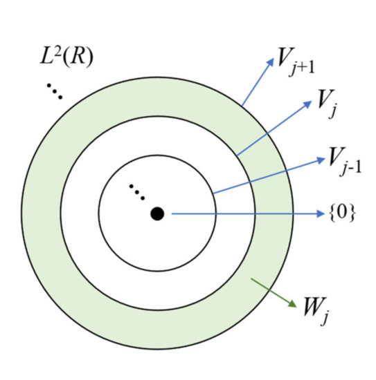
Figure 1.
Multiresolution nested space.
According to wavelet theory, similar to wavelet functions and wavelet spaces, there also exist scaling functions sj,k(x) that can construct space Vj, so that any function can be decomposed, namely
Furthermore, Equation (18) can also be written as
where Z can be any positive integer. In this way, a function on L2(R) can be represented by scaling functions and wavelet functions at any resolution. More specifically, scaling functions approximate the general information, while wavelet functions describe details at certain scales. In this paper, we utilize scaling functions as the basis function in our finite-element method for two reasons. The first is that BSWI scaling functions can accurately hold the general information at a given scale, which means that the unknown field inside each element can be well approximated. The second is that the space {Vj} constructed by scaling functions is a set of nested multiresolution spaces, so that it is natural and direct for us to enhance the scale of the basis functions and we can approximate the unknown field at a detailed resolution.
The B-spline wavelet on the interval is normally defined on a knot sequence on the reference interval (0, 1) and any function f(x) on the interval (a, b) can be mapped to the interval (0, 1) by a simple transformation formula . In general, for a given scale j () and order m, the interval (0, 1) is divided into 2j segments, then m−1 knots are added to each endpoint as virtual multi-knots to describe the information at the boundary. In this way, the knot sequence with a total number of 2j + 2m−1 is obtained. B-spline polynomials are then formed between these knots. Subsequently, BSWI can be constructed by joining these B-spline polynomials together. Note that to avoid confusing BSWI with the electric scalar potential , we use s and w in this paper to represent the scaling functions and wavelet functions of BSWI, respectively.
The BSWI basis at different scales can be transformed into each other because they satisfy a recursive relationship [42]. Taken as an example, Goswami et al. (1995) gave the expressions of the BSWI basis at 0th scale and mth order [44]. Thus, the jth scale and mth order of BSWI (simply denoted as BSWImj) scaling functions and the corresponding wavelet functions can be evaluated by the following equations:
In this paper, we set j = 1 to be the initial scale. The scaling functions and wavelet functions at all scales can be calculated according to Equation (20a,b). There are m−1 0-boundary and 1-boundary scaling functions and wavelet functions, and 2j−m + 1 inner scaling functions and 2j−2m + 2 wavelet functions (only wavelet functions at the 1st scale do not satisfy the index in Equation (20b), because they do not contain any inner wavelet functions). After we have obtained the BSWImj basis, the scaling functions and the wavelet functions on (0, 1) can be written in vector format as
It must be pointed out that the boundary BSWI basis are different from the inner ones, so that the truncated boundary can be properly described. Meanwhile, the BSWI basis has local support, which means that each scaling function or wavelet function can only affect a part of the interval (0, 1). The advantage is that the boundary can be well approximated no matter how high the scale increases. On the contrary, the conventional FEM interpolation that uses polynomials defined on the whole interval can cause a strong oscillation as the order of polynomials keeps increasing. Thus, our method can avoid the so-called Runge phenomenon.
Figure 2 shows the linear (i.e., m = 2) scaling functions and the wavelet functions at 1st scale and 2nd scale. We use the linear scaling functions in this paper as the basis functions in WFEM to approximate the unknown fields and to make the coefficient matrix sparse. We define n = 2j + m−1, which means the number of BSWI nodes for a given order and scale.
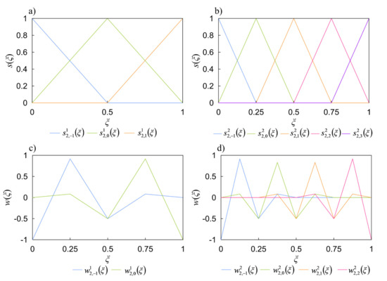
Figure 2.
Linear (m = 2) scaling functions and wavelet functions of BSWI: (a) scaling functions at scale j = 1; (b) scaling functions at scale j = 2; (c) wavelet functions at scale j = 1; (d) wavelet functions at scale j = 2.
Tensor product is a simple and direct way to construct BSWI basis on higher dimensions. Higher-dimensional BSWI basis naturally inherits all the characteristics from 1D BSWI basis. Moreover, this strategy can also form a nested multiresolution framework on higher dimension as the scale j varies (same as that shown in Figure 1). The scaling function s and the tensor product subspace Fj for 3D cases can be written as
where denotes the vector combined by scaling functions on axis, while s2 and s3 are defined on and axis, and denotes the Kronecker symbol.
Based on this discussion, 2D and 3D scaling functions are shown in Figure 3 and Figure 4. To avoid confusion, we renumbered them from 1 to n2 for 2D case and from 1 to n3 for 3D case. Figure 3 shows the 2D BSWI scaling functions at the corner (Figure 3a,d), inside (Figure 3b,e), and on the edge (Figure 3c,e) at scale j = 1 and j = 2. Figure 4 shows the 3D BSWI scaling functions at the corner (Figure 4a,e), on the edge (Figure 4b,f), on the surface (Figure 4c,g) and inside (Figure 4d,h) at scale j = 1 and j = 2.
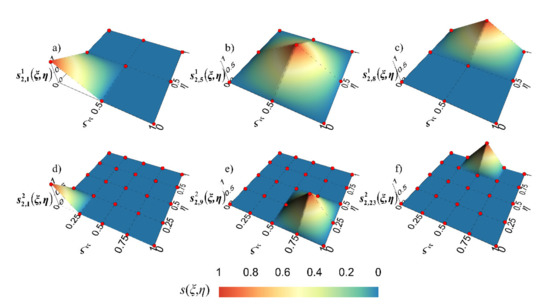
Figure 3.
2D linear BSWI basis at 1st scale (the upper row) and 2nd scale (the under row): (a)
; (b) ; (c) ; (d) ; (e) ; (f) .
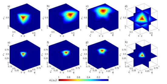
Figure 4.
3D linear BSWI basis at 1st scale (the upper row) and 2nd scale (the under row): (a) ; (b) ; (c) ; (d) ; (e) ; (f) ; (g) ; (h) .
2.3. BSWI Based Wavelet Finite-Element Method
In traditional finite-element method, the basis functions (also known as shape functions) are normally used to describe the unknown field function in each element, i.e.,
where N denotes the basis function vector, while ue is a column vector that denotes the physical degree of freedom (DOF).
As for the WFEM, according to Equation (18), any unknown function in a given hexahedral element can be mapped into a reference mesh and approximated by 3D scaling functions at scale j, namely
where represents the unknown function in the reference hexahedral domain, while denotes the wavelet coefficients column vector. In order to convert the modeling problem from wavelet domain to physical domain, which can be understood as a bridge between Equations (23) and (24), we introduce the following transformation matrix:
where T is the transformation matrix, R can be calculated from the following equations:
Note that the transformation matrix describes the value of scaling functions on each node in the reference mesh that can be simply taken as a wavelet transform. Thus, we have
The above procedure constructs the connection between the DOFs in physical space and the wavelet coefficients in the wavelet space. Equation (24) can be further expressed as
where is the basis function vector in WFEM.
So far, we have established the basis function of the BSWI-based WFEM method. The following parts of WFEM are similar to conventional FEM, and will be discussed it in the next section.
Figure 5a shows the layout and corresponding local index of nodes in the reference mesh for scale j and order m, while Figure 5b,c shows the BSWI21 and BSWI22 elements. Note that the layout of nodes is the same as that in the 3D BSWI basis, however, the basis functions are not exactly the same as the 3D BSWI basis functions because of the transformation matrix.
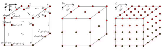
Figure 5.
Layout of 3D BSWI elements: (a) BSWImj element; (b) BSWI21 element; (c) BSWI22 element.
2.4. WFEM Analysis
In this section, we expand the vector potential A in the governing Equation (9a,b) into x, y, z components and obtain the following equations:
and we discretize by presenting them in weak format as
where . Then, we use the basis function of WFEM in Equations (24) and (29) to present the unknown potentials. For each mesh containing n3 nodes, the weak format can be represented as a linear equation Keue = be, where Ke is a complex symmetric matrix:
where the elements can be written as
while the right-hand side can be written as
where Epx, Epy, Epz are the primary electrical field column vector in x, y, and z directions. As mentioned before, we assume the primary field to be excited by a transmitting source in the free-air space, so we have for a vertical magnetic dipole (VMD) the electrical field:
where m denotes the dipole moment, , x, y, z are the relative distances between the source and the receiver at the x-, y-, and z- axis, .
In the above equations, the 3D integrations of the basis function can reduce to the tensor product of 1D integrations of the BSWI basis in the reference domain because the scaling functions in different directions are orthogonal to each other. We take the first term in Equation (33a) as example to illustrate this process. In fact, from Equation (33a), we can expand the first term as
where lx, ly, lz are the mesh sizes in physical space at x-, y-, z-axis. Similarly, the other integrations shown in Equation (33a–h) can also be written as
The 1D integration of scaling functions, wavelet functions or their derivatives in WFEM is normally called connection coefficients. We use to represent these connection coefficients, where p and q denote the order of the derivate of the scaling functions, while d represents the axis. In this paper, the following four connection coefficients are used (only those on axis are shown as examples).
In much existing research on WFEM that apply wavelets (e.g., the DB wavelet) as the basis functions, the calculation of connection coefficients can be a challenging problem [57,58]. The definition on the whole real axis and the lack of explicit expressions, as mentioned above, are the most important issues. In this paper, due to the explicit expression and the definition on the interval (0, 1) of BSWI, we can easily obtain the explicit solutions of connection coefficients. In Appendix A, we have given the expressions of connection coefficients for m = 2, j = 1 and m = 2, j = 2.
Finally, the element matrix and right-hand side for each element is formed and integrated together and then the Dirichlet boundary condition is applied, so that we can get the following global linear system for our forward modeling problem, i.e.,
As we have discussed before, one reason why wavelet is frequently utilized in numerical methods is that it can make the matrix sparse, as does the BSWI basis. The BSWI has local support, which means that each scaling function can only affect a limited area in the mesh. This will further create fewer non-zero coefficients in the matrix. Figure 6 shows the sparsity pattern of the element matrix and global matrix formed by BSWI21 and BBSWI22 elements. From the figures it is seen that the BSWI indeed contributes to a sparser matrix; the non-zero coefficients are concentrated around the diagonal, so that a lower time consumption can be expected. We will discuss this via numerical experiments in next section.
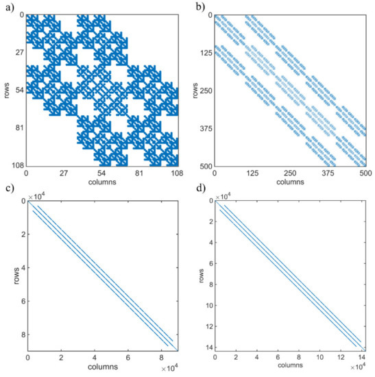
Figure 6.
Sparsity pattern of the BSWI-based WFEM: (a) element matrix of BSWI21 elements; (b) element matrix of BSWI22 elements; (c) global matrix when using BSWI21 elements; (d) global matrix when using BSWI22 matrix.
Airborne EM modeling is a multi-source problem because the airborne transmitter keeps moving during the survey. To solve the linear equations system efficiently, we use the direct solver MUMPS [59,60]. This method needs only to do the factorization once and replace the source term at the right-hand side for moving transmitters.
2.5. Moving Least-Squares Interpolation
In this section, we apply a moving least-squares interpolation (MLSI) scheme introduced by Tabbara et al. (1994) to recover EM fields Es and Hs from the secondary potentials As and [61]. For this purpose, we assume that each component of the secondary vector potential As and the scalar potential can be approximated by a linear function that can be written as
where u* is the approximate linear function, is the variable vector, while is the column vector composed of unknown coefficients. The coefficients vector is determined by minimizing the weighted differences between u* and the computed potential u taking the nearest N nodes to the receiver into account, namely
where is the weighted function, d is the distance from the node to the receiver, and h = max(d). N is usually set to be 30~50. The MLSI assures that the derivatives are smooth and accurate so that the EM fields can be well recovered.
3. Numerical Experiments
3.1. Accuracy Verification
In this section, we first simulate as an example the EM responses of a horizontal coplanar (HCP) AEM system over a homogeneous half-space model to verify the accuracy of our method. The Tx-Rx offset is assumed to be 10m. The flight attitude is 30 m. The earth resistivity is ohm-m. Here, three mesh discretization cases are considered to illustrate how the accuracy can be improved when we refine the mesh or enhance the scale. The model is divided into , and elements, labeled as Case 1, Case 2, and Case 3, in which , and elements are taken as the calculation domain. Meanwhile, the outer boundary is extended 6000 m in each direction. We calculate 21 logarithmically equal-spaced frequencies ranging from 100 Hz to 215 kHz. The results are compared to the 1D semi-analytic solutions calculated using the code from Yin and Fraser [62]. From Figure 7, it is seen that our method obtains high accuracy with only a small number of meshes. For BSWI21 elements in Case 1, the relative errors of both the real and the imaginary part are not able to meet our needs. The maximum relative error can be up to about 15%. This is simply because the mesh discretization is too rough. After the mesh refinement from Case 1 to Case 2, we can see that the relative error shows a sharp reduction, with the relative error reduced to less than 5%. Meanwhile, the time cost is only about 15 s for one frequency (see Table 1). For comparison purposes, we further refine the mesh to Case 3. The result shows that in this case the relative error of the real part becomes less than 1% for most frequencies, while the error of the imaginary part is lower than that of the real part with a maximum value of 1%. This indicates that the results from our method are very accurate. As for the BSWI22 elements, the relative error in Case 1 is already under 1% for most frequencies. However, at very high frequencies the error keeps rising to about 8%. However, after the mesh is refined in Case 2, we can obtain similar accuracy as that in Case 3 using BSWI21 elements. The maximum relative error of the real part is about 3% at 215 kHz while that of the imaginary part is under 0.6% at all frequencies. This indicates again that the accuracy can be improved when the scale of BSWI basis is increased. From Table 1 it is seen that the BSWI22 elements lead to a system with more DOFs than BSWI21 elements. As a result, the corresponding time cost becomes higher. Since the results are accurate enough, we do not continue refining the mesh. From this example, we can obviously see that the BSWI-based WFEM depends less on meshes so that one can simulate the EM response with fewer meshes than the conventional FEM. At the same time, as the high-scale functions can describe the unknown field at high resolutions, so we can improve the accuracy by increasing the scale. This provides double tracks for improving the accuracy in our modeling process.
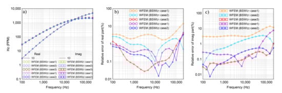
Figure 7.
Accuracy verification by comparing our WFEM results with semi-analytical solutions for a homogenous half-space model: (a) comparison of EM responses; (b) relative error of the real part; (c) relative error of the imaginary part.

Table 1.
BSWI basis selection, mesh subdivision, and time consumption of WFEM for a half-space model.
In the following discussion, we use a layered earth model to further illustrate the efficiency and accuracy of our method. The model is shown in Figure 8. The system parameters are the same as the half-space model in Figure 7. For comparison purposes, we use two methods of the nodal-based FEM and the edge-based FEM [12] (abbreviated as nFEM and eFEM in the following figures, respectively). Here, we use the edge-based FEM to solve the curl-curl equation for the electric field E while we use the nodal-based FEM to solve the coupled potentials A and . Note that in our comparison the time consumption is taken as the total time, including the time for the factorization and solution. The model used for these three methods is set to be 650 m × 650 m × 550 m with the Tx-Rx system located at its center. We use BSWI21 meshes to do the forward modeling. To make the comparison, two mesh subdivision cases are respectively applied to nodal-based FEM and edge-based FEM. In Case 1, after the mesh subdivision, the DOFs of the three methods are similar (see Table 2). Figure 9 shows the EM responses. From Figure 9b,c one sees that the relative error of WFEM to the semi-analytical solutions is the lowest, which is under 1% at most frequencies for both the real and imaginary parts. Meanwhile, the time consumption is between that of the nodal-based and edge-based FEM. The solutions obtained by the edge-based FEM have the lowest accuracy, the relative error of the imaginary part exceeds 5% at high frequencies. Finally, the nodal-based FEM takes a longer time than our WFEM to provide a solution at low accuracy, which further indicates that WFEM can obtain more accurate results with less time than conventional FEM. In Case 2, we further refine the mesh in Case 1. The details of the mesh subdivision and time consumption are shown in Table 2. From the result comparison and the relative error in Figure 9, one can see that the mesh refinement does improve the accuracy. For edge-based FEM, the accuracy improvement is apparent. However, although the time consumption has been raised to the same level as that of WFEM, the accuracy is still far lower than that of WFEM. As for the nodal-based FEM, the mesh refinement near the system does not contribute much to the accuracy improvement of the real part, but it improves the imaginary part. Thus, we can conclude that the BSWI basis shows better performance than the conventional polynomial interpolation as it captures more local details and the information on the boundaries of meshes. In addition, it contributes to a sparser matrix and thus speeds up the solution of the linear equations. Although the vector basis functions can satisfy the divergence condition in each element, the edge-based FEM still shows less stability than our nodal-based WFEM using coupled-potential formulation.
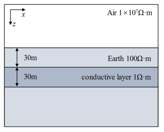
Figure 8.
A layered earth model.
Table 2.
Mesh subdivision and time consumption of WFEM, edge-based FEM and nodal-based FEM for the layered earth model in Figure 8.
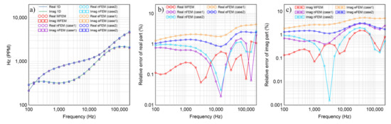
Figure 9.
Comparison of WFEM, the edge-based and nodal-based FEM for the model in Figure 8: (a) comparison of EM responses; (b) relative error of the real part; (c) relative error of the imaginary part.
3.2. 3D Synthetic Models
In this section, we first assume a synthetic Example 1 with a 1 ohm-m conductive body embedded in a 100 ohm-m half-space for our modeling. The size of the conductive body is 80 m × 80 m × 20 m with a top depth of 40 m. The coordinate of its central point is (0 m, 0 m, 50 m). The system parameters are the same as the previous models. We calculate the HCP system responses for a total of 31 Tx-Rx locations along the survey line y = 0 m ranging from x = −150 m to 150 m. The transmitting frequencies are 380, 1600, 6300, and 25,000 Hz, respectively. To illustrate the influence of the BSWI scale and mesh size on the accuracy, we adopt four different subdivisions to discretize the model domain. We use BSWI21 elements to divide the model into mesh for Case 1 and 2, while we use BSWI22 elements to divide the model for Case 3 and 4. In Case 1, the maximum size of 40 m × 40 m × 40 m is assumed. In Case 2, a mesh refinement is applied to the model without changing the scale of BSWI basis. In Case 3, the scale is increased to j = 2 while the mesh is still the same as in Case 1. In Case 4, the mesh is refined, and the scale is increased. The EM responses are shown in Figure 10, respectively, while the time consumptions are given in Table 3. For easy comparison, we also present the EM responses calculated by the spectral element method (SEM). According to [63], as a high-order numerical algorithm, SEM has proved to be very accurate. Here, we use the third order of Gauss–Lobatto–Chebyshev (GLC) polynomials as the basis function of SEM for the mesh size of 20 m × 20 m × 20 m. It is seen from Figure 10 that the model in Case 1 failed to obtain reasonable results, as a large difference between Case 1 and SEM can be observed. Table 3 shows the maximum relative errors between our results and the SEM solutions for four cases. It is seen that the maximum relative error between these two methods is 17.4% at 25,000 Hz. This means that the results in Case 1 are not reliable. Meanwhile, the response at high frequencies shows a dramatic oscillation. This is because as the frequency increases, the EM field varies quickly, so that it becomes harder for a rough mesh to simulate. To improve the accuracy, we apply in Case 2 a mesh refinement. Apparently, the results of Case 2 become smoother and closer to the SEM responses, and the relative error drops at all frequencies with a maximum of 4.01%. Similar results can be observed in Case 3, where we enhance the scale of the basis function on the bases of Case 1. Using BSWI22 elements, the relative error falls down when compared to Case 1 and 2 except for the real part of 25,000 Hz (see Figure 11). Among all frequencies, the maximum relative error is 3.43%. Finally, we apply both the mesh refinement and scale enhancement to Case 1. It is seen that the accuracy is largely improved. The maximum relative error between Case 4 and SEM falls to 3.02%. This confirms again that in our new algorithm, we can improve the modeling accuracy by mesh refinement and the scale enhancement.
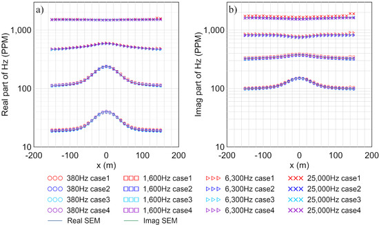
Figure 10.
EM responses obtained from 4 cases of Example 1 compared to SEM results: (a) real part; (b) imaginary part.
Table 3.
Scale of basis function, mesh subdivision, time consumption, and maximum relative error for 4 cases of Example 1.
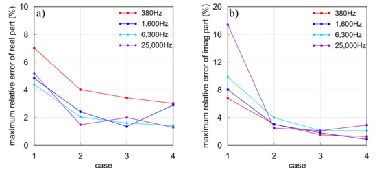
Figure 11.
The maximum relative errors between WFEM and SEM for Example 1 at different frequencies: (a) real part; (b) imaginary part.
We then simulate the responses of Example 2 to verify whether our method can handle high resistivity contrast. The model is the same as that in Example 1 except for that the resistivity contrast becomes 0.1 ohm-m for the anomalous body to 500 ohm-m for the half-space. Meanwhile, the same four subdivisions are used to discretize the model and the result from SEM is used as comparison. Figure 12 shows the EM responses, while Table 4 gives the time consumption. From Figure 12 and Figure 13, one can draw similar conclusions to the previous example that with the mesh refinement and scale increasing, the relative errors between our results and the SEM results decrease. The maximum relative error is reduced from 34.8% in Case 1 to about 6% in Case 2 and 3, and to 4.41% in Case 4. Note that the relative error in this example is higher than that in the previous example. This is because when the resistivity contrasts across surfaces become high, the EM field changes sharply. As a result, the accuracy of numerical algorithms is reduced. Even so, our method can still obtain reliable results.
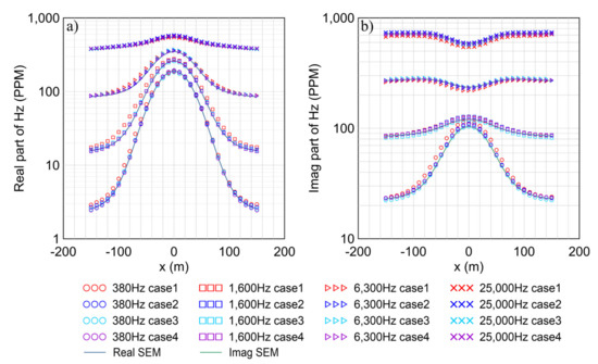
Figure 12.
EM responses obtained from 4 cases of Example 2 compared to SEM results: (a) real part; (b) imaginary part.
Table 4.
Scale of basis function, mesh subdivision, time consumption, and maximum relative error for 4 cases of Example 2.
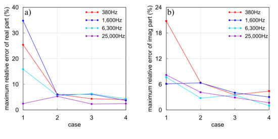
Figure 13.
The maximum relative errors between WFEM and SEM for Example 2 at different frequencies: (a) real part; (b) imaginary part.
4. Conclusions
In this paper, we have successfully developed the wavelet finite-element method based on the B-spline wavelet on the interval for 3D frequency-domain airborne EM modeling. The BSWI, as the basis function, can better approximate the field variation than the conventional polynomial basis function. Due to special design on the boundary and local support, our method can avoid the Runge phenomenon at high scales, since this method creates a sparser matrix than the traditional FEM method so that the efficiency can be improved. Comparison with 1D semi-analytical solutions validates our method. The numerical experiments for typical models demonstrated that our method has higher accuracy and efficiency than conventional FEM methods. As a high-order numerical method, our algorithm is more flexible in that it is less dependent on the mesh subdivision. Moreover, our method can improve the accuracy by either refining the mesh or increasing the scale of BSWI basis. This obviously offers us more possibilities for accurate numerical modeling and inversions. More specifically, we can use coarse meshes and low-scale BSWI basis functions in the early iterations of the inversion process to recover the rough structure of the underground. With increasing iteration steps, we can use finer meshes and higher-scale BSWI basis to improve the resolution of the inversion continuously, so that we can obtain a steady solution. We must point out that the study in this paper is still preliminary. The structured hexahedral mesh has limitations in fitting the topography or complex underground structures. An unstructured mesh is without doubt the best choice. In addition, the p-type adaptive algorithm that allows local scale enhancement and 3D inversions that adapt to the flexibility of our method are of great attraction to our research. All these will be our future research focus.
Author Contributions
Conceptualization, L.G., C.Y. and Y.L.; Formal analysis, L.G., C.Y., X.R., B.Z. and B.X.; Funding acquisition, C.Y. and B.Z.; Investigation, L.G. and N.W.; Methodology, L.G., J.Z. and Y.L.; Software, L.G.; Visualization, L.G. and N.W.; Writing—original draft, L.G.; Writing—review & editing, L.G. and C.Y. All authors have read and agreed to the published version of the manuscript.
Funding
This paper is financially supported by the National Natural Science Foundation of China (42030806, 41804098, 42074120, 41904104, 41774125).
Conflicts of Interest
The authors declare no conflict of interest.
Appendix A. The Connection Coefficients
Since the BSWI in Equation (20) has explicit expressions, the calculation of connection coefficients is simple. In this section, we will give the expressions of four types of connection coefficients at different scales. For BSWI21 elements, all connection coefficients are matrix that can be written as
In the case of BSWI22 elements, the connection coefficients are all matrix, which are
.
References
- Pfaffhuber, A.A.; Monstad, S.; Rudd, J. Airborne electromagnetic hydrocarbon mapping in Mozambique. Explor. Geophys. 2009, 40, 237–245. [Google Scholar] [CrossRef]
- Tan, K.; Munday, T.; Halas, L.; Cahill, K. Utilizing airborne electromagnetic data to map groundwater salinity and salt store at Chowilla, SA. ASEG Ext. Abstr. 2009, 2009, 1–6. [Google Scholar] [CrossRef]
- Yang, D.K.; Oldenburg, D.W. 3D conductivity models of Lalor Lake VMS deposit from ground loop and airborne EM data sets. In Proceedings of the 23rd International Geophysical Conference and Exhibition, Melbourne, Australia, 11–14 August 2013. [Google Scholar]
- Wolfgram, P.; Golden, H. Airborne EM applied to sulphide nickel-examples and analysis. Explor. Geophys. 2001, 32, 136–140. [Google Scholar] [CrossRef]
- Hodges, G.; Aniston, C. Airborne Geophysics applied to Engineering and Environmental Problems. In Proceedings of the International Conference on Engineering Geophysics, Al Ain, United Arab Emirates, 15–18 November 2015. [Google Scholar]
- Siemon, B.; Seht, M.; Steuer, A.; Deus, N.; Wiederhold, H. Airborne Electromagnetic, Magnetic, and Radiometric Surveys at the German North Sea Coast Applied to Groundwater and Soil Investigations. Remote Sens. 2020, 12, 1629. [Google Scholar] [CrossRef]
- Best, M.E.; Levson, V.M.; Ferbey, T.; McConnell, D. Airborne electromagnetic mapping for buried quaternary sands and gravels in northeast British Columbia, Canada. J. Environ. Eng. Geophys. 2006, 11, 17–26. [Google Scholar] [CrossRef]
- Avdeev, D.B.; Kuvshinov, A.V.; Pankratov, O.V.; Newman, G.A. Three-dimensional frequency-domain modeling of airborne electromagnetic responses. Explor. Geophys. 1998, 29, 111–119. [Google Scholar] [CrossRef]
- Newman, G.A.; Alumbaugh, D.L. Frequency-domain modelling of airborne electromagnetic responses using staggered finite differences1. Geophys. Prospect. 1995, 43, 1021–1042. [Google Scholar] [CrossRef]
- Liu, Y.; Yin, C. 3D anisotropic modeling for airborne EM systems using finite-difference method. J. Appl. Geophys. 2014, 109, 186–194. [Google Scholar] [CrossRef]
- Yin, C.; Zhang, B.; Liu, Y.; Cai, J. A goal-oriented adaptive finite-element method for 3D scattered airborne electromagnetic method modeling. Geophysics 2016, 81, 337–346. [Google Scholar] [CrossRef]
- Huang, W.; Yin, C.; Ben, F.; Liu, Y.; Chen, H.; Cai, J. 3D forward modeling for frequency AEM by vector finite element. Earth Sci. 2016, 41, 331–342. (In Chinese) [Google Scholar]
- Yee, K.S. Numerical solution of initial boundary value problems involving maxwell’s equations in isotropic media. IEEE Trans. Antennas Propag. 1966, 14, 302–307. [Google Scholar]
- Yin, C.; Huang, X.; Liu, Y.; Cai, J. 3-D modeling for airborne EM using spectral-element method. J. Environ. Eng. Geophys. 2017, 22, 13–23. [Google Scholar] [CrossRef]
- Octavio, C.R.; Josep, D.L.P.; Emilio, G.C.; José, M.C. Parallel 3D marine controlled-source electromagnetic modelling using high-order tetrahedral Nédélec elements. Geophys. J. Int. 2019, 219, 39–65. [Google Scholar]
- Schwarzbach, C.; Börner, R.; Spitzer, K. Three-dimensional adaptive higher order finite element simulation for geo-electromagnetics-a marine CSEM example. Geophys. J. Int. 2011, 187, 63–74. [Google Scholar] [CrossRef] [Green Version]
- Runge, C. Über empirische Funktionen und die Interpolation zwischen äquidistanten Ordinaten. Z. Math. Phys. 1901, 46, 224–243. [Google Scholar]
- Morlet, J.; Arens, G.; Fourgeau, E.; Giard, D. Wave propagation and sampling theory-Part II: Sampling theory and complex waves. Geophysics 1982, 47, 222–236. [Google Scholar] [CrossRef]
- Meyer, Y. Principe d’incertitude, bases hilbertiennes et algèbres d’opérateurs. Semin. Bourbaki Paris 1986, 4, 209–223. [Google Scholar]
- Grossmann, A.; Morlet, J. Decomposition of Hardy Functions into Square Integrable Wavelets of Constant Shape. SIAM J. Math. Anal. 1984, 15, 723–736. [Google Scholar] [CrossRef]
- Mallat, S.G. Multiresolution approximations and wavelet orthonormal bases of L2(R). Trans. Am. Math. Soc. 1989, 315, 69–87. [Google Scholar]
- Daubechies, I. Orthonormal bases of compactly supported wavelets. Commun. Pure Appl. Math. 1989, 3115, 69–81. [Google Scholar]
- Sweldens, W. The Lifting Scheme: A Custom-Design Construction of Biorthogonal Wavelets. Appl. Comput. Harmon. Anal. 1996, 3, 186–200. [Google Scholar] [CrossRef] [Green Version]
- Donoho, D.L.; Johnstone, I.M. Ideal spatial adaptation by wavelet shrinkage. Biometrika 1994, 81, 425–455. [Google Scholar] [CrossRef]
- Mallat, S.G. A Wavelet Tour of Signal Processing; Academic Press: Cambridge, MA, USA, 1999. [Google Scholar]
- Plattner, A.; Maurer, H.R.; Vorloeper, J.; Blome, J. 3-D electrical resistivity tomography using adaptive wavelet parameter grids. Geophys. J. Int. 2012, 189, 317–330. [Google Scholar] [CrossRef] [Green Version]
- Liu, Y.; Farquharson, C.G.; Yin, C.; Vikas, C.B. Wavelet-based 3D inversion for frequency-domain airborne EM data. Geophys. J. Int. 2017, 213, 1–15. [Google Scholar] [CrossRef]
- Christensen, N. Interpretation attributes derived from airborne electromagnetic inversion models using the continuous wavelet transform. Near Surf. Geophys. 2018, 16, 665–678. [Google Scholar] [CrossRef]
- Hustdet, B.; Operto, S.; Virieux, J. A multi-level direct-iterative solver for seismic wave propagation modelling: Space and wavelet approaches. Geophys. J. Int. 2003, 155, 953–980. [Google Scholar] [CrossRef] [Green Version]
- Chakraborty, A.; Okaya, D. Frequency-time decomposition of seismic data using wavelet-based methods. Geophysics 1995, 60, 1906–1916. [Google Scholar] [CrossRef] [Green Version]
- Amaratunga, K.; Williams, J.R. Wavelet based Green’s function approach to 2D PDEs. Eng. Comput. 1993, 10, 349–367. [Google Scholar] [CrossRef] [Green Version]
- Cohen, A.; Kaber, S.M.; Postel, M. Adaptive multiresolution for finite volume solutions of gas dynamics. Comput. Fluids 2003, 32, 31–38. [Google Scholar] [CrossRef]
- Sarkar, T.K.; Adve, R.S.; Garcia-Castillo, L.E.; Salazar-Palma, M. Utilization of wavelet concepts in finite elements for an efficient solution of Maxwell’s equations. Radio Sci. 1994, 29, 965–977. [Google Scholar] [CrossRef]
- Castro, L.M.; Barbosa, A.R. Implementation of an hybrid-mixed stress model based on the use of wavelets. Comput. Struct. 2006, 84, 718–731. [Google Scholar] [CrossRef]
- Zhang, X.; Liu, K.; Liu, J. A wavelet finite element method for the 2D wave equation in fluid-saturated porous media. Chin. J. Geophys. 2005, 48, 1156–1166. [Google Scholar] [CrossRef]
- Feng, D.; Yang, B.; Wang, X.; Du, H. Daubechies wavelet finite element method for solving the GPR wave equations. Chin. J. Geophys. 2016, 59, 342–354. [Google Scholar]
- Hussain, N.; Karsiti, M.N.; Joeti, V.; Yahya, N. Use of wavelets in marine controlled source electromagnetic method for geophysical modeling. Int. J. Appl. Electromagn. Mech. 2016, 51, 431–443. [Google Scholar] [CrossRef]
- Hussain, N.; Karsiti, M.N.; Yahya, N.; Joeti, V.; Yahya, N. 2D wavelets galerkin method for the computation of EM field on seafloor excited by a point source. Int. J. Appl. Electromagn. Mech. 2017, 53, 631–644. [Google Scholar] [CrossRef]
- Chen, H.; Li, T. 3D marine controlled-source electromagnetic modelling in an anisotropic medium using a Wavelet–Galerkin method with a secondary potential formulation. Geophys. J. Int. 2019, 219, 373–393. [Google Scholar] [CrossRef]
- He, Y.; Chen, X.; Xiang, J.; He, Z. Adaptive multiresolution finite element method based on second generation wavelets. Finite Elem. Anal. Des. 2007, 43, 566–579. [Google Scholar] [CrossRef]
- Castro, L. Polynomial wavelets in hybrid-mixed stress finite element models. Int. J. Numer. Methods Biomed. Eng. 2010, 26, 1293–1312. [Google Scholar] [CrossRef]
- Chui, C.K.; Quak, E. Wavelets on a bounded interval. In Numerical Methods in Approximation Theory; Birkhäuser: Basel, Switzerland, 1992; Volume 9, pp. 53–75. [Google Scholar]
- Schoenberg, J. Contribution to the problem of approximation of equidistant data by analytic functions. Quart. Appl. Math. 1946, 4, 112–141. [Google Scholar] [CrossRef] [Green Version]
- Goswami, J.C.; Chan, A.K.; Chui, C.K. On solving first-kind integral equations using wavelets on a bounded interval. IEEE Trans. Antennas Propag. 1995, 43, 614–622. [Google Scholar] [CrossRef]
- Xiang, J.; Chen, X.; He, Y.; He, Z. The construction of plane elastomechanics and Mindlin plate elements of B-spline wavelet on the interval. Finite Elem. Anal. Des. 2006, 42, 1269–1280. [Google Scholar] [CrossRef]
- Shen, W.; Li, D.; Ou, J. Dispersion Analysis of Multiscale Wavelet Finite Element for 2D Elastic Wave Propagation. J. Eng. Mech. 2020, 146, 04020022. [Google Scholar] [CrossRef]
- Feng, D.; Wang, X.; Zhang, B.; Ren, Z. An investigation into the electromagnetic response of porous media with GPR using stochastic processes and FEM of B-spline wavelet on the interval. J. Appl. Geophys. 2019, 169, 174–182. [Google Scholar] [CrossRef]
- Barton, M.L.; Cendes, A.J. New vector finite elements for three-dimensional magnetic field computation. J. Appl. Phys. 1987, 61, 3919–3921. [Google Scholar] [CrossRef]
- Biro, O.; Preis, K. On the use of the magnetic vector potential in the finite element analysis of the three-dimensional eddy currents. IEEE Trans. Magn. 1989, 25, 3145–3159. [Google Scholar] [CrossRef]
- Nédéléc, J.C. Mixed finite element in R3. Numer. Math. 1980, 35, 315–341. [Google Scholar] [CrossRef]
- Ward, S.H.; Hohmann, G.W. Electromagnetic theory for geophysical applications. In Electromagnetic Method in applied Geophysics; Society of Exploration Geophysicists: Tulsa, OK, USA, 1988; pp. 131–311. [Google Scholar]
- Badea, E.A.; Everett, M.E.; Newman, G.A.; Biro, O. Finite-element analysis of controlled-source electromagnetic induction using Coulomb-gauged potentials. Geophysics 2001, 66, 786–799. [Google Scholar] [CrossRef]
- Everett, M.E.; Schultz, A. Geomagnetic induction in a heterogeneous sphere: Azimuthally symmetric test computations and the response of an undulating 660-km discontinuity. J. Geophys. Res. Solid Earth 1996, 101, 2765–2783. [Google Scholar] [CrossRef]
- Mitsuhata, Y.; Uchida, T. 3D magnetotelluric modeling using the T-Ω method. Geophysics 2004, 69, 108–119. [Google Scholar] [CrossRef]
- Puzyrev, V.; Koldan, J.; Puente, J.; Houzeaux, G.; Vázquez, M.; Cela, J.M. A parallel finite-element method for three-dimensional controlled-source electromagnetic forward modelling. Geophys. J. Int. 2013, 193, 678–693. [Google Scholar] [CrossRef] [Green Version]
- Weiss, C.J. Project APhiD: A Lorenz-gauged A-ϕ decomposition for parallelized computation of ultra-broadband electromagnetic induction in a fully heterogeneous earth. Comput. Geosci. 2013, 58, 40–52. [Google Scholar] [CrossRef]
- Yang, S.; Ni, G. Wavelet-Galerkin method for computations of electromagnetic fields-computation of connection coefficients. IEEE Trans. Magn. 2000, 36, 644–648. [Google Scholar] [CrossRef] [Green Version]
- Lin, E.; Zhou, X. Connection coefficients on an interval and wavelet solutions of Burgers equation. J. Comput. Appl. Math. 2001, 135, 63–78. [Google Scholar] [CrossRef] [Green Version]
- Amestoy, P.R.; Duff, I.S.; L’Excellent, J.Y.; Koster, J. A fully asynchronous multifrontal solver using distributed dynamic scheduling. SIAM J. Matrix Anal. Appl. 2001, 23, 15–41. [Google Scholar] [CrossRef] [Green Version]
- Amestoy, P.R.; Duff, I.S.; L’Excellent, J.Y.; Robert, Y.; Rouet, F.H.; Ucar, B. On computing inverse entries of a sparse matrix in an out-of-core environment. SIAM J. Sci. Comput. 2012, 34, 1975–1999. [Google Scholar] [CrossRef] [Green Version]
- Tabbara, M.; Blacker, T.; Belytschko, T. Finite element derivative recovery by moving least square interpolants. Comput. Methods Appl. Mech. Eng. 1994, 117, 211–223. [Google Scholar] [CrossRef]
- Yin, C.; Fraser, D.C. The effect of the electrical anisotropy on the response of helicopter-borne frequency-domain electromagnetic systems. Geophys. Prospect. 2004, 52, 399–416. [Google Scholar] [CrossRef]
- Yin, C.; Liu, L.; Liu, Y.; Zhang, B.; Qiu, C.; Huang, X. 3D frequency-domain airborne EM forward modelling using spectral element method with gauss–lobatto–chebyshev polynomials. Explor. Geophys. 2019, 50, 461–471. [Google Scholar] [CrossRef]
Publisher’s Note: MDPI stays neutral with regard to jurisdictional claims in published maps and institutional affiliations. |
© 2021 by the authors. Licensee MDPI, Basel, Switzerland. This article is an open access article distributed under the terms and conditions of the Creative Commons Attribution (CC BY) license (https://creativecommons.org/licenses/by/4.0/).