Abstract
Recently, deep metric learning (DML) has received widespread attention in the field of remote sensing image retrieval (RSIR), owing to its ability to extract discriminative features to represent images and then to measure the similarity between images via learning a distance function among feature vectors. However, the distinguishability of features extracted by the most current DML-based methods for RSIR is still not sufficient, and the retrieval efficiency needs to be further improved. To this end, we propose a novel ensemble architecture of residual attention-based deep metric learning (EARA) for RSIR. In our proposed architecture, residual attention is introduced and ameliorated to increase feature discriminability, maintain global features, and concatenate feature vectors of different weights. Then, descriptor ensemble rather than embedding ensemble is chosen to further boost the performance of RSIR with reduced time cost and memory consumption. Furthermore, our proposed architecture can be flexibly extended with different types of deep neural networks, loss functions, and feature descriptors. To evaluate the performance and efficiency of our architecture, we conduct exhaustive experiments on three benchmark remote sensing datasets, including UCMD, SIRI-WHU, and AID. The experimental results demonstrate that the proposed architecture outperforms the four state-of-the-art methods, including BIER, A-BIER, DCES, and ABE, by 15.45%, 13.04%, 10.31%, and 6.62% in the mean Average Precision (mAP), respectively. As for the retrieval execution complexity, the retrieval time and floating point of operations (FLOPs), needed by the proposed architecture on AID, reduce by 92% and 80% compared to those needed by ABE, albeit with the same Recall@1 between the two methods.
1. Introduction
With the rapid development of satellite technologies, there is an urgent demand for sophisticated techniques to deal with remote sensing big data. At present, the basic and paramount tasks in remote sensing image processing include object/instance detection, classification, retrieval, object surface analysis, and segmentation, to name a few. Among these tasks, remote sensing image retrieval (RSIR), which aims to retrieve the most similar images in semantics to the query image, consists of two-stage of feature extraction and similarity metric, receives persistent attention in the remote sensing community [1,2,3,4,5,6,7,8,9,10,11,12,13,14,15,16,17,18,19,20,21,22,23].
Remote sensing images always contain rich information on geographic location, variable scales, and semantic objects. The large-scale variance problem [4,5] makes it difficult to describe semantic information hidden in remote sensing images. During past several decades, a variety of methods has been developed to extract low-level, mid-level, and high-level visual features for RSIR [6,7]. Among them, early works focused on designing hand-crafted descriptors to represent visual features [6,7,8,9,10], which are not sufficient to represent the latent semantic meaning. The design of hand-crafted feature requires sufficient professional knowledge and is time-consuming. In addition, the phenomenon -the same spectra from different objects and the same objects exhibiting different spectra in images can result in intraclass differences and inter-class similarities [11,12]. Compared with hand-crafted features, discriminative deep features learned through convolutional neural networks (CNNs) [7,13,14,15] to represent high-level semantic features of remote sensing images have proven to be more effective in RSIR [8].
Metric learning (ML) calculates the similarity between images by learning a distance function based on concrete tasks, rather than simply using certain pre-defined distance functions, and has been a focus in machine learning and computer vision, such as image classification and image retrieval [16,17]. Combining the advantages of deep learning and metric learning, deep metric learning (DML) extracts more semantic features, utilizes optimal distance functions, like Euclidean distance, and then clusters the vectors of similar samples together while pushing dissimilar vectors apart [18,19]. The capacity of DML to understand the similarities among the samples is manifested in its extensive applications in natural image fields such as face recognition [19] and natural image retrieval [20,21]. Due to its ascendancy over other methods, DML has been introduced in RSIR [22] to better understand the semantic similarity relationships among remote sensing images. For example, Subhanker et al. [23] pioneered a hash retrieval architecture based on DML for RSIR. In brief, the superiority of DML in RSIR can be summarized in two aspects: (1) it lessens the deviance between multiple goals of two stages and results via effective consistency of the two-stage feature extraction and similarity metric calculation, and (2) it reduces the computational complexity of RSIR originated from high-dimensional feature representation of plentiful and complex contents of remote sensing images.
To improve the RSIR performance, the popular idea introduces a network to learn discriminative embeddings, which is focused on designing loss functions, such as contrastive loss [22] and enhanced triplet loss [24]. However, the reliance on loss function in a high-dimensional embedding space only for improved RSIR performance would lead to overfitting and high-computation complexity, e.g., high FLOPs and time cost [25,26]. Meanwhile, local optimization caused by the inadequate use of sample pairs also leads to poor performance [27,28,29].
To address the problem of high-computation complexity and achieve a higher retrieval efficiency, we propose a novel ensemble architecture of residual attention-based deep metric learning (EARA). The idea of EARA is motivated by the dominance of residual attention [30] in extracting discriminative and comprehensive features. In this ensemble architecture, two branches, Main Branch and Residual Attention Branch, are designed to construct the submodule of the architecture. While the Main Branch maintains complete global features of remote sensing images, the Residual Attention Branch extracts more discriminative features and determines the subsequent dynamic calculation of feature weights. With the global and discriminative information of remote sensing images, EARA leverages semantic similarity relationships among samples to boost performances and simultaneously alleviate the problems of network attenuation and gradient disappearance caused by simply stacking attention modules and deep layers. Residual attention has a top-down feedforward structure, which can integrate different types of attention to obtain global discriminative image features and assign soft weights to the obtained features to improve feature discrimination. In this study, EARA improves the image retrieval performance by reducing the number of residual attention modules from three to one and placing the module in the Stage 4 of ResNet50 instead of the original Stages 1, 2, and 3. This revised configuration of residual attention maintains the structural information without stacking many layers for computation and, thus, speeds up the convergence and reduces the FLOPs and time cost. EARA also utilizes an ensemble method to concatenate submodules to encourage a rich diversity of features. To our best knowledge, this study is the first attempt to use descriptor ensemble rather than embedding ensemble to help reduce time and memory cost in the training phase for RSIR.
Ablation experiments are conducted on three benchmark remote sensing datasets, UCMD [31], SIRI-WHU [32], and AID [33]. A comparative analysis is provided in reference to the SOTA methods, including BIER [34], A-BIER [35], DCES [36], and ABE [37]. The experimental results demonstrate that our architecture has a better retrieval performance with reduced computational complexity. Specifically, EARA achieves gains of 11.46%, 9.75%, and 6.62% in mAP on UCMD [31], SIRI-WHU [32], and AID [33], respectively, compared to the second-ranked ABE. In the best case, EARA reduces the retrieval time and the FLOPs to nearly 20% and 8% of ABE on AID, which shows the superiority of our architecture in retrieval execution. Additionally, our architecture can be easily extended with other types of deep neural networks and loss functions. In general, EARA enhances the RSIR performance with the combination of complete global information and distinctive region information. The main contributions of this paper can be summarized in three aspects.
- A novel architecture of residual attention-based deep metric learning is developed, in which residual attention is improved in number and position as the Residual Attention Branch obtains more distinctive features. Meanwhile, global features extracted from the Main Branch are maintained to learn more similarity relationships among remote sensing images without extra parameters. Additionally, the dynamic weighted feature vectors in the subsequent similarity metric stage are also conditional on the feature discrimination, optimizing the retrieval results.
- The traditional ensemble method is improved by merging multiple descriptors rather than embedding the subspace to further encourage the distinguishability of remote sensing features to ultimately improve the RSIR performance. Merging descriptors decrease the computational complexity in the embedding space and significantly reduces the time and memory consumption during the training phase.
- By training the proposed model in an end-to-end manner, exhaustive experiments are conducted on three remote sensing benchmark datasets: UCMD [31], SIRI-WHU [32], and AID [33]. Comparisons of the proposed method with the SOTA methods BIER [34], A-BIER [35], DCES [36], and ABE [37] demonstrate that EARA reduces the retrieval time and FLOPs to nearly 20% and 8% of ABE on AID.
The related work for DML-based and/or attention methods for RSIR is described in Section 2. More details of the architecture of EARA are shown in Section 3. Exhaustive experiments and their results are presented in Section 4. Finally, discussion of the experimental results of and the conclusion of EARA are shown in Section 5 and Section 6, respectively.
2. Related Work
In this section, we summarize the existing DML-based methods for RSIR from two aspects. The first one is related to feature representations and contains loss-based and ensemble-based methods. While several loss-based methods focus on designing loss functions to encourage diversity of features, ensemble-based methods force the discrimination of features through concatenated sub-learners, which can be further divided into embedding ensemble methods and descriptor ensemble methods. With more interest in discriminative region of images of attention, the second aspect in the existing DML-based methods for RSIR focuses on the attention mechanism [38], especially residual attention [30], to extract discriminative features while preserving the complete global information.
2.1. Deep Metric Learning for RSIR
Conventional CNN-based methods in RSIR accomplish feature extraction and similarity computation separately, and thus, the two stages may show inconsistency in their learning goals. As the inconsistency is manifested in the cumulative deviation between the goal and the training result of each stage, DML provides continuous training of two stages to reduce the impact of the inconsistency. Besides, the optimal distance metric of DML is adopted to learn the similarity between images rather than the predefined distance metrics used in conventional CNN-based methods. In general, DML focuses on projecting semantically similar images to nearby locations and pushing the dissimilar ones far away from each other in the embedding space, which is appropriate to characterize the remote sensing images and to further improve the performance of RSIR [19]. Following Subhanker et al. [23], DML has demonstrated enormous potential in RSIR. At present, there are two main lines of DML methods in RSIR, namely loss-based methods and ensemble-based methods.
2.1.1. Loss-Based Methods
Early DML-based methods for RSIR mainly focused on loss functions with the consideration of the relationship between the samples mined from images. Chopra et al. utilized the contrastive loss [20] to capture the similarity or dissimilarity between pairwise samples. Analogously, the triplet-based loss [19] consists of an anchor sample, a positive sample, and a negative sample, and thus, a triplet loss constrains training to make similar samples closer and dissimilar samples further away. The incremental relationship information among three tuples of positive and negative sample pairs makes a triplet loss better than a contrastive loss, though a triplet loss is still limited by the insufficient use of negative samples. To improve the triplet loss by imposing geometric constraints for triplets in negative samples, N-pairs loss [39] took advantage of the structured information between positive and multiple negative sample pairs in the training mini-batch to learn an effective embedding space. However, since only one sample pair was selected randomly for each category, the N-pairs loss still ignored some structural information. To solve the issue of underutilized information among samples in the batch, Song et al. proposed Lifted-structured loss [21] to make the best of the information in the batch to map positive sample pairs closer and negative sample pairs far away. However, the form of N-pairs loss and lifted structured loss lost the spatial distribution. The log ratio loss proposed by Kim et al. [40] achieved incremental relationship information compared with binary information of above loss-based methods. Movshovitz-Attias et al. [41] proposed a Proxy-NCA loss to maintain the spatial distribution by introducing a set of proxies to approximate the dataset.
In RSIR, many advanced works achieved outstanding results by introducing multiple loss functions to overcome the issue of the same spectra from different objects and the same object exhibiting similar or even the same spectra in remote sensing images. Cheng et al. [22] improved contrastive loss [18] with a regularization term to capture the variable geographic information. To further obtain a tuple of relationship information. Cao et al. [24] described the relationship among the triple samples with a hard batch mining strategy to obtain more negative pair relationships to improve the performance of RSIR. Fan et al. [42] paid attention to the structural information of negative sample ignored by the above two methods. However, the loss-based methods are still limited with the local optimization and the inadequate use of sample pairs. Moreover, some information obtained by these methods is redundant, which produces large computational complexity and memory consumption, often accompanied by overfitting [25,26,27,28,29].
2.1.2. Ensemble-Based Methods
Ensemble-based methods are proposed to address overfitting caused by the loss-based methods and can be further divided into embedding ensemble methods and descriptor ensemble methods [43]. The main idea of embedding ensemble methods is to merge sub-learners in embedding space to extract more distinctive features to improve the image retrieval performance [34,35,36,37]. The biggest challenge is that high-dimensional embedding is always accompanied by large computational time and memory consumption [44], especially for remote sensing images, which limits the application of ensemble-based methods in RSIR. Comparatively, descriptor ensemble methods concatenate descriptors to obtain the ensemble effect, which is to ease the burden of training time, memory, and computation complexity.
- Embedding Ensemble Method: Embedding ensemble methods, which represent conventional ensemble methods, aim to divide the last embedding layer of a CNN into multiple embedding spaces to train corresponding sub-learners individually and then concatenate the sub-learners to improve the performance for image retrieval. Opitz et al. [34] used online gradient boosting to train each nonoverlapping learner in ensemble, called BIER, to get a higher image retrieval accuracy. Training BIER requires a high learning rate; however, the lack of auxiliary loss functions in BIER results in the decline. With the consideration of network attenuation, in their subsequent work [35], they combined BIER with an adversarial loss to make the network more stable. Sanakoyeu et al. [37] jointly divided the embedding space and data into K smaller subproblems to reduce the correlation of sub-learners and increase the convergence speed, compared with A-BIER [35]. However, additional parameters would be unavoidably introduced in A-BIER to yield the sub-learners, especially in high-dimensional embedding, which requires long training time and high computation cost [44].
- Descriptor Ensemble Method: Descriptor ensemble methods were proposed to avoid high computational complexity in embedding induced by embedding ensemble methods. The effectiveness of descriptor ensemble methods has been seen in the field of natural image retrieval. For example, Zehang et al. [45] boosted the image retrieval performance by combining different global descriptors that were trained individually. However, descriptor ensemble methods have not yet been widely applied to RSIR. There are mainly two reasons for the limited use of descriptor ensemble methods in RSIR. First, the descriptor ensemble methods are not trained in an end-to-end manner. It might lead to multistage goal deviations on remote sensing images, which are characterized by the phenomenon of the inter-class similarities and intraclass differences. Second, the lack of constrains on descriptors leads to inconspicuous improvement in the feature discrimination of remote sensing images.
In light of these issues, solutions arise from the training manner and the diversity of feature discrimination, as well as the further improvement of descriptor ensemble methods. Therefore, we focus on descriptor ensemble methods and propose a variant of descriptor ensemble architecture appropriate for RSIR.
2.2. Attention Mechanism for RSIR
The attention mechanism has been widely applied to various computer vision tasks, which promisingly enhances different representations of objects of focused regions. It brings new ideas to the RSIR system to extract more distinguishing image features. In RSIR, remote sensing images are of multiple scales, multiple objects, and broad background, which lead to high inter-class similarities and intraclass differences. The capability of capturing discriminative features of objects parts makes attention mechanism appropriate for RSIR. Pioneer work, CBIR [46], introduced attention in Recurrent Neural Networks (RNN) to detect object parts by successively selecting regions of interest for the image retrieval and, hence, was highly dependent on the region generators. Moreover, early attention methods like RNN use hard attention [47,48] to focus on regions of images and requires policy gradient estimation. To relieve the dependence of region generators, Jaderberg et al. proposed to train a spatial transformer network [49] in a fully gradient-based way with parametric transformations. When it comes to the spatial transformer network, all uncontrollable attention masks with predefined transformations [50] would occur, which motivates a soft attention mask [49,50] to diversely extract features without the limitations of constrains of attention mask. Theoretically, multiple types of attention maintain channel and spatial information, including intrinsic structure information, which can help reduce high inter-class similarities and intraclass differences resulting from the same spectra from different objects and the same object exhibiting different spectra in images and complex geographic locations. Moreover, the method proposed by Gencer et al. [51] combines multiple types of attention to pay more attention to information-rich image regions, thereby extracting more discriminative features. A representative work, ABE proposed by Kim et al. [37], was developed to regulate overall attention masks and is based on the embedding ensemble method. A soft attention mask [49,50] was used by ABE to improve the diversity of extracted features and to reduce the dependency on the region generators in a fully gradient-based way by backpropagation. However, a soft attention mask is likely to discard some key information extracted by deep network.
A residual attention network [30] is creative in order to maintain the complete information of images, preserve global information of images, and achieve distinguishing information, which gives boosted performance of natural image retrieval. Wang et al. [30] stacked multiple attention modules in Stages 1, 2, and 3 to add soft weights on the features. Furthermore, the residual attention network shows the excellent capacity to address the problem of the inter-class similarities and intraclass differences in RSIR compared with other deep learning-based methods. However, network attenuation and large computational complexity resulting from stacking attention modules limit the development of residual attention network in many fields, especially for RSIR. For example, floating point of operations (FLOPs) of residual attention network [30] are only two-thirds of those of the original attention network [49,50], where FLOPs represents the computational complexity of the network model.
To address the issues mentioned above, we refined the number and the placement of residual attention to relieve network attenuation and enhanced feature discrimination of the descriptor ensemble methods to gain an improved RSIR performance.
3. Methodology
In this section, attention mechanism is employed to solve the issue of high inter-class similarities and intraclass differences in remote sensing images. In the review of previous work in RSIR, the methods based on ensemble embedding space always result in high-computation complexity and time-consuming training. Our architecture, designed to merge ensemble embedding subspace into multiple descriptors, aims to reduce model complexity and shorten training time, while ensuring the high retrieval accuracy.
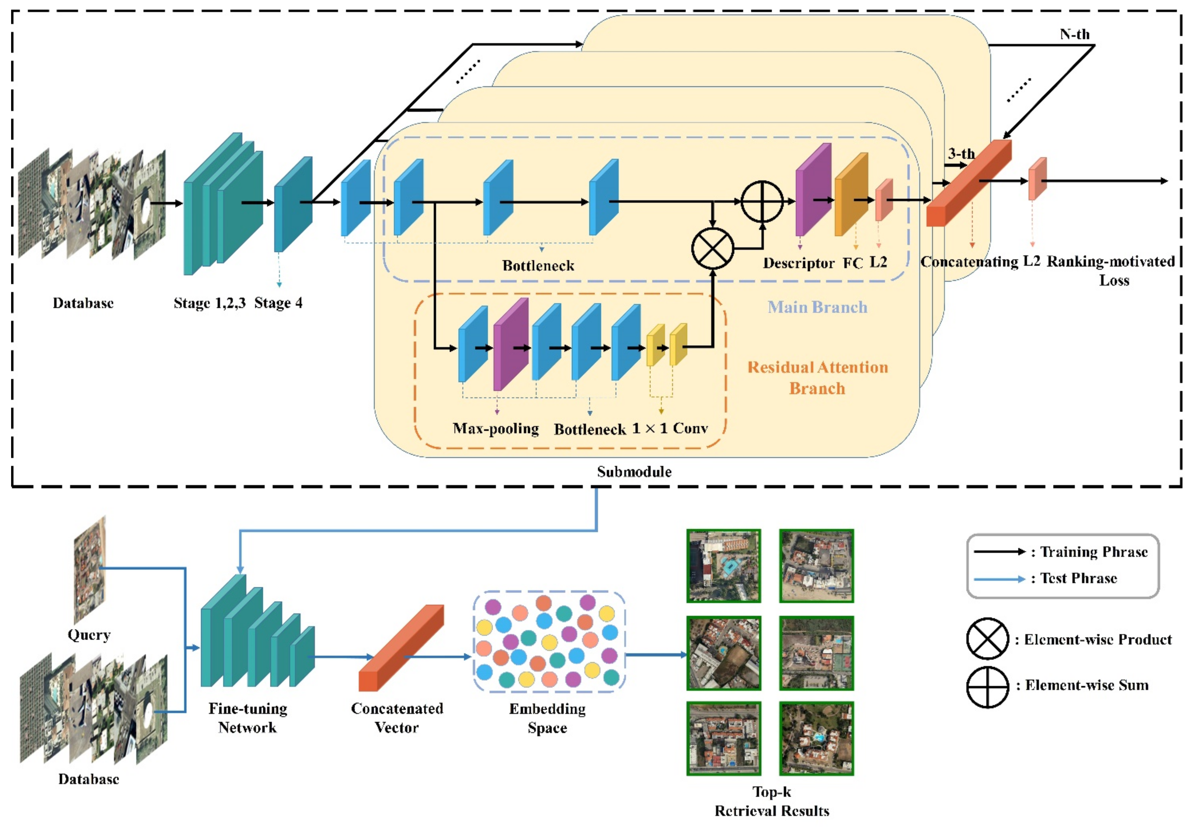
We propose a novel ensemble architecture of residual attention-based deep metric learning (EARA) for RSIR, illustrated in Figure 1. The bottleneck of ResNet is referred to as basic layers to construct the architecture. The proposed architecture consists of a ResNet backbone network and multiple submodules configured in two branches: As for the Main Branch, the individual descriptor is trained in an end-to-end manner with a ranking-motivated loss. In the Main Branch, Stages 1, 2, and 3 are the same as those in the ResNet50 and are composed of 3, 4, and 6 bottlenecks, respectively. The Residual Attention Branch is the soft attention mask and is added on Stage 4 of ResNet. The number of submodules n is determined by the dataset characteristics during the training phrase. Finally, submodules are merged to get the concatenated vectors by the proposed architecture.
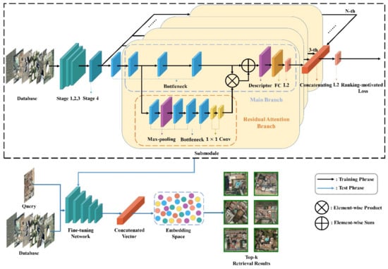
Figure 1.
The overall architecture of EARA. The upper part framed by black dashed box is the training process of the network, and the bottom is the testing process.
The retrieval process is described in Figure 1. First, the upper part framed by a black dashed box shows the network trained with a ranking-motivated loss. Then, the pretrained network (in black dashed box) is fine-tuned, which is denoted as the fine-tuning network in the test phase to complete the image retrieval task for more discriminative feature representations. Query image and the testing set would be input into the fine-tuned network, and the top K similar images would be returned.
3.1. Submodule
The submodule is composed of the Main Branch and Residual Attention Branch. With respect to the Main Branch, it is trained in an end-to-end manner to get global features of remote sensing images with the individual descriptor. The Residual Attention Branch added on the Main Branch is designed to extract more discriminative features and determine the subsequent weight calculations in a dynamic manner. Plus, the Residual Attention Branch can retain the information obtained by the Main Branch. The Residual Attention Branch in a submodule contains one residual attention in Stage 4 of ResNet50, and the distinguishability of the features extracted by it is basically the same as that of stacking multiple residual attentions. The descriptor ensemble further guarantees the distinguishability of semantic features of images. The most suitable position for adding a single Residual Attention Branch is Stage 4, where feature discriminability is the highest. The identity mapping of the Main Branch is combined with the soft attention mask in the Residual Attention Branch to construct the submodule. Two branches belonging to the submodule retain the original image information and rich semantic information (from the Residual Attention Branch) can enhance the performance. In addition, the online triplet mining was used, because it was more efficient, compared to the native triplet mining, in forming triplets (i.e., an anchor sample, a positive sample, and a negative sample) [19]. Based on the given anchor, the hard triplet mining strategy [24] is an exhaustively mining positive sample and negative sample to form a triplet in the mini-batch, in which the negative sample is most similar to the anchor among all negative samples, and then directly calculates the loss function online, which improves the mining efficiency and makes full use of the image information forms of more triples compared with the native triplet mining strategy.
3.1.1. Main Branch
In EARA, three influential pooling methods are utilized in the Main Branch of each submodule—namely, SPoC, MAC, and GeM—as descriptors. SPoC is a sum pooling method that aggregates local features to form a global feature. MAC is the maximum pool of downsampling images without losing image features as much as possible. GeM combines most of the parameters in the maximum pooling with the average pooling process, so as to maintain more information.
Let be the training set and the corresponding be the labeling set, where represents the th image whose class label is . We denote the number of classes is in , where . Let be the set of images in class , where the total number of images in class is .
Given an input image, we take the feature maps produced by the last convolutional layer as output of CNNs, which is of the form , where denotes the number of channels, represents the weight parameter, and represents the input to descriptors. We always assume ReLU activation is applied. Let be the set of activations for feature maps . Denoted by the th feature map of X, we apply the pooling process to produce a vector , where represents , so that the input image can be represented by the vector , and the corresponding descriptor is given by:
Set SPoC, MAC as , by taking , . As for GeM, denoted for the rest of the cases, there is a different pooling parameter for each feature map . In our experiments, the fixed parameter is employed for 3. Output feature vector from the th branch is generated by dimensionality reduction through the FC layer and normalization through the L2 normalization layer:
for , where is the weight of the th branches, and s, m, and g represent SPoC, MAC, and GeM, respectively.
The final feature vector is concatenated by , denoted as the output of the feature vector of all the Main Branches, and performs L2 normalization successively:
3.1.2. Residual Attention Branch
In RSIR, multiple types of attention are adopted to solve the problem of high inter-class similarities and intraclass differences resulting from the same spectra from different objects and the same object exhibiting different spectra in images and complex geographic locations. Since a single attention module can only modify the features of the model once, multiple types of attention modules are needed, leading to the increase of the model depth. Directly stacking attention modules in CNN architecture results in conspicuous performance degradation. On the one hand, the feature value is decreased by recurring dot production with a mask ranging from 0 to 1. On the other hand, a soft attention mask is likely to discard some key information extracted by deep network.
With the consideration of the above problems, the Residual Attention Branch is added onto the Main Branch to obtain the more discriminative features and maintain the original features of the images, which gives a boosted performance compared to the identity mapping. The soft attention mask is defined as a feature selector, which can enhance information-rich features. In EARA, we utilize mixed attention , channel attention , and spatial attention as the activation functions:
where denotes the mean value from the th channel and the standard deviation of the feature map from the th channel [30].
Therefore, output of the combination of the Residual Attention Branch and corresponding layers in the Main Branch are updated as:
where ranges from , denotes an element-wise product, the input is the features generated by CNNs different from the origin residual function , and the origin in residual learning is formulated as .
3.2. Loss Function
After merging all the submodules, concatenated vectors are obtained for the subsequent loss function calculations, and the corresponding algorithm is described in Algorithm 1.
| Algorithm 1: Merged submodules for our architecture |
| 1: Input: , 2: Output: 3: */forward propagation: 4: The submodule: 5: for i = 1 to n do 6: 7: In Residual Attention Branch: 8: 9: 10: 11: end for 12: for do j = 1 to L 13: 14: 15: end for |
| 16: Calculation of |
EARA can be extended with any typical ranking-motivated loss function like the N-pairs Loss [39], Proxy-NCA Loss [41], Lifted Struct Loss [21], and Batch Hard Triplet Loss [24]. The triplet loss with a hard batch mining strategy, which were verified to have excellent performances in remote sensing retrieval in Reference [24], were used as a quintessential example here. To exhaust all triplets on the mini-batch I, the hardest positive sample and negative sample within the mini-batch are employed to form a triplet to compute the loss, formulated as follows:
where represents the squared Euclidean distance between samples, represents the feature extractor parameterized by , and m denotes the margin between positive and negative sample.
4. Experiments
In this section, thorough experiments are conducted to evaluate the EARA performance in RSIR. First, ablation experiments are conducted to identify the effects of different activation functions in the Residual Attention Branch on the type and number of features, the descriptor of the Main Branch, and the ultimate loss function, respectively. Next, the retrieval performance of EARA is compared with the state-of-the-art DML-based ensemble methods on three benchmark remote sensing datasets, including UCMD, SIRI-WHU, and AID using three metrics: the overall retrieval accuracy (mAP), each category retrieval accuracy (mAP), and retrieval execution complexity (retrieval time and time used for model training).
4.1. Datasets
Experiments were conducted on three remote sensing benchmark datasets: UCMD, SIRI-WHU, and AID, among which, the number of images per category varies from 100 to 420, facilitating an understanding the influence of category quantity and the number of images per category on our architecture.
- UCMD: The UCMerced Land Use Database (UCMD) [31] is a land cover or land use dataset used as the RSIR benchmark dataset, which is a highly challenging dataset with some highly overlapping categories, such as the dense residential and intersection. It contains 21 classes, and each class has 100 images of 256 × 256 pixels with a spatial resolution of approximately 0.3 m. The images were downloaded from the United States Geological Survey (USGS) by the team at the University of California Merced from various US urban areas.
- SIRI-WHU: Google Image Dataset of SIRI-WHU [32] contains 2400 remote sensing images with a size of 200 × 200 pixels and a spatial resolution of 2 m. This dataset contains 12 geographic categories, and there are 200 images in each category. The number of images per category is twice than that in UCMD, while the number of categories is approximately same as UCMD, which would show the impact of the quantity per class on the discrimination of the features extracted by the architecture.
- AID: Aerial Image Dataset (AID) [33] is a dataset specifically designed for remote sensing image classification and retrieval tasks. It contains a total of 10,000 images divided into 30 semantic classes, such as commercial, dense residential, and viaduct. All the images have a size of 600 × 600 pixels in the RGB space, with a spatial resolution ranging from 8 to 0.5 m, and the number of each semantic class varies from 220 to 420 images. The number of images of AID is four times the size of UCMD and twice SIRI-WHU.
4.2. Configurations of Architecture
We performed the experiments on Ubuntu 16.04 with a single GTX 1080 Ti GPU and 2.10 GHz CPU. We implemented our method using Pytorch. To avoid attenuation induced by a deep network, ResNet-50 was selected as the baseline backbone. The Mean Average Precision (mAP) and Recall of the top-k (R@k) (k = 1, 2, 4, and 8) were utilized to evaluate the retrieval accuracy of EARA. FLOPs represent the complexity of EARA. An Adam [52] optimizer was used with a learning rate set at and scheduled by a step decay. A margin of m for triplet loss is set to 0.1 [36], and a temperature of τ for the SoftMax loss is set to 0.5 [37], with a batch size of 128, which are all empirical values.
Since the amount of data in UCMD, SIRI-WHU, and AID is enough for EARA learning, the train–test dividing strategy rather than data augmentation is adopted. The data-dividing ratio of training and testing data is set at 50%/50% for UCMD and, following, 80%/20% for SIRI-WHU and AID [17]. The experimental result is generally great [17] with the train–test dividing strategy for UCMD, SIRI-WHU, and AID. The same train–test dividing strategy is applied to other methods for fair comparisons. In the training phase, the input image is resized to 256 × 256, cropped randomly to 224 × 224, and then flipped randomly to the horizontal. In the testing phase, we only resize the image by the default input size of 224 × 224.
4.3. Ablation Experiments
The ablation experiments were conducted from three aspects, activation functions of the Residual Attention Branch, descriptors of the Main Branch, and loss function to analyze their respective effects on the entire architecture.
4.3.1. Activation Functions of Attention in Residual Attention Branch
Three activation functions are used here—namely, channel attention , spatial attention , and mixed attention . Channel attention performs L2 normalization on all feature maps in each spatial position to discard spatial information. Spatial attention ignores the information in all channel position by L2 normalization, which limits the spatial attention to the feature extraction stage, making it less explainable in other CNN layers. Mixed attention, combining the advantages of both, has less limitations and richer channel and spatial information. The experimental results on UCMD, SIRI-WHU, and AID, illustrated in Table 1, demonstrate that the performance of mixed attention outperforms the other two attention types.

Table 1.
mAP (%) for RSIR when three attention functions are used in the proposed architecture applied on UCMD, SIRI-WHU, and AID.
4.3.2. Impact of Type and Numbers of Descriptors on RSIR Performance
The type of descriptors on the Main Branch can be flexibly adapted to the corresponding network. In this experiment, we used the most advanced three pooling methods—namely, SPoC(S), MAC(M), GeM(G). Due to the structural characteristics of the convolutional network layer, the basic embedding sizes of the descriptor in RSIR are 256 and 512. In order to match the subsequent Residual Attention Branch, the embedding size of the descriptor would be the same as that of the Residual Attention Branch. Meantime, considering the concatenation of three types of descriptors (such as SGM), the descriptor dimension of each Main Branch is unified to 1536. We compared the seven configurations: S, M, G, SM, SG, MG, and SGM obtained by these three methods. As for S, M, and G, the single descriptor has 1536-dimensional embedding vectors. Except for S, M, and G, the rest of the configurations are composed of multiple descriptors with equal weights. For example, SM means to concatenate SPoC (to get a 768-dimensional vector) and MAC (to get a 768-dimensional vector) to get a feature vector with a dimension of 1536. Since the retrieval performance by using different kinds of descriptors is dependent on different datasets, we tested the seven configurations on UCMD, SIRI-WHU, and AID, respectively. As shown in Figure 2, in most cases, the method based on combined descriptors has a better performance compared to a single descriptor. Both the theoretical analysis and experiments suggest there are generally two kinds of errors in the feature extraction stage. The first is the variance of estimates generated in the finite neighborhood, and the second is the estimated mean deviation caused by the convolutional layer parameter error. SPoC is the sum pooling and can reduce the first error and, thus, maintain more image background information. GeM combines most of the parameters in the maximum pooling with the average pooling process, so as to reduce the second error. The best performance is obtained by the combination of SPoC ( single descriptor) and GeM (), set as SG. Figure 3b demonstrates the impact of three configurations (SG, S, and G) on the feature discrimination and retrieval performance. A denser distribution of dots of the same kind, a lesser intersection of dots of different classes, and the larger the interval, the better the clustering and retrieval performance. The architecture with configuration SG, which can extract the most discriminative features among those with configurations S and G, has the strongest ability to classify and retrieve data.
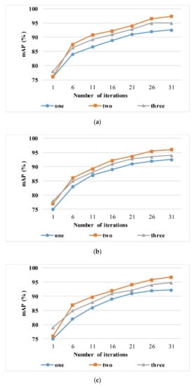
Figure 2.
The influence of numbers of descriptors on mAP. The evaluation is performed with our architecture on (a) UCMD, (b) SIRI-WHU, and (c) AID. The curve represents the evolution of mAP in the training iteration.

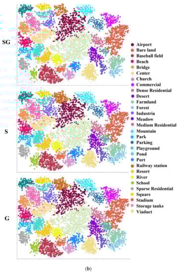
Figure 3.
The visualizations of feature discrimination. (a) The heatmap and evaluation are provided with configuration SG, S, and G on UCMD, SIRI-WHU, and AID. A more compact feature area means the feature is more discriminative. Each row corresponds to a test case: the query is shown in the first column, and the second to fourth columns are the visualization of the attention of the three configurations (SG, S, and G) of the query image. (b) The scatter plots are provided with configurations SG, S, and G on AID from top to bottom. Each color corresponds to each category of AID. A denser distribution of dots of the same color and a larger distance among dots of different colors indicate a better retrieval performance.
Table 2 shows the performance of single descriptors and combined multiple descriptors on the UCMD. Recall@1 of the SG is the highest among these configurations. The results demonstrated that the configuration SG not only has overall global information but also retains distinctive local regions. Generally speaking, a larger embedding dimension can lead to a better model performance. Figure 3a shows the feature discrimination of different pooling methods. The red parts indicate a strong contribution of identified features to improve the performance of RSIR. It illustrates that the configuration SG is helpful to extract discriminative features. Figure 3b demonstrates the impact of three configurations (SG, S, and G) on the feature discrimination and retrieval performance. A denser distribution of dots of the same kind, a lesser intersection of dots of different classes, and the larger the interval, the better the clustering and retrieval performance. The architecture with the configuration SG, which can extract the most discriminative features among those with the configuration S and G, has the strongest ability to classify and retrieve data.
Table 2.
Recall@1 (%) of individual descriptor and descriptors ensemble on UCMD, SIRI-WHU, and AID.
4.3.3. Comparison with SOTA Ranking-Motivated Losses
In this section, we compare the loss function in our architecture with the N-pairs Loss [39], Proxy-NCA Loss [41], Lifted Struct Loss [21], and Batch Hard Triplet Loss [24]. We denote the performance of the configuration SG as a baseline. The experiment results are shown in Table 3. The Batch Hard Triplet Loss performs best on the UCMD, SIRI-WHU, and AID in RSIR. This better performance should be attributed to the fact that the Batch Hard Triplet Loss method makes full use of valid triplets within each training mini-batch and has a fast convergence.
Table 3.
The evaluation results of mAP (%) and R@1 (%) on UCMD, SIRI-WHU, and AID compared with the other structure losses.
4.4. Comparative Experiments with SOTA Methods
To further evaluate the effectiveness and efficiency of our architecture, comparative experiments are conducted in overall retrieval accuracy (mAP), each category of retrieval accuracy (mAP), and retrieval execution complexity (retrieval time and time used for model training) among the EARA and four SOTA DML-based ensemble methods.
4.4.1. Comparison with Multiple DML-Based Ensemble Methods in RSIR
To show the performance of our architecture, we compared EARA with previous DML-based ensemble approaches in RSIR on the UCMD, SIRI-WHU, and AID in Table 4. We denote the excellent work provided by Sanakoyeu et al. [36] and the method proposed by Kim et al. [37] as DCES and ABE, respectively. As for ABE, we choose ABE-8 to finish the experiments, which has the best performance in RSIR [37]. The other two methods with outstanding contributions proposed by Opitz et al. [34,35] were recorded as BIER and A-BIER for convenience. To be fair, we did a ceteris paribus analysis, setting the embedding dimension as 1536 and selecting ResNet50 as the CNN backbone. Compared with the BIER, A-BIER, DCES, and ABE, the proposed architecture provides a significant improvement of 11.46%, 6.93%, 3.72%, and 0.72% in mAP and 17.46%, 11.35%, 10.32%, and 4.08% in R@1 on UCMD. Furthermore, the proposed architecture achieves a gain of 9.75% in mAP and 8.45% in R@1 on SIRI-WHU, which surpasses the recently published DCES and achieves a mAP of 96.81%, R@2 of 97.58%, and R@4 of 98.50%. As for AID, the improvement of our model gains 6.62%, 5.51%, and 4.89% in mAP, R@1, and R@2 compared with ABE. As can be seen from Table 4, our proposed architecture shows great performance in the field of RSIR.
Table 4.
Comparisons of the proposed architecture with state-of-the-art methods in RSIR using the UCMD, AID, and SIRI-WHU datasets (Recall@1, 2, 4, and 8 (%) and mAP (%)).
4.4.2. Comparison in Overall Results and Per-Class Results
To further analyze the effectiveness of our model, we present experiments on UCMD, SIRI-WHU, and AID for every geographic category in Table 5, Table 6 and Table 7, and the best results are highlighted in bold. The final retrieval results are shown in Figure 4, Figure 5 and Figure 6, respectively.
Table 5.
mAP (%) of 21 geographic categories in UCMD with various RSIR methods.
Table 6.
mAP (%) of 12 geographic categories in SIRI-WHU with various RSIR methods.
Table 7.
mAP (%) of 30 geographic categories in AID with various RSIR methods.
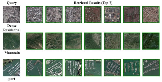
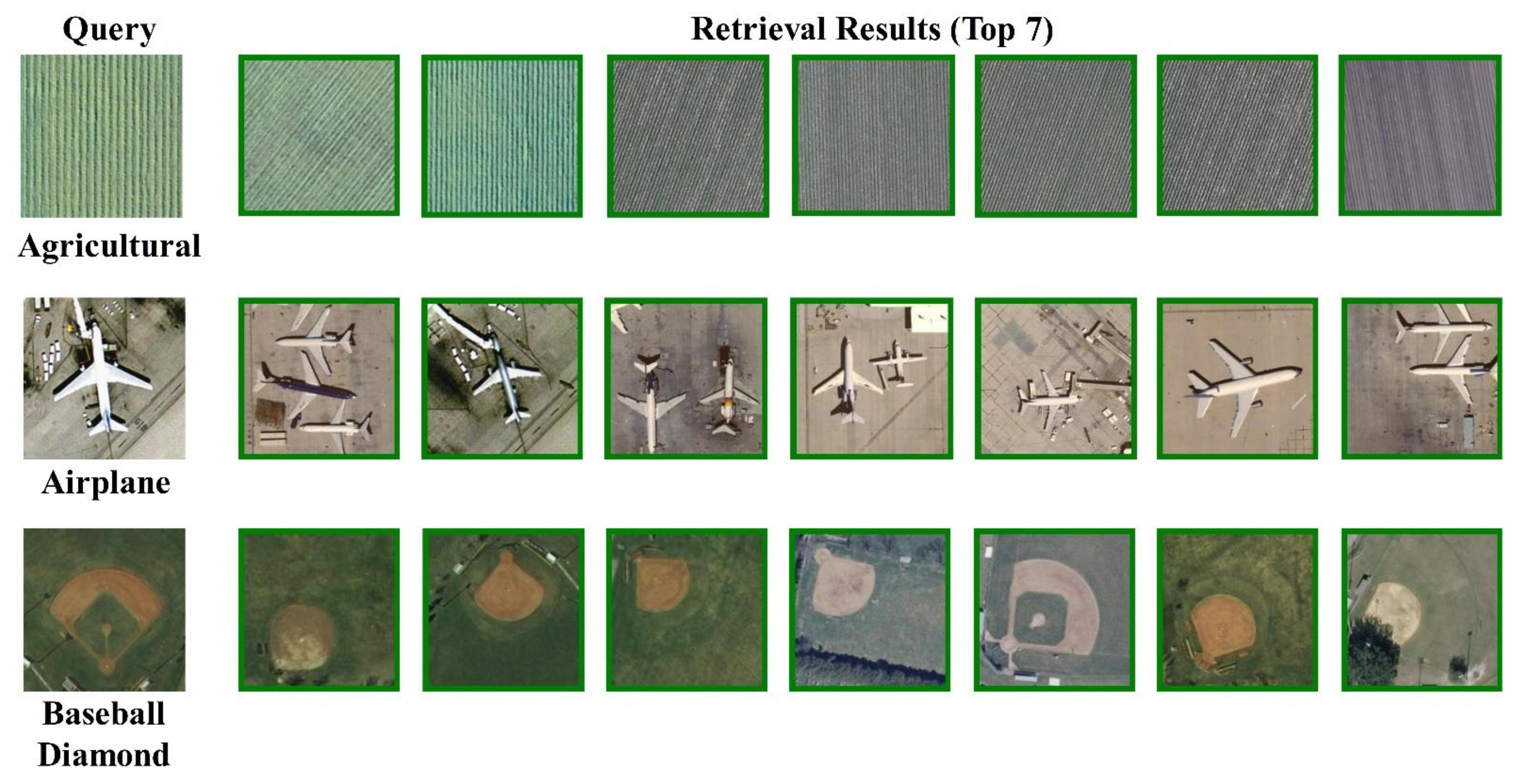
Figure 4.
Examples of the retrieval results on UCMD. Each row corresponds to a test case: the query is shown in the first column, and the second to fifth columns are the retrieval results ranked from 1 to 8. For each dataset, the first row represents the results derived from our method, and the second to sixth rows are the results from DCES, BIER, A-BIER, and ABE.
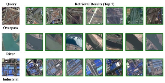
Figure 5.
Examples of the retrieval results on SIRI-WHU. Each row corresponds to a test case: the query is shown in the first column, and the second to fifth columns are the retrieval results ranked from 1 to 8. For each dataset, the first row represents the results derived from our method, and the second to sixth rows are the results from DCES, BIER, A-BIER, and ABE.

Figure 6.
Examples of the retrieval results on AID. Each row corresponds to a test case: the query is shown in the first column, and the second to fifth columns are the retrieval results ranked from 1 to 8. For each dataset, the first row represents the results derived from our method, and the second to sixth rows are the results from DCES, BIER, A-BIER, and ABE.
EARA gives the boosted retrieval performance for 15 out of 21 categories on UCMD, shown in Table 5. Compared to the state-of-the-art performance, EARA achieves an optimal performance in most categories. Specially, mAP of EARA outperforms that of BIER and A-BIER by 11.46% and 6.93% and obtained the improvement of 3.72% and 0.72% over DCES and ABE. EARA can achieve a better retrieval performance for images that contain rich spatial structure information. The reason might be that the configuration SG of EARA can preserve the spatial and channel information of the image as much as possible. This information makes the extracted features more discriminative, compared with that extracted from original configuration (such as S and G). However, the performance obtained by EARA on the other six categories is slightly inferior to that of ABE. The reason might be that the number of images contained in each category in UCMD is inadequate to train the network. Especially, the accuracy of the four SOTA methods was poor in retrieving categories, including “baseball diamond”, “building”, “harbor”, “intersection”, “mobile home park”, and “tennis court”. Comparatively, EARA outperforms the second-ranked ABE in retrieving “baseball diamond” and “buildings” by 2.23% and 5.81%, respectively. However, the performance obtained by EARA on the other six categories is slightly inferior to that of ABE. The reason might be that the number of images contained in each category in UCMD is inadequate and insufficient to obtain enough data to train the network.
Table 6 shows that our architecture achieves the state-of-the-art performance in all categories. EARA achieves a higher retrieval performance on SIRI-WHU than that of UCMD. Compared with the UCMD, the SIRI-WHU has a larger number of images with larger inter-class differences and, thus, can better evaluate EARA. Multiple types of attention are adopted by EARA to reduce the high inter-class similarities and intraclass differences, thus improving the RSIR performance. The average of mAP reaches up to 96.81%, with 10.59% higher than second-ranked ABE. The proposed architecture provides improvements in the retrieval accuracy compared with the existing results on the categories of “Harbor”, “Industrial”, “Overpass”, “Residential”, and “water” of 11.31% (from 87.12% to 98.43%), 12.61% (from 87.02% to 99.63%), 11.78% (from 83.25% to 95.03%), 12.07% (from 81.87% to 93.94%), and 12.07% (from 83.58% to 96.65%), respectively.
Table 7 shows that EARA improves the retrieval performance for most of categories on AID. As for the mAP of all categories, the value reaches 95.37% from 88.75% with 6.62% enhancement, which ranked . In general, our architecture outperforms the other four SOTA ensemble methods on AID, thanks to two reasons: First, descriptor ensemble and multiple types of attention in our architecture, maintaining rich spatial and channel information (such as intrinsic structure information), can reduce high inter-class similarities and intraclass differences resulting from the same spectra from different objects and the same object exhibiting different spectra in images. Second, AID contains more image categories and numbers, which is more suitable for data-driven EARA. The EARA performance on AID is much better than that on UCMD, which is reflected in the fact that EARA improves the retrieval indicators by 6.62–25.45% on AID compared to the other four methods, while on the UCMD dataset, it improves from 0.72% to 11.46%. Especially, EARA increases the mAP by 13.46% (from 83.67% to 97.13%) over ABE on “Sparse Residential”, 11.02% (from 83.94% to 94.96%) on “Dense Residential”, 10.63% (from 83.21% to 93.84%) on “Industria” and 10.47% (from 84.66% to 95.13%) on “Square”. EARA performs well in AID, except for two categories compared to ABE. DCES and ABE achieve the same excellent results on “Park” with 0.98% enhancement of that of EARA.
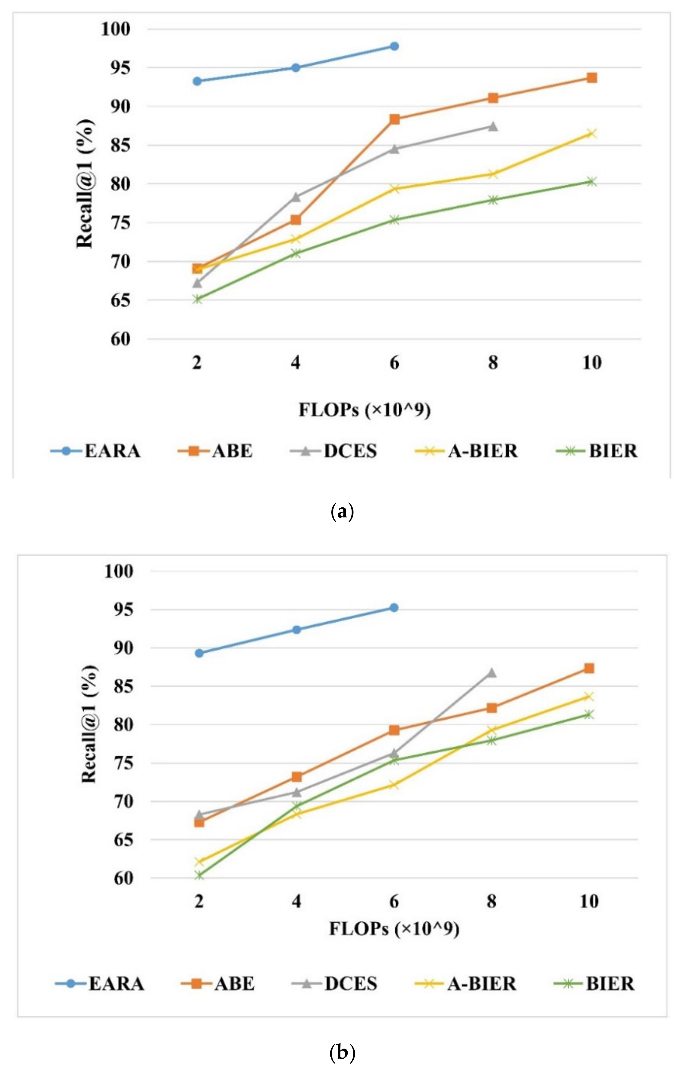
4.4.3. Comparison with DML-Based Ensemble Methods in Retrieval Execution Complexity
In comparison with the other ensemble methods, the retrieval execution complexity was also analyzed in terms of computational time cost and memory usage. First, we measure the time required for the retrieval process, including the time used for deep feature extraction (in minutes) and similarity metric computation (retrieval time). We set the embedding size of all methods to 512. The results on Table 8 demonstrate that our architecture needs much less time in retrieving the corresponding results compared with the other four methods. Even though the embedding size was set to 1536, the improvement on retrieval time is dramatically huge. Specifically, it takes about 10 milliseconds to extract deep features for each image with a size of 224 × 224, which is better than the previous fastest RSIR methods reported in Reference [52]. On UCMD, SIRI-WHU, and AID, the total time of training process only takes 25, 29, and 39 min, respectively. As shown in Figure 7, EARA outperforms the other ensemble methods in terms of retrieval execution complexity while ensuring retrieval accuracy. Second, we measured the retrieval execution complexity by using the metric FLOPs. Figure 7 shows that, when Recall@1 remains the same, the FLOPs of EARA on AID is only nearly one-fourth of A-BIER, two-thirds of BIER, and one-fifth of ABE. This reduction in computational time can be explained by the fact that other SOTA ensemble methods need individual training and test processes and the ensemble N number of learners with different descriptors requires quite a few numbers of GPUs. Besides, those methods require post-processing such as concatenation or normalization, which results in higher FLOPs and a longer computational time. In contrast, EARA needs only one GPU, and it omits the post-processing step via sharing a backbone. Therefore, EARA has remarkable efficiency in terms of the time costs and memory usage, especially for high-dimension embeddings.
Table 8.
Retrieval time (milliseconds) and time used for extracting image features (minutes) on AID with various RSIR methods.
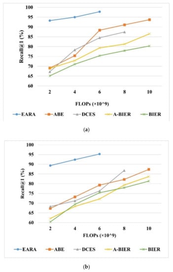
Figure 7.
Comparison of the proposed architecture with BIER, A-BIER, DCES, and ABE as evaluated by Recall@1 on (a) UCMD, (b) SIRI-WHU, (c) and AID. The overall embedding feature is 512.
5. Discussion
EARA shows relatively stable retrieval results despite the variations in time instance and shooting range, as shown in Figure 4, Figure 5 and Figure 6. The submodule, including the Main Branch and Residual Attention Branch, of EARA makes extracted features more discriminative. In addition, the descriptor ensemble method was adopted by EARA to decrease the high-computation complexity of similar metric algorithms in RSIR. Three factors affect the EARA performance: the type of the dataset, the number of images in the dataset, and the network structure.
When it comes to the dataset type and the number of images in the dataset, EARA can give more play to its advantages on datasets with more categories such as AID and SIRI-WHU. The better performance of EARA on AID and SIRI-WHU than on UCMD demonstrates that EARA is somewhat data-driven with no need for a large number of parameters to constraint learners, and EARA can benefit from large-scale datasets. With a large amount of data, EARA can fully learn the similarities and dissimilarities between the images. Nevertheless, great retrieval results on UCMD demonstrate that EARA also performs well on small datasets. The reason may be that ensemble descriptors and the addition of residual attention empower EARA to deeply explore the correlation between limited data and then to yield more distinguishable and comprehensive information of images. In the future, further refining of the loss function may expand the application of EARA to both large and small datasets.
With respect to the network structure, EARA improves the retrieval performance from the following aspects. First, the improvement of the network configuration, i.e., the addition of the Residual Attention Branch, maintains the global and discriminative features. In particular, the residual attention retains more structural feature information within the same class during sampling, which is beneficial for the subsequent calculation of similarity metrics. Second, the descriptor ensemble further encourages the diversity of the features without extra parameters to ease the time and memory burdens. Third, EARA dynamically weighs the feature vectors of the submodules to obtain the overall effect and can extract more discriminative features.
Moreover, EARA has superiority in retrieval execution complexity over other methods. The addition of residual attention avoids network attenuation induced by stacking many layers during feature extraction, speeds up the convergence, and reduces the high-computation complexity in terms of FLOPs and time cost. EARA adopts the online retrieval strategy for fine-tuning the pretrained network and makes the retrieval performance in line with a users’ standards. Different from other ensemble methods, EARA requires only one GPU, because it shares parameters without any postprocessing steps, and hence, it further reduces the training time and FLOPs, which are only 41% and 78% of the ABEs, respectively.
In general, EARA used a lower retrieval time on three remote sensing benchmark datasets in RSIR, compared with other DML-based methods. Consequently, EARA is beneficial to improve the retrieval efficiency of large-scale remote sensing images. EARA does not perform as well on small-scale datasets as it does on large-scale datasets. In future work, the loss function for small-scale datasets can be designed to further improve the retrieval performance. EARA is limited by images of insufficient spatial information and single channel information. The subsequent work may add some tricks (such as data augmentation) to solve this problem. Nevertheless, EARA is scalable in a variety of networks and loss functions, which offer widespread opportunities for EARA in many important application fields, such as aerial scene retrieval and environmental detection.
6. Conclusions
In this paper, we propose a novel residual attention-based ensemble architecture under a deep metric learning paradigm for RSIR. EARA boosts the RSIR performance owing to the following three aspects: the addition of residual attention, ensemble descriptors, and the scalability of network and loss function. First, the Residual Attention Branch is added onto the Main Branch to construct submodules to obtain more discriminative semantic features, preserve the complete global information, and avoid network attenuation. Moreover, the dynamic weight calculation dependent on the distinguishability of the extracted feature from the Residual Attention Branch can make full use of the extracted semantic information. Second, multiple descriptors of the Main Branch in submodules are aggregated into feature vectors to achieve complete global and distinctive image information. Third, compared to the SOTA methods such as BIER [34], A-BIER [35], DCES [36], ABE [37], and EARA exhibited an improvement of 15.45%, 13.04%, 10.31%, and 6.62% in mAP on AID. In addition, the retrieval time and FLOPs to implement EARA are reduced by nearly 20% and 8% of ABE on AID.
The results suggest the effectiveness of the proposed architecture in RSIR in terms of the retrieval accuracy and execution complexity. Thorough experiments on three remote sensing benchmark datasets that include UCMD, SIRI-WHU, and AID demonstrate that EARA achieves a better performance with a reduced time cost and fewer parameters, compared with four SOTA DML-based ensemble methods. EARA offers widespread opportunities in many important application fields, such as aerial scene retrieval and environmental detection.
Author Contributions
Conceptualization, Q.C. and D.G.; methodology, Q.C. and D.G.; software, D.G.; validation, Q.C. and D.G.; formal analysis, P.F.; investigation, D.G.; resources, Q.C.; data curation, D.G.; visualization, H.H. and Y.Z.; writing—original draft preparation, D.G.; writing—review and editing, Q.C. and P.F.; and funding acquisition, Q.C. All authors have read and agreed to the published version of the manuscript.
Funding
The work of this paper was supported by the National Key R&D Program of China (2018YFB0505401), National Natural Science Foundation of China (No. 41771452), and Director Fund of Institute of Remote Sensing and Digital Earth (Y5SJ1500CX).
Institutional Review Board Statement
Not applicable.
Informed Consent Statement
Not applicable.
Data Availability Statement
Not applicable.
Acknowledgments
The authors would like to thank reviewers for reviewing this paper and providing important feedback throughout its development.
Conflicts of Interest
The authors declare no conflict of interest. The funders had no role in the design of the study; in the collection, analyses, or interpretation of the data; in the writing of the manuscript; or in the decision to publish the results.
References
- Peijun, D.U.; Yunhao, C.; Hong, T.; Tao, F. Study on Content-Based Remote Sensing Image Retrieval. In Proceedings of the 2005 IEEE International Geoscience and Remote Sensing Symposium, IGARSS’05, Seoul, Korea, 29 July 2005; Volume 2, p. 4. [Google Scholar]
- Özkan, S.; Ateş, T.; Tola, E.; Soysal, M.; Esen, E. Performance Analysis of State-of-the-Art Representation Methods for Geographical Image Retrieval and Categorization. IEEE Geosci. Remote Sens. Lett. 2014, 11, 1996–2000. [Google Scholar] [CrossRef]
- Li, D.; Tian, Y. Survey and Experimental Study on Metric Learning Methods. Neural Netw. 2018, 105, 447–462. [Google Scholar] [CrossRef] [PubMed]
- Fernandez-Beltran, R.; Latorre-Carmona, P.; Pla, F. Single-Frame Super-Resolution in Remote Sensing: A Practical Overview. Int. J. Remote Sens. 2017, 38, 314–354. [Google Scholar] [CrossRef]
- Zhang, B.; Chen, Z.; Peng, D.; Benediktsson, J.A.; Liu, B.; Zou, L.; Li, J.; Plaza, A. Remotely Sensed Big Data: Evolution in Model Development for Information Extraction [Point of View]. Proc. IEEE 2019, 107, 2294–2301. [Google Scholar] [CrossRef]
- Yang, Y.; Newsam, S. Geographic Image Retrieval Using Local Invariant Features. IEEE Trans. Geosci. Remote Sens. 2012, 51, 818–832. [Google Scholar] [CrossRef]
- Li, E.; Du, P.; Samat, A.; Meng, Y.; Che, M. Mid-Level Feature Representation via Sparse Autoencoder for Remotely Sensed Scene Classification. IEEE J. Sel. Top. Appl. Earth Obs. Remote Sens. 2016, 10, 1068–1081. [Google Scholar] [CrossRef]
- Chen, Y.; Jiang, H.; Li, C.; Jia, X.; Ghamisi, P. Deep Feature Extraction and Classification of Hyperspectral Images Based on Convolutional Neural Networks. IEEE Trans. Geosci. Remote Sens. 2016, 54, 6232–6251. [Google Scholar] [CrossRef] [Green Version]
- Manjunath, B.S.; Ma, W.-Y. Texture Features for Browsing and Retrieval of Image Data. IEEE Trans. Pattern Anal. Mach. Intell. 1996, 18, 837–842. [Google Scholar] [CrossRef] [Green Version]
- Bretschneider, T.; Cavet, R.; Kao, O. Retrieval of Remotely Sensed Imagery Using Spectral Information Content. In Proceedings of the IEEE International Geoscience and Remote Sensing Symposium, Toronto, ON, Canada, 24–28 June 2002; Volume 4, pp. 2253–2255. [Google Scholar]
- Bratasanu, D.; Nedelcu, I.; Datcu, M. Bridging the Semantic Gap for Satellite Image Annotation and Automatic Mapping Applications. IEEE J. Sel. Top. Appl. Earth Obs. Remote Sens. 2010, 4, 193–204. [Google Scholar] [CrossRef] [Green Version]
- Ma, Y.; Wu, H.; Wang, L.; Huang, B.; Ranjan, R.; Zomaya, A.; Jie, W. Remote Sensing Big Data Computing: Challenges and Opportunities. Future Gener. Comput. Syst. 2015, 51, 47–60. [Google Scholar] [CrossRef] [Green Version]
- Li, Y.; Zhang, Y.; Tao, C.; Zhu, H. Content-Based High-Resolution Remote Sensing Image Retrieval via Unsupervised Feature Learning and Collaborative Affinity Metric Fusion. Remote Sens. 2016, 8, 709. [Google Scholar] [CrossRef] [Green Version]
- Ge, Y.; Jiang, S.; Xu, Q.; Jiang, C.; Ye, F. Exploiting Representations from Pre-Trained Convolutional Neural Networks for High-Resolution Remote Sensing Image Retrieval. Multimed. Tools Appl. 2018, 77, 17489–17515. [Google Scholar] [CrossRef]
- Pires de Lima, R.; Marfurt, K. Convolutional Neural Network for Remote-Sensing Scene Classification: Transfer Learning Analysis. Remote Sens. 2020, 12, 86. [Google Scholar] [CrossRef] [Green Version]
- Yang, L.; Jin, R. Distance Metric Learning: A Comprehensive Survey. Mich. State Univ. 2006, 2, 4. [Google Scholar]
- Ye, F.; Xiao, H.; Zhao, X.; Dong, M.; Luo, W.; Min, W. Remote Sensing Image Retrieval Using Convolutional Neural Network Features and Weighted Distance. IEEE Geosci. Remote Sens. Lett. 2018, 15, 1535–1539. [Google Scholar] [CrossRef]
- Hu, J.; Lu, J.; Tan, Y.-P. Deep Transfer Metric Learning. In Proceedings of the IEEE Conference on Computer Vision and Pattern Recognition, Boston, MA, USA, 7–12 June 2015; pp. 325–333. [Google Scholar]
- Schroff, F.; Kalenichenko, D.; Philbin, J. Facenet: A Unified Embedding for Face Recognition and Clustering. In Proceedings of the IEEE Conference on Computer Vision and Pattern Recognition, Boston, MA, USA, 7–12 June 2015; pp. 815–823. [Google Scholar]
- Chopra, S.; Hadsell, R.; LeCun, Y. Learning a Similarity Metric Discriminatively, with Application to Face Verification. In Proceedings of the 2005 IEEE Computer Society Conference on Computer Vision and Pattern Recognition (CVPR’05), Boston, MA, USA, 7–12 June 2015; Volume 1, pp. 539–546. [Google Scholar]
- Oh Song, H.; Xiang, Y.; Jegelka, S.; Savarese, S. Deep Metric Learning via Lifted Structured Feature Embedding. In Proceedings of the IEEE Conference on Computer Vision and Pattern Recognition, Las Vegas, NV, USA, 27–30 June 2016; pp. 4004–4012. [Google Scholar]
- Cheng, G.; Yang, C.; Yao, X.; Guo, L.; Han, J. When Deep Learning Meets Metric Learning: Remote Sensing Image Scene Classification via Learning Discriminative CNNs. IEEE Trans. Geosci. Remote Sens. 2018, 56, 2811–2821. [Google Scholar] [CrossRef]
- Roy, S.; Sangineto, E.; Demir, B.; Sebe, N. Deep Metric and Hash-Code Learning for Content-Based Retrieval of Remote Sensing Images. In Proceedings of the IGARSS 2018—2018 IEEE International Geoscience and Remote Sensing Symposium, Valencia, Spain, 22–27 July 2018; pp. 4539–4542. [Google Scholar]
- Cao, R.; Zhang, Q.; Zhu, J.; Li, Q.; Qiu, G. Enhancing Remote Sensing Image Retrieval with Triplet Deep Metric Learning Network. arXiv 2019, arXiv:1902.05818. [Google Scholar]
- Hadsell, R.; Chopra, S.; LeCun, Y. Dimensionality Reduction by Learning an Invariant Mapping. In Proceedings of the 2006 IEEE Computer Society Conference on Computer Vision and Pattern Recognition (CVPR’06), New York, NY, USA, 17–22 June 2006; Volume 2, pp. 1735–1742. [Google Scholar]
- Law, M.T.; Thome, N.; Cord, M. Quadruplet-Wise Image Similarity Learning. In Proceedings of the IEEE International Conference on Computer Vision, Sydney, NSW, Australia, 1–8 December 2013; pp. 249–256. [Google Scholar]
- Liu, P.; Gou, G.; Shan, X.; Tao, D.; Zhou, Q. Global Optimal Structured Embedding Learning for Remote Sensing Image Retrieval. Sensors 2020, 20, 291. [Google Scholar] [CrossRef] [Green Version]
- Zhao, H.; Yuan, L.; Zhao, H. Similarity Retention Loss (SRL) Based on Deep Metric Learning for Remote Sensing Image Retrieval. ISPRS Int. J. Geo Inf. 2020, 9, 61. [Google Scholar] [CrossRef] [Green Version]
- Chi, M.; Plaza, A.; Benediktsson, J.A.; Sun, Z.; Shen, J.; Zhu, Y. Big Data for Remote Sensing: Challenges and Opportunities. Proc. IEEE 2016, 104, 2207–2219. [Google Scholar] [CrossRef]
- Wang, F.; Jiang, M.; Qian, C.; Yang, S.; Li, C.; Zhang, H.; Wang, X.; Tang, X. Residual Attention Network for Image Classification. In Proceedings of the IEEE Conference on Computer Vision and Pattern Recognition, Honolulu, HI, USA, 21–26 July 2017; pp. 3156–3164. [Google Scholar]
- Yang, Y.; Newsam, S. Bag-of-Visual-Words and Spatial Extensions for Land-Use Classification. In Proceedings of the 18th SIGSPATIAL International Conference on Advances in Geographic Information Systems, San Jose, CA, USA, 2–5 November 2010; pp. 270–279. [Google Scholar]
- Zhu, Q.; Zhong, Y.; Zhao, B.; Xia, G.-S.; Zhang, L. Bag-of-Visual-Words Scene Classifier with Local and Global Features for High Spatial Resolution Remote Sensing Imagery. IEEE Geosci. Remote Sens. Lett. 2016, 13, 747–751. [Google Scholar] [CrossRef]
- Xia, G.-S.; Hu, J.; Hu, F.; Shi, B.; Bai, X.; Zhong, Y.; Zhang, L.; Lu, X. AID: A Benchmark Data Set for Performance Evaluation of Aerial Scene Classification. IEEE Trans. Geosci. Remote Sens. 2017, 55, 3965–3981. [Google Scholar] [CrossRef] [Green Version]
- Opitz, M.; Possegger, H.; Bischof, H. Efficient Model Averaging for Deep Neural Networks. In Proceedings of the Asian Conference on Computer Vision, Taipei, Taiwan, 20–24 November 2016; pp. 205–220. [Google Scholar]
- Opitz, M.; Waltner, G.; Possegger, H.; Bischof, H. Deep Metric Learning with Bier: Boosting Independent Embeddings Robustly. IEEE Trans. Pattern Anal. Mach. Intell. 2018, 42, 276–290. [Google Scholar] [CrossRef] [Green Version]
- Sanakoyeu, A.; Tschernezki, V.; Buchler, U.; Ommer, B. Divide and Conquer the Embedding Space for Metric Learning. In Proceedings of the IEEE/CVF Conference on Computer Vision and Pattern Recognition, Long Beach, CA, USA, 15–20 June 2019; pp. 471–480. [Google Scholar]
- Kim, W.; Goyal, B.; Chawla, K.; Lee, J.; Kwon, K. Attention-Based Ensemble for Deep Metric Learning. In Proceedings of the European Conference on Computer Vision (ECCV), Munich, Germany, 8–14 September 2018; pp. 736–751. [Google Scholar]
- Ba, J.; Mnih, V.; Kavukcuoglu, K. Multiple Object Recognition with Visual Attention. arXiv 2014, arXiv:1412.7755. [Google Scholar]
- Sohn, K. Improved Deep Metric Learning with Multi-Class n-Pair Loss Objective. In Proceedings of the Advances in Neural Information Processing Systems, Barcelona, Spain, 5–10 December 2016; pp. 1857–1865. [Google Scholar]
- Kim, S.; Seo, M.; Laptev, I.; Cho, M.; Kwak, S. Deep Metric Learning beyond Binary Supervision. In Proceedings of the IEEE/CVF Conference on Computer Vision and Pattern Recognition, Long Beach, CA, USA, 15–20 June 2019; pp. 2288–2297. [Google Scholar]
- Movshovitz-Attias, Y.; Toshev, A.; Leung, T.K.; Ioffe, S.; Singh, S. No Fuss Distance Metric Learning Using Proxies. In Proceedings of the IEEE International Conference on Computer Vision, Venice, Italy, 29 October 2017; pp. 360–368. [Google Scholar]
- Fan, L.; Zhao, H.; Zhao, H.; Liu, P.; Hu, H. Distribution Structure Learning Loss (DSLL) Based on Deep Metric Learning for Image Retrieval. Entropy 2019, 21, 1121. [Google Scholar] [CrossRef] [Green Version]
- Sudha, S.K.; Aji, S. A Review on Recent Advances in Remote Sensing Image Retrieval Techniques. J. Indian Soc. Remote Sens. 2019, 47, 2129–2139. [Google Scholar] [CrossRef]
- Zhu, S.; Dong, X.; Su, H. Binary Ensemble Neural Network: More Bits per Network or More Networks per Bit? In Proceedings of the IEEE/CVF Conference on Computer Vision and Pattern Recognition, Long Beach, CA, USA, 15–20 June 2019; pp. 4923–4932. [Google Scholar]
- Lin, Z.; Yang, Z.; Huang, F.; Chen, J. Regional Maximum Activations of Convolutions with Attention for Cross-Domain Beauty and Personal Care Product Retrieval. In Proceedings of the 26th ACM international conference on Multimedia, Seoul, Korea, 22–26 October 2018; pp. 2073–2077. [Google Scholar]
- Mnih, V.; Heess, N.; Graves, A. Recurrent Models of Visual Attention. In Proceedings of the Advances in Neural Information Processing Systems, Montreal, QC, Canada, 8–13 December 2014; pp. 2204–2212. [Google Scholar]
- Sermanet, P.; Frome, A.; Real, E. Attention for Fine-Grained Categorization. arXiv 2014, arXiv:1412.7054. [Google Scholar]
- Zhao, B.; Wu, X.; Feng, J.; Peng, Q.; Yan, S. Diversified Visual Attention Networks for Fine-Grained Object Classification. IEEE Trans. Multimed. 2017, 19, 1245–1256. [Google Scholar] [CrossRef] [Green Version]
- Jaderberg, M.; Simonyan, K.; Zisserman, A. Spatial Transformer Networks. Adv. Neural Inf. Process. Syst. 2015, 28, 2017–2025. [Google Scholar]
- Chen, L.-C.; Yang, Y.; Wang, J.; Xu, W.; Yuille, A.L. Attention to Scale: Scale-Aware Semantic Image Segmentation. In Proceedings of the IEEE Conference on Computer Vision and Pattern Recognition, Las Vegas, NV, USA, 27–30 June 2016; pp. 3640–3649. [Google Scholar]
- Sumbul, G.; Demir, B. A Novel Multi-Attention Driven System for Multi-Label Remote Sensing Image Classification. In Proceedings of the IGARSS 2019—2019 IEEE International Geoscience and Remote Sensing Symposium, Yokohama, Japan, 28 July–2 August 2019; pp. 5726–5729. [Google Scholar]
- Kingma, D.P.; Ba, J. Adam: A Method for Stochastic Optimization. arXiv 2014, arXiv:1412.6980. [Google Scholar]


Publisher’s Note: MDPI stays neutral with regard to jurisdictional claims in published maps and institutional affiliations. |
© 2021 by the authors. Licensee MDPI, Basel, Switzerland. This article is an open access article distributed under the terms and conditions of the Creative Commons Attribution (CC BY) license (https://creativecommons.org/licenses/by/4.0/).