Article

Variations in the Effects of Landscape Patterns on the Urban Thermal Environment during Rapid Urbanization (1990–2020) in Megacities

1
Institute of Geographic Sciences and Natural Resources Research, Chinese Academy of Sciences, Beijing 100101, China
2
College of Resources and Environment, University of Chinese Academy of Sciences, Beijing 100049, China
3
School of Environmental Science and Engineering, Tianjin University, Tianjin 300354, China
4
State Key Laboratory of Urban and Regional Ecology, Research Centre for Eco-Environmental Sciences, Chinese Academy of Sciences, Beijing 100085, China
5
Department of Urban Planning and Design, The University of Hong Kong, Pokfulam, Hong Kong, China
*
Author to whom correspondence should be addressed.
Remote Sens. 2021, 13(17), 3415; https://doi.org/10.3390/rs13173415
Submission received: 2 July 2021 / Revised: 18 August 2021 / Accepted: 19 August 2021 / Published: 27 August 2021

Abstract

:
Deterioration of the urban thermal environment, especially in megacities with intensive populations and high densities of impervious surfaces, is a global issue resulting from rapid urbanization. The effects of landscape patterns on the urban thermal environment within a single area or single period have been well documented. Few studies, however, have explored whether the effects can be adapted to various cities at different urbanization stages. This paper investigated the variations of these effects in the five largest and highly urbanized megacities of China from 1990 to 2020 using various geospatial approaches, including concentric buffer analysis, correlation analysis, and hierarchical ridge regression models. The results indicated that the effects of landscape patterns on the urban thermal environment were greatly variable at different urbanization stages. Although landscape composition was more important than landscape configuration in determining the urban thermal environment, the standard coefficients of composition metrics continuously decreased from 1990 to 2020. However, configuration metrics, such as patch density, edge density, and shape complexity, could affect the land surface temperature (LST) to a larger extent at the highly urbanized stage. The urbanization process could also affect the cooling effect of urban green space. At the initial stage of rapid urban expansion in approximately 2000, urban green space explained the most variation in LST, with a value as high as 10%. To maximize the cooling effect, the spatial arrangement of urban green space should be highlighted in the region that was 10–15 km from the city center, where the mean LST experienced a significant decline. These results may provide deeper insights into improving the urban thermal environment by targeted strategies in optimizing landscape patterns for areas at different urbanization stages.

1. Introduction

A megacity is generally considered a metropolitan area with a total population of more than 10 million [1]. It is estimated that there will be 43 megacities in the world by 2030 [2]. Approximately 55.7% of the population lives in urban areas [3], and this proportion is expected to increase to 70% by 2050 [2]. The most recent advances in Geographic Information Systems (GIS) provided us with substantial geospatial technologies, such as quantitative measurement of urban shape and monitoring cities in near real-time by drone, to address environmental disturbances and promote urban sustainable development during rapid urbanization [4,5]. China, as a developing country, has undergone large and continuous demographic migration from rural areas to urban areas [6]. Land cover change caused by urbanization is occurring at an unprecedented rate and results in changes in the structure and function of urban ecosystems [7,8]. As an important part of the urban eco-environment, the urban thermal environment is greatly affected by rapid urbanization, especially in megacities [9]. A well-documented consequence of the urban thermal environment change is the formation of urban heat island (UHI), referring to the phenomenon that the atmospheric and surface temperatures in urban areas are higher than those in the surrounding rural areas [10]. The urban thermal environment has a profound effect on the local climate, human settlement, energy consumption, biodiversity, and ecosystem functions [11,12,13,14]. On the one hand, continuous high temperatures will decrease the comfort of urban dwellers, which may cause greater health risks [15,16]. On the other hand, excess heat will greatly increase the energy consumption for building refrigeration, leading to economic burdens on urban development [17]. Urban warming in hot climates exerts heat stress on organisms and may thus reduce biodiversity and affect ecosystem functions [18]. Therefore, it is of special importance to investigate the factors that affect the urban thermal environment.
Many studies have shown that there is a significant relationship between the urban thermal environment and landscape patterns, which include composition and configuration [19,20]. For example, vegetation is replaced by impervious surfaces such as asphalt and cement, which represents a compositional change. The fragmentation of natural landscapes increases because of land cover change, which represents a configuration change. Both aspects result in radiation energy changes and provide an energy basis for the formation of UHI [21]. Urban thermal environment problems caused by landscape pattern changes have attracted widespread attention [10,22,23,24,25]. Land surface temperature (LST), which has continuous spatial coverage, has been an important parameter in manifesting the urban thermal environment in recent decades [26]. A series of studies have been carried out to investigate the effects of landscape patterns on the urban thermal environment using remotely sensed LST data. The results indicated that anthropogenic land cover types such as asphalt-paved areas and building areas play an important role in increasing LST, while natural land cover types such as green space, forests, and water bodies can mitigate high temperatures even in urban central areas [27,28,29]. There is a strong positive correlation between LST and the density of impervious land surfaces, which are generally accepted as the main driving force of temperature increases [30,31,32]. In contrast, urban green space has cooling effects on the urban thermal environment. Evidence reported in the reviewed papers showed that landscape configuration, including the spatial characteristics of individual landscape patches and the relationships among multiple areas, can also affect the urban thermal environment [7,33,34,35].
It is worth noting that the effects of landscape composition and configuration on the urban thermal environment are greatly variable due to the differences in the locations [36,37], the city size [38], and the urban development stage of the study areas [37]. Estoque et al. [39] examined the relationship between urban LST and the spatial patterns of impervious surfaces and urban green space in the three megacity areas of Manila, Jakarta, and Bangkok in Southeast Asia. The results showed that the correlation between the mean LST and landscape composition fluctuated across the three areas, in which the correlation coefficient of Jakarta (0.062) was larger than those of the other two areas (0.044 and 0.048). In Turin, Italy, urban LST significantly increased by 4.0°C, where the high impervious land surface increased by 10% in core areas [40]; however, for every one percent increase in impervious land surface in Hanoi, Vietnam, the mean LST will increase by approximately 0.75–1.08°C [41], and a 7.69% decrease in impervious surface density in Beijing was equivalent to a 1.1 °C decline in mean LST [42]. While landscape composition is much more important than configuration, landscape configuration cannot be neglected. Chen et al. [26] reported that the landscape shape index and mean gyration index, which were calculated by Landsat images acquired in 2002, can explain approximately 12% of the mean LST by statistical analysis in Beijing. However, even in the same study area, Peng et al. [43] reached different conclusions using Landsat images acquired in 2009. The correlation results showed that the landscape shape index could explain approximately 35% of urban LST, and the Pearson correlation coefficients of the shape index and fragmentation index with LST were 0.594 and 0.510, respectively. However, a study carried out in Baltimore using the same method showed that the Pearson correlation coefficients between LST and these two indexes were −0.30 and 0.31, respectively [44]. Being limited to a relative-narrow spatiotemporal range (the single city or single year), these studies mainly focused on the effects of landscape patterns on UHI intensity. These results suggested that the same landscape metric might play different roles and that some even showed contrary effects on the urban thermal environment. Few studies, however, have explored the variations in these effects using multiple thermal images for different years in different urban areas, particularly in megacities of China.
Taking five megacities (Beijing, Tianjin, Shanghai, Guangzhou, and Shenzhen), which are the core cities of the three most developed urban agglomerations in China [45], as the study areas, this study sought to: (1) examine the effects of landscape patterns on the urban thermal environment in the study areas, (2) and further investigated the variations in the effects from 1990 to 2020 across different urbanization stages. As the home of more than 10 million people, each of these five cities has experienced rapid urbanization and presented intensive UHI [46,47,48,49,50]. Landsat series data and various geospatial methods, including spatial metric-based approaches, land-use dynamic changes, and hierarchical ridge regression models, were used to facilitate the research. The results from this study can provide urban planners with deep insights into how to improve the urban thermal environment through targeted urban green space management and impervious surface design at specific urbanization stages.

2. Materials and Methods

2.1. Study Areas

The five largest megacities in China, Beijing, Tianjin, Shanghai, Guangzhou, and Shenzhen, are illustrated in Figure 1. Among them, Beijing and Tianjin are located in the Beijing-Tianjin-Hebei urban agglomerations, Shanghai is located in the Yangtze River Delta, and Guangzhou and Shenzhen are located in the Pearl River Delta. These megacities are similar in that they have dense and numerous populations, rapid urbanization, large GDP, and an intensive UHI effect. However, there are still significant differences among them in urban climate conditions, urbanization processes, and landscape patterns. Beijing and Tianjin, both situated in the northern part of the North China Plain, have a hot and humid summer because of the East China monsoon. Shanghai, as an economic center in China, is situated in the estuary of the Yangtze River, in which the humid subtropical climate is obvious in summer. Guangzhou and Shenzhen, located in coastal regions, are wet, with high temperatures in summer influenced by the subtropical monsoon climate.
The city cores of each megacity determined by the administrative boundary were selected as the study areas for two main reasons. On the one hand, the city cores covered most parts of the urban extent and presented typical UHI effects. On the other hand, the study areas can be covered by a single swath of satellite images to avoid the uncertainties caused by mosaicking two or more images. The landscapes of the five megacities included urban built-up lands, green space, and water bodies. However, the landscape patterns varied with different modes of urban expansion. Beijing and Shanghai had a prominent ring pattern and expanded in all directions due to the strong attractiveness of urban central areas. In contrast, Tianjin, Guangzhou, and Shenzhen, which are all coastal cities, showed ribbon patterns in the north-south (Guangzhou) or east-west (Tianjin and Shenzhen) directions due to terrain constraints. The Digital Elevation Model (DEM) with 30-m spatial resolution of five megacities were shown in Figure A1. In most cases, the central areas of cities are flat, while mountains and hills were basically located outside the study areas.

2.2. Data Source and Pre-Processing

To acquire cloud-free Landsat images with highly clear atmospheric conditions derived from three sensors, Landsat 5 TM6, Landsat 7 ETM+6, and Landsat 8 TIRSI, in different study periods, the image acquisition dates ranging from July to September were not strictly limited in the initial year of each decade, of which a deviation of two years was acceptable (Table 1). Thermal images of Shenzhen in the summer seasons from 2018 to 2020 were covered by large amounts of clouds; hence, the LST of Shenzhen was retrieved in approximately 1990, 2000, and 2010, excluding 2020. Each swath of the Landsat image covered the whole area of a single megacity. This study collected the meteorological data of the image acquisition date to assure that the satellite images were both cloud-clean and with similar weather conditions. From the acquired meteorological data (Table A1), the differences among the five megacities were not obvious, especially in the aspect of maximum temperature. Therefore, selected Landsat images, which were used to retrieve land surface temperature, had similar weather characteristics. The satellite images were composited by the method of standard false-color composition with Bands 2, 3, and 4 (Figure 1). Then, the false-color images were classified into four land cover categories, namely, impervious surface, urban green space, water body, and other.

2.3. LST Retrieval

For LST retrieval, the procedure suggested by Wang et al. [51] was applied. In this study, the emissivity-corrected LST was calculated as follows:
T s = c 2 / λ ln ( c 1 λ 5 B ( T s ) + 1 )
with
B ( T s ) w = a 0 + a 1 w + ( a 2 + a 3 w + a 4 w 2 ) 1 ε + ( a 5 + a 6 w + a 7 w 2 ) 1 ε L s e n
where Ts represents LST, λ represents the effective wavelength (11.457 μm, 11.269 μm, 10.904 μm for Landsat 5 TM6, Landsat 7 ETM+6, Landsat 8 TIRSI, respectively), c1 = 1.19104 × 10⁸ W·μm4·m−2·sr−1 and c2 = 1.43877 × 104 μm·K, B(Ts)w represents the Plank’s radiance at the temperature of Ts, w represents the atmospheric water vapor content, ε represents the land surface emissivity, Lsen represents the at-sensor radiance, and a0-a7 represent the coefficients for Landsat series data (as shown in [52]). Lsen (W·m−2·sr−1·μm−1) can be obtained from Landsat raw images after radiative calibration [53]; w (g·cm−2) can be obtained from Landsat image data using the split-window covariance-variance ratio method [54,55]; and ε can be calculated by using the normalized difference vegetation index (NDVI) threshold method (Equation (3)) [56] as follows:
ε = ε v F v + ε μ ( 1 F v ) .
In Equation (3), εv and εu represent the pure vegetation emissivity and urban surface emissivity, respectively. Fv represents the fractional vegetation cover, which can be calculated as follows:
F v = [ N D V I N D V I m i n N D V I m a x N D V I m i n ] 2 ,
where NDVI was derived using the surface reflectance from Landsat images [57] and NDVImax and NDVImin were set to 0.5 and 0.2, respectively [58].

2.4. Interpretation of Land Cover

The false-color images were classified by morphology, tone, and texture into four land cover categories, namely, impervious surface, urban green space, water body, and others. Impervious surfaces refer to urban areas that have been covered by concrete, asphalt, or buildings of various heights and densities. The images of impervious surfaces are mainly cyan and grey, with a clear boundary and obvious geometric shape features. Urban green space refers to the area grown for the groves of trees, shrubs, and bamboos, such as forests, urban park, and urban green belt, of which the images are dark red, light green, uneven yellow or light yellow, and the geometric shape is dominated by the terrain. Water bodies include all bodies of water, such as rivers, lakes, reservoirs, and ponds. The characteristics of patches in the images include uniform structure, a clear boundary, obvious geometric features, and a blue color. Other refers to all lands not classified as the above five categories.
The extracted land cover categories were evaluated by comparing them with corresponding QuickBird high-resolution images (0.61 m). During the study period, for each city, 130 samples were collected by the random sampling method, and at least 10 samples were allocated to each land cover category. The overall interpretation accuracy of the classified images was above 85% (86.15–94.61%).

2.5. Spatial Analysis

2.5.1. Quantification of Landscape Composition and Configuration

For the landscape composition metric, this paper selected the most frequently used metric: percentage of landscape (PLAND). To describe the landscape configuration of landcover features, nine spatial metrics (Table 2) were selected according to a previous study [26]. All spatial metrics were calculated for both impervious surfaces and urban green surfaces. Sample landscapes were divided into polygon grids of 3 km size at random. There was a total of 140, 105, 230, 136, and 105 grids for Beijing, Tianjin, Shanghai, Guangzhou, and Shenzhen, respectively, and these grids were extracted to calculate the class-level spatial metrics using Fragstats v4.2 software.

2.5.2. Concentric Buffer Analysis

Multiple concentric buffer zones have been widely used to analyse phenomenon changes [39,59,60]. This paper created buffer zones with a 500-m interval around each city center to investigate the spatiotemporal variation in LST and landscape composition across an urban gradient. Relative LST (RLST) was used to clarify the contribution of each buffer zone to the thermal environment and standardize the results between different years to avoid bias. It was calculated as follows:
R L S T j i = L S T j i L S T j ¯
where RLST represents the relative LST, i denotes the buffer zone, j denotes the thermal image, LSTij denotes the LST in buffer zone i of thermal image j, and LSTj represents the mean LST of thermal image j. The PLAND of impervious surfaces and urban green spaces were determined to indicate the landscape composition in each buffer zone.

2.5.3. Hierarchical Ridge Regression Model

A bivariate correlation analysis by the Pearson matrix was first developed to examine whether there were statistically significant relationships between LST and landscape spatial metrics within the selected grid. Considering that a high variance inflation factor (VIF) existed between the variables, a hierarchical ridge regression model was further established to investigate the variation in the effects of landscape patterns on the urban thermal environment in different areas from 1990 to 2020. The hierarchical models were divided into two layers to quantify the respective roles of impervious surfaces and urban green space. The variables in the first layer included only spatial metrics of impervious surfaces. Based on the first layer, metrics of urban green space were then put into the models as the second categories. All statistical analyses were conducted by SPSSTM (version 25).

3. Results

3.1. Variation in Land Cover Classifications

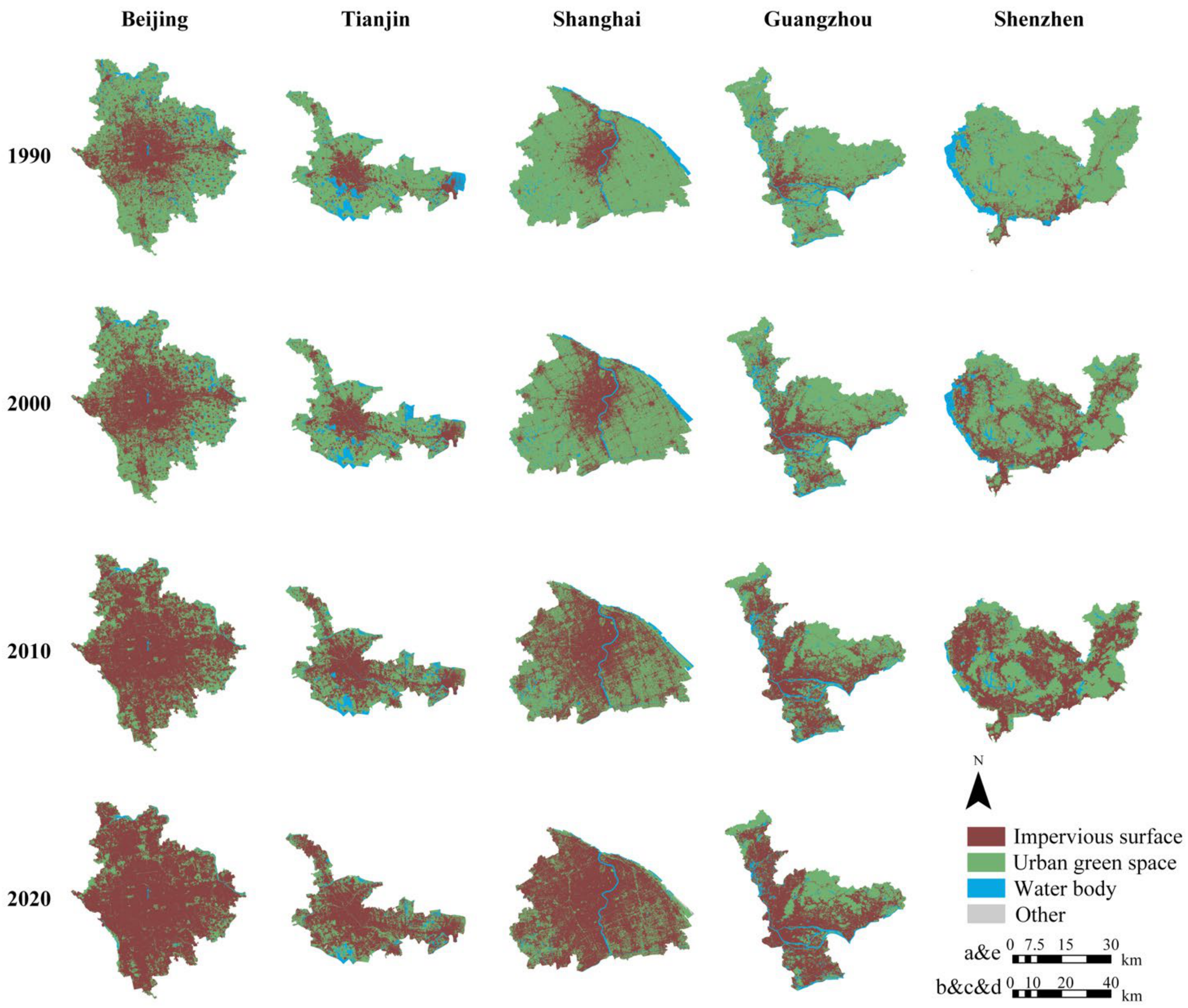
Based on the satellite images, land cover classification maps for the five megacities were obtained. The results illustrated that the landscape pattern of each megacity had undergone significant changes in the past four decades (Figure 2). Corresponding to previous studies [61], impervious surfaces of the five megacities were concentrated in local central areas in 1990; then, they expanded outward rapidly and constantly invaded the surrounding green space during rapid urbanization. Impervious surfaces showed a continuous increasing trend in all five megacities, in which Shanghai and Beijing presented the most obvious diffusion patterns. From 1990 to 2020, the proportion of expanded impervious surfaces in Beijing, Tianjin, Shanghai, Guangzhou, and Shenzhen reached 47.12%, 40.63%, 56.70%, 42.79%, and 45.17%, respectively. In contrast, urban green space was greatly reduced, with declines of 44.92%, 27.63%, 54.67%, 41.74%, and 38.01%, respectively. It was quite easy to determine that the majority of urban built-up areas expanded at the cost of occupying urban green space. Interestingly, this paper found that the urban expansion of the five megacities presented similar characteristics, which could be divided into three stages: low-speed expansion around the central area from 1990 to 2000, high-speed expansion in the suburban area from 2000 to 2010, and low-speed expansion in the suburban area from 2010 to 2020. However, the spatial patterns of urban expansion in the five megacities were not consistent. Beijing and Shanghai showed classic ring-pattern expansion, while the other three presented ribbon patterns expanding in different directions. Moreover, the degree of fragmentation for impervious surface distribution in Shenzhen was the highest, while the percentage of impervious surface was the lowest.

3.2. Comparison of Urban Thermal Environment

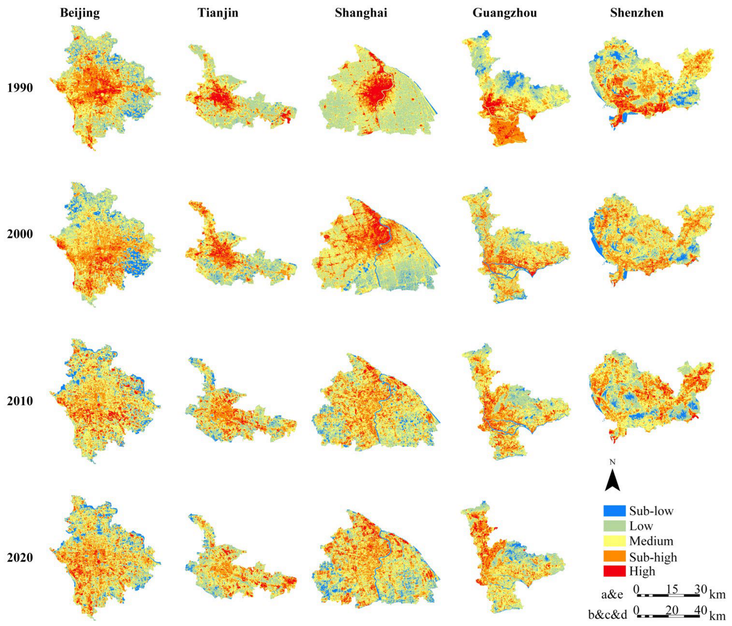
According to the classification results of the remotely sensed LST, the spatial distribution of the urban thermal landscape for five megacities from 1990 to 2020 is shown in Figure 3. The real value of mean LST and the raw Landsat thermal images can be found in Table A2. Figure A2 indicated the large-scale land-cover and thermal landscape maps of Beijing in 1990 and 2020, which illustrated an obvious expansion of impervious surface and more scattered sub-high temperature (S-H) areas (all large-scale images can be found in Supplementary Materials, Figures S1–S3). In 1990, the impervious surface as well as the S-H area mainly concentrated in the urban center, which occupied only 50% of the entire city area. While the impervious surface had continuously swallowed up the surrounding green space and became the absolute dominant land use type during the last three decades. Meanwhile, the S-H area dispersed with the increase of fragmentation degree of green patches, evenly spread over in the city. In general, the dynamic development trend of high (H) and sub-high temperature (S-H) areas in five megacities showed a similar trend. At the early stage of urban expansion in 1990, the H and S-H areas were mainly distributed in the urban central area. With the rapid expansion of impervious surfaces, the H and S-H areas gradually filled the whole study area, which spread continuously along the previous contour. In Figure 3, there is a clear phenomenon in which concentrated heat sources were transformed into numerous scattered but tiny thermal centers, which indicated that the spatial extents of UHI were no longer confined to megacity centers. However, the distribution patterns of scattered thermal patches in the five megacities were significantly different. In Beijing and Shanghai, which mainly expanded with the ring pattern, the H and S-H areas gradually spread around the city center. While the other three megacities mainly expanded in a ribbon pattern, the H and S-H areas generally expanded in one direction: Tianjin moved to the southwest, Guangzhou moved to the north, and Shenzhen moved to the northwest.
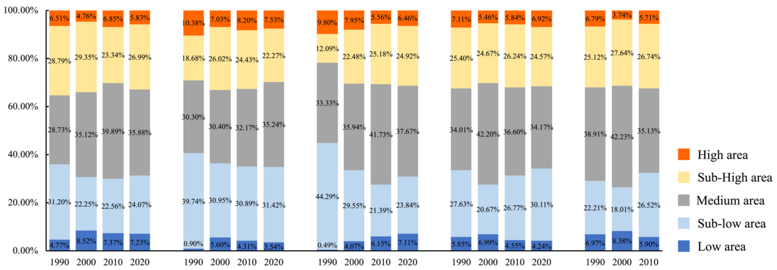
From the perspective of the proportion of various LST levels, the S-H area predominated over the urban thermal environment from 1990 to 2020 (Figure 4). In Guangzhou and Shenzhen, the proportion of medium-, sub-high-, and high-temperature areas decreased slightly from 1990 to 2020. In Beijing, Tianjin, and Shanghai, the area proportion increased from 64.0%, 59.4%, and 55.2% to 68.7%, 65.0%, and 69.1%, respectively. Although the proportion of high-temperature areas in most megacities showed a fluctuating downward trend, it should be noted that the decrease in the proportion of high-temperature areas was not due to improvement of urban thermal environment; rather, it was caused by the increase in the mean LST in the whole study area.

4. Discussion

4.1. Analysis of Landscape Composition and RLST within Buffer Zones

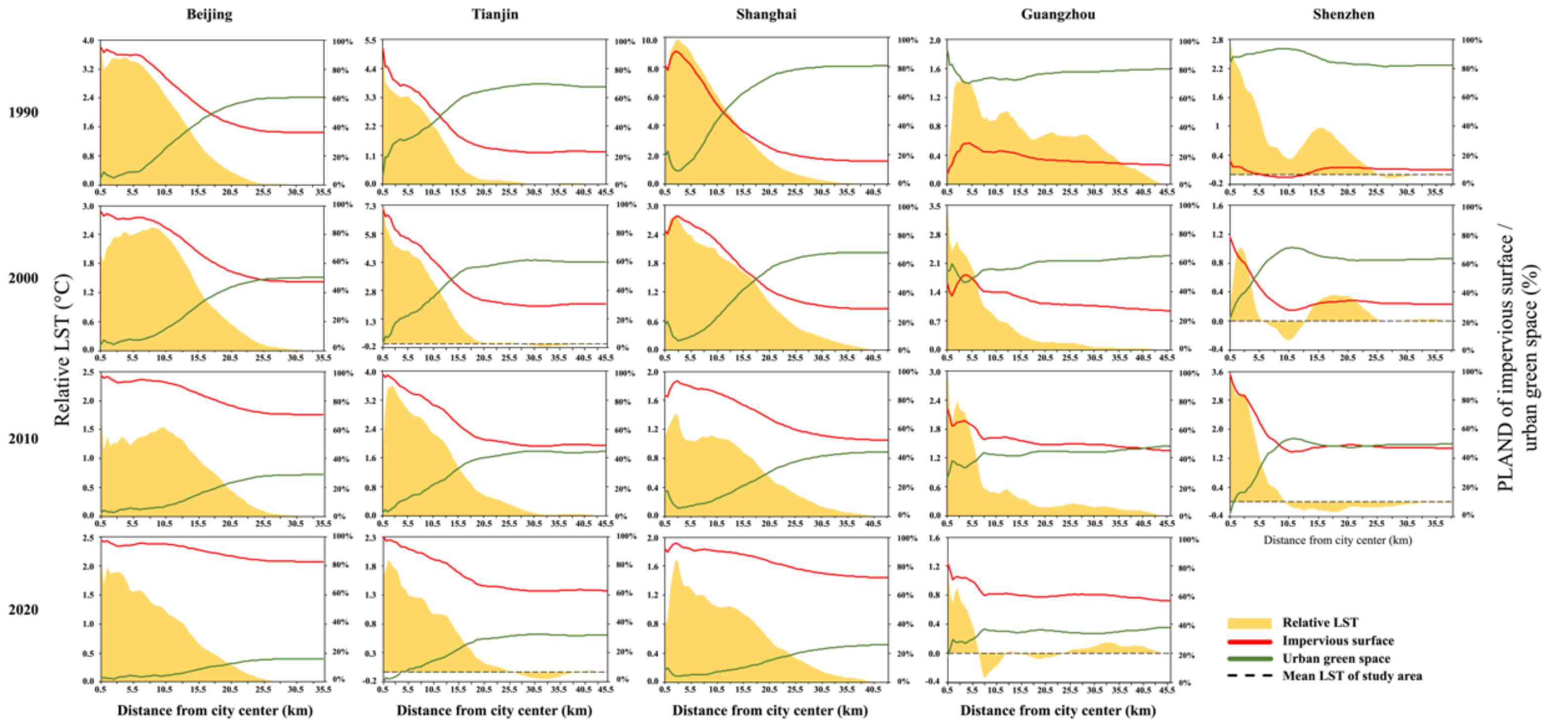
Concentric buffer zones were established to analyze the spatial patterns of both RLST and landscape composition from the city center to rural areas. The results indicated that there was a significant decreasing trend of RLST considering that the PLANDs of different landscape types both had a strong correlation with the urban thermal environment along the urban gradient (Figure 5 and Figure 6), which was also observed in other cities [39,62]. A rapid decrease in RLST corresponded to a sudden increase in urban green space in the buffer zones, which were approximately 10–15 km from the city center of each megacity. The highest decline in RLST of the four periods occurred in approximately 1990, and after that, the slope of the RLST curve gradually became smoother. This phenomenon explained why the high-temperature area showed a decreasing trend, which was observed in Section 3.2. The expansion of urban built-up areas intensified the UHI effect, and the significant high-temperature area was no longer limited to the city center. Notably, the largest increase in impervious surfaces for the five megacities started in 2000, and after that, the shape of the RLST curve transformed from “cliff” to “plains”.
Although there were numerous “peaks”, “plains”, and “valleys” for all RLST curves, only the curves of the three megacities with ribbon patterns in the last two decades, Tianjin, Guangzhou, and Shenzhen, contained the “basins”, which denoted that the mean LST within a certain buffer zone was lower than that of the whole study area (Figure 5). The “basins” indicated that the heterogeneous features of the urban thermal environment may be more sophisticated in a megacity with a non-ring-pattern because landscape composition and configuration were relatively homogeneous in ring-pattern cities compared with the ribbon-pattern or sector-pattern cities. It was interesting to note that there were two peaks of the RLST curve for Shenzhen both in 1990 and 2000, but then the second peak disappeared in 2010. Comparing this phenomenon with the urban expansion pattern in Shenzhen, we found that the multicentric expansion mode had been proposed by urban planning since the 1980s, and this mode lasted until the 2000s. Then, axial expansion dominated urban sprawl in Shenzhen after the 2000s, and the subcenter of Shenzhen was no longer obvious [63], resulting in the disappearance of the second peak in 2010.
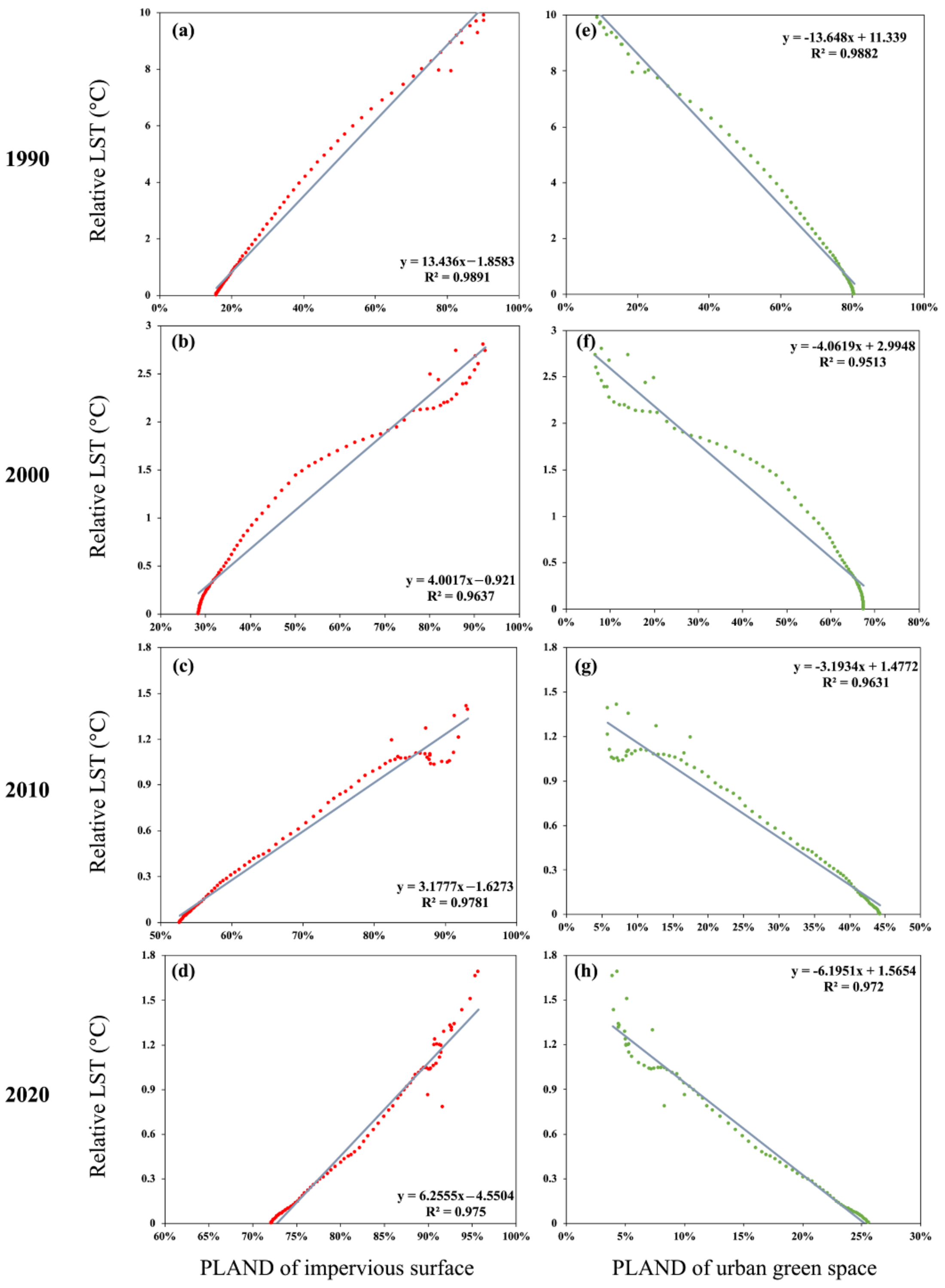
For further analysis, this paper selected Shanghai, one of the most developed megacities in China and even globally, to establish two linear regression models between two landscape types (impervious surface and urban green space) and RLST. The results confirmed that the RLST of the buffer zones was significantly correlated with the PLAND of both landscape types (Figure 6). The intercept value of curves (a)–(d) represents the RLST of a buffer zone with no impervious surface. The value decreased from −1.8583 to −4.5504, suggesting that the UHI effect would be more significant at a highly urbanized stage of the megacity due to the expansion of built-up areas. Interestingly, this paper found that the slope value of curves (a)–(d) decreased from 13.436 in 1990 to 6.256 in 2020. The decrease indicated that the PLAND, as the spatial metric of landscape composition, was less important at a highly urbanized stage, which has seldom been studied in previous research. To quantify the change in effects of landscape composition on the urban thermal environment, this paper then established a multivariable regression model and analyzed the variation in effects in the next two sections.

4.2. Effects of Landscape Patterns on LST

Landscape metrics can effectively quantify the structural composition and spatial configuration characteristics of impervious surfaces and urban green spaces. This paper selected 10 metrics for carrying out the bivariate analysis and establishing a ridge regression model between landscape pattern and LST. The Pearson correlation analysis indicated that most metrics were significantly related to LST at the 0.01 level, as shown in Table A4.
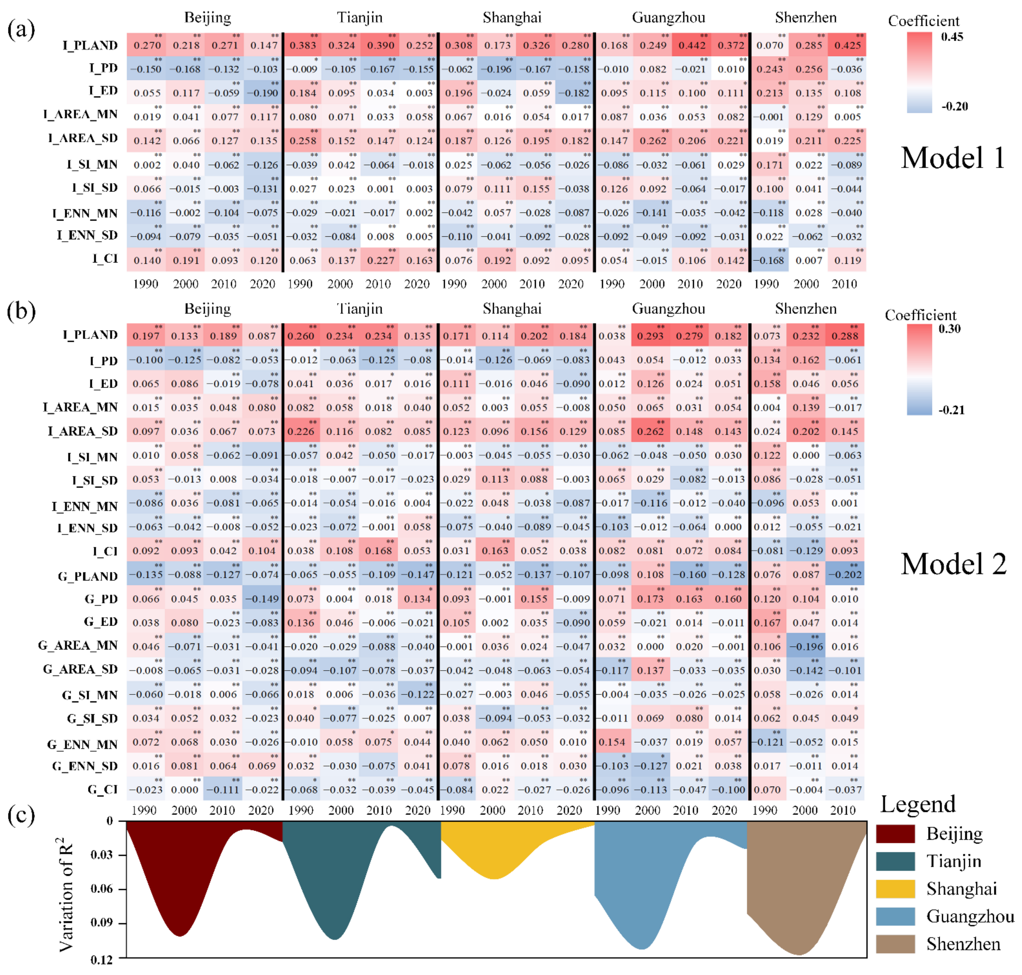
To compare the influence of impervious surfaces and urban green space on LST, this paper chose a hierarchical statistical model and established two layers (Figure 7). Model 1 was only for impervious surfaces, and Model 2 included urban green space metrics based on Model 1. Two layers both passed significance testing, which proved the effectiveness of the method. The interpretation results of the two models for LST are shown as below.
Model 1: The results showed that Model 1 could explain 37.69–87.01% of the variation in LST. Clearly, I_PLAND was the most important factor controlling the LST in Model 1. Among those configuration variables, I_PD and I_CI showed important but contrary effects in the urban thermal environment, with I_PD being negatively related to LST and I_CI being positively related to LST. Overall, LST increased with the growth of connectivity and edge density for impervious surface patches and decreased with the decline of nearest neighbor distances. Interestingly, the mean value and standard deviation of I_SI showed different correlations, suggesting that the effects of shape complexity on LST were complicated. The shape index should be maximized, but the variation in the shape index should be minimized when planning urban form.
Model 2: After adjusting for the metrics of impervious surfaces, the spatial metrics of the urban green space remained mostly significant. Among those spatial metrics, I_PLAND with a positive coefficient was still the most important. Meanwhile, G_PLAND was the most significant metric among the urban green space metrics and had a strong negative correlation with LST. In addition, G_AREA_SD and G_CI had a significant negative effect, indicating that LST decreased with increasing shape complexity and connectivity of green patches. This result might be because the increase in AREA_SD and CI of urban green space could increase shade and absorb heat from the surrounding environment through transpiration.
The increase in the R-square value brought by the increase in metrics of urban green space was relatively small. Approximately 1.84%~9.77% of the variation in LST was explained jointly by the urban green space metrics. The discrepancies in the R-square values between the two models confirmed that the importance of the impervious surface far exceeded that of urban green space, which was also consistent with the results of previous studies [39]. Despite the small variation in the R-square value, this paper surprisingly found that the variation experienced the largest increase in 2000 among all five megacities (Figure 7), and the year 2000 was exactly the initial point of the rapid urban expansion stage. This result indicated that the importance of the urban green space would reach its peak at the beginning of the period in which the urban areas started to expand rapidly.

4.3. Variations in the Effects of Landscape Patterns on the Urban Thermal Environment

In general, landscape composition was more important than landscape configuration in predicting the variation in LST, which was in line with previous studies [26,33,44,64]. However, this paper found that the standard regression coefficient of the landscape composition metric experienced an obvious decline from 1990 to 2020 (Figure 7). This tendency was similar to the relationships between RLST and PLAND of the two landscape types for Shanghai in Section 4.1. For example, the coefficient of I_PLAND in Model 2 decreased from the peak values of 0.27, 0.26, 0.20, and 0.29 to the minimum values of 0.09, 0.13, 0.18, and 0.18 for Beijing, Tianjin, Shanghai, and Guangzhou, respectively. In contrast, some landscape configuration metrics for both impervious surfaces and urban green spaces, such as PD, SI_MN, and CI, played more important roles in determining the urban thermal environment. The variation in the effects of landscape patterns on the urban thermal environment indicated that the effect of a single metric could be easily changed during rapid urbanization.
The year 2010 was a turning point, before which the speed of impervious surface growth was very high (Table 3), indicating that megacities had experienced intensified urban expansion from 1990 to 2010. During this period, the coefficients of PLAND in Model 1 basically remained unchanged or slightly fluctuated, presenting large values. After 2010, megacities entered the mature urbanization stage [65] and the speed of urban expansion flattened, in which the coefficients of the PLAND decreased significantly. Not only did the value of the coefficients vary with urban development, but the negative/positive correlations between some configuration metrics and LST also changed. ED, SI, and ENN transformed from negative to positive or from positive to negative. It can be concluded that the negative or positive correlation between one metric and LST was not constant but varied in different cities of different years (Table 4 and Table A3). This result may explain why some studies found that the cooling effects of green space were not significant, or even negative [66,67]. Previous studies noted that how to define the cooling effect may be related to the positive or negative cooling effect of green space [68,69,70]. This paper emphasized that the study area and data acquisition time may also affect the cooling effect, which may be caused by urban terrain, urban climate conditions or urbanization stages.
In addition to the processes of urbanization, urban patterns could bring variations in the effects. Compared with the three ribbon-pattern cities, the configuration metrics were more important, while the composition metric was less significant in ring-pattern megacities (Beijing and Shanghai). Further studies that investigated the relationships between urban forms and the effects are desirable. In addition, comparison studies concentrating on different climatic conditions are recommended.

4.4. Management Implications

Many studies have emphasized the importance of both landscape composition and configuration in mitigating UHI [39,44,71]. However, due to the absence of multicity and multiperiod comparison studies, the suggestion was not specific to different urbanization stages and was even contrary in how to improve landscape patterns. Thus, investigating variations in the effects was very instructive in improving the urban thermal environment by effective and targeted urban planning. For cities at a highly urbanized stage, such as those global metropolises, optimizing landscape configuration should have a high priority. On the one hand, transforming built-up areas into green space might be expensive and impractical. On the other hand, the composition of the landscape was less important at this stage than before. Simply changing the landscape composition, such as increasing the urban green space and restricting impervious surface expansion, was not an effective method to mitigate UHI. Considering the scarcity of land source in these megacities, constructing small-area green corridors or green belts, isolated green spaces can be connected to improve the area of a single patch, which can also increase connectivity and reduce the fragmentation of green patches. In addition, green roofs can be used to increase the fragmentation of impervious surface patches and thus reduce the area of a single impervious surface patch. For cities at the stage of rapid urban expansion, such as some medium-sized cities in China and some large cities in Southeast Asia, adequate urban green space should be reserved in advance during the process of urban expansion because the landscape composition at this stage has a crucial impact on the urban thermal environment. Compared with the ring-pattern expansion, the ribbon-pattern expansion can better meet this requirement. This pattern can retain enough green space around the impervious surface to improve urban thermal comfort and mitigate the UHI effect of urban built-up areas.
By the analysis of concentric buffer zones, this paper suggested that the large urban green park and green buffer zone may be constructed 10–15 km from the city center, such as the Beijing Olympic Forestry Park, because the cooling effect was most obvious at this distance. The urban green space within this range can effectively decrease the urban LST, improve the urban thermal environment, and act as an urban microclimate regulator.

5. Conclusions

Rapid urbanization has significantly changed landscape patterns and deteriorated the urban thermal environment, especially in megacities. Understanding the variation in the effects of landscape patterns on the urban thermal environment is critically important in mitigating UHI by reasonable urban planning for megacities. This paper selected the five largest megacities in China to quantitatively investigate the relationships between LST and the composition and configuration of urban landscapes and further analysed the variations in these effects from 1990 to 2020.
This comparative study indicated that landscape composition was more important than configuration in determining the urban thermal environment of all five megacities. However, the landscape configuration played increasingly important roles during rapid urbanization. On the one hand, the variation in the standard coefficients for landscape configuration indicated that not only did the value of coefficients fluctuate, but even the positive or negative characteristics of correlations might change during rapid urbanization. Spatial metrics that described shape complexity, patch density, and edge density showed contrary effects in determining the LST from 1990 to 2020. On the other hand, the variation in the R-square values between Model 1 and Model 2 indicated that for areas where rapid but unmatured urbanization is still in progress, such as some medium-size city of China or some cities of Southeast Asia, the ratio of urban green space to impervious surface should be highlighted in urban planning because the cooling effects of urban green space were the most significant in this period.
From the perspective of spatial arrangement, the analysis of concentric buffer zones depicted a typical urban thermal environmental profile, suggesting that the LST in the region approximately 10–15 km from the city center immediately declined from the peak values. This phenomenon indicated that urban green space in this region could significantly cool down the LST and improve the thermal environment in urban areas. The expansion patterns of impervious surfaces for the five megacities provided insight into mitigating UHI by transforming the ring-like form to the ribbon-like form. The ribbon pattern of impervious surfaces in Tianjin, Guangzhou, and Shenzhen can effectively decrease extra-high-temperature areas and balance the distribution of low-temperature areas. In addition, a single-center pattern of urban expansion may be negative in terms of mitigating UHIs compared with a multi-center or ribbon-form pattern.
Hence, for urban planners and natural resource managers, it is critically important to choose flexible and targeted strategies according to the local development level and urbanization stage. In the early stage of urbanization, the percentage of urban green space should be emphasized. For highly urbanized megacities, optimizing landscape configurations can improve the urban thermal environment efficiently at a relatively low cost, such as roof greening, vertical greening, and small green corridors. While this paper found variation in the effects on the urban thermal environment, it should be noted that this conclusion was based only on satellite images of megacities without considering climate conditions. Therefore, further research across cities of different sizes or under varied climate conditions, using multi-seasonal thermal data, and creating multi-resolution grids for analysis is recommended.

Supplementary Materials

The following are available online at https://www.mdpi.com/article/10.3390/rs13173415/s1, Figure S1: Urban green space of megacities, Figure S2: Larger-scale of land cover maps, Figure S3: Larger-scale of LST maps.

Author Contributions

Conceptualization, H.Y.; methodology, Y.L. and H.Y.; validation, X.L. and D.M.; formal analysis, H.Y.; investigation, H.Y.; resources, H.Y.; data curation, H.Y. and N.Z.; writing—original draft preparation, Y.L., H.Y., Z.L. and X.L.; writing—review and editing, H.Y.; supervision, H.Y. and J.Z.; project administration, Y.L.; funding acquisition, Y.L. All authors have read and agreed to the published version of the manuscript.

Funding

This research was funded by the National Natural Science Foundation of China, grant number 41771182, and the National Earth System Science Data Center “High spatial and temporal resolution data of long-term positioning monitoring of urban ecology and human activities in Beijing”.

Data Availability Statement

Landsat images used in this paper can be obtained from https://earthexplorer.usgs.gov/ (accessed on 1 July 2021).

Acknowledgments

We thank Hongming He for his valuable suggestion in article writing. We also thank the efforts of anonymous reviewers and the editor for their valuable comments and suggestions to improve the quality of the paper.

Conflicts of Interest

The authors declare no conflict of interest.

Appendix A

Figure A1. The digital elevation model of five megacities.
Remotesensing 13 03415 g0a1
Figure A2. Large-scale map of land cover and LST for Beijing in 1990 and 2020.
Remotesensing 13 03415 g0a2
Table A1. Meteorological data for the image acquisition dates of the five megacities.
MegacityImage Acquisition DateMaximum Air TemperatureMinimum Air TemperatureRelative Humidity
Beijing1992/09/07 GMT 02:15 Local time 10:1530.813.755
1999/08/02 GMT 02:46 Local time 10:4632.518.864
2010/08/08 GMT 02:43 Local time 10:4330.721.174
2019/08/17 GMT 02:53 Local time 10:5332.318.936
Tianjin1991/08/13 GMT 02:11 Local time 10:1128.921.374
1999/08/11 GMT 02:40 Local time 10:4031.822.666
2011/08/04 GMT 02:36 Local time 10:3631.022.067
2020/08/28 GMT 02:47 Local time 10:4730.520.076
Shanghai1989/08/11 GMT 01:51 Local time 09:5135.326.177
2000/08/01 GMT 02:15 Local time 10:1532.227.069
2007/07/28 GMT 02:18 Local time 10:1837.128.961
2020/08/16 GMT 02:24 Local time 10:2437.028.162
Guangzhou1989/07/06 GMT 02:19 Local time 10:1935.626.067
2000/09/14 GMT 02:42 Local time 10:4230.720.363
2008/07/26 GMT 02:38 Local time 10:3837.727.577
2019/09/27 GMT 02:52 Local time 10:5232.619.870
Shenzhen1989/07/06 GMT 02:19 Local time 10:1934.626.342
2000/09/14 GMT 02:42 Local time 10:4232.023.667
2008/07/26 GMT 02:38 Local time 10:3833.727.773
----
Table A2. The real value of mean LST derived from Landsat thermal images.
T/°CBeijingTianjinShanghaiGuangzhouShenzhen
199030.0530.7131.1430.9131.31
200030.9030.9431.2230.5930.58
201031.3430.7430.3231.5631.48
202030.6430.5931.4930.58-
Table A3. Pearson correlation coefficients between the relative land surface temperature (RLST) and spatial metrics.
Landscape PatternsSpatial MetricsBeijingTianjinShanghaiGuangzhouShenzhen
1990200020102020199020002010202019902000201020201990200020102020199020002010
CompositionI_PLAND0.941 **0.700 **0.814 **0.820 **0.905 **0.871 **0.882 **0.682 **0.964 **0.869 **0.874 **0.669 **0.838 **0.844 **0.767 **0.595 **0.846 **0.702 **0.471 **
G_PLAND−0.916 **−0.682 **−0.799 **−0.810 **−0.765 **−0.748 **−0.775 **−0.677 **−0.938 **−0.655 **−0.832 **−0.844 **−0.596 **−0.505 **−0.800 **−0.811 **−0.152−0.582 **−0.823 **
ConfigurationI_PD−0.789 **−0.651 **−0.744 **−0.706 **−0.193 *−0.492 **−0.668 **−0.617 **−0.468 **−0.625 **−0.813 **−0.787 **−0.021−0.133−0.346 **−0.373 **0.466 **0.073−0.370 **
I_ED0.123−0.081−0.627 **−0.819 **0.539 **0.307 **−0.215 *−0.328 **0.599 **0.054−0.158 **−0.735 **0.431 **0.396 **0.222 **0.153 *0.615 **0.559 **0.378 **
I_AREA_MN0.482 **0.400 **0.570 **0.638 **0.567 **0.586 **0.499 **0.429 **0.631 **0.325 **0.475 **0.580 **0.407 **0.336 **0.474 **0.515 **0.253 *0.475 **0.422 **
I_AREA_SD0.761 **0.551 **0.735 **0.768 **0.773 **0.744 **0.700 **0.577 **0.790 **0.567 **0.715 **0.789 **0.516 **0.560 **0.678 **0.713 **0.277 **0.580 **0.670 **
I_SHAPE_MN0.573 **0.428 **0.340 **0.1390.523 **0.654 **0.382 **0.370 **0.768 **0.367 **0.472 **0.361 **0.363 **0.354 **0.366 **0.352 **0.436 **0.337 **0.301 **
I_SHAPE_SD0.808 **0.563 **0.012−0.448 **0.667 **0.645 **0.278 **0.1080.832 **0.517 **0.621 **0.0130.503 **0.482 **0.333 **0.281 **0.431 **0.495 **0.482 **
I_ENN_MN−0.781 **−0.536 **−0.557 **−0.472 **−0.342 **−0.475 **−0.389 **−0.384 **−0.687 **−0.155 **−0.121 *−0.021−0.394 **−0.351 **−0.443 **−0.268 **−0.395 **−0.453 **−0.476 **
I_ENN_SD−0.773 **−0.552 **−0.580 **−0.544 **−0.377 **−0.453 **−0.388 **−0.484 **−0.715 **−0.142 *−0.282 **−0.157 **−0.377 **−0.375 **−0.436 **−0.439 **−0.338 **−0.427 **−0.432 **
I_COHESION0.822 **0.656 **0.672 **0.704 **0.541 **0.637 **0.700 **0.500 **0.725 **0.539 **0.642 **0.629 **0.411 **0.472 **0.459 **0.627 **0.259 **0.448 **0.625 **
G_PD0.840 **0.612 **0.068−0.450 **0.786 **0.707 **0.482 **0.215 *0.873 **0.553 **0.710 **0.0900.572 **0.605 **0.660 **0.599 **0.367 **0.608 **0.634 **
G_ ED0.053−0.104−0.630 **−0.824 **0.511 **0.240 **−0.307 **−0.402 **0.587 **0.041−0.179 **−0.741 **0.431 **0.311 **0.175 **0.0740.616 **0.546 **0.327 **
G_ AREA_MN−0.688 **−0.636 **−0.704 **−0.635 **−0.605 **−0.575 **−0.708 **−0.492 **−0.683 **−0.395 **−0.518 **−0.680 **−0.375 **−0.328 **−0.449 **−0.540 **−0.212 *−0.608 **−0.455 **
G_ AREA_SD−0.803 **−0.679 **−0.682 **−0.595 **−0.754 **−0.742 **−0.771 **−0.584 **−0.847 **−0.577 **−0.739 **−0.706 **−0.531 **−0.394 **−0.646 **−0.695 **−0.258 **−0.674 **−0.711 **
G_ SHAPE_MN−0.669 **−0.471 **−0.514 **−0.646 **−0.347 **−0.558 **−0.547 **−0.515 **−0.558 **−0.416 **−0.544 **−0.647 **−0.238 **−0.280 **−0.451 **−0.511 **0.112−0.216 *−0.272 **
G_ SHAPE_SD−0.659 **−0.518 **−0.639 **−0.610 **−0.176 *−0.461 **−0.594 **−0.549 **−0.344 **−0.577 **−0.755 **−0.764 **−0.092−0.115−0.297 **−0.402 **0.424 **0.068−0.210 *
G_ ENN_MN0.707 **0.489 **0.589 **0.648 **−0.159−0.163 *0.178 *0.413 **0.435 **0.434 **0.400 **0.468 **0.0940.1400.377 **0.416 **−0.323 **−0.0490.295 **
G_ ENN_SD0.702 **0.514 **0.588 **0.559 **0.517 **0.1390.0710.371 **0.759 **0.507 **0.397 **0.493 **0.173 *0.152 *0.391 **0.383 **−0.0660.243 **0.354 **
G_ COHESION−0.702 **−0.507 **−0.708 **−0.624 **−0.677 **−0.668 **−0.645 **−0.525 **−0.754 **−0.531 **−0.623 **−0.670 **−0.517 **−0.537 **−0.653 **−0.705 **−0.156−0.478 **−0.575 **
a “I_” denotes that the metric is calculated based on the landscape of impervious surface. “G_” denotes that the metric is calculated based on the landscape of urban green space. ** Coefficient is significant at 0.01 level (two-tailed). * Coefficient is significant at 0.05 level (two -tailed). Bold denotes the spatial metric is not significant.
Table A4. Variations of R2 between Models 1 and 2 in each megacity from approximately 1990 to approximately 2020.
R2BeijingTianjinShanghaiGuangzhouShenzhen
1990200020102020199020002010202019902000201020201990200020102020199020002010
Model 10.8701 0.5186 0.6485 0.7557 0.8113 0.7435 0.7703 0.4687 0.9311 0.4813 0.7907 0.7585 0.3767 0.5150 0.6974 0.7012 0.4434 0.5804 0.6942
Model 20.8760 0.6023 0.6581 0.7699 0.8279 0.8305 0.7747 0.5107 0.9449 0.5235 0.8051 0.7604 0.4310 0.6072 0.7121 0.7204 0.5136 0.6781 0.7042
Variation0.0059 0.0837 0.0096 0.0143 0.0166 0.0870 0.0044 0.0420 0.0138 0.0422 0.0144 0.0018 0.0543 0.0922 0.0146 0.0191 0.0702 0.0977 0.0099

References

  1. Kuang, W.; Chi, W.; Lu, D.; Dou, Y. A comparative analysis of megacity expansions in China and the U.S.: Patterns, rates and driving forces. Landsc. Urban Plan. 2014, 132, 121–135. [Google Scholar] [CrossRef]
  2. United Nations Department of Economic and Social Affairs (UNDESA). World Urbanization Prospects: The 2017 Revision; United Nations Publications: New York, NY, USA, 2018. [Google Scholar]
  3. The World Bank. Health Nutrition and Population Statistics by Wealth Quintile, World Bank Group. 2020. Available online: https://datacatalog.worldbank.org/dataset/health-nutrition-and-population-statistics-wealth-quintile (accessed on 2 July 2021).
  4. Tenedório, J.A.; Rebelo, C.; Estanqueiro, R.; Henriques, C.D.; Marques, L.; Gonçalves, J.A. New developments in geographical information technology for urban and spatial planning. In Technologies for Urban and Spatial Planning: Virtual Cities and Territories; IGI Global: Hershey, PA, USA, 2016; pp. 196–227. [Google Scholar] [CrossRef]
  5. Tenedório, J.A.; Estanqueiro, R.; Henriques, C.D. (Eds.) Methods and Applications of Geospatial Technology in Sustainable Urbanism; IGI Global: Hershey, PA, USA, 2016; pp. 34–56. [Google Scholar] [CrossRef]
  6. Liu, Y.T.; He, S.J.; Wu, F.L.; Webster, C. Urban villages under China’s rapid urbanization: Unregulated assets and transitional neighbourhoods. Habitat Int. 2010, 34, 135–144. [Google Scholar] [CrossRef]
  7. Gage, E.A.; Cooper, D.J. Relationships between landscape pattern metrics, vertical structure and surface urban Heat Island formation in a Colorado suburb. Urban Ecosyst. 2017, 20, 1229–1238. [Google Scholar] [CrossRef]
  8. Yin, C.H.; Yuan, M.; Lu, Y.P.; Huang, Y.P.; Liu, Y.F. Effects of urban form on the urban heat island effect based on spatial regression model. Sci. Total Environ. 2018, 634, 696–704. [Google Scholar] [CrossRef]
  9. Cui, Y.P.; Xu, X.L.; Dong, J.W.; Qin, Y.C. Influence of urbanization factors on surface urban heat island intensity: A comparison of countries at different developmental phases. Sustainability 2016, 8, 706. [Google Scholar] [CrossRef] [Green Version]
  10. Voogt, J.A.; Oke, T.R. Thermal remote sensing of urban climates. Remote Sens. Environ. 2003, 86, 370–384. [Google Scholar] [CrossRef]
  11. Luck, M.; Wu, J.G. A gradient analysis of urban landscape pattern: A case study from the Phoenix metropolitan region, Arizona, USA. Landsc. Ecol. 2002, 17, 327–339. [Google Scholar] [CrossRef]
  12. Santamouris, M.; Cartalis, C.; Synnefa, A.; Kolokotsa, D. On the impact of urban heat island and global warming on the power demand and electricity consumption of buildings—A review. Energy Build. 2015, 98, 119–124. [Google Scholar] [CrossRef]
  13. Yang, X.C.; Leung, L.R.; Zhao, N.Z.; Zhao, C.; Qian, Y.; Hu, K.J.; Liu, X.P.; Chen, B.D. Contribution of urbanization to the increase of extreme heat events in an urban agglomeration in east China. Geophys. Res. Lett. 2017, 44, 6940–6950. [Google Scholar] [CrossRef]
  14. Zang, J.L.; Guo, Q.Z.; Wu, X.X.; Sang, X.; Wu, H.H.; Qiao, Y. Integrated evaluation on multi-scale land surface temperature grading and bio-temperature suitability-a case study in Tianjin China. Int. J. Remote Sens. 2021, 42, 343–366. [Google Scholar] [CrossRef]
  15. Duneier, M. Ethnography, the ecological fallacy, and the 1995 Chicago heat wave. Am. Sociol. Rev. 2006, 71, 679–688. [Google Scholar] [CrossRef]
  16. Jenerette, G.D.; Harlan, S.L.; Buyantuev, A.; Stefanov, W.L.; Declet-Barreto, J.; Ruddell, B.L.; Myint, S.W.; Kaplan, S.; Li, X.X. Micro-scale urban surface temperatures are related to land-cover features and residential heat related health impacts in Phoenix, AZ USA. Landsc. Ecol. 2016, 31, 745–760. [Google Scholar] [CrossRef]
  17. Li, X.M.; Zhou, Y.Y.; Yu, S.; Jia, G.S.; Li, H.D.; Li, W.L. Urban heat island impacts on building energy consumption: A review of approaches and findings. Energy 2019, 174, 407–419. [Google Scholar] [CrossRef]
  18. Grimm, N.B.; Faeth, S.H.; Golubiewski, N.E.; Redman, C.L.; Wu, J.G.; Bai, X.M.; Briggs, J.M. Global change and the ecology of cities. Science 2008, 319, 756–760. [Google Scholar] [CrossRef] [PubMed] [Green Version]
  19. Gustafson, E.J. Quantifying landscape spatial pattern: What is the state of the art? Ecosystems 1998, 1, 143–156. [Google Scholar] [CrossRef]
  20. Turner, M.G. Landscape ecology: What is the state of the science? Annu. Rev. Ecol. Evol. Syst. 2005, 36, 319–344. [Google Scholar] [CrossRef]
  21. Arnfield, A.J. Two decades of urban climate research: A review of turbulence, exchanges of energy and water, and the urban heat island. Int. J. Clim. A J. R. Meteorol. Soc. 2003, 23, 1–26. [Google Scholar] [CrossRef]
  22. Alexander, C. Influence of the proportion, height and proximity of vegetation and buildings on urban land surface temperature. Int. J. Appl. Earth Obs. 2021, 95. [Google Scholar] [CrossRef]
  23. Deilami, K.; Kamruzzaman, M.; Liu, Y. Urban heat island effect: A systematic review of spatio-temporal factors, data, methods, and mitigation measures. Int. J. Appl. Earth Obs. 2018, 67, 30–42. [Google Scholar] [CrossRef]
  24. Guha, S.; Govil, H. An assessment on the relationship between land surface temperature and normalized difference vegetation index. Environ. Dev. Sustain. 2021, 23, 1944–1963. [Google Scholar] [CrossRef]
  25. Zhang, Y.; Sun, L.X. Spatial-temporal impacts of urban land use land cover on land surface temperature: Case studies of two Canadian urban areas. Int. J. Appl. Earth Obs. 2019, 75, 171–181. [Google Scholar] [CrossRef]
  26. Chen, A.L.; Yao, L.; Sun, R.H.; Chen, L.D. How many metrics are required to identify the effects of the landscape pattern on land surface temperature? Ecol. Indic. 2014, 45, 424–433. [Google Scholar] [CrossRef]
  27. Hart, M.; Sailor, D. Quantifying the influence of land-use and surface characteristics on spatial variability in the urban heat island. Appl. Clim. 2009, 95, 397–406. [Google Scholar] [CrossRef]
  28. Zhao, X.F.; Liu, J.H.; Liu, L.L. Cool island effects of urban green open spaces in the process of urbanization: A multi-temporal study of Xiamen Island. Int. Workshop Earth Obs. Remote Sens. Appl. IEEE 2016. [Google Scholar] [CrossRef]
  29. Zhao, Z.Q.; He, B.J.; Li, L.G.; Wang, H.B.; Darko, A. Profile and concentric zonal analysis of relationships between land use/land cover and land surface temperature: Case study of Shenyang, China. Energy Build. 2017, 155, 282–295. [Google Scholar] [CrossRef]
  30. Bokaie, M.; Zarkesh, M.K.; Arasteh, P.D.; Hosseini, A. Assessment of urban heat island based on the relationship between land surface temperature and land use/land cover in Tehran. Sustain. Cities Soc. 2016, 23, 94–104. [Google Scholar] [CrossRef]
  31. Pal, S.; Ziaul, S. Detection of land use and land cover change and land surface temperature in English Bazar urban centre. Egypt. J. Remote Sens. 2017, 20, 125–145. [Google Scholar] [CrossRef] [Green Version]
  32. Zhou, W.Q.; Qian, Y.G.; Li, X.M.; Li, W.F.; Han, L.J. Relationships between land cover and the surface urban heat island: Seasonal variability and effects of spatial and thematic resolution of land cover data on predicting land surface temperatures. Landsc. Ecol. 2014, 29, 153–167. [Google Scholar] [CrossRef]
  33. Connors, J.P.; Galletti, C.S.; Chow, W.T.L. Landscape configuration and urban heat island effects: Assessing the relationship between landscape characteristics and land surface temperature in Phoenix, Arizona. Landsc. Ecol. 2013, 28, 271–283. [Google Scholar] [CrossRef]
  34. Li, W.F.; Cao, Q.W.; Lang, K.; Wu, J.S. Linking potential heat source and sink to urban heat island: Heterogeneous effects of landscape pattern on land surface temperature. Sci. Total Environ. 2017, 586, 457–465. [Google Scholar] [CrossRef]
  35. Masoudi, M.; Tan, P.Y. Multi-year comparison of the effects of spatial pattern of urban green spaces on urban land surface temperature. Landsc. Urban Plan. 2019, 184, 44–58. [Google Scholar] [CrossRef]
  36. Hung, T.; Uchihama, D.; Ochi, S.; Yasuoka, Y. Assessment with satellite data of the urban heat island effects in Asian mega cities. Int. J. Appl. Earth Obs. 2006, 8, 34–48. [Google Scholar] [CrossRef]
  37. Peng, S.S.; Piao, S.L.; Ciais, P.; Friedlingstein, P.; Ottle, C.; Breon, F.M.; Nan, H.J.; Zhou, L.M.; Myneni, R.B. Response to comment on “Surface urban heat island across 419 global big cities”. Environ. Sci. Technol. 2012, 46, 6889–6890. [Google Scholar] [CrossRef]
  38. Yao, R.; Wang, L.; Huang, X.; Liu, Y.; Niu, Z.; Wang, S.; Wang, L. Long-term trends of surface and canopy layer urban heat island intensity in 272 cities in the mainland of China. Sci. Total Environ. 2021, 772, 145607. [Google Scholar] [CrossRef]
  39. Estoque, R.C.; Murayama, Y.; Myint, S.W. Effects of landscape composition and pattern on land surface temperature: An urban heat island study in the megacities of Southeast Asia. Sci. Total Environ. 2017, 577, 349–359. [Google Scholar] [CrossRef]
  40. Morabito, M.; Crisci, A.; Guerri, G.; Messeri, A.; Congedo, L.; Munafo, M. Surface urban heat islands in Italian metropolitan cities: Tree cover and impervious surface influences. Sci. Total Environ. 2021, 751, 142334. [Google Scholar] [CrossRef] [PubMed]
  41. Tran, D.X.; Pla, F.; Latorre-Carmona, P.; Myint, S.W.; Gaetano, M.; Kieu, H.V. Characterizing the relationship between land use land cover change and land surface temperature. ISPRS. J. Photogramm. 2017, 124, 119–132. [Google Scholar] [CrossRef] [Green Version]
  42. Guo, L.J.; Liu, R.M.; Men, C.; Wang, Q.R.; Miao, Y.X.; Zhang, Y. Quantifying and simulating landscape composition and pattern impacts on land surface temperature: A decadal study of the rapidly urbanizing city of Beijing, China. Sci. Total Environ. 2019, 654, 430–440. [Google Scholar] [CrossRef] [PubMed]
  43. Peng, J.; Xie, P.; Liu, Y.X.; Ma, J. Urban thermal environment dynamics and associated landscape pattern factors: A case study in the Beijing metropolitan region. Remote Sens. Environ. 2016, 173, 145–155. [Google Scholar] [CrossRef]
  44. Zhou, W.Q.; Huang, G.L.; Cadenasso, M.L. Does spatial configuration matter? Understanding the effects of land cover pattern on land surface temperature in urban landscapes. Landsc. Urban Plan. 2011, 102, 54–63. [Google Scholar] [CrossRef]
  45. Li, Y.; Ye, H.; Gao, X.; Sun, D.; Li, Z.; Zhang, N.; Leng, X.; Meng, D.; Zheng, J. Spatiotemporal patterns of urbanization in the three most developed urban agglomerations in china based on continuous nighttime light data (2000–2018). Remote Sens. 2021, 13, 2245. [Google Scholar] [CrossRef]
  46. Meng, Q.Y.; Zhang, L.L.; Sun, Z.H.; Meng, F.; Wang, L.; Sun, Y.X. Characterizing spatial and temporal trends of surface urban heat island effect in an urban main built-up area: A 12-year case study in Beijing, China. Remote Sens. Environ. 2018, 204, 826–837. [Google Scholar] [CrossRef]
  47. Peng, J.; Jia, J.L.; Liu, Y.X.; Li, H.L.; Wu, J.S. Seasonal contrast of the dominant factors for spatial distribution of land surface temperature in urban areas. Remote Sens. Environ. 2018, 215, 255–267. [Google Scholar] [CrossRef]
  48. Qiao, Z.; Liu, L.; Qin, Y.W.; Xu, X.L.; Wang, B.W.; Liu, Z.J. The Impact of urban renewal on land surface temperature changes: A case study in the main city of Guangzhou, China. Remote Sens. 2020, 12, 794. [Google Scholar] [CrossRef] [Green Version]
  49. Yue, W.Z.; Liu, X.; Zhou, Y.Y.; Liu, Y. Impacts of urban configuration on urban heat island: An empirical study in China mega-cities. Sci. Total Environ. 2019, 671, 1036–1046. [Google Scholar] [CrossRef]
  50. Zhou, D.C.; Bonafoni, S.; Zhang, L.X.; Wang, R.H. Remote sensing of the urban heat island effect in a highly populated urban agglomeration area in East China. Sci. Total Environ. 2018, 628, 415–429. [Google Scholar] [CrossRef]
  51. Wang, M.; Zhang, Z.; Hu, T.; Liu, X. A practical single-channel algorithm for land surface temperature retrieval: Application to landsat series data. J. Geophys. Res. Atmos. 2019, 124, 299–316. [Google Scholar] [CrossRef]
  52. Wang, M.; Zhang, Z.; Hu, T.; Wang, G.; He, G.; Zhang, Z.; Li, H.; Wu, Z.; Liu, X. An efficient framework for producing landsat-based land surface temperature data using Google Earth Engine. IEEE J. Sel. Top. Appl. Earth Obs. Remote Sens. 2020, 13, 4689–4701. [Google Scholar] [CrossRef]
  53. Weng, Q. Thermal infrared remote sensing for urban climate and environmental studies: Methods, applications, and trends. ISPRS J. Photogramm. Remote Sens. 2009, 64, 335–344. [Google Scholar] [CrossRef]
  54. Ren, H.; Du, C.; Liu, R.; Qin, Q.; Yan, G.; Li, Z.-L.; Meng, J. Atmospheric water vapor retrieval from Landsat 8 thermal infrared images. J. Geophys. Res. Atmos. 2015, 120, 1723–1738. [Google Scholar] [CrossRef]
  55. Wang, M.; He, G.; Zhang, Z.; Wang, G.; Long, T. NDVI-based split-window algorithm for precipitable water vapour retrieval from Landsat-8 TIRS data over land area. Remote Sens. Lett. 2015, 6, 904–913. [Google Scholar] [CrossRef]
  56. Sobrino, J.A.; Jimenez-Munoz, J.C.; Soria, G.; Romaguera, M.; Guanter, L.; Moreno, J.; Plaza, A.; Martincz, P. Land surface emissivity retrieval from different VNIR and TIR sensors. IEEE Trans. Geosci. Remote Sens. 2008, 46, 316–327. [Google Scholar] [CrossRef]
  57. Huete, A.; Didan, K.; Miura, T.; Rodriguez, E.P.; Gao, X.; Ferreira, L.G. Overview of the radiometric and biophysical performance of the MODIS vegetation indices. Remote Sens. Environ. 2002, 83, 195–213. [Google Scholar] [CrossRef]
  58. Sobrino, J.A.; Raissouni, N. Toward remote sensing methods for land cover dynamic monitoring: Application to Morocco. Int. J. Remote Sens. 2000, 21, 353–366. [Google Scholar] [CrossRef]
  59. Seto, K.C.; Fragkias, M. Quantifying spatiotemporal patterns of urban land-use change in four cities of china with time series landscape metrics. Landsc. Ecol. 2005, 20, 871–888. [Google Scholar] [CrossRef]
  60. Tian, G.; Jiang, J.; Yang, Z.; Zhang, Y. The urban growth, size distribution and spatio-temporal dynamic pattern of the Yangtze River Delta megalopolitan region, China. Ecol. Model. 2011, 222, 865–878. [Google Scholar] [CrossRef]
  61. Kuang, W. 70 years of urban expansion across China: Trajectory, pattern, and national policies. Sci. Bull. 2020, 65, 1970–1974. [Google Scholar] [CrossRef]
  62. Xiao, R.; Ouyang, Z.; Zheng, H.; Li, W.; Schienke, E.W.; Wang, X. Spatial pattern of impervious surfaces and their impacts on land surface temperature in Beijing, China. J. Environ. Sci. 2007, 19, 250–256. [Google Scholar] [CrossRef]
  63. Fei, W.; Zhao, S. Urban land expansion in China’s six megacities from 1978 to 2015. Sci. Total Environ. 2019, 664, 60–71. [Google Scholar] [CrossRef]
  64. Li, X.; Zhou, W.; Ouyang, Z.; Xu, W.; Zheng, H. Spatial pattern of greenspace affects land surface temperature: Evidence from the heavily urbanized Beijing metropolitan area, China. Landsc. Ecol. 2012, 27, 887–898. [Google Scholar] [CrossRef]
  65. Li, Y.; Ye, H.; Sun, X.; Zheng, J.; Meng, D. Coupling analysis of the thermal landscape and environmental carrying capacity of urban expansion in Beijing (China) over the past 35 years. Sustainability 2021, 13, 584. [Google Scholar] [CrossRef]
  66. Santamouris, M.; Ban-Weiss, G.; Osmond, P.; Paolini, R.; Synnefa, A.; Cartalis, C.; Muscio, A.; Zinzi, M.; Morakinyo, T.E.; Ng, E.; et al. Progress in urban greenery mitigation science—Assessment methodologies advanced technologies and impact on cities. J. Civ. Eng. Manag. 2018, 24, 638–671. [Google Scholar] [CrossRef] [Green Version]
  67. Yu, Z.; Yao, Y.; Yang, G.; Wang, X.; Vejre, H. Spatiotemporal patterns and characteristics of remotely sensed region heat islands during the rapid urbanization (1995–2015) of Southern China. Sci. Total Environ. 2019, 674, 242–254. [Google Scholar] [CrossRef]
  68. Fan, H.; Yu, Z.; Yang, G.; Liu, T.Y.; Liu, T.Y.; Hung, C.H.; Vejre, H. How to cool hot-humid (Asian) cities with urban trees? An optimal landscape size perspective. Agric. For. Meteorol. 2019, 265, 338–348. [Google Scholar] [CrossRef]
  69. Lin, W.; Yu, T.; Chang, X.; Wu, W.; Zhang, Y. Calculating cooling extents of green parks using remote sensing: Method and test. Landsc. Urban Plan. 2015, 134, 66–75. [Google Scholar] [CrossRef]
  70. Yu, Z.; Guo, X.; Jorgensen, G.; Vejre, H. How can urban green spaces be planned for climate adaptation in subtropical cities? Ecol. Indic. 2017, 82, 152–162. [Google Scholar] [CrossRef]
  71. Maimaitiyiming, M.; Ghulam, A.; Tiyip, T.; Pla, F.; Latorre-Carmona, P.; Halik, U.; Sawut, M.; Caetano, M. Effects of green space spatial pattern on land surface temperature: Implications for sustainable urban planning and climate change adaptation. ISPRS J. Photogramm. 2014, 89, 59–66. [Google Scholar] [CrossRef] [Green Version]
  72. Song, Y.; Song, X.; Shao, G. Effects of green space patterns on urban thermal environment at multiple spatial-temporal scales. Sustainability 2020, 12, 6850. [Google Scholar] [CrossRef]
  73. Chen, A.L.; Sun, R.H.; Chen, L.D. Applicability of traditional landscape metrics in evaluating urban heat island effect. J. Appl. Ecol. 2012, 23, 2077–2086. (in Chinese). [Google Scholar]
  74. Zhou, W.; Cao, F. Effects of changing spatial extent on the relationship between urban forest patterns and land surface temperature. Ecol. Indic. 2020, 109. [Google Scholar] [CrossRef]
  75. Asgarian, A.; Amiri, B.J.; Sakieh, Y. Assessing the effect of green cover spatial patterns on urban land surface temperature using landscape metrics approach. Urban Ecosyst. 2015, 18, 209–222. [Google Scholar] [CrossRef]
  76. Cao, X.; Onishi, A.; Chen, J.; Imura, H. Quantifying the cool island intensity of urban parks using ASTER and IKONOS data. Landsc. Urban Plan. 2010, 96, 224–231. [Google Scholar] [CrossRef]
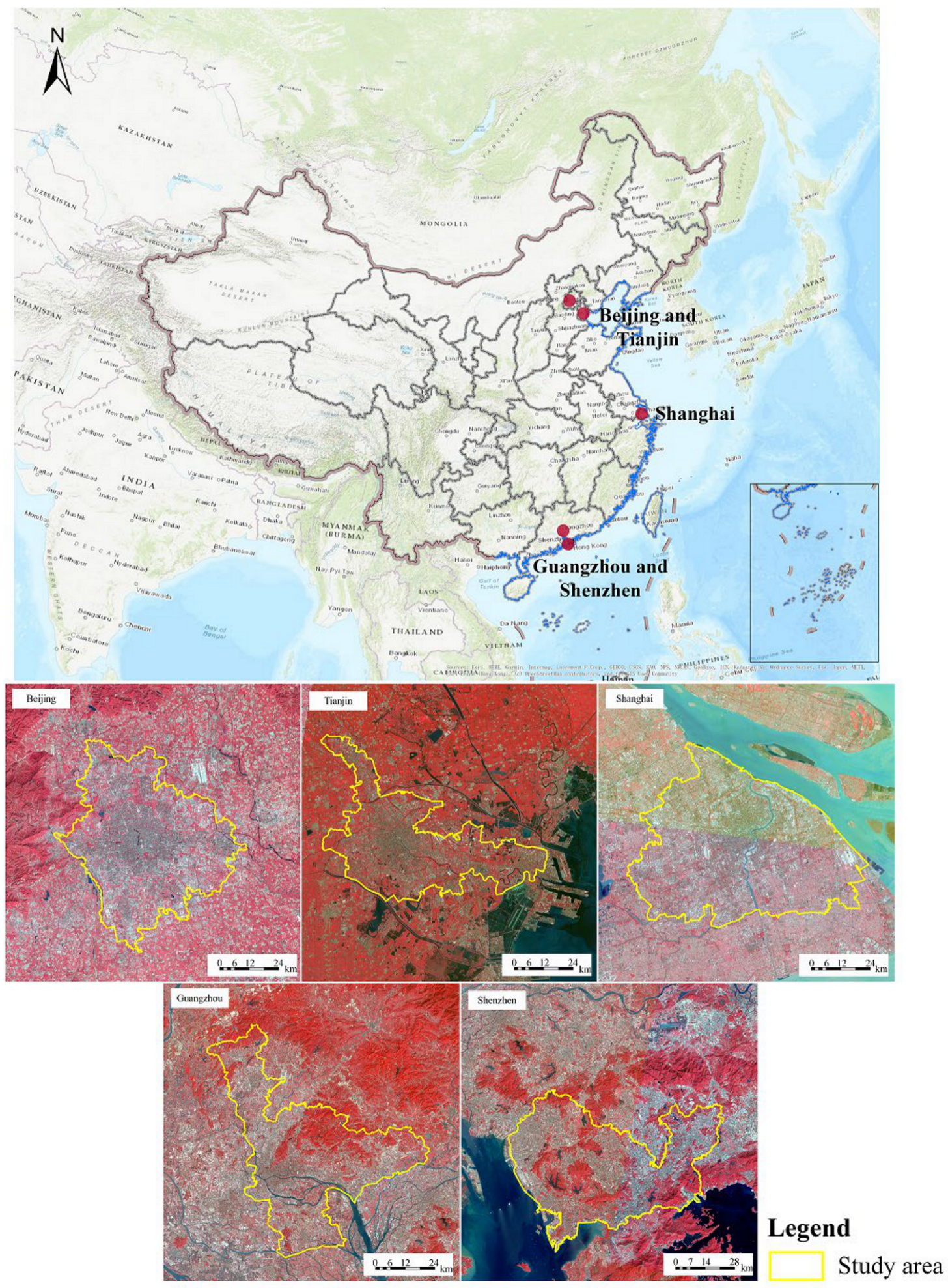
Figure 1. The locations of five megacities: Beijing, Tianjin, Shanghai, Guangzhou, and Shenzhen.
Remotesensing 13 03415 g001
Figure 2. Land cover classification maps for five megacities from approximately 1990 to approximately 2020. From the left panel to the right panel: Beijing, Tianjin, Shanghai, Guangzhou, and Shenzhen.
Remotesensing 13 03415 g002
Figure 3. Spatial distribution of urban thermal landscape classified by remotely sensed LST for five megacities from approximately 1990 to approximately 2020. From the left panel to the right panel: Beijing, Tianjin, Shanghai, Guangzhou, and Shenzhen.
Remotesensing 13 03415 g003
Figure 4. The variation in the percentage of the five LST levels for each megacity from 1990 to 2020.
Remotesensing 13 03415 g004
Figure 5. A comparison of the variation in the RLST and PLAND of impervious surfaces and urban green spaces in concentric buffer zones of five megacities.
Remotesensing 13 03415 g005
Figure 6. Relationships between the PLAND of two landscape types and RLST in Shanghai from 1990 to 2020. (ad): PLAND of impervious surface vs. RLST from 1990 to 2020, (eh): PLAND of urban green space vs. RLST from 1990 to 2020.
Remotesensing 13 03415 g006
Figure 7. (a,b) Correlation coefficients of hierarchical ridge regression models. (c) The variation in R-square between the two models (Model 2 minus Model 1). ** Coefficient is significant at the 0.01 level (two-tailed). * Coefficient is significant at 0.05 level (two-tailed).
Remotesensing 13 03415 g007
Table 1. A summary of satellite images used in research and nature-social characteristics of study areas in each period.
MegacityImage Acquisition DateDatasetsPath-RowPopulation (Million)GDP (Billion $)
Beijing1992/09/07 GMT 02:15 Local time 10:15Landsat 5 TM123-3210.8610.47
1999/08/02 GMT 02:46 Local time 10:46Landsat 7 ETM123-3213.6438.80
2010/08/08 GMT 02:43 Local time 10:43Landsat 5 TM123-3219.62211.50
2019/08/17 GMT 02:53 Local time 10:53Landsat 8 TIRSI123-3221.54512.82
Tianjin1991/08/13 GMT 02:11 Local time 10:11Landsat 5 TM122-338.846.50
1999/08/11 GMT 02:40 Local time 10:40Landsat 7 ETM122-3310.0120.56
2011/08/04 GMT 02:36 Local time 10:36Landsat 5 TM122-3312.99135.10
2020/08/28 GMT 02:47 Local time 10:47Landsat 8 TIRSI122-3315.62204.49
Shanghai1989/08/11 GMT 01:51 Local time 09:51Landsat 5 TM118-3813.3416.34
2000/08/01 GMT 02:15 Local time 10:15Landsat 7 ETM118-3816.0958.12
2007/07/28 GMT 02:18 Local time 10:18Landsat 5 TM118-3823.03255.37
2020/08/16 GMT 02:24 Local time 10:24Landsat 8 TIRSI118-3824.28553.18
Guangzhou1989/07/06 GMT 02:19 Local time 10:19Landsat 5 TM122-445.926.68
2000/09/14 GMT 02:42 Local time 10:42Landsat 7 ETM122-449.9530.26
2008/07/26 GMT 02:38 Local time 10:38Landsat 5 TM122-4412.71155.84
2019/09/27 GMT 02:52 Local time 10:52Landsat 8 TIRSI122-4428.74342.57
Shenzhen1989/07/06 GMT 02:19 Local time 10:19Landsat 5 TM122-441.683.59
2000/09/14 GMT 02:42 Local time 10:42Landsat 7 ETM122-447.0126.80
2008/07/26 GMT 02:38 Local time 10:38Landsat 5 TM122-4410.37147.47
---12.52392.97
Table 2. Spatial metrics used in this study to measure landscape patterns.
Spatial MetricsAbbreviationDescription
Composition
Percent of landscapePLANDThe percentage of each landscape type
Configuration
Patch densityPDThe patch number of each landscape per unit area
Edge densityEDThe total length of each landscape per unit area
Mean patch areaAREA_MNReflecting the patch area or size of each landscape type
Standard deviation of patch areaAREA_SDA measure of the variability of patch area or size
Mean shape indexSI_MNA straightforward measure of shape complexity
Standard deviation of shape indexSI_SDA measure of the variability of shape complexity
Mean Euclidian nearest neighbor distanceENN_MNThe average distance of one landscape patch to its nearest neighbor patch of the same landscape
Standard deviation of Euclidian nearest neighbor distanceENN_SDA measure of the variability of nearest neighbor distance
Patch cohesionCIReflecting the dispersion and interspersion of the landscape
Table 3. The proportion and annual growth rate of impervious surfaces and urban green spaces from 1990 to 2020 in five megacities.
BeijingTianjinShanghaiGuangzhouShenzhen
Proportion of urban green space
199060.44%60.26%80.43%79.62%82.34%
200050.33%67.21%67.59%65.04%63.73%
201028.85%44.45%44.49%48.12%50.97%
202015.52%32.63%25.76%37.88%44.33%
Annual growth rate of urban green space
1990–2000−1.81%1.10%−1.72%−2.00%−2.53%
2000–2010−5.41%−4.05%−4.10%−2.97%−2.21%
2010–2020−6.01%−3.04%−5.32%−2.36%−1.39%
1990–2020−4.43%−2.02%−3.72%−2.45%−2.04%
Proportion of impervious surface
199036.00%22.43%15.74%13.36%10.04%
200047.19%30.47%28.47%27.24%31.88%
201070.20%48.68%52.87%45.25%48.01%
202083.12%63.06%72.44%56.15%55.21%
Annual growth rate of impervious surface
1990–20002.74%3.11%6.11%5.38%12.25%
2000–20104.05%4.80%6.39%7.21%4.18%
2010–20201.70%2.62%3.20%2.18%1.41%
1990–20202.83%3.51%5.22%4.90%5.85%
Table 4. Characteristics of the correlation between spatial metrics of two landscape types and LST in different years of different cities.
MetricCorrelation between Spatial Metrics and LSTStudy AreaAcquisition Year of DataReference
Impervious SurfaceUrban Green Space
Edge density (ED)PNBangkok, Jakarta, Manila, Southeast Asia2014[39]
NNBaltimore, USA1999[44]
-NAksu, China2011[71]
PPHangzhou, China2016[72]
-PBeijing, China2002[73]
Patch density (PD)-NAksu, China2011[71]
PNBangkok, Jakarta, Manila, Southeast Asia2014[39]
-PBeijing, China2002[73]
-PShanghai, China2017[74]
Shape index (SI)-NBaltimore, USA1999[44]
-NIsfahan, Iran2002[75]
-NNagoya, Japan2004[76]
-PHangzhou, China2016[72]
-PShanghai, China2016[74]
-PBeijing, China2002[73]
Note: “P” denotes a positive correlation, “N” denotes a negative correlation, and “-” denotes that the metric was not mentioned in the study.
Publisher’s Note: MDPI stays neutral with regard to jurisdictional claims in published maps and institutional affiliations.