Spatial Variations in Terrestrial Water Storage with Variable Forces across the Yellow River Basin

Abstract

Terrestrial water storage (TWS) variations are a result of the interconnected impact of various variables including climate, hydrology, ecology, and anthropogenic activities. Previous studies have indicated that climate factors (e.g., precipitation and potential evapotranspiration), vegetation restoration, and water withdrawals (irrigational and industrial water use) are the major determinants of TWS depletion across the Yellow River Basin (YRB). However, few studies have provided explicit information about the main forcing variables that determine spatiotemporal variations in TWS and the synergies among these factors. This study explored the explicit understanding of hydro-climatic and socio-ecological determinants and the key interacting processes that affected the TWS variations across the Yellow River Basin in northern China. The multivariate adaptive regression splines model was employed to establish the relationship function of the long-term trends for the dependent (TWS) and independent (explanatory) variables consisting of normalized difference vegetation index (NDVI), hydro-climate, and human water withdrawal. The long-term trends estimated from the MARS model reproduced the ones calculated by Gravity Recovery and Climate Experiment gravity satellites, with a determination coefficient (R²) of 0.83 and a mean absolute error (MAE) of 1.2 mm. The results showed that precipitation, minimum temperature, runoff, base flow, water withdrawal for electricity, and NDVI were the main drivers of the spatiotemporal variations in the TWS, of which minimum temperature and runoff played a considerable role in TWS variations through the interplay with other variables. The critical values of the trend for interactive variables, which could alter the acting direction of the synergy on the TWS, were also estimated. In view of the connotation of interactive variables, we suggested that spatiotemporal variations in TWS resulted from the coupling of the hydrological energy system, hydrological ecosystem, and hydrological system in the YRB, of which the hydrological system plays the most significant role, followed by the hydrological ecosystem.

1. Introduction

Terrestrial water storage (TWS) contains all types of water stored on land, including soil water, groundwater, lakes, rivers, and glaciers [1,2,3]. It plays an important role in the Earth’s climate system by exerting control over water, energy, and biogeochemical fluxes [4]. TWS change under natural conditions is the residual (precipitation, evapotranspiration, and discharge) of hydrological cycle fluxes in a certain period, which is regarded as a crucial hydrological indicator [5]. Compared with a single hydrological element, TWS is more suitable for tracing the change in water resources on land. Therefore, the monitoring of spatiotemporal variations in TWS and a comprehensive and clear understanding of driving mechanisms are beneficial for water resource management and sustainable water utilization.

The general means of observing water storage changes are field measurement, model simulation, and remote sensing inversion. Remote sensing inversion is superior to other methods on regional and global scales, considering its free and convenient access. The Gravity Recovery and Climate Experiment (GRACE) gravity satellite mission, launched in 2002 and ended in 2017, consisted of two satellites in a tandem orbit about 200 km apart and can monitor the time-variable gravity field anomaly caused by the change in earth surface mass. Removing the effect of oceanic and atmospheric circulations from earth mass change estimated by GRACE, the TWS anomaly (TWSA), which is relative to the average of some time periods, can be obtained [6,7]. Many studies have suggested that GRACE is an effective tool for monitoring TWS variations at global and regional scales [8,9,10,11,12]. TWS variations derived from GRACE contain the response to the disturbance of both climate and human activities [13,14,15,16], thus providing an opportunity to investigate the influence of climate and human activities and their interactions on TWS variations.

The Yellow River Basin (YRB) is mainly located in arid and semi-arid climate regions, where water restricts economic development and threatens ecological environment security [17,18]. Additionally, climate warming and increased water use have exacerbated the contradiction between water supply and demand in the YRB during recent decades [19]. The middle and upper reaches of the YRB, which covers most of the Loess Plateau, witnessed a great change in land cover and land use [20,21]. The vegetation in this area turned green significantly since the implementation of the Grain for Green Project in 1999 to alleviate soil erosion and restore vegetation [22]. The change in the underlying surface has an important influence on the water circulation process and the temporal and spatial distribution of water resources. Studies have indicated that vegetation restoration decreased water storage in the Loess Plateau by increasing soil water consumption and evapotranspiration and reducing runoff infiltration [23,24,25]. Therefore, the identification of drivers for water storage variations is of great significance to the water security of the YRB.

Previous studies have evaluated the changes in TWS based on GRACE data, reaching a consistent conclusion that the TWS decreased in the past ten years, with significant spatial variations across the YRB [26,27,28]. Therefore, studies on the impact of climate change and human activities on TWS variations have gained more attention [29,30,31]. Many studies have shown that the rise in temperature and precipitation, the melting of glaciers, and the degradation of permafrost led to increased TWS in the source area of the YRB [32,33,34]. For the middle reaches of the YRB, the essential area of the Loess Plateau with a large population density, vegetation restoration, mining, and human water use were the major factors for the decreased TWS [29,31,35,36]. Additionally, some studies have also indicated that reservoir operation caused a significant change in the TWS in the YRB [30,37]. However, there are still many deficiencies in the study of TWS changes in the YRB. Most studies considered the YRB as a whole, failed to consider the spatial variation in TWS and influencing factors, and ignored the influence of variable interactions on TWS variations.

Generally, several interconnecting factors operate to influence TWS variations, contributing both direct and indirect impacts in the process. For example, climatic factors (such as precipitation) can directly affect TWS by decreasing or increasing the input of the water cycle, and at the same time, indirectly affect the TWS by affecting human water use and water uptake by vegetation [38,39,40]. Recently, Lin et al. [41] discussed the influence of interaction between variables on the change in groundwater storage at temporal and spatial scales based on principal component analysis. However, the study did not explicitly provide interactive variables and their relative importance, and the agreement between the measured value and the simulated value was low at the spatial scale. Consequently, we propose an analysis mode for spatiotemporal variations in TWS based on geo-statistics and the multivariate adaptive regression splines (MARS) method to identify key variables that drive spatiotemporal variations in TWS and the synergies, and quantify their relative contribution rate. In this mode, the long-term trend in the grid cell of TWS is taken as an index that indicates the spatiotemporal variations in TWS [42], and based on the index a nonlinear multivariate regression function between TWS variations and influencing factors was constructed.

Practically, models such as the multiple stepwise model [43], random forest model [31], and hierarchical partitioning analysis [44] have been used to explore the relationships between TWS variations and their influencing factors. However, these models have some shortcomings in the interpretation of regression results, such as the inability to explicitly point out interactive variables and the key values that alter the acting direction of the interactive variables. The MARS method builds hierarchical models using a set of basic functions and stepwise selection, which is an effective way to identify key factors and their interactions on the principle of statistical significance factors [45]. This method has been used to identify the impact of interactions between climate, vegetation properties, agricultural activities, and topography on evapotranspiration [46,47]. In this study, the MARS model was used to explore the interactions of climate, hydrology, vegetation, and human activities on the spatiotemporal variations in TWS across the YRB.

Consequently, this study takes the trend slopes of TWS and influencing factors on the grid as dependent and independent variables, respectively, to build a model by MARS and identify the driving factors and their interactions that affect the spatiotemporal variations in TWS in the YRB. In this study, climatic factors (precipitation, maximum temperature, and minimum temperature), hydrological factors (evapotranspiration, runoff, and base flow), net radiation, human water use (domestic, electricity, irrigation, livestock, manufacturing, and mining), and vegetation were considered as the factors that affected TWS variations.

The primary objectives of this study are therefore: (1) to investigate the spatiotemporal variation characteristics of TWS and influencing factors based on the Mann–Kendall and Sen’s slope; (2) to analyze Pearson’s correlation between TWS and influencing factors based on grid trends; and (3) to identify the critical driving factors and their interaction on the spatiotemporal variations in TWS through the MARS model across the YRB. The remainder of this paper is organized as follows. In Section 2, we provide a brief description of the study area, dataset, and methods adopted. Section 3 includes all the results regarding the characteristics of TWS variations and influencing factors, correlation between variables, and the determinants and interactions of TWS. Finally, the discussion and conclusions of this study are summarized in Section 4 and Section 5, respectively.

2. Materials and Methods

2.1. Study Area

The Yellow River originates from the Bayan Har Mountains, flows through nine provinces of China, and finally flows into the Bohai Sea. The Yellow River Basin (YRB) is geographically bounded by latitudes 32°N–42°N and longitudes 95°E–114°E, covering an area of 795,000 km² (including Erdos internally drained area). The topography of the YRB is complex, spanning four geomorphic units: the Qinghai Tibet Plateau, Inner Mongolia Plateau, Loess Plateau, and Huang Huai Hai Plain. The average altitude decreases successively from northwest to southeast (Figure 1). This study focused on the upper and middle reaches of the Yellow River Basin (hereafter referred to as UMYRC), which is the area above Huayuankou station.

The YRB is mainly located in arid and semi-arid climate regions, which are dominated by the East Asian monsoon. The average annual precipitation is 466 mm, decreasing from southeast to northwest across the YRB. The average annual temperature of the Yellow River Basin increases from west to east and ranges from −4 °C to 14 °C, and annual evaporation varies from 700 to 1200 mm, which is 2.5 times the annual precipitation. Annual runoff is 53.5 billion m³, and the runoff above Lanzhou station accounts for 60% of the total basin runoff. There are 13 primary tributaries with a drainage area of more than 10,000 km² in the UMYRC (Figure 1).

As the second-largest river in China, the Yellow River is the largest water source in northern China, and undertakes the water supply task of 15% of the cultivated land area and 12% of the population of the YRB and irrigation area. Affected by complex terrain, the economic development varies greatly across the YRB and the industrial distribution shows high regional characteristics. The main producing areas of animal husbandry concentrate in the Tibetan Plateau and Inner Mongolia Plateau and the main areas of agricultural production are located in the city of Ningxia, the Hetao Plain, the Fenghe River Basin, and the Weihe River Basin. Due to the uneven spatial distribution of water resources, there are obvious conflicts in water demand among different industries.

2.2. Data

To analyze the main variables affecting the spatiotemporal variations in TWS and their synergistic effects, the key factors in the hydrological cycle system, terrestrial ecosystem, and social system were selected. We used multiple datasets, including remote sensing data, simulation data from a land surface model, ground-based measurements, and reconstructed data based on models and measurements, as shown in

Table 1. Summary of the datasets used in this study.

Category	Variables	Resolution	Data Source
Climate	Precipitation	Daily, point-scale	China Meteorological Administration
	Maximum temperature
	Minimum temperature
Hydrology	Net radiation	Monthly, 0.25°	Rodell et al. (2004)
	Evaporation
	Runoff
	Base runoff
Water withdrawal	Domestic	Monthly, 0.5°	Huang et al. (2018)
	Electricity
	Irrigation
	Livestock
	Manufacturing
	Mining
GRACE terrestrial water storage	TWSA	Monthly, 0.5°	CSR Mascon JPL Mascon
Vegetation	NDVI	15 Day, 1/12°	GIMMS NDVI3g.v1

.

The TWS data we used came from the GRACE gravity satellite mission, which provides monthly data of the TWS anomaly (TWSA), consisting of all types of water in vertical direction [48,49]. Based on the basic principle of water storage inversion, TWS data products are divided into two categories: grid products and Mascon products, corresponding to the standard spherical harmonic approach and mass concentration blocks (Mascon) method. Before the calculation of earth mass variations, both approaches require glacial isostatic adjustment (GIA), geo-center corrections (degree 1 coefficients), and atmospheric mass change removal. Compared with grid data, Mascon data contain more signals for no additional filter of empirical de-striping applied in the process of water storage inversion. Meanwhile, Mascon data have been widely used in previous studies [27,30,31,50], suggesting that GRACE Mascon data perform better than grid data in the YRB.

In this study, we used both GRACE release 6 (RL06) and release 5 (RL05) Mascon data available at http://isdc.gfz-potsdam.de/grace-isdc/ (accessed on 26 August 2021), provided by the University of Texas Center for Space Research (CSR) and Jet Propulsion Laboratory (JPL). These GRACE products are water storage anomalies relative to the monthly average of TWS during 2004–2009. The spatial resolution of RL06 CSR Mascon data was resampled to 0.5°×0.5° for agreement with other data. Owing to consecutive months missing GRACE data in some years, we used a cubic spline to interpolate the missing values by grid [51]. We also estimated the uncertainty of the trend slope of the TWS for each grid cell based on four types of Mascon data. First, we estimated the standard error of each Mascon product of Sen’s slope at the grid, and then calculated the mean of square standard errors from the four Mascon products. Finally, the square root of the mean was the standard deviation of the TWS trend at the grid (Equation (1)).

$${\sigma }_{Trend}=\sqrt{{\displaystyle \sum }_{i=1}^n{S}_i^2{}^{}/n}i=1,2,3,4$$

(1)

where $S_i$ is the standard error of Sen’s slope at the grid, and n is the number of GRACE Mascon products.

Monthly 0.5° datasets of precipitation (P), maximum temperature (Tmax), and minimum temperature (Tmin) were obtained from daily data of 295 meteorological sites through temporal averaging and spatial surface interpolation available at http://data.cma.cn (accessed on 26 August 2021). Evapotranspiration (ET), runoff (Rs), base flow (Rsb), and net radiation (NetRad) were from the Global Land Data Assimilation System (GLDAS) model (https://disc.gsfc.nasa.gov/datasets?page=1&keywords=GLDAS accessed on 26 August 2021), which used advanced data assimilation techniques to combine satellite- and ground-based observation data [52]. In this study, the GLDAS-2 product was adopted, with a temporal and spatial resolution of 3-hourly and 0.25°.

In this study, human water use includes domestic water withdrawal, irrigation water withdrawal, manufacturing water withdrawal, electricity water withdrawal, livestock water withdrawal, and mining water withdrawal. The dataset of human water use was generated by spatially and temporally downscaling country-scale estimates of sectoral water withdrawals from FAO AQUASTAT (and state-scale estimates of USGS for the US) [53], with a monthly 0.5° resolution. The data series ranging from 1970 to 2010 is inconsistent with the study period (2003–2015). Therefore, we employed the seasonal autoregressive moving average model (SARIMA) to predict the water consumption of different departments from 2011 to 2015.

Because of the positive relationship with biomass and leaf area index, the normalized difference vegetation index (NDVI) is currently widely used to reflect vegetation coverage and growth [54]. NDVI was obtained from the Global Inventory Monitoring and Modeling System (GIMMS) project (https://ecocast.arc.nasa.gov/data/pub/gimms/3g.v1/ accessed on 26 August 2019), with a 1/12° spatial resolution and a 15-day temporal resolution. Monthly 0.5° NDVI was computed from the pixel maximum value of bimonthly NDVI and resampled in the UMYRC [55].

2.3. Method

2.3.1. Mann–Kendall and Sen’s Slope

In this study, the inter-annual trends of TWS and other variables in the UMYRC were evaluated using the Mann–Kendall (M-K) and Sen’s slope at the grid cell. The M-K [56,57], a non-parametric test with no constraint on the sample value and distribution model, is widely used to test the presence and significance of trends in hydrological, climatic, and other variables. Generally, the M-K statistic (S) for a time series $X=\left\{x_1,x_2,x_3\dots ,x_k\right\}$ is calculated as follows:

$$S={{\displaystyle \sum }}_{k=1}^{n-1}{{\displaystyle \sum }}_{i=k+1}^n\mathrm{Sgn}(x_i-x_k)$$

(2)

$$\mathrm{where}\mathrm{Sgn}\left(x_i-x_k\right)=\left\{\begin{array}{c}+1,\left(x_i-x_k\right)>0\\ 0,(x_i-x_k)=0\\ -1,(x_i-x_k)<0\end{array}\right.$$

(3)

where ($x_i$,$x_k$) are all pairs of sample points.

We also applied Sen’s slope [58] estimator $Q_i$ to determine the magnitude of the trend in each $x_i$. The test is calculated as follows:

$$Q_i=\frac{x_j-x_i}{t_j-t_i},i=1,2,\dots \dots N,j>k$$

(4)

where $Q_i$ is measured as the median of the sample point, N = n (n − 1)/2, and n is the length of the data series.

2.3.2. Pearson’s Correlation Analysis

To preliminarily explore the relationship between the trend slope of TWS and its possible influencing factors, we calculated the correlation coefficients between all variables using Pearson’s correlation analysis. In statistics, Person’s correlation is estimated by the ratio between the covariance and the standard deviations of two variables. For example, $X=\left\{x_1,x_2,x_3\dots ,x_n\right\}$ and $Y=\left\{y_1,y_2,y_3\dots ,y_n\right\}$, and the Pearson’s correlation coefficient (r) is defined as follows:

$$r=\frac{cov\left(X,Y\right)}{{\sigma }_x{\sigma }_y}=\frac{{{\displaystyle \sum }}_{i=1}^n\left(x_i-\overline{x}\right)\left(y_i-\overline{y}\right)}{\sqrt{{{\displaystyle \sum }}_{i=1}^n{\left(x_i-\overline{x}\right)}^2}\sqrt{{{\displaystyle \sum }}_{i=1}^n{\left(y_i-\overline{y}\right)}^2}}\left(-1\le r\le 1\right)$$

(5)

where n is the number of grid cells, $x_i$ and $y_i$ are the long-term trend slopes of variables on each grid cell, and $\overline{x}$ and $\overline{y}$ are the means of all the sample grids. A positive or negative value indicates that the two variables change in the same or opposite directions. The larger the value of r, the stronger the correlation between the two variables.

Additionally, Student’s t-test was used to evaluate the significance level of the correlation coefficient. When the P value associated with r is less than the significance level (commonly, 0.01 or 0.05), the significance test is accepted.

2.3.3. Multiple Adaptive Regression Splines (MARS)

The MARS model proposed by Friedman (1991) [45] was used to investigate the determinants and their relative contributions to the spatiotemporal variation in TWS from hydrology, climate, human water use, and vegetation. Compared to other multivariable regression methods [13,59,60], MARS can build a regression model with nonlinearity components, automatically identify interactive variables, and report the relative contributions of retained variables in the final model. In addition, the final model can be explained easily by the clear basic functions of single variables and interactive variables.

The MARS model, a nonparametric regression technique, is regarded as a recursive partitioning regression of generalization. The general regression function is as follows:

$$y=f\left(\mathit{x}\right)+\epsilon =f\left(x_1,\dots ,x_k\right)+\epsilon$$

(6)

where {$x_1$,…,$x_k$} are the factors affecting TWS variations.

The final model expression is as follows:

$${}_f{}^{\wedge }\left(\mathit{x}\right)={{\displaystyle \sum }}_{j=1}^J{a}_j{B}_j\left(\mathit{x}\right)$$

(7)

where ${}_f{}^{\wedge }\left(\mathit{x}\right)$ is the approximate value of the spline function of the objective function, $a_j$ is the coefficient of the j-th basic equation, $B_j\left(\mathit{x}\right)$ is the weight of the j-th variable, and J is the number of basic function.

Each basic equation $B_j\left(\mathit{x}\right)$ contains the following three parts:

(1)

Constant term, i.e., intercept, which represents the possible intercept of other basic equations.

(2)

Hinge function in the form of max (0, x-knot), or max (0, knot-x), where MARS automatically selects the variable x and its corresponding node value (knot), where the knot point is a constant splitting the variable x into two sections in each of which MARS has a linear or non-linear form and joins at the node.

(3)

A product of two or more hinge functions indicating the interaction between two or more variables. In a two-variable case, the product represents the interaction between the variables.

Mathematically, the basic equations of the MARS model are as follows:

$$B_j\left(\mathit{x}\right)={{\displaystyle \prod }}_{i=1}^{K_j}[{(u_{ij}·\left(x_{v\left(i,j\right)}-t_{ij}\right)]}_{+}$$

(8)

where $u_{ij}$ = +1 or $u_{ij}$ = −1, ${[z]}_{+}$ is a truncated function, and the expression is as follows:

$$\left\{\begin{array}{c}{[z]}_{+}=zifz\ge 0\\ {[z]}_{+}=0ifz<0\end{array}\right.$$

(9)

where $x_{v\left(i,j\right)}$ denotes the variables in x = {$x_1$,…,$x_k$}, $t_{ij}$ is the node of the basic equation, and $K_j$ is the number of interactive variables in the basic equation.

The MARS model can not only adjust the coefficient value to fit the data best, but also derive a set of good basic functions. The final model is determined using the generalized cross-validation criterion (GCV) by forward and backward selection. The expression of GCV was calculated as follows:

$$\frac{GCV\left(\lambda \right)={{\displaystyle \sum }}_{i=1}^N{(y_i-{}_{f_{\lambda }}{}^{\wedge }(x_i))}^2{}_{}}{{(1-M\left(\lambda \right)/N)}^2}$$

(10)

where ${\widehat{f}}_{\lambda }$ is the estimated value of the λ-th basic function, $M\left(\lambda \right)$ is a complex cost function, and N is the number of observations.

The MARS model consists of two stages. In the forward stage, the MARS model adds variables one by one from input variables in the form of pairs of basic functions until the number of equation functions reaches the maximum, which is set in advance. In the backward stage, the model eliminates the least important basic function that reduces the GCV value at a time. When the GCV reaches the minimum, the backward model terminates, and the final model is established.

In the process of building the MARS model, the selection of the parameters of the maximum equation number (forward) or the maximum basic equation number (backward) has a significant influence on the simulation. As recommended [45,61], the standard for the maximum number of forward equations should be two times the expected number of basic functions in the final model, or be determined using the formula of min(200, max(20, 2d) + 1), where d is the number of input variables.

In view of the fact that MARS can automatically filter out unimportant basic equations consisting of variables, in order to avoid errors in subjective selection, the trend slopes of 14 variables (P, ET, Rs, Rsb, Tmin, Tmax, NetRad, DomW, ElecW, IrrW, MfgW, MinW, LivW) were taken as the input of the model. The parameters of the model that need to be set in advance are the maximum number of basic equations and maximum interactive variables. In this study, we set the maximum number of basic equations to 29, and the maximum number of interactive variables to two.

2.3.4. Measures of Performance Assessment

The performance of the MARS model for estimating spatiotemporal changes in TWS is evaluated based on two statistical indexes, namely the determination coefficient (R²) and mean absolute error (MAE), which are defined as follows:

$$R^2=1-\frac{{{\displaystyle \sum }}_{i=1}^n{\left(y_i-{\widehat{y}}_i\right)}^2}{{{\displaystyle \sum }}_{i=1}^n{\left(y_i-{\widehat{y}}_i\right)}^2+{{\displaystyle \sum }}_{i=1}^n{\left({\widehat{y}}_i-\overline{y}\right)}^2}$$

(11)

$$\mathrm{MAE}=\frac{{{\displaystyle \sum }}_{i=1}^n\left(y_i-{\widehat{y}}_i\right)}{m}$$

(12)

where $y_i$ is the slope of the TWSA based on GRACE in each grid, $\overline{y}$ is the average of $y_i$ in each grid, ${\widehat{y}}_i$ is the simulated slope of each grid, and n is the number of grid cells.

3. Results

3.1. Spatial Variations in TWS Trend and Its Uncertainty

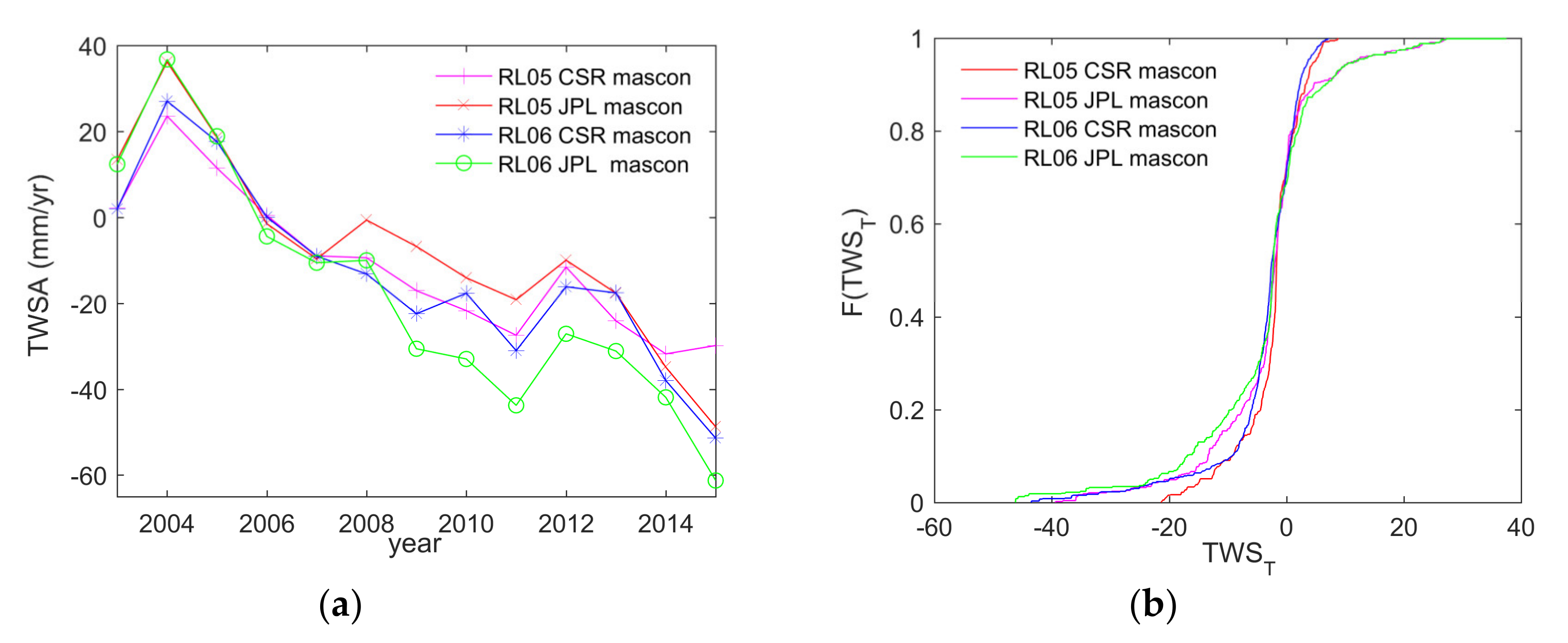
Figure 2 shows all the Mascon products of the average annual TWS anomaly (TWSA) in the UMYRC and the cumulative distribution function of trend slopes on the grid. Evidently, all Mascon products showed an agreed downward trend and the trend slopes ranged from 3.8 mm/year to 6.6 mm/year, in which the slope of RL06 JPL data was the largest and RL05 CSR data was the smallest (Figure 2a). As Figure 2b shows, when the trend slopes ranged from −2.8 mm/year to 1.6 mm/year, the cumulative distribution functions were almost the same. This indicated that the grids from different Mascon products accounted for a similar proportion in the UMYRC, with the slope range mentioned above. Yet, when the slope was greater than 1.6 mm/year (or smaller than −2.8 mm/year), the difference between the functions of different products became larger. This indicated that the spatial distribution of the products with a large trend slope was different. Considering the lack of measured values and subjective selection errors, we took the arithmetic mean of all Mascon products as the basis for later analysis in this study.

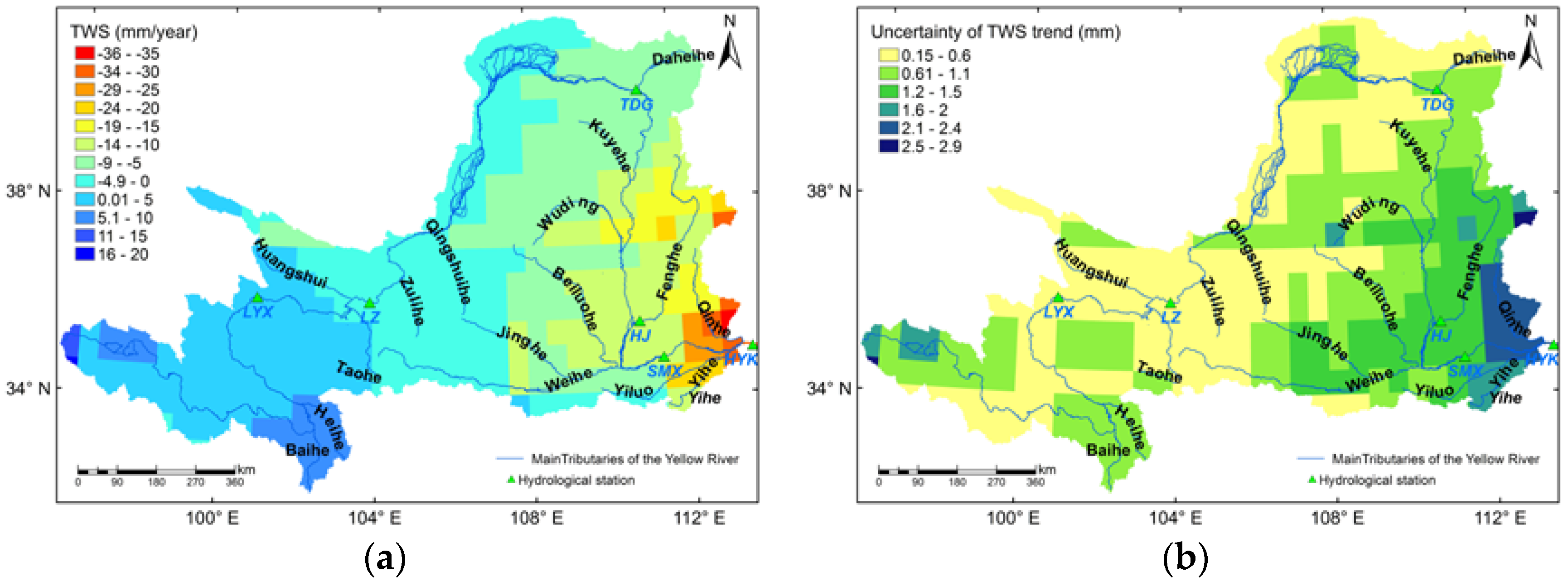
We used Sen’s slope to calculate the trend slope of TWS and other variables on the grid scale, and then mapped the trends using ArcGIS software with information about tributaries added, which are shown in Figure 3a, Figure 4, and Figure 5. The spatial variations in the trend slope of the TWS display a clear spatial pattern: the slope decreased from west to east. In addition, the TWS increased in the area above Lanzhou station (LZ) and decreased in other areas, with a large increase in TWS in the Heihe River Basin and Baihe River Basin and a significant decrease in the Qinhe River Basin and Yiluo River Basin (Figure 3a). Figure 3b shows the standard deviation for the trend slope of the TWS, where the spatial pattern corresponds to the trend slope. The uncertainty of the trend slope increased from the upper reaches to the lower. Furthermore, a larger trend was accompanied by greater uncertainty, and the largest uncertainty was in the Qinhe River Basin.

3.2. Spatial Trend Variations of Influencing Factors

In this study, the impact factors of TWS variations were precipitation (P), evapotranspiration (ET), runoff (Rs), base flow (Rsb), maximum temperature (Tmax), minimum temperature (Tmin), net radiation (NetRad), vegetation normalization index (NDVI), and human water use. Before investigating the relationships between the factors and TWS variations, we analyzed the spatial distribution characteristics of the trend slopes of each influencing factor.

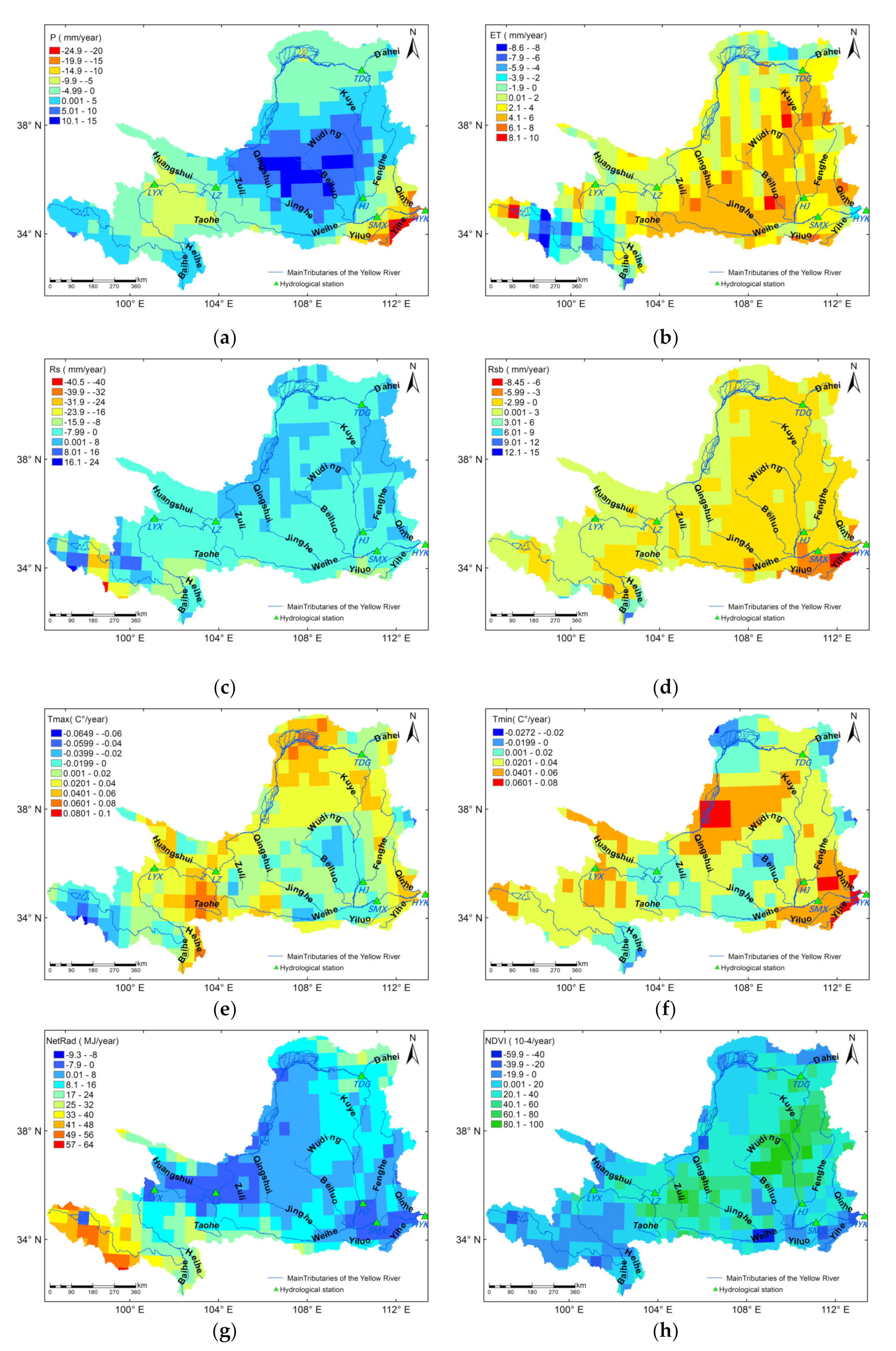
The spatial variations in the trend slope of hydro-climatic factors are shown in Figure 4a–g. The spatial distribution of the trend slope of P presented an obvious clustering feature, with increasing P mainly in the center of the Loess Plateau (Figure 4a). The spatial distributions of Tmax and Tmin were characterized by an increasing trend across the UMYRC (Figure 4e,f). The spatial distribution of the NetRad trend, which increased in the area below the SMX (Figure 4g), disagreed with that of Tmin and Tmax. Therefore, it can be concluded that the regions of the increase in water and heat in the UMYRC were inconsistent, and the impact of Tmin and Tmax on NetRad was weak.

NDVI, representing vegetation growth and vegetation coverage, was used as a factor of ecosystems in this study. Theoretically, vegetation has two-way effects on TWS, which enhances water storage by increasing the capacity of soil water storage and consumes water storage by precipitation interception and transpiration. Figure 4h shows the spatial distribution of NDVI trends, which decreased in areas above the LZ and increased in the center of the Loess Plateau. The largest increase in NDVI was in the Zhulihe River Basin and the area between the TDG and SMX. The spatial pattern of the ET trend was consistent with that of NDVI (Figure 4b) and was characterized by an increase across the UMYRC. This suggests that vegetation has a key influence on ET in the UMYRC. The trends of Rs and Rsb had similar spatial characteristics, which decreased across the UMYRC. However, differences still existed, such as the greatest decrease in Rs in the Anemaqen region and of Rsb in the Yiluo River Basin (Figure 4c,d). Furthermore, the spatial distribution of the decreasing trend of Rsb was similar to that of NDVI and ET, indicating that decreasing Rsb responded to changes in NDVI and ET.

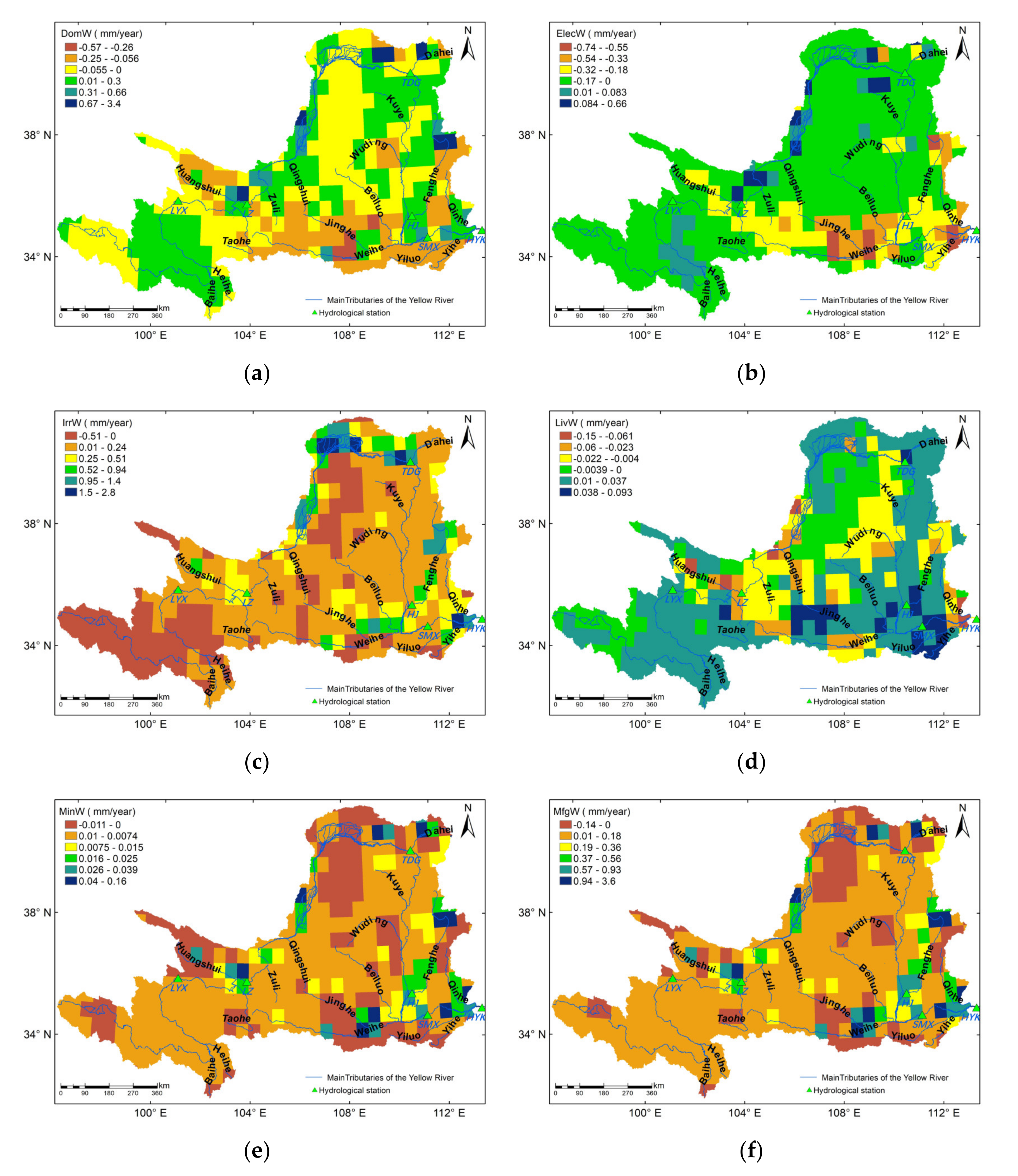
Figure 5 shows the spatial distributions of the trend slope for human water use from different sectors, which presented different spatial variation characteristics. Domestic water withdrawal (DomW) decreased in the majority of the UMYRC, with the largest reduction in the southern part of the Weihe River Basin (Figure 5a). Electricity water withdrawal (ElecW) decreased significantly in the south of the Weihe River Basin and the areas between the SMX and HYK (Huayuankou station), and it only increased in some grids along the river (Figure 5b). Irrigation water withdrawal (IrrW) increased significantly in the major irrigation areas, such as the Ningxia Irrigation Area and Hetao Irrigation District (Figure 5c). The areas where livestock water withdrawal (LivW) increased were mainly in the Weihe River Basin, and the areas above the LZ and between the SMX and HYK (Figure 5d). Compared with the others, the trend slope of mining water withdrawal (MinW) was the smallest, and the increase appeared only in larger cities along the Yellow River, such as the cities of Zhongwei, Yinchuan, Ordos, Xi’an, and Taiyuan (Figure 5e). The spatial trend of manufacturing water withdrawal (MfgW) was identical to that of MinW (Figure 5f).

3.3. Correlation between Variables

To explore the spatiotemporal relationships between variables, we calculated the Pearson’s correlation coefficients between the TWS and influencing factors on the grid trend slopes. Figure 6 shows a diagram of the correlation coefficient matrix, where red and blue indicate negative correlation and positive correlation, and a deeper color indicates a stronger correlation. In addition, the significance of the variable correlation coefficients was tested. Except for NetRad and LivW, the correlations between the remaining factors and TWS passed the significance test (P = 0.05). Moreover, TWS was negatively correlated with ET, NDVI, Tmin, IrrW, MinW, and MfgW, and positively correlated with Rsb and ElecW, with the absolute value of the correlation coefficient being greater than 0.3. Moreover, Tmin had the strongest negative correlation with TWS, and ElecW had the strongest positive correlation with TWS across the UMYRC.

Figure 6 also shows the correlation coefficients of the influencing factors on the grid trend slope. The correlations between hydro-climatic factors were all statistically significant, and the interactive directions were inconsistent. Tmin was significantly correlated with other hydro-climatic variables, which negatively correlated with Rs, Rsb, and P. Moreover, P was significantly correlated with other variables except NetRad, of which Rsb was the most relevant. Meanwhile, hydro-climatic factors affected both vegetation and human water use. For example, NDVI was positively correlated with P, ET, temperature, and NetRad, and MinW was positively correlated with Tmin. It is worth noting that different hydro-climatic factors generated opposite impacts on human water use. For example, ElecW was significantly negatively correlated with Tmin and ET, and positively correlated with Rsb. In addition, IrrW was negatively correlated with P and Rsb, and positively correlated with Tmax and Tmin. Consequently, a significant interaction process existed among the influencing factors, which may have affected the variations in TWS.

3.4. Variables and Their Interactions Identified by MARS

To avoid the uncertainty of subjective choice, this study retained all influencing factors as model inputs and allowed the MARS model to automatically identify statistically significant factors and pairs of interactive variables. The MARS model retained six variables: P, Rs, Rsb, NDVI, ElecW, and Tmin, which constituted 15 basic equations (excluding intercept) consisting of four univariate influencing functions and five multivariate influencing functions. The MAE and GCV of the final model were 1.18 mm and 5.2 mm, respectively.

Table 2. A list of the variables retained by MARS and their corresponding basic equations with coefficient and node value.

Basis	Coefficient	P	Rs	Rsb	NDVI	ElecW	Tmin
Function
1	−0.35					1(0)
2	−0.48					−1(0)
3	−0.90	−1(−1.47)
4	4.70			1(−2.32)
5	2.90			−1(−2.32)
6	−835.68				1(−0.000755)
7	0.51		1(1.95)			−1(0)
8	0.06		−1(1.95)			−1(0)
9	−770.94		1(−0.27)		1(−0.000755)
10	243.01		−1(−0.27)		1(−0.000755)
11	0.32	1(−1.47)	1(−1.89)
12	−0.26	1(−7.30)		1(−2.32)
13	−0.58	−1(−7.30)		1(−2.32)
14	−13.56					−1(0)	1(0.0145)
15	−48.13					−1(0)	−1(0.0145)

Each row represents a MARS term in which the factor having 1 indicates the form (x − t)₊ (i.e, x > t), −1 indicates the form (t − x)₊ (i.e., x < t).

lists 15 basic equations (BF), their corresponding coefficients, and the node positions shown in brackets.

Figure 7a–d depict the impact of the trend slopes for single variables identified by MARS on TWS variations. The line in Figure 7 represents the single variable function as shown in Table 2 (BF1–BF6), and the scatter plot is the relationship for the grid trend slopes between the single variable and TWS calculated from GRACE. According to the MARS model, ElecW, P, Rsb, and NDVI had a significant effect on the variations in TWS across the UMYRC. Within the grids for the study area, the trend slope change of ElecW and Rsb was inconsistent with that of TWS, which indicated that the impact of ElecW and Rsb on TWS existed in two ways (Figure 7a,c). When the slope of ElecW was negative and the slope of Rsb was greater than −2.32 mm/year, the increase in trend for the variables enhanced the slope of TWS, which occurred in most areas of the basin (Figure 5b and Figure 4d). In the Baihe River Basin and Heihe River Basin, the increasing trend of Rsb attenuated the trend of TWS. In the center of the Loess Plateau, where the slope of P was greater than −1.47 mm/year, the impact of P on TWS was slight. However, in the middle part of the source area and the section from the SMX to HYK, the decreasing slope of P reduced the slope of the TWS (Figure 4a and Figure 7b). At the same time, the trend of NDVI also had a different impact on the trend of TWS. The increase in the NDVI trend weakened the slope of TWS in the Loess Plateau when the slope was greater than 0.000755, with little contribution to the TWS trend in the area above the LZ (Figure 7d and Figure 4h).

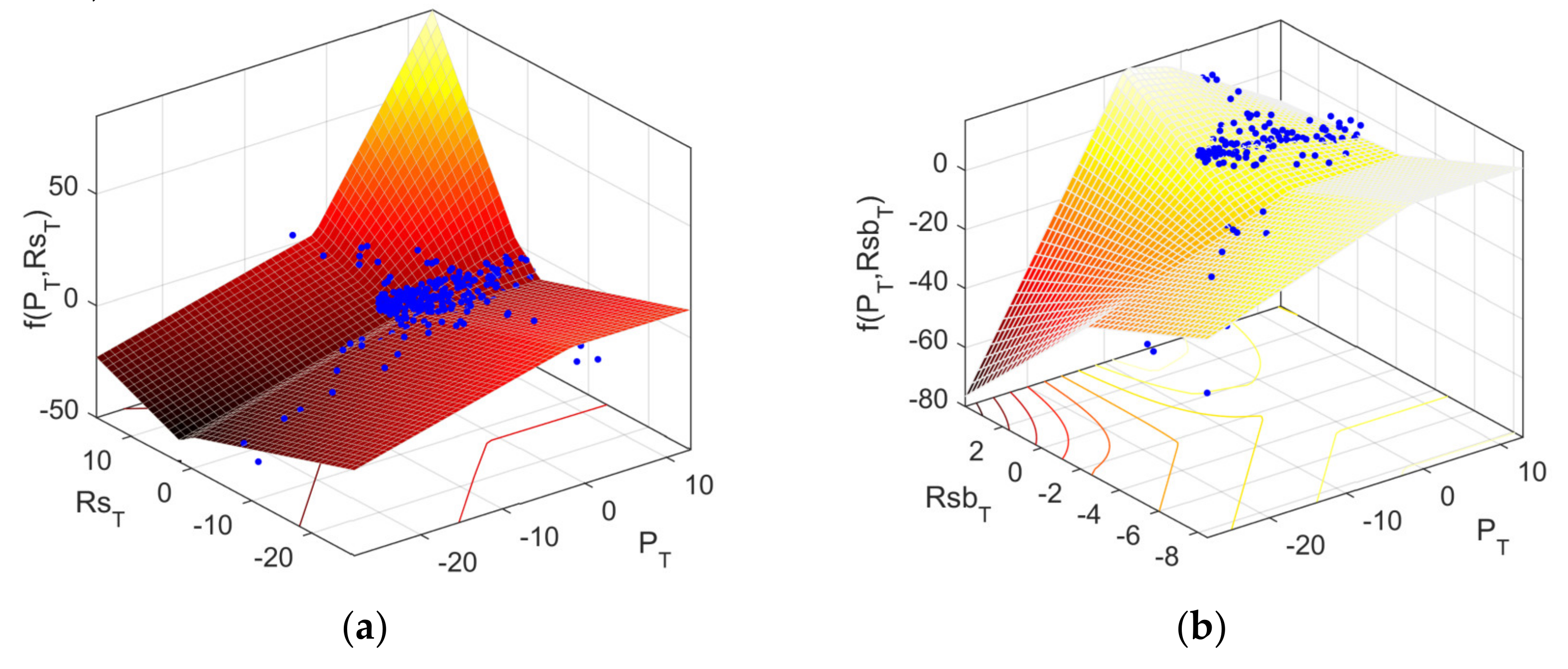
Figure 8a–e show the influence of multivariable synergy on the trend slope of TWS. The curved surface in Figure 8 was estimated by synergetic variables using the final model, with other variables fixed at the middle of their ranges. Moreover, the scatter plot shows the relationship between the trend slopes of the synergetic variable pair and the TWS calculated from GRACE. Five pairs of synergetic variables identified by MARS were P and Rs, P and Rsb, ElecW and Tmin, NDVI and Rs, and ElecW and Rs. The interactions of variable pairs on the TWS trend varied across the study area. On the condition that the slope of P and Rs outnumbered −1.47 mm/year and −1.89 mm/year, the interaction for P and Rs increased the TWS in the middle of the Loess Plateau (Figure 8a, Figure 4a, and Figure 4c), while the area where the slope of Rsb and P outnumbered −2.32 mm/year and −7.3 mm/year, where both variables worked together to decrease the trend of TWS, was mainly in the region above the HJ (Figure 8b). Moreover, the interaction of Rs with ElecW or NDVI altered the effect on the trend slope of TWS, compared with the action of ElecW or NDVI alone. In the middle of the Loess Plateau, where the trend of Rs and ElecW was, respectively, less than 1.95 mm/year and zero, the interaction between Rs and ElecW decreased the trend of TWS (Figure 8d). Further, in the Yihe River Basin and Yiluo River Basin, the trend slope for NDVI and Rs was, respectively, less than 0.000755 and −0.27 mm/year, and the interplay of variables reduced the trend of TWS (Figure 8c). The last interactive variables were Tmin and ElecW, which diminished the trend of TWS in the area where the trends of ElecW and Tmin were lower than zero and 0.0145 C°/year (Figure 8e).

Concurrently, we also estimated the relative importance of univariate and multivariate functions in the MARS model using ANOVA (Figure 9). As shown in Figure 9, Rsb had the greatest influence on the trend of TWS, followed by P. The most important effects of multivariate synergy were P and Rs, followed by Rs and NDVI.

3.5. Assessment of MARS Model’s Performance

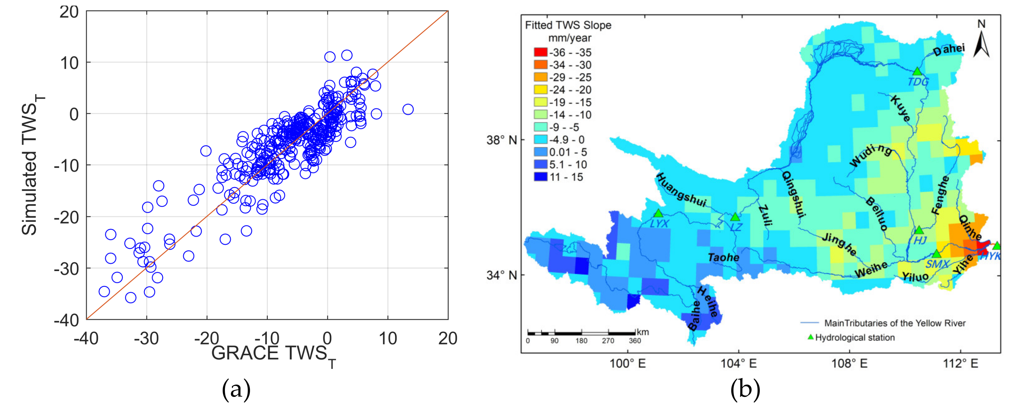
Figure 10a compares the trend of TWS estimated by the MARS model and calculated from the GRACE data. The simulated values of the grid trend agreed well with the measured values, with a determination coefficient (R²) of 0.83 and a mean absolute error (MAE) of 1.18 mm. Figure 10b shows the spatial distribution of trend slopes for TWS assessed by the MARS model, which resembled the spatial distribution pattern of TWS shown in Figure 3a. Therefore, the MARS model can explain the spatiotemporal variations in TWS well, and it is credible to use the MARS model to identify the main driving factors and their interactions on the variations in TWS across the UMYRC.

In addition, the input variables for the MARS model were divided into three groups, and the fitting results of various models were compared based on the determination coefficient (R²), mean absolute error (MAE), and Akachi information criterion (AIC). In addition, there are two interactive variables for all the models, and the maximum number of basic equations for the forward phase was set as mentioned earlier. The evaluation indexes of the regression model based on the input variables of the four groups for the MARS model are listed in

Table 3. List of fitting results of different input variables.

Category	Input Variables	R2	MAE	AIC
1	P, ET, Rs, Rsb	0.65	1.84	2381.94
2	DomW, ElecW, MinW, LivW, IrrW, MfgW	0.66	1.70	2371.30
3	NDVI, Tmin, Tmax, NetRad	0.56	1.88	2631.62
4	All factors	0.83	1.18	1702.66

. The evaluation indexes (R² and MAE) of models for input variables of categories one to three were all lower than the total variable model. In addition, the AIC values of the models for categories one to three were all higher than the total variable model. Therefore, the total variable model (category four) can better explain the spatiotemporal variations in TWS than other categories.

4. Discussion

4.1. Main Influencing Factors of TWS Spatiotemporal Variations

Our study found that six variables significantly affected the spatiotemporal variations in TWS: Rsb, NDVI, ElecW, P, Rs, and Tmin. Among these variables, Rs and Tmin played an important role in the variations in TWS only when they cooperated with other variables. In this section, we discuss only the variables that directly affected TWS significantly. The P and Rsb of hydro-climatic factors were the main driving factors for the spatiotemporal variations in TWS in the UMYRC. The decreased P was the major factor for the decreased TWS in the Fenhe River Basin, north of the inner basin, Hetao Irrigation District, and the area between the SMX and HYK. The decreased Rsb was the reason for the decreased TWS in the Loess Plateau, and for the increased TWS in the area from west of Anemaqen to Lake Zaling and the area between LYX and LZ. Nevertheless, previous studies have shown that groundwater storage declined in the Yellow River Basin [36].

Because of the Policy of Returning Cultivated Land to Forest, Grassland and Ecological Afforestation, the vegetation in this study area has turned green significantly [22], and many studies [62,63,64] have shown that the water consumption function of vegetation in arid and semi-arid areas surpasses that of water storage. Our results also indicated that the function of water consumption of vegetation dominated in the Loess Plateau, which is consistent with the results of previous studies. Additionally, the increased NDVI was the main factor affecting the decreased TWS in the Loess Plateau.

In human water use of different departments, ElecW was the main factor affecting the spatial variations in the TWS trend. Thermal power generation is the main power supply in the Yellow River Basin, accounting for 80% of the total power generation [65]. The area of ElecW reduction accounted for 91% of the study area, so the decreased ElecW was the main factor of TWS spatial change. Moreover, the decreased ElecW was the driver for the increased TWS of the source region, except for the area between the Baihe River and the LYX, and the increased ElecW was responsible for the decreased TWS in the Yinchuan Plain and Hetao Irrigation District.

4.2. Impact of Factors’ Interaction on Spatiotemporal Variations in TWS

We identified five pairs of interactive variables affecting the TWS variations: P with Rs and Rsb, ElecW and Tmin, ElecW and Rs, and Rs and NDVI. The synergies suggested that although the direct influence of variables on TWS was not significant, its indirect impact with other significant variables could not be ignored. Moreover, the synergy could alter the way and intensity of a single variable for the effect on TWS variations. For example, under the condition that the trend slope of ElecW was negative, when the trend of Tmin exceeded 0.0145 C°/year and the trend of Rs was lower than 1.95 mm/year, the impact of ElecW on the TWS trend changed from increasing to decreasing. The interaction between ElecW and Tmin primarily characterized the influence of Tmin on ElecW. Tmin always arises in winter, when other forms of energy (water and solar) are decreased, and ElecW is negatively correlated with Tmin. The lower the Tmin, the greater the need for ElecW. In addition, the study found that the synergy of ElecW and Tmin was the reason for the increased TWS in the Baihe River Basin and the Heihe River Basin, and the decreased TWS in the Qingshui River Basin, Kuye River Basin, Wuding River Basin, and the area between the HJ and HYK.

The main power supply modes in the Yellow River Basin are hydropower affected by runoff and thermal power generation, which work together to meet electricity needs. Therefore, the impact of Rs on ElecW is actually a balance between the proportion of hydropower generation and thermal power generation, and the interaction of ElecW and Rs reflects the dependence of electric energy, the basis of social and economic development, on water resources in the Yellow River Basin. In addition, the synergy of ElecW and Rs was the reason for the increased TWS in the area of Lake Zaling and Eling and Anemaqen, and for the decreased TWS in the area between the middle of the Loess Plateau.

Vegetation, a key component of terrestrial ecosystems, affects surface runoff and underground runoff by enhancing soil infiltration capacity. Meanwhile, it consumes soil water and groundwater through transpiration and interception. Therefore, the interaction between NDVI and Rs mainly implies the effect of NDVI on Rs, and the interactive process reflects the interconnection between ecology and hydrology. Our study found that the interaction of Rs and NDVI decreased the TWS trend, on the condition that the trend of NDVI and the Rs trend outweighed −0.000755 and −0.27 mm/ year, respectively. In addition, the synergy of NDVI and Rs was the reason for the decreased TWS in the Yinchuan Plain, Mu Us Desert, the north of the Hetao Irrigation District, and upstream of the Fenhe River Basin, and the increased TWS upstream of the UMYRC.

The synergetic effect of P with Rs and Rsb on TWS states the relationship between precipitation and the runoff process and water storage change in hydrological systems [66]. When the trends for P and Rs outnumbered −1.47 mm/year and −1.89 mm/year, the two variables worked together to increase the TWS trend. The results also suggested that the response of TWS to precipitation and runoff was delayed, which reflects the stability and adaptability of the hydrological system. Moreover, the synergy of P and Rs was the reason for the increased TWS in the areas of Lake Eling and Lake Zaling. At the same time, on the condition that the trend of Rsb and P outnumbered −2.32 mm/year and −7.3 mm/year, the impact of the two variables on the trend of TWS altered from diminishing to enhancing. In the Heihe River Basin and the Baihe River Basin and west of the source area, the increased P and Rsb were the main factors for the increase in TWS. In the section from the SMX to HYK, the decrease in P and Rsb led to a decrease in TWS.

4.3. Uncertainty and Limitations

In this study, the effects of 14 variables from hydrological climate, vegetation, and human activities and their synergistic effect on TWS variations were investigated in the UMYRC. The inclusion of more influencing factors can eliminate the problem of biased sampling and reduce model uncertainty [46]. While the interaction may occur among more variables, there were two interactive variables in this study, which can cause a potential error when using the MARS model to discern synergies on TWS variations. To assess the effect of the number of interactive variables on the final model, we also set a different number of those for the fitting model, and found that the drivers and interactions identified by MARS were the same. Compared with previous studies, this study investigated the impact of spatial variation and the interaction of variables on spatiotemporal variations in TWS, providing an effective mode for the study of spatiotemporal variations in TWS. Moreover, the internal mechanism of variable interactions on the effect of TWS variations is not clear; thus, it is necessary to combine the models from different systems such as hydrology, ecology, and energy in future research.

5. Conclusions

TWS variations are driven by the joint actions of climate and human activities, and there are multiple interactive processes among various factors. The interaction contains certain physical processes that help expound the mechanism for TWS variations from the perspective of different subsystems. This study used trends of climate, human water use, and vegetation derived from multi-source data to investigate the drivers and their synergy for spatial variations in TWS trends during 2003–2015 by MARS.

The trend rate of TWS estimated by GRACE increased from east to west in the UMYRC, and TWS increased in the upper reaches of the LZ and decreased in the lower reaches. The spatial distributions of the influencing factors of TWS variations were significantly different. The analysis of the correlation coefficient indicated that the spatial distribution of the TWS trend was significantly associated with the spatial variations in the trends of ET, Rsb, Tmin, NDVI, ElecW, IrrW, and MfgW. Meanwhile, there were significant connections between factors from hydro-climatic and human water use, such as ElecW and Tmin, IrrW, and P.

The grid rate of TWS evaluated from the MARS model agreed well with that estimated from GRACE, with a determined coefficient (R²) of 0.83 and a root mean square error (MAE) of 1.2 mm. Moreover, the spatial distributions of trends derived from the MARS model and GRACE data were similar. The MARS model identified that Rs, ElecW, NDVI, Rsb, P, and Tmin were statistically significant factors that dominated the variation in the TWS trend across the UMYRC. Among the determinants, the contribution of Rsb was the largest and Tmin was the smallest. Apart from the effect of a single factor, there were five pairs of interactive variables driving the variations in TWS, which were ElecW with Tmin and Rs, NDVI and Rs, P with Rs and Rsb. Among the interactive variables, the synergistic effect of P and Rsb contributed the most to the spatial variations in the TWS trend, followed by Rs and NDVI.

The key factors affecting the change in TWS in different regions of the UMYRC are as follows. The increase in Rsb, ElecW, and the interaction between NDVI and Rs were the reasons for the increased TWS in the area above Lanzhou station. At the same time, the synergistic effect of ElecW and Tmin in the Heihe River Basin and Baihe River Basin and the synergistic effect of P and Rs in the Zaling and Eling Lake regions were also important. The drivers for the decrease in TWS in the Loess Plateau were the increase in NDVI, the decrease in Rsb, and the synergy of ElecW and Rs. Furthermore, the synergy of NDVI and Rs and the reduction in P were the decisive factors for TWS change in the Fenhe River Basin, Hetao Irrigation District, and internal flow area. Additionally, the interactions between ElecW and Tmin, P and Rsb were the driving forces for the reduced TWS in the regions from the SMX to HYK.

Overall, we thought that the TWS change in the UMYRC resulted from the coupling effect of the water energy system, eco-hydrological system, and hydrological system. Therefore, the balanced distribution of water among different systems will alleviate the contradiction of water resources in the Yellow River Basin. Furthermore, the hydrological system plays the most important role in the change in terrestrial water resources, and the relationships of precipitation–runoff and runoff–water storage are the key processes in the hydrological system.

References

1. Guentner, A.; Stuck, J.; Werth, S.; Doell, P.; Verzano, K.; Merz, B. A Global Analysis of Temporal and Spatial Variations in Continental Water Storage. Water Resour. Res. 2007, 43, 687–6906. [Google Scholar] [CrossRef]
2. Riegger, J. Quantification of Drainable Water Storage Volumes in Catchments in River Networks on Global Scales Using the GRACE and/or River Runoff. Hydrol. Earth Syst. Sci. Discuss. 2018, 1–27. [Google Scholar] [CrossRef]
3. Joodakii, G.; Wahr, J.; Swenson, S. Estimating the Human Contribution to Groundwater Depletion in the Middle East, from GRACE Data, Land Surface Models, and Well Observations. Water Resour. Res. 2014, 50, 2679–2692. [Google Scholar] [CrossRef]
4. Girotto, M.; Rodell, M. Terrestrial water storage. In Extreme Hydroclimatic Events and Multivariate Hazards in a Changing Environment; Elsevier: Amsterdam, The Netherlands, 2019; pp. 41–64. ISBN 978-0-12-814899-0. [Google Scholar]
5. Ahmed, M.; Sultan, M.; Wahr, J.; Yan, E. The Use of GRACE Data to Monitor Natural and Anthropogenic Induced Variations in Water Availability across Africa. Earth-Sci. Rev. 2014, 136, 289–300. [Google Scholar] [CrossRef]
6. Wahr, J.; Molenaar, M.; Bryan, F. Time Variability of the Earth’s Gravity Field: Hydrological and Oceanic Effects and Their Possible Detection Using GRACE. J. Geophys. Res. Solid Earth 1998, 103, 30205–30229. [Google Scholar] [CrossRef]
7. Wahr, J.; Swenson, S.; Zlotnicki, V.; Velicogna, I. Time-Variable Gravity from GRACE: First Results. Geophys. Res. Lett. 2004, 31, 293–317. [Google Scholar] [CrossRef] [Green Version]
8. Swenson, S.; Yeh, P.J.-F.; Wahr, J.; Famiglietti, J. A Comparison of Terrestrial Water Storage Variations from GRACE with in Situ Measurements from Illinois. Geophys. Res. Lett. 2006, 33. [Google Scholar] [CrossRef] [Green Version]
9. Rodell, M.; Chen, J.; Kato, H.; Famiglietti, J.S.; Nigro, J.; Wilson, C.R. Estimating Groundwater Storage Changes in the Mississippi River Basin (USA) Using GRACE. Hydrogeol. J. 2007, 15, 159–166. [Google Scholar] [CrossRef] [Green Version]
10. Grippa, M.; Kergoat, L.; Frappart, F.; Araud, Q.; Boone, A.; de Rosnay, P.; Lemoine, J.-M.; Gascoin, S.; Balsamo, G.; Ottlé, C.; et al. Land Water Storage Variability over West Africa Estimated by Gravity Recovery and Climate Experiment (GRACE) and Land Surface Models. Water Resour. Res. 2011, 47. [Google Scholar] [CrossRef]
11. Nakaegawa, T.; Yamamoto, K.; Tanaka, T.Y.; Hasegawa, T.; Fukuda, Y. Investigation of Temporal Characteristics of Terrestrial Water Storage Changes and Its Comparison to Terrestrial Mass Changes. Hydrol. Process. 2012, 26, 2470–2481. [Google Scholar] [CrossRef]
12. Yang, P.; Xia, J.; Zhan, C.; Qiao, Y.; Wang, Y. Monitoring the Spatio-Temporal Changes of Terrestrial Water Storage Using GRACE Data in the Tarim River Basin between 2002 and 2015. Sci. Total Environ. 2017, 595, 218–228. [Google Scholar] [CrossRef]
13. Chen, H.; Liu, H.; Chen, X.; Qiao, Y. Analysis on Impacts of Hydro-Climatic Changes and Human Activities on Available Water Changes in Central Asia. Sci. Total Environ. 2020, 737, 139779. [Google Scholar] [CrossRef] [PubMed]
14. Syed, T.H.; Famiglietti, J.S.; Chen, J.; Rodell, M.; Seneviratne, S.I.; Viterbo, P.; Wilson, C.R. Total Basin Discharge for the Amazon and Mississippi River Basins from GRACE and a Land-Atmosphere Water Balance. Geophys. Res. Lett. 2005, 32. [Google Scholar] [CrossRef] [Green Version]
15. Wang, S.; Huang, J.; Li, J.; Rivera, A.; McKenney, D.W.; Sheffield, J. Assessment of Water Budget for Sixteen Large Drainage Basins in Canada. J. Hydrol. 2014, 512, 1–15. [Google Scholar] [CrossRef]
16. Rodell, M. Basin Scale Estimates of Evapotranspiration Using GRACE and Other Observations. Geophys. Res. Lett. 2004, 31. [Google Scholar] [CrossRef] [Green Version]
17. Xiaoyu, S.; Caiping, J.; Bing, S.; Wenjuan, S.; Lingmei, H. Interaction between ecological environment construction and sustainable use of water resources in Northwest China. Agric. Res. Arid Areas 2004, 22, 127–131. [Google Scholar]
18. Wada, Y.; van Beek, L.P.H.; van Kempen, C.M.; Reckman, J.W.T.M.; Vasak, S.; Bierkens, M.F.P. Global Depletion of Groundwater Resources. Geophys. Res. Lett. 2010, 37. [Google Scholar] [CrossRef] [Green Version]
19. Yin, Y.; Tang, Q.; Liu, X.; Zhang, X. Water Scarcity under Various Socio-Economic Pathways and Its Potential Effects on Food Production in the Yellow River Basin. Hydrol. Earth Syst. Sci. 2017, 21, 791–804. [Google Scholar] [CrossRef] [Green Version]
20. Ya, L.; Shengtian, Y.; Xiaoyan, L.; Changming, L.; Wenlong, S.; Guotao, D.; Haigen, Z.; Hezhen, L. Land Use Change in the Reach from Hekouzhen to Tongguan of the Yellow River during 1998–2010. Acta Geogr. Sin. 2014, 69, 42–53. [Google Scholar]
21. Guangqian, W.; Siyuan, W.; Zhixiang, C. Land-use/land-cover changes in the Yellow River basin. J. Tsinghua Univ. (Sci. Technol.) 2004, 44, 1218–1222. [Google Scholar]
22. Kong, D.; Miao, C.; Borthwick, A.G.L.; Lei, X.; Li, H. Spatiotemporal Variations in Vegetation Cover on the Loess Plateau, China, between 1982 and 2013: Possible Causes and Potential Impacts. Environ. Sci. Pollut. Res. 2018, 25, 13633–13644. [Google Scholar] [CrossRef] [PubMed] [Green Version]
23. Dawen, Y.; Shulei, Z.; Xiangyu, X. Attribution analysis for runoff decline in Yellow River Basin during past fifty years based on Budyko hypothesis. Sci. Sin. 2015, 45, 1024–1034. [Google Scholar] [CrossRef] [Green Version]
24. Zuo, D.; Xu, Z.; Yao, W.; Jin, S.; Xiao, P.; Ran, D. Assessing the Effects of Changes in Land Use and Climate on Runoff and Sediment Yields from a Watershed in the Loess Plateau of China. Sci. Total Environ. 2016, 544, 238–250. [Google Scholar] [CrossRef] [PubMed]
25. Jia, X.; Shao, M.; Zhu, Y.; Luo, Y. Soil Moisture Decline Due to Afforestation across the Loess Plateau, China. J. Hydrol. 2017, 546, 113–122. [Google Scholar] [CrossRef]
26. Zhang, K.; Xie, X.; Zhu, B.; Meng, S.; Yao, Y. Unexpected Groundwater Recovery with Decreasing Agricultural Irrigation in the Yellow River Basin. Agric. Water Manag. 2019, 213, 858–867. [Google Scholar] [CrossRef]
27. Sun, W.; Jin, Y.; Yu, J.; Wang, G.; Xue, B.; Zhao, Y.; Fu, Y.; Shrestha, S. Integrating Satellite Observations and Human Water Use Data to Estimate Changes in Key Components of Terrestrial Water Storage in a Semi-Arid Region of North China. Sci. Total Environ. 2020, 698, 134171. [Google Scholar] [CrossRef]
28. Lv, M.; Ma, Z.; Li, M.; Zheng, Z. Quantitative Analysis of Terrestrial Water Storage Changes Under the Grain for Green Program in the Yellow River Basin. J. Geophys. Res. Atmos. 2019, 124, 1336–1351. [Google Scholar] [CrossRef]
29. Li, C.; Zhang, Y.; Shen, Y.; Yu, Q. Decadal Water Storage Decrease Driven by Vegetation Changes in the Yellow River Basin. Sci. Bull. 2020, 65, 1859–1861. [Google Scholar] [CrossRef]
30. Xie, J.; Xu, Y.-P.; Wang, Y.; Gu, H.; Wang, F.; Pan, S. Influences of Climatic Variability and Human Activities on Terrestrial Water Storage Variations across the Yellow River Basin in the Recent Decade. J. Hydrol. 2019, 579, 124218. [Google Scholar] [CrossRef]
31. Jing, W.; Yao, L.; Zhao, X.; Zhang, P.; Liu, Y.; Xia, X.; Song, J.; Yang, J.; Li, Y.; Zhou, C. Understanding Terrestrial Water Storage Declining Trends in the Yellow River Basin. J. Geophys. Res. Atmos. 2019, 124, 12963–12984. [Google Scholar] [CrossRef]
32. Deng, H.; Pepin, N.C.; Liu, Q.; Chen, Y. Understanding the Spatial Differences in Terrestrial Water Storage Variations in the Tibetan Plateau from 2002 to 2016. Clim. Chang. 2018, 151, 379–393. [Google Scholar] [CrossRef] [Green Version]
33. Wang, J.; Chen, X.; Hu, Q.; Liu, J. Responses of Terrestrial Water Storage to Climate Variation in the Tibetan Plateau. J. Hydrol. 2020, 584, 124652. [Google Scholar] [CrossRef]
34. Meng, F.; Su, F.; Li, Y.; Tong, K. Changes in Terrestrial Water Storage During 2003–2014 and Possible Causes in Tibetan Plateau. J. Geophys. Res. Atmos. 2019, 124, 2909–2931. [Google Scholar] [CrossRef]
35. Chen, X.; Jiang, J.; Lei, T.; Yue, C. GRACE Satellite Monitoring and Driving Factors Analysis of Groundwater Storage under High-Intensity Coal Mining Conditions: A Case Study of Ordos, Northern Shaanxi and Shanxi, China. Hydrogeol. J. 2020, 28, 673–686. [Google Scholar] [CrossRef]
36. Xie, X.; Xu, C.; Wen, Y.; Li, W. Monitoring Groundwater Storage Changes in the Loess Plateau Using GRACE Satellite Gravity Data, Hydrological Models and Coal Mining Data. Remote Sens. 2018, 10, 605. [Google Scholar] [CrossRef] [Green Version]
37. Yi, S.; Song, C.; Wang, Q.; Wang, L.; Heki, K.; Sun, W. The Potential of GRACE Gravimetry to Detect the Heavy Rainfall-Induced Impoundment of a Small Reservoir in the Upper Yellow River. Water Resour. Res. 2017, 53, 6562–6578. [Google Scholar] [CrossRef]
38. Wang, X.; Zhang, J.; Shamsuddin, S.; Oyang, R.; Guan, T.; Xue, J.; Zhang, X. Impacts of Climate Variability and Changes on Domestic Water Use in the Yellow River Basin of China. Mitig. Adapt. Strat. Strateg. Glob. Chang. 2017, 22, 595–608. [Google Scholar] [CrossRef]
39. Wang, X.; Zhang, J.; Shahid, S.; Guan, E.; Wu, Y.; Gao, J.; He, R. Adaptation to Climate Change Impacts on Water Demand. Mitig. Adapt. Strateg. Glob. Chang. 2016, 21, 81–99. [Google Scholar] [CrossRef]
40. Ellison, D.; Morris, C.E.; Locatelli, B.; Sheil, D.; Cohen, J.; Murdiyarso, D.; Gutierrez, V.; van Noordwijk, M.; Creed, I.F.; Pokorny, J.; et al. Trees, Forests and Water: Cool Insights for a Hot World. Glob. Environ. Chang. Hum. Policy Dimens. 2017, 43, 51–61. [Google Scholar] [CrossRef]
41. Lin, M.; Biswas, A.; Bennett, E.M. Socio-Ecological Determinants on Spatio-Temporal Changes of Groundwater in the Yellow River Basin, China. Sci. Total Environ. 2020, 731, 138725. [Google Scholar] [CrossRef]
42. Hasan, E.; Tarhule, A. GRACE: Gravity Recovery and Climate Experiment Long-Term Trend Investigation over the Nile River Basin: Spatial Variability Drivers. J. Hydrol. 2020, 586, 124870. [Google Scholar] [CrossRef]
43. Lin, M.; Biswas, A.; Bennett, E.M. Spatio-Temporal Dynamics of Groundwater Storage Changes in the Yellow River Basin. J. Environ. Manag. 2019, 235, 84–95. [Google Scholar] [CrossRef] [PubMed]
44. Zhang, Y.; He, B.; Guo, L.; Liu, J.; Xie, X. The Relative Contributions of Precipitation, Evapotranspiration, and Runoff to Terrestrial Water Storage Changes across 168 River Basins. J. Hydrol. 2019, 579, 124194. [Google Scholar] [CrossRef]
45. Friedman, J.H. Multivariate Adaptive Regression Splines. Ann. Stat. 1991, 19, 1–141. [Google Scholar] [CrossRef]
46. Shao, Q.; Traylen, A.; Zhang, L. Nonparametric Method for Estimating the Effects of Climatic and Catchment Characteristics on Mean Annual Evapotranspiration. Water Resour. Res. 2012, 48. [Google Scholar] [CrossRef]
47. Xing, W.; Wang, W.; Shao, Q.; Yong, B. Identification of Dominant Interactions between Climatic Seasonality, Catchment Characteristics and Agricultural Activities on Budyko-Type Equation Parameter Estimation. J. Hydrol. 2018, 556, 585–599. [Google Scholar] [CrossRef]
48. Chen, J.L.; Wilson, C.R.; Tapley, B.D.; Ries, J.C. Low Degree Gravitational Changes from GRACE: Validation and Interpretation. Geophys. Res. Lett. 2004, 31, L22607. [Google Scholar] [CrossRef]
49. Save, H.; Bettadpur, S.; Tapley, B.D. Reducing Errors in the GRACE Gravity Solutions Using Regularization. J. Geod. 2012, 86, 695–711. [Google Scholar] [CrossRef]
50. Scanlon, B.R.; Zhang, Z.; Save, H.; Sun, A.Y.; Schmied, H.M.; van Beek, L.P.H.; Wiese, D.N.; Wada, Y.; Long, D.; Reedy, R.C.; et al. Global Models Underestimate Large Decadal Declining and Rising Water Storage Trends Relative to GRACE Satellite Data. Proc. Natl. Acad. Sci. USA 2018, 115, E1080–E1089. [Google Scholar] [CrossRef] [PubMed] [Green Version]
51. Huang, Z.; Yeh, P.J.-F.; Pan, Y.; Jiao, J.J.; Gong, H.; Li, X.; Güntner, A.; Zhu, Y.; Zhang, C.; Zheng, L. Detection of Large-Scale Groundwater Storage Variability over the Karstic Regions in Southwest China. J. Hydrol. 2019, 569, 409–422. [Google Scholar] [CrossRef]
52. Rodell, M.; Houser, P.R.; Jambor, U.; Gottschalck, J.; Mitchell, K.; Meng, C.-J.; Arsenault, K.; Cosgrove, B.; Radakovich, J.; Bosilovich, M.; et al. The Global Land Data Assimilation System. Bull. Am. Meteorol. Soc. 2004, 85, 381–394. [Google Scholar] [CrossRef] [Green Version]
53. Huang, Z.; Hejazi, M.; Li, X.; Tang, Q.; Vernon, C.; Leng, G.; Liu, Y.; Doell, P.; Eisner, S.; Gerten, D.; et al. Reconstruction of global gridded monthly sectoral water withdrawals for 1971–2010 and analysis of their spatiotemporal patterns. Hydrol. Earth Syst. Sci. 2018, 22, 1–30. [Google Scholar] [CrossRef] [Green Version]
54. Sun, W.; Wang, Y.; Fu, Y.H.; Xue, B.; Wang, G.; Yu, J.; Zuo, D.; Xu, Z. Spatial Heterogeneity of Changes in Vegetation Growth and Their Driving Forces Based on Satellite Observations of the Yarlung Zangbo River Basin in the Tibetan Plateau. J. Hydrol. 2019, 574, 324–332. [Google Scholar] [CrossRef]
55. Piao, S.; Wang, X.; Ciais, P.; Zhu, B.; Wang, T.; Liu, J. Changes in Satellite-Derived Vegetation Growth Trend in Temperate and Boreal Eurasia from 1982 to 2006. Glob. Chang. Biol. 2011, 17, 3228–3239. [Google Scholar] [CrossRef]
56. Kendall, M.G. Rank Correlation Methods. Brit. J. Psychol. 1990, 25, 86–91. [Google Scholar] [CrossRef]
57. Mann, H.B. Nonparametric Tests against Trend. Econometrica 1945, 13, 245–259. [Google Scholar] [CrossRef]
58. Sen, K.P. Estimates of the Regression Coefficient Based on Kendall’s Tau. J. Am. Stat. Assoc. 1968, 63, 1379–1389. [Google Scholar] [CrossRef]
59. Groemping, U. Relative Importance for Linear Regression in R: The Package Relaimpo. J. Stat. Softw. 2006, 17. [Google Scholar] [CrossRef] [Green Version]
60. Yuan, R.-Q.; Chang, L.-L.; Gupta, H.; Niu, G.-Y. Climatic Forcing for Recent Significant Terrestrial Drying and Wetting. Adv. Water Resour 2019, 133, 1103425. [Google Scholar] [CrossRef]
61. Jekabsons, G. ARESLab: Adaptive Regression Splines Toolbox for Matlab/Octave. 2016. Available online: http://www.cs.rtu.lv/jekabsons/regression.html (accessed on 25 August 2021).
62. Jia, Y.-H.; Shao, M.-A. Dynamics of Deep Soil Moisture in Response to Vegetational Restoration on the Loess Plateau of China. J. Hydrol. 2014, 519, 523–531. [Google Scholar] [CrossRef]
63. Wang, Z.; Liu, B.; Liu, G.; Zhang, Y. Soil Water Depletion Depth by Planted Vegetation on the Loess Plateau. Sci. China Ser. D 2009, 52, 835–842. [Google Scholar] [CrossRef]
64. Yang, L.; Wei, W.; Chen, L.; Chen, W.; Wang, J. Response of Temporal Variation of Soil Moisture to Vegetation Restoration in Semi-Arid Loess Plateau, China. Catena 2014, 115, 123–133. [Google Scholar] [CrossRef]
65. Ma, S.; Zhang, W. Spatial and Temporal Development Pattern and Environmentally-friendly Development Path of Electricity Industry in the Yellow River Basin. Bull. Chin. Acad. Sci. 2020, 35, 86–98. [Google Scholar] [CrossRef]
66. Zhang, L.; Karthikeyan, R.; Bai, Z.; Srinivasan, R. Analysis of Streamflow Responses to Climate Variability and Land Use Change in the Loess Plateau Region of China. Catena 2017, 154, 1–11. [Google Scholar] [CrossRef]
Figure 1. The location and elevation as well as the distribution of the main tributaries and irrigation areas of the study area. The green triangles represent the location of hydrological sites. LYX is Langyagnxia station; LZ is Lanzhou station; TDG is Toudaogui station; HJ is Hejin station; SMX is Sanmenxia station; HYK is Huayuankou station; HID is Hetao Irrigation District; and YID is Yinchuan Irrigation District.
Remotesensing 13 03416 g001
Figure 2. (a) Inter-annual TWSA across UMYRC and (b) empirical cumulative distribution functions for grid trend slope of TWS. TWST is for the slope of TWS.
Remotesensing 13 03416 g002
Figure 3. Distribution maps for the Sen’s slope of (a) TWS change trend during 2003–2015 and (b) their standard deviations, respectively. LYX is Langyagnxia station; LZ is Lanzhou station; TDG is Toudaogui station; HJ is Hejin station; SMX is Sanmenxia station; HYK is Huayuankou station.
Remotesensing 13 03416 g003
Figure 4. (a–g) Distribution maps for the trend slope of hydro-climatic variables and (h) NDVI during 2003–2015. LYX is Langyagnxia station; LZ is Lanzhou station; TDG is Toudaogui station; HJ is Hejin station; SMX is Sanmenxia station; and HYK is Huayuankou station.
Remotesensing 13 03416 g004
Figure 5. Distribution maps for the trend slope of water withdrawal for (a) domesticity, (b) electricity, (c) irrigation, (d) livestock, (e), mining, and (f) manufacturing during 2003–2015. LYX is Langyagnxia station; LZ is Lanzhou station; TDG is Toudaogui station; HJ is Hejin station; SMX is Sanmenxia station; and HYK is Huayuankou station.
Remotesensing 13 03416 g005
Figure 6. The diagram of correlation coefficient matrix between variables, the upper triangle number is the value of correlation coefficient, red indicates negative correlation, and blue indicates positive correlation.
Remotesensing 13 03416 g006
Figure 7. Influence of single variable (a) ElecW, (b) P, (c) Rsb, and (d) NDVI. identified by MARS model on the TWS trend. Scatter plot is the relationship for the single variable trend and TWS trend calculated by GRACE. The T subscript refers to the slope of variables.
Remotesensing 13 03416 g007aRemotesensing 13 03416 g007b
Figure 8. Influence of interactive variables (a) P and Rs, (b) P and Rsb, (c) is NDVI and Rs, (d) is ElecW and P, and (e) ElecW and Tmin identified by MARS on the TWS trend. Scatter plot is the relationship for the trend of interactive variables and TWS trend calculated by GRACE. The T subscript refers to the slope of variables.
Remotesensing 13 03416 g008aRemotesensing 13 03416 g008b
Figure 9. The relative importance of single variables and interacting variables in the final model.
Remotesensing 13 03416 g009
Figure 10. (a) Scatter plot for simulated TWS trend (TWST) and estimated ones by GRACE and (b) spatial distribution of TWS trend estimated by MARS model.
Remotesensing 13 03416 g010