
Automated Storey Separation and Door and Window Extraction for Building Models from Complete Laser Scans


Abstract
:
1. Introduction
2. Related Work
2.1. Storey Separation
2.2. Door and Window Extraction
2.3. Summary
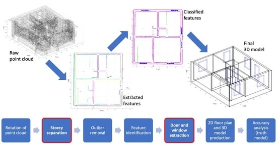
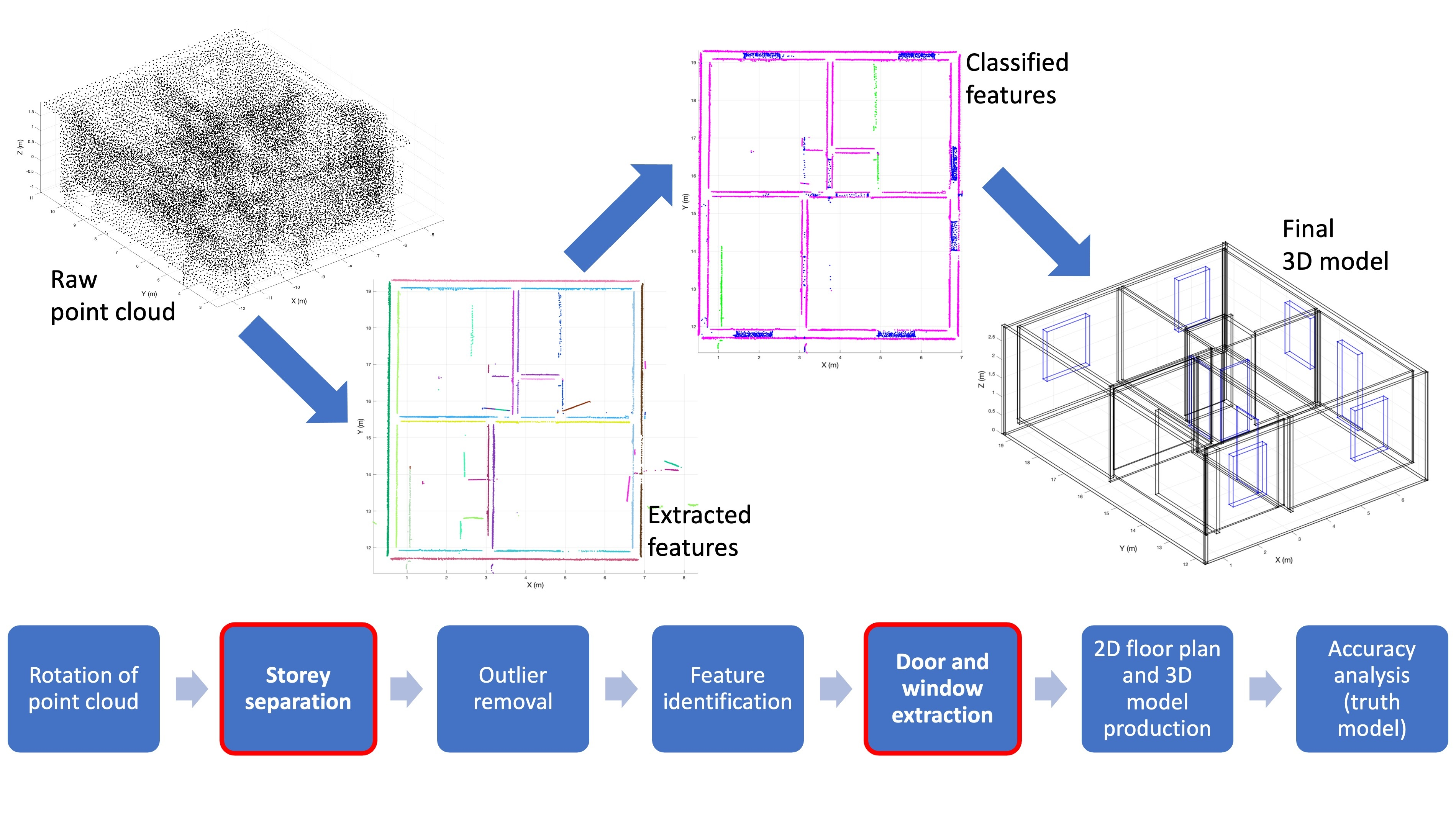
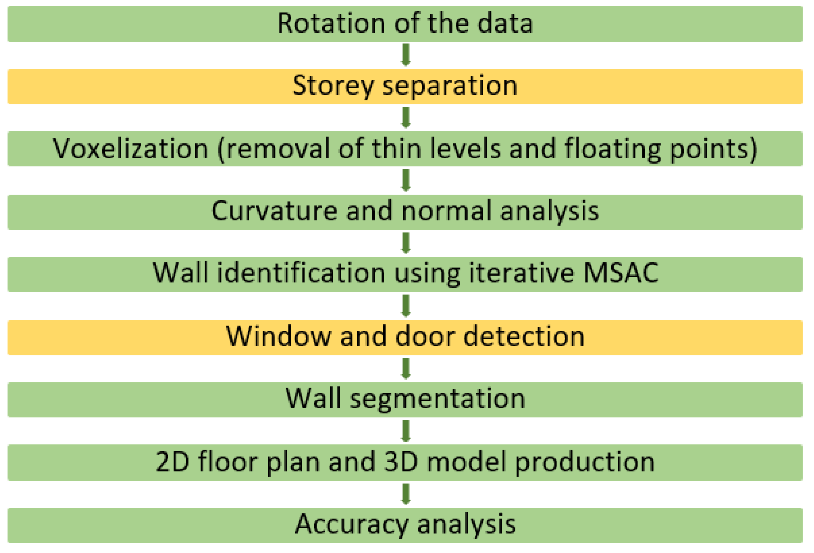
3. Methodology
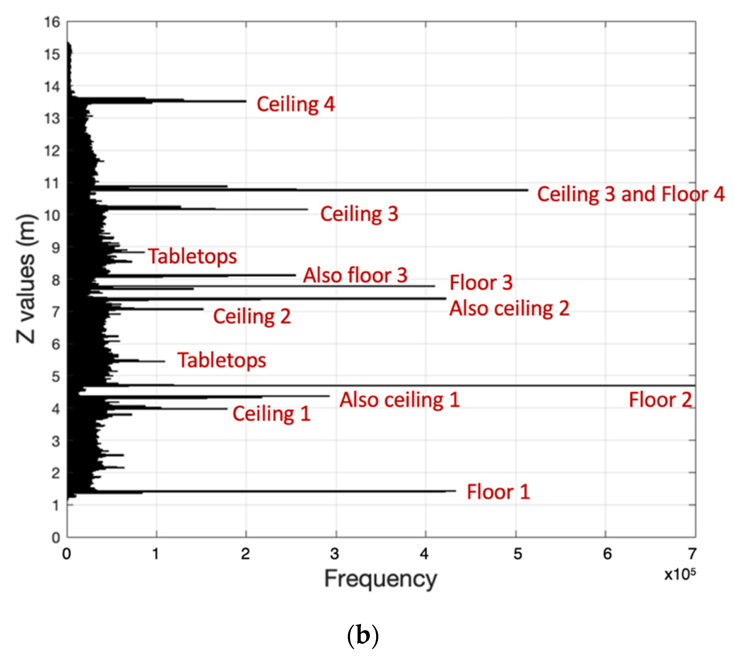
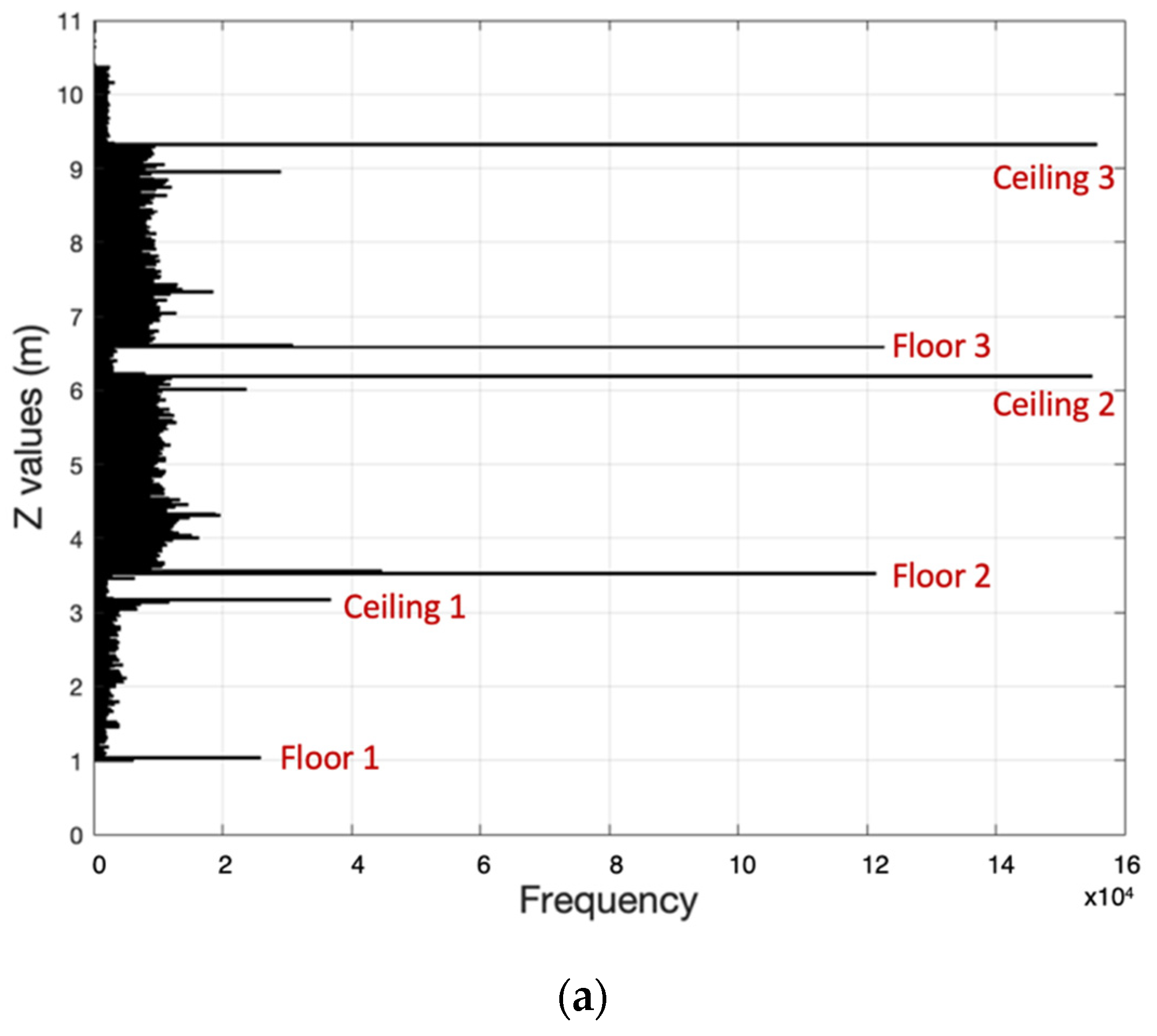
3.1. Storey Separation
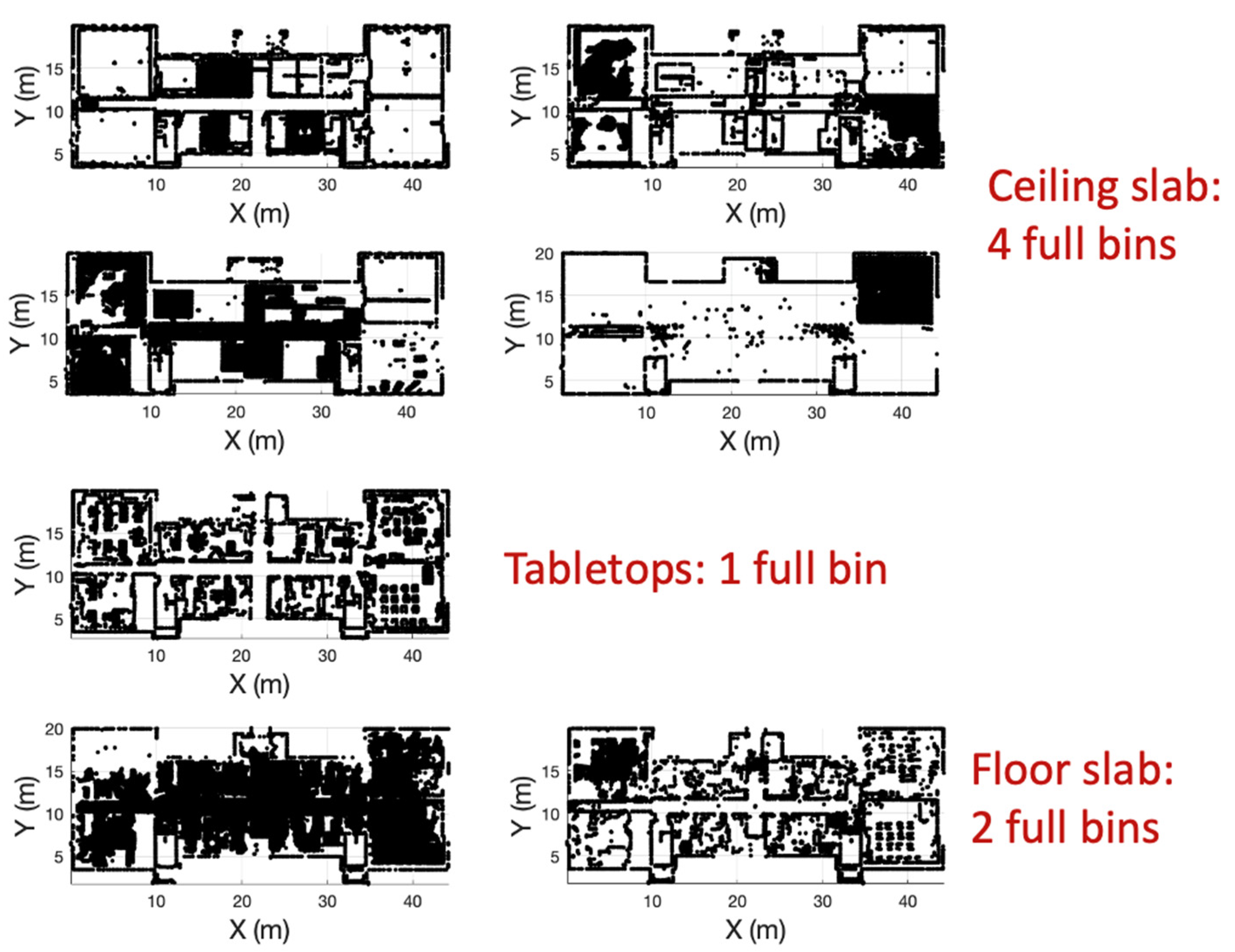
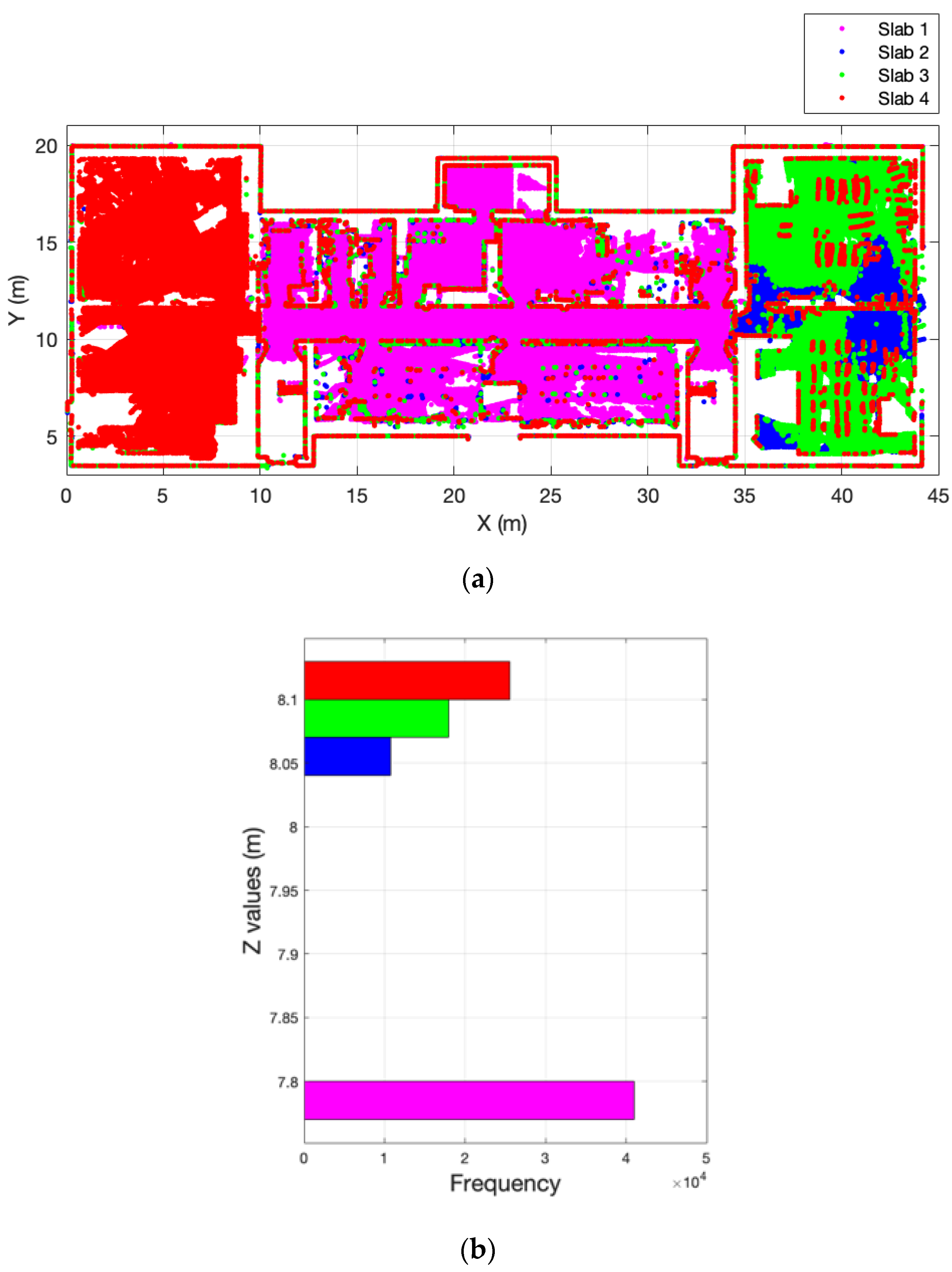
3.2. Data Cleaning and Feature Isolation
3.3. Wall Detection
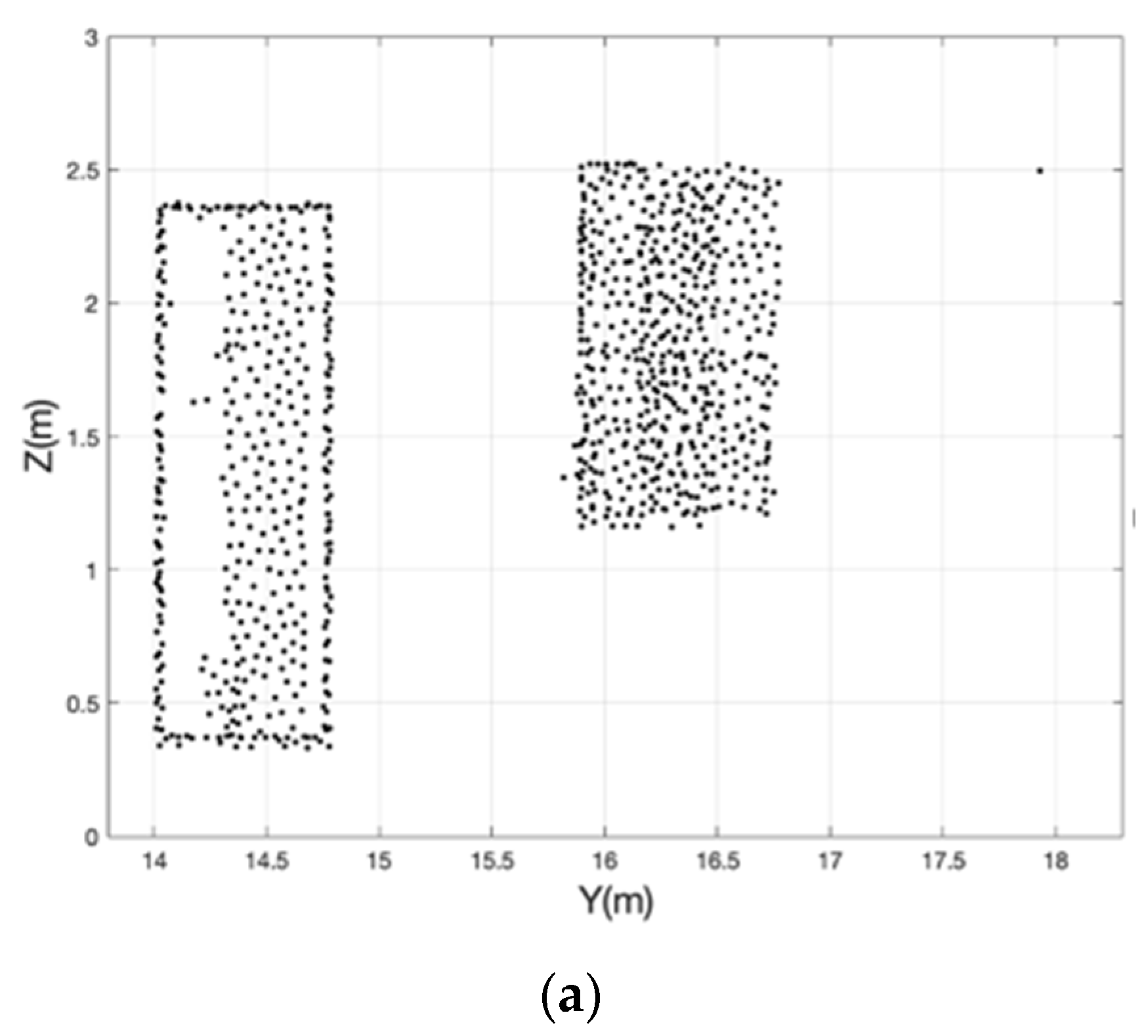
3.4. Door and Window Extraction
3.5. Quality Assessment
4. Dataset Description
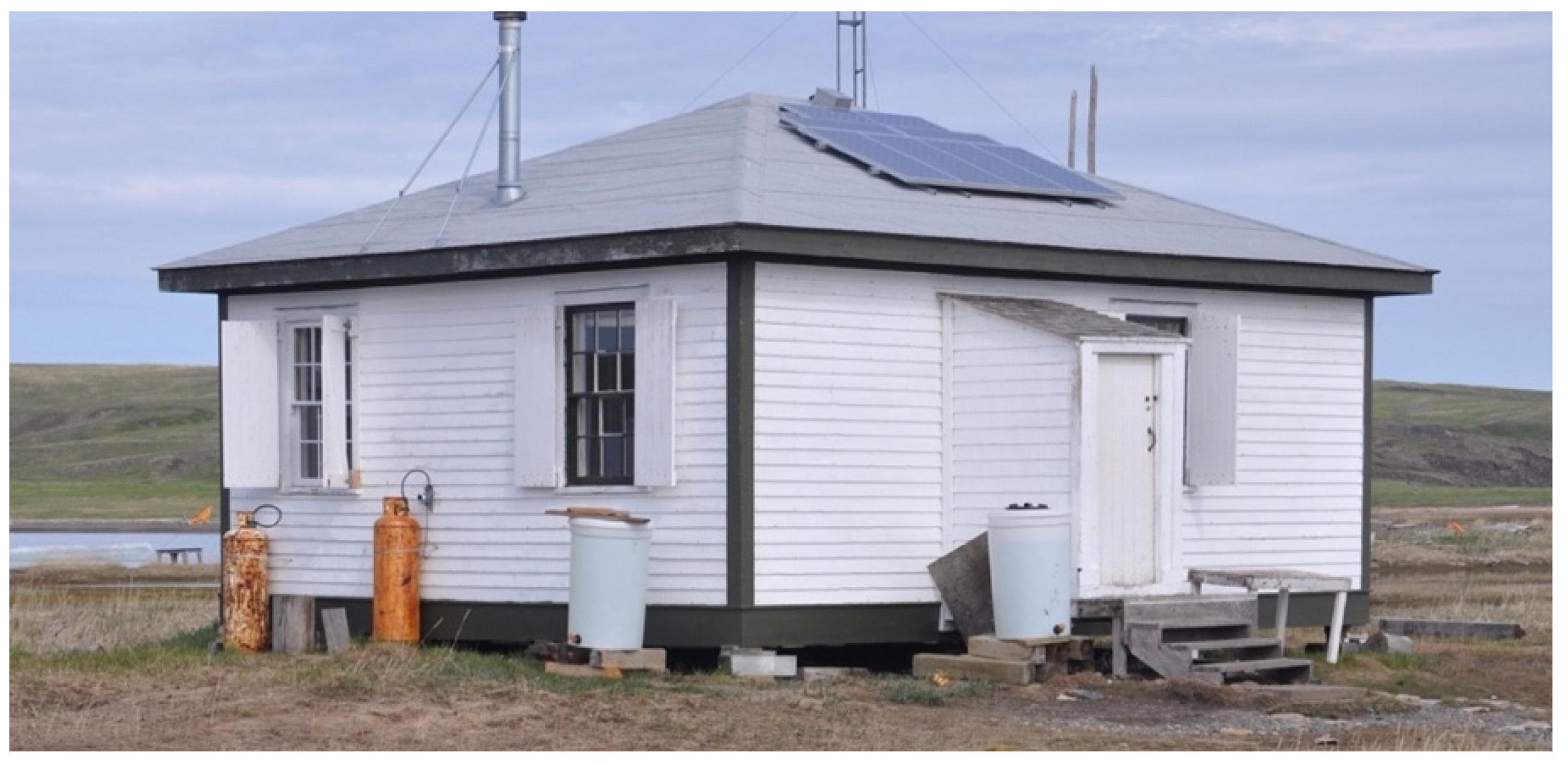
4.1. Signal House, Qikiqtaruk/Herschel Island, Territorial Park
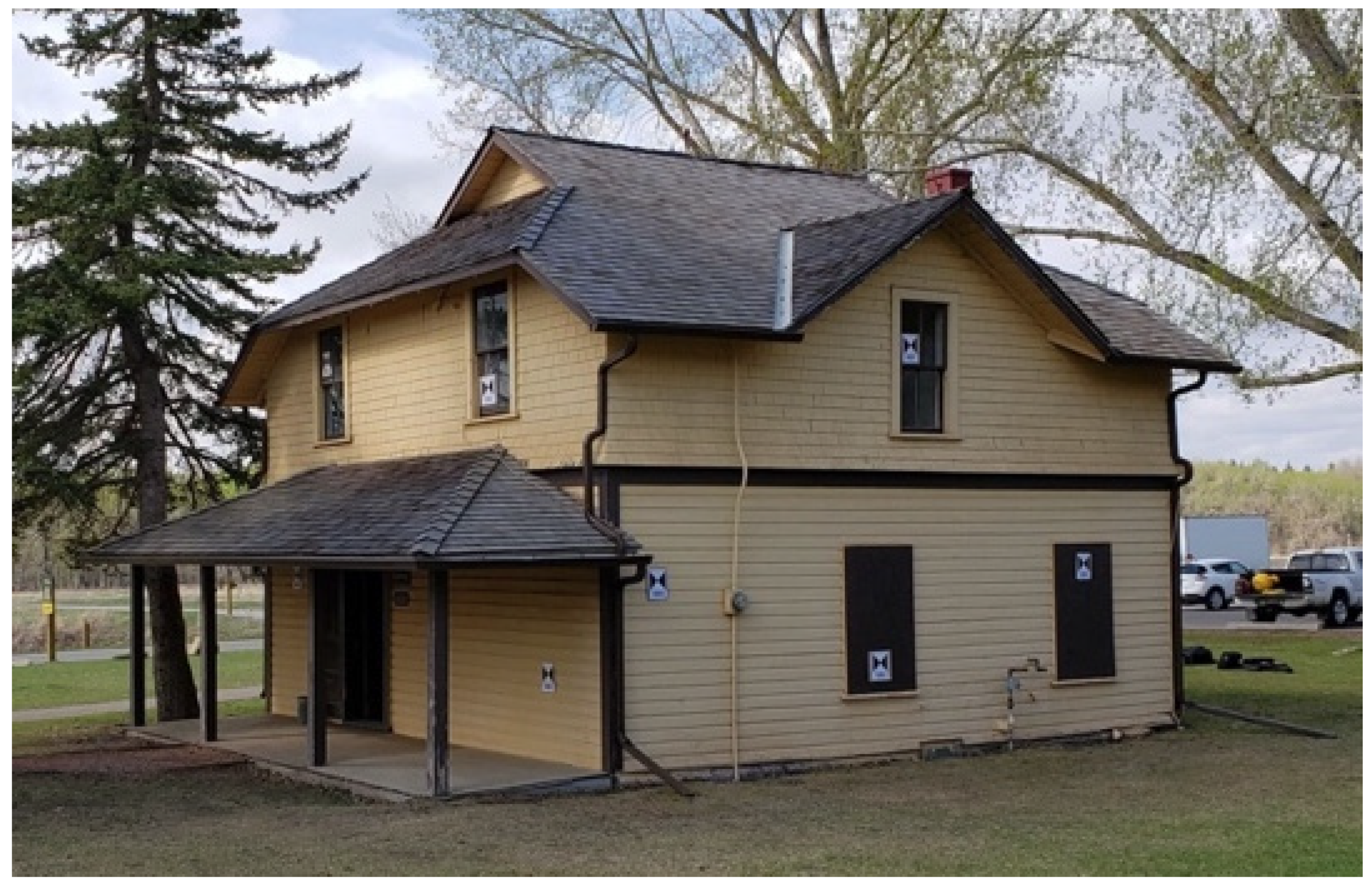
4.2. Jobber’s House, Fish Creek Provincial Park
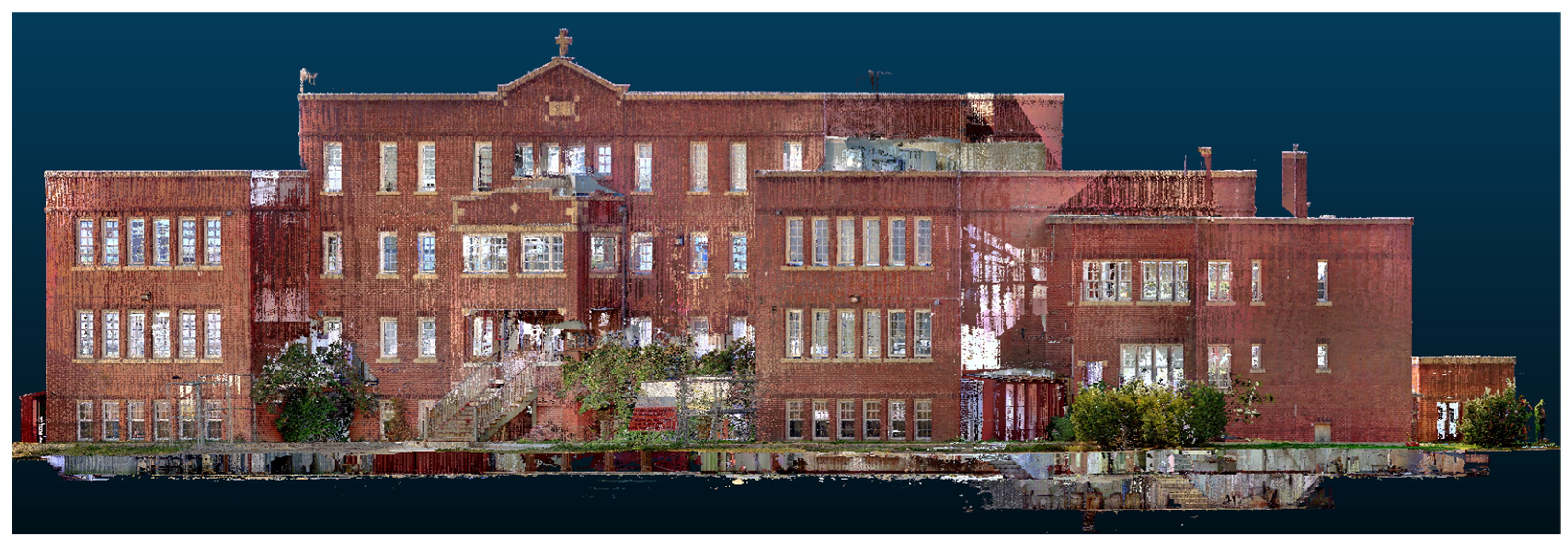
4.3. Old Sun Residential School
5. Results and Discussion
5.1. Storey Separation
5.2. Door and Window Extraction
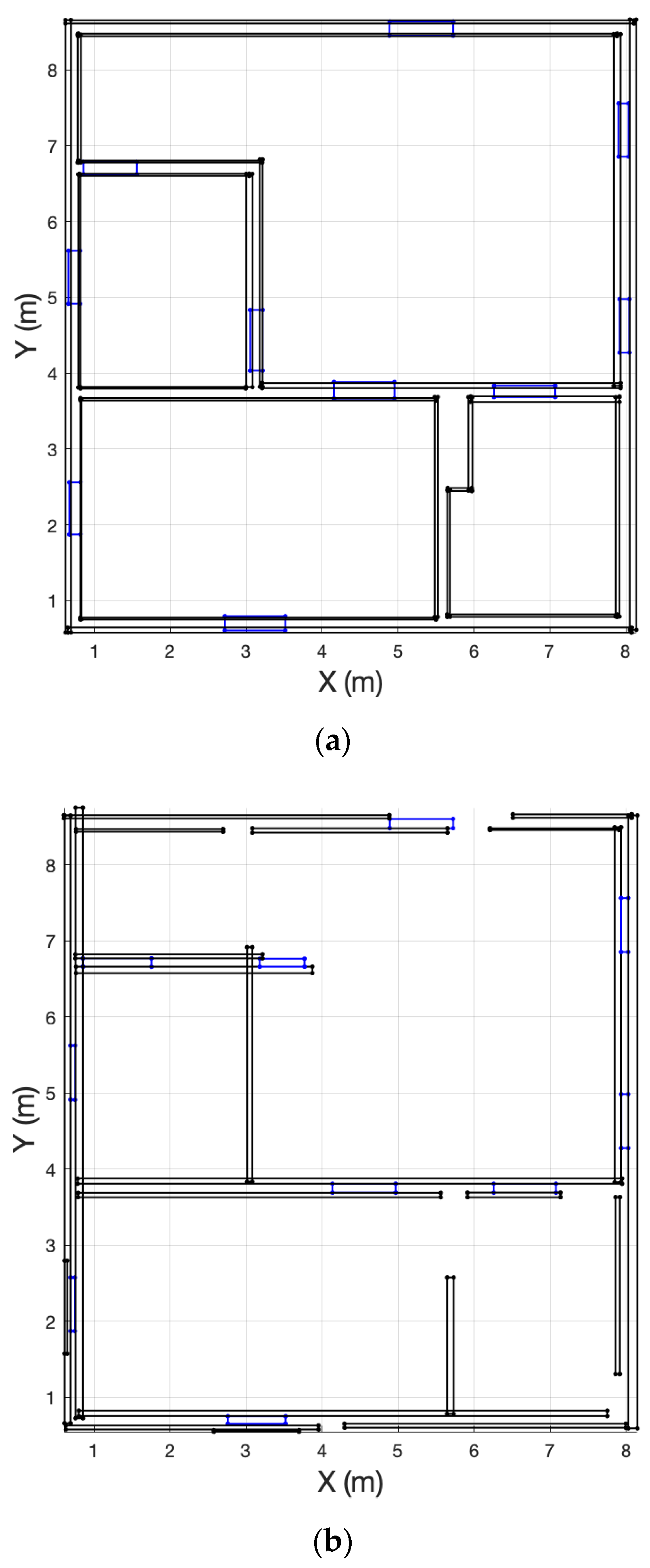
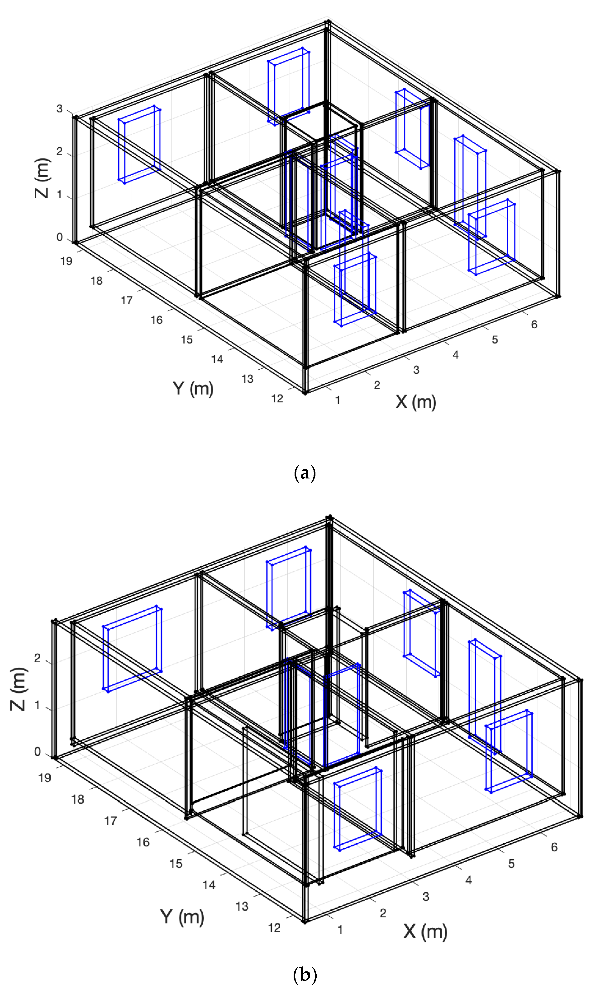
5.3. 2D Floor Plan and 3D Building Model Creation
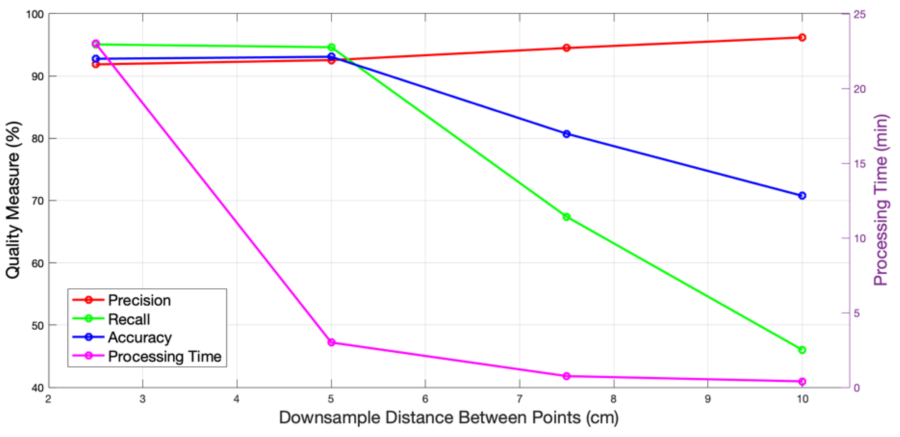
5.4. Down Sampling
6. Conclusions
Author Contributions
Funding
Institutional Review Board Statement
Informed Consent Statement
Data Availability Statement
Conflicts of Interest
References
- Thomson, C.; Boehm, J. Automatic Geometry Generation from Point Clouds for BIM. Remote Sens. 2015, 7, 11753–11775. [Google Scholar] [CrossRef] [Green Version]
- Khoshelham, K.; Díaz Vilariño, L. 3D Modelling of Interior Spaces: Learning the Language of Indoor Architecture. In Proceedings of the ISPRS Technical Commission V Symposium, Riva del Garda, Italy, 23–25 June 2014; Volume XL-5. [Google Scholar]
- Tran, H.; Khoshelham, K. Procedural Reconstruction of 3D Indoor Models from Lidar Data Using Reversible Jump Markov Chain Monte Carlo. Remote Sens. 2020, 12, 838. [Google Scholar] [CrossRef] [Green Version]
- Xia, S.; Chen, D.; Wang, R.; Li, J.; Zhang, X. Geometric Primitives in LiDAR Point Clouds: A Review. IEEE J. Sel. Top. Appl. Earth Obs. Remote Sens. 2020, 13, 685–707. [Google Scholar] [CrossRef]
- Xiao, J.; Furukawa, Y. Reconstructing the World’s Museums. In Proceedings of the Computer Vision—ECCV 2012, Florence, Italy, 7–13 October 2012; Fitzgibbon, A., Lazebnik, S., Perona, P., Sato, Y., Schmid, C., Eds.; Springer: Berlin/Heidelberg, Germany, 2012; pp. 668–681. [Google Scholar]
- Oesau, S.; Lafarge, F.; Alliez, P. Indoor scene reconstruction using feature sensitive primitive extraction and graph-cut. ISPRS J. Photogramm. Remote Sens. 2014, 90, 68–82. [Google Scholar] [CrossRef] [Green Version]
- Nurunnabi, A.; Belton, D.; West, G. Robust Segmentation for Large Volumes of Laser Scanning Three-Dimensional Point Cloud Data. IEEE Trans. Geosci. Remote Sens. 2016, 54, 4790–4805. [Google Scholar] [CrossRef]
- Yang, F.; Zhou, G.; Su, F.; Zuo, X.; Tang, L.; Liang, Y.; Zhu, H.; Li, L. Automatic Indoor Reconstruction from Point Clouds in Multi-room Environments with Curved Walls. Sensors 2019, 19, 3798. [Google Scholar] [CrossRef] [Green Version]
- Belton, D.; Mooney, B.; Snow, T.; Bae, K.-H. Automated Matching of Segmented Point Clouds to As-built Plans. In Proceedings of the Surveying and Spatial Sciences Conference 2011, Wellington, New Zealand, 21–25 November 2011. [Google Scholar]
- Xie, L.; Wang, R.; Ming, Z.; Chen, D. A Layer-Wise Strategy for Indoor As-Built Modeling Using Point Clouds. Appl. Sci. 2019, 9, 2904. [Google Scholar] [CrossRef] [Green Version]
- Bassier, M.; Vergauwen, M.; Van Genechten, B. Automated Classification of Heritage Buildings for As-Built BIM Using Machine Learning Techniques. ISPRS Ann. Photogramm. Remote Sens. Spat. Inf. Sci. 2017, IV-2/W2, 25–30. [Google Scholar] [CrossRef] [Green Version]
- Nguyen, A.; Le, B. 3D point cloud segmentation: A survey. In Proceedings of the 2013 6th IEEE Conference on Robotics, Automation and Mechatronics (RAM), Manila, Philippines, 12–15 November 2013; pp. 225–230. [Google Scholar]
- Grilli, E.; Menna, F.; Remondino, F. A Review of Point Clouds Segmentation and Classification Algorithms. In Proceedings of the ISPRS—International Archives of the Photogrammetry, Remote Sensing and Spatial Information Sciences, Nafplio, Greece, 1–3 March 2017; pp. 339–344. [Google Scholar]
- Turner, E.; Zakhor, A. Watertight As-Built Architectural Floor Plans Generated from Laser Range Data. In Proceedings of the Visualization Transmission 2012 Second International Conference on 3D Imaging, Modeling, Processing, Zurich, Switzerland, 13–15 October 2012; pp. 316–323. [Google Scholar]
- Li, L.; Su, F.; Yang, F.; Zhu, H.; Li, D.; Zuo, X.; Li, F.; Liu, Y.; Ying, S. Reconstruction of Three-Dimensional (3D) Indoor Interiors with Multiple Stories via Comprehensive Segmentation. Remote Sens. 2018, 10, 1281. [Google Scholar] [CrossRef] [Green Version]
- Macher, H.; Landes, T.; Grussenmeyer, P. From Point Clouds to Building Information Models: 3D Semi-Automatic Reconstruction of Indoors of Existing Buildings. Appl. Sci. 2017, 7, 1030. [Google Scholar] [CrossRef] [Green Version]
- Babacan, K.; Jung, J.; Wichmann, A.; Jahromi, B.A.; Shahbazi, M.; Sohn, G.; Kada, M. Towards Object Driven Floor Plan Extraction from Laser Point Clouds. ISPRS Int. Arch. Photogramm. Remote Sens. Spat. Inf. Sci. 2016, XLI-B3, 3–10. [Google Scholar] [CrossRef] [Green Version]
- Xia, S.; Wang, R. Façade Separation in Ground-Based LiDAR Point Clouds Based on Edges and Windows. IEEE J. Sel. Top. Appl. Earth Obs. Remote Sens. 2019, 12, 1041–1052. [Google Scholar] [CrossRef]
- Jung, J.; Stachniss, C.; Ju, S.; Heo, J. Automated 3D volumetric reconstruction of multiple-room building interiors for as-built BIM. Adv. Eng. Inform. 2018, 38, 811–825. [Google Scholar] [CrossRef]
- Previtali, M.; Díaz-Vilariño, L.; Scaioni, M. Towards Automatic Reconstruction of Indoor Scenes from Incomplete Point Clouds: Door and Window Detection and Regularization. ISPRS Int. Arch. Photogramm. Remote Sens. Spat. Inf. Sci. 2018, XLII–4, 507–514. [Google Scholar] [CrossRef] [Green Version]
- Zheng, Y.; Peter, M.; Zhong, R.; Oude Elberink, S.; Zhou, Q. Space Subdivision in Indoor Mobile Laser Scanning Point Clouds Based on Scanline Analysis. Sensors 2018, 18, 1838. [Google Scholar] [CrossRef] [Green Version]
- Budroni, A.; Böhm, J. Automatics 3D modelling of indoor Manhattan-World scenes from laser data. Int. Arch. Photogramm. Remote Sens. Spat. Inf. Sci. 2010, 38, 115–120. [Google Scholar]
- Michailidis, G.-T.; Pajarola, R. Bayesian graph-cut optimization for wall surfaces reconstruction in indoor environments. Vis. Comput. 2017, 33, 1347–1355. [Google Scholar] [CrossRef] [Green Version]
- Zhang, R.; Zakhor, A. Automatic identification of window regions on indoor point clouds using LiDAR and cameras. In Proceedings of the IEEE Winter Conference on Applications of Computer Vision, Steamboat Springs, CO, USA, 24–26 March 2014; pp. 107–114. [Google Scholar]
- Díaz-Vilariño, L.; Khoshelham, K.; Martínez-Sánchez, J.; Arias, P. 3D Modeling of Building Indoor Spaces and Closed Doors from Imagery and Point Clouds. Sensors 2015, 15, 3491–3512. [Google Scholar] [CrossRef] [PubMed] [Green Version]
- Quintana, B.; Prieto, S.A.; Adán, A.; Bosché, F. Door detection in 3D coloured point clouds of indoor environments. Autom. Constr. 2018, 85, 146–166. [Google Scholar] [CrossRef]
- Leys, C.; Ley, C.; Klein, O.; Bernard, P.; Licata, L. Detecting outliers: Do not use standard deviation around the mean, use absolute deviation around the median. J. Exp. Soc. Psychol. 2013, 49, 764–766. [Google Scholar] [CrossRef] [Green Version]
- Fischler, M.; Bolles, R. Random Sample Consensus: A Paradigm for Model Fitting with Applications to Image Analysis and Automated Cartography. Available online: http://www.cs.ait.ac.th/~mdailey/cvreadings/Fischler-RANSAC.pdf (accessed on 28 April 2020).
- Torr, P.H.S.; Zisserman, A. MLESAC: A New Robust Estimator with Application to Estimating Image Geometry. Comput. Vis. Image Underst. 2000, 78, 138–156. [Google Scholar] [CrossRef] [Green Version]
- Zuliani, M. RANSAC for Dummies 2008; Vision Research Lab, University of California: Santa Barbara, CA, USA, 2009. [Google Scholar]
- National Research Council Canada; Associate Committee on the National Building Code; Canadian Commission on Building and Fire Codes. National Building Code of Canada; Associate Committee on the National Building Code, National Research Council of Canada: Ottawa, ON, Canada, 2010; ISBN 978-0-660-19975-7.
- Okorn, B.; Pl, V.; Xiong, X.; Akinci, B.; Huber, D. Toward Automated Modeling of Floor Plans. In Proceedings of the Symposium on 3D Data Processing, Visualization and Transmission, Espace Saint Martin, Paris, France, 17–20 May 2010. [Google Scholar]
- Oesau, S.; Lafarge, F.; Alliez, P. Indoor Scene Reconstruction using Primitive-driven Space Partitioning and Graph-cut. Eurographics Workshop Urban Data Model. Vis. 2013. [Google Scholar] [CrossRef]
- Maalek, R.; Lichti, D.D.; Ruwanpura, J.Y. Robust Segmentation of Planar and Linear Features of Terrestrial Laser Scanner Point Clouds Acquired from Construction Sites. Sensors 2018, 18, 819. [Google Scholar] [CrossRef] [PubMed]


| Dataset | Sample Size (# Points) | Precision | Recall | Accuracy |
|---|---|---|---|---|
| Jobber’s House Storey 2 | 16,491 | 87.93% | 57.94% | 94.27% |
| Old Sun Rear Building Storey 2 | 54,593 | 93.42% | 90.94% | 96.30% |
| Old Sun Main Building Storey 3 | 212,517 | 85.65% | 95.80% | 93.65% |
| Dataset | Doors | Windows | False Detections | ||
|---|---|---|---|---|---|
| Truth Model | Calculated Model | Truth Model | Calculated Model | ||
| Signal House | 5 | 5 | 5 | 5 | 0 |
| Jobber’s House Storey 1 | 6 | 5 | 4 | 4 | 1 |
| Old Sun Annex Storey 3 | 5 | 3 | 9 | 8 | 1 |
| Old Sun Main Building Storey 3 | 16 | 2 | 48 | 35 | 8 |
| Feature | Width Difference (m) | Height Difference (m) |
|---|---|---|
| Window 1 | 0.131 | −0.036 |
| Window 2 | 0.342 | −0.069 |
| Window 3 | 0.030 | −0.013 |
| Window 4 | 0.093 | 0.056 |
| Window 5 | −0.034 | 0.056 |
| Door 1 | 0.023 | 0.044 |
| Door 2 | 0.024 | −0.045 |
| Door 3 | 0.016 | 0.018 |
| Door 4 | 0.029 | −0.066 |
| Absolute mean difference: | 0.080 | 0.045 |
| Dataset | Sample Size (# Points) | Precision | Recall | Accuracy |
|---|---|---|---|---|
| Signal House | 82,607 | 96.70% | 96.20% | 96.14% |
| Jobber’s House Storey 1 | 106,229 | 92.47% | 92.86% | 94.05% |
| Old Sun Annex Storey 3 | 118,052 | 92.67% | 92.94% | 92.72% |
| Old Sun Main Building Storey 3 | 605,761 | 82.64% | 86.86% | 88.10% |
Publisher’s Note: MDPI stays neutral with regard to jurisdictional claims in published maps and institutional affiliations. |
© 2021 by the authors. Licensee MDPI, Basel, Switzerland. This article is an open access article distributed under the terms and conditions of the Creative Commons Attribution (CC BY) license (https://creativecommons.org/licenses/by/4.0/).
Share and Cite
Pexman, K.; Lichti, D.D.; Dawson, P. Automated Storey Separation and Door and Window Extraction for Building Models from Complete Laser Scans. Remote Sens. 2021, 13, 3384. https://doi.org/10.3390/rs13173384
Pexman K, Lichti DD, Dawson P. Automated Storey Separation and Door and Window Extraction for Building Models from Complete Laser Scans. Remote Sensing. 2021; 13(17):3384. https://doi.org/10.3390/rs13173384
Chicago/Turabian StylePexman, Kate, Derek D. Lichti, and Peter Dawson. 2021. "Automated Storey Separation and Door and Window Extraction for Building Models from Complete Laser Scans" Remote Sensing 13, no. 17: 3384. https://doi.org/10.3390/rs13173384
APA StylePexman, K., Lichti, D. D., & Dawson, P. (2021). Automated Storey Separation and Door and Window Extraction for Building Models from Complete Laser Scans. Remote Sensing, 13(17), 3384. https://doi.org/10.3390/rs13173384