Article

Landslide Detection from Open Satellite Imagery Using Distant Domain Transfer Learning

College of Construction Engineering, Jilin University, Changchun 130026, China
*
Author to whom correspondence should be addressed.
Remote Sens. 2021, 13(17), 3383; https://doi.org/10.3390/rs13173383
Submission received: 22 June 2021 / Revised: 8 August 2021 / Accepted: 26 August 2021 / Published: 26 August 2021

Abstract

:
Using convolutional neural network (CNN) methods and satellite images for landslide identification and classification is a very efficient and popular task in geological hazard investigations. However, traditional CNNs have two disadvantages: (1) insufficient training images from the study area and (2) uneven distribution of the training set and validation set. In this paper, we introduced distant domain transfer learning (DDTL) methods for landslide detection and classification. We first introduce scene classification satellite imagery into the landslide detection task. In addition, in order to more effectively extract information from satellite images, we innovatively add an attention mechanism to DDTL (AM-DDTL). In this paper, the Longgang study area, a district in Shenzhen City, Guangdong Province, has only 177 samples as the landslide target domain. We examine the effect of DDTL by comparing three methods: the convolutional CNN, pretrained model and DDTL. We compare different attention mechanisms based on the DDTL. The experimental results show that the DDTL method has better detection performance than the normal CNN, and the AM-DDTL models achieve 94% classification accuracy, which is 7% higher than the conventional DDTL method. The requirements for the detection and classification of potential landslides at different disaster zones can be met by applying the AM-DDTL algorithm, which outperforms traditional CNN methods.

1. Introduction

With the rapid development of cities, urban construction sites have expanded to low hills, with engineering construction occurring on many unstable slopes [1]. Under extreme cases, such as seismic shaking and heavy rainfall, these unstable slopes can easily become landslides and cause severe damage to the natural environment, property and personal safety [2,3]. For example, on 7 June 2008, heavy rainfall triggered many landslides, debris flows and floods in the Hong Kong area [4]. As landslides often cause serious destruction to human settlements, roads and agricultural lands, we must identify and manage potential landslide areas and warn citizens about their occurrence in order: to ensure their safety [5]. Currently, two methods are used to identify potential landslides: field investigation and indoor remote sensing interpretation [6]. Although the first method is effective and accurate for landslide detection, it requires considerable labor, material and financial resources [7]. For remote sensing interpretation, specialists judge whether a landslide has occurred according to optical images, digital elevation model (DEM) data and other geological information [8]. This method is time-consuming and its interpretation accuracy may be poor [8,9]. Therefore, a novel method that can automatically recognize landslides must be constructed based on new technologies and new methods [10].
New technologies, such as machine learning, have produced unprecedented opportunities for the prediction, identification and management of geological disasters in the era of big data [11]. Landslide detection is regarded as the study of satellite image recognition and classification [6]. Machine learning methods, such as support vector machines (SVMs) [12,13], artificial neural networks (ANNs) [14] and deep learning, have been extensively used in landslide research [1,15], especially convolutional neural networks (CNNs), which have become a research focus in the field of landslide detection [16,17]. The SVM, ANN, RF and CNN methods have been used for potential landslide detection using optical remote sensing images and topography [18], and the CNN has been considerably improved as the mainstream deep learning method used to extract information from remote sensing images [19]. A residual network based on the CNN was designed for landslide detection [20]. To detect special slope failures, the CNN approach was developed [21]. For images with diverse spectral characteristics, a recognition method based on CNNs was proposed [21]. Fully convolutional networks (FCNs) and patch-based deep convolutional neural networks (DCNNs) were used to classify land cover types [22]. A CNN with a suitable input image size and training strategies is effective for slope failure detection [23]. The new method combining CNN and multilayer has been applied to the classification of very-high-resolution remote sensing imagery and displayed better performance [24]. For land cover classification tasks, the attentive spatial temporal graph CNN can exploit both spatial and temporal dimensions in satellite images and time series data [25]. The attention mechanisms have been gradually introduced into the structure of CNN. They include channel attention, spatial attention and non-local attention; these three kinds of attention mechanisms perform better on super-resolution single images [26]. Moreover, a deep neural network equipped with a control gate and feedback attention mechanism can perform pixel-wise classification for very-high-resolution remote sensing images [27]. Combining a CNN and attention mechanism can lead to good performance for landslide detection [6].
Machine learning has two requirements before training a classification model: it needs sufficient training data, and the training data must have the same distribution as the validation data [28,29]. Unfortunately, in this study, the study area, Longgang, China, is unique and has only 177 landslide samples, which is not enough to train a robust classification model. Obtaining labeled training data always requires considerable costs and has limitations [1,28]. Therefore, we introduce the transfer learning algorithm to solve the problem [29,30]. Transfer learning can eliminate these two disadvantages by transferring knowledge from the source domain to the target domain [31].
Transfer learning assumes that the source domain and the target domain are more or less similar [32,33], but for the landslide detection problem, few open landslide datasets are available as the source domain [6,28]. Therefore, we first introduce distant domain transfer learning (DDTL) for remote sensing imagery classification. The DDTL algorithm only needs a small amount of labeled target data and unlabeled source data from completely different domains [34]. In addition, we first apply the scene classification dataset to the landslide classification task as the source domain. Then, we creatively integrate the attention module into the DDTL framework because the attention mechanism can extract the key information and suppress redundant, useless information, thus improving the results of the model [35,36].

2. Materials

2.1. Study Area and Dataset

The study covers the whole Longgang district in the city of Shenzhen, Guangdong Province, China, with an area of 388.22 km2, as shown in Figure 1. The topography of Longgang District is complex and dominated by low mountains and hills. The central part of this region is a low-lying alluvial plain, which easily catches water. In the subtropical ocean monsoon zone, the average annual rainfall of this region is 1935.8 mm, and landslides often occur, resulting from heavy rainfall due to strong typhoons [16,37].
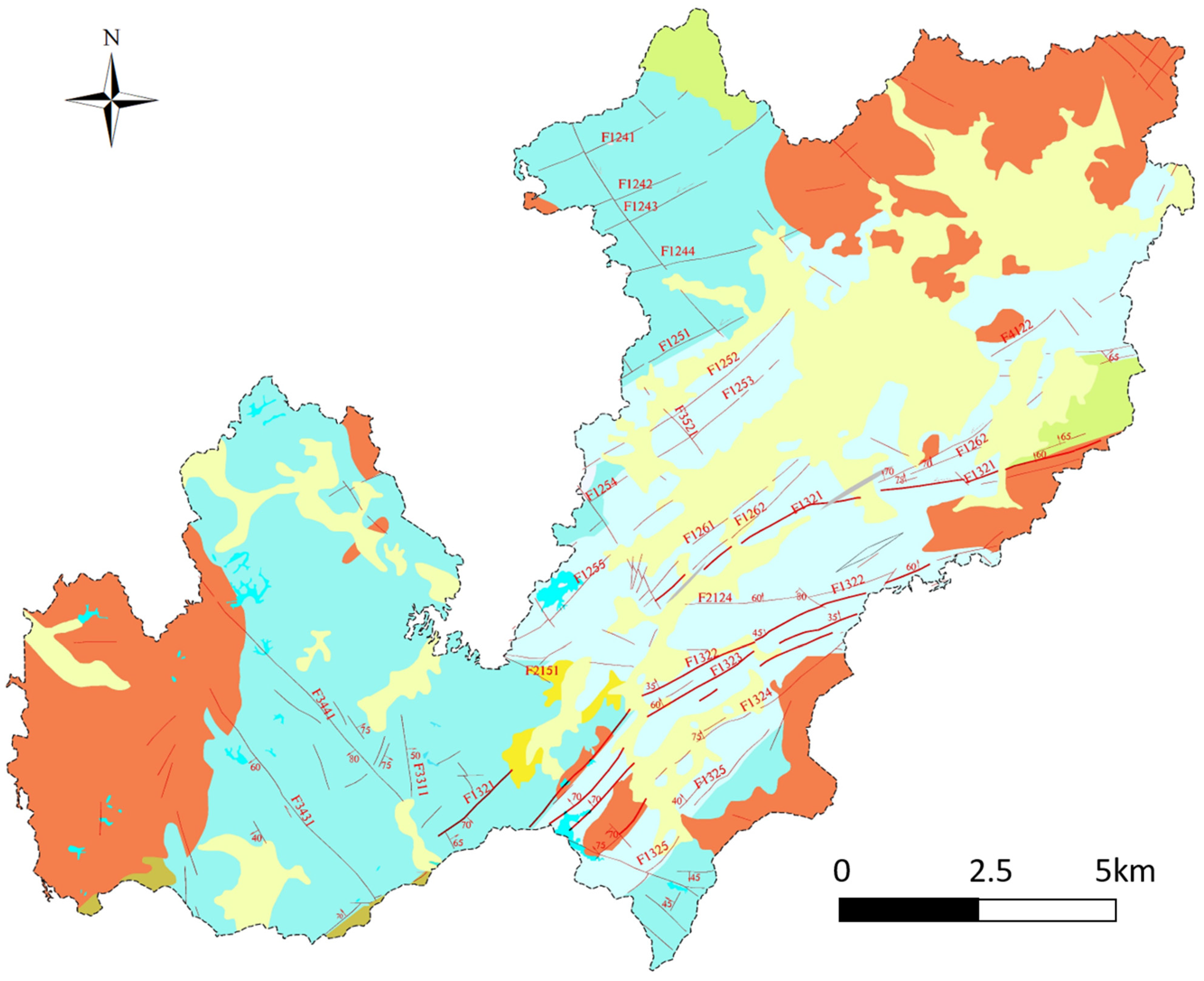
The stability of the slopes in this study area is poor because the thick, weathered soil layer has low strength within the range of influence of the fault zone [38]. The fault zone of Longgang District is shown in Figure 2. Urban construction sites have expanded to low hills and platform areas, the original shape of the hillsides has changed, and the stability of the mountains has been degraded by intense human engineering activities. Under severe conditions, such as concentrated rainfall or earthquakes, the reduction in the mechanical strength of the soil can easily cause landslides and other geological disasters [12,39]. For example, on 20 December 2015, a landslide on an unstable artificial slope composed of construction waste destroyed almost all the buildings along the flow path [40,41].
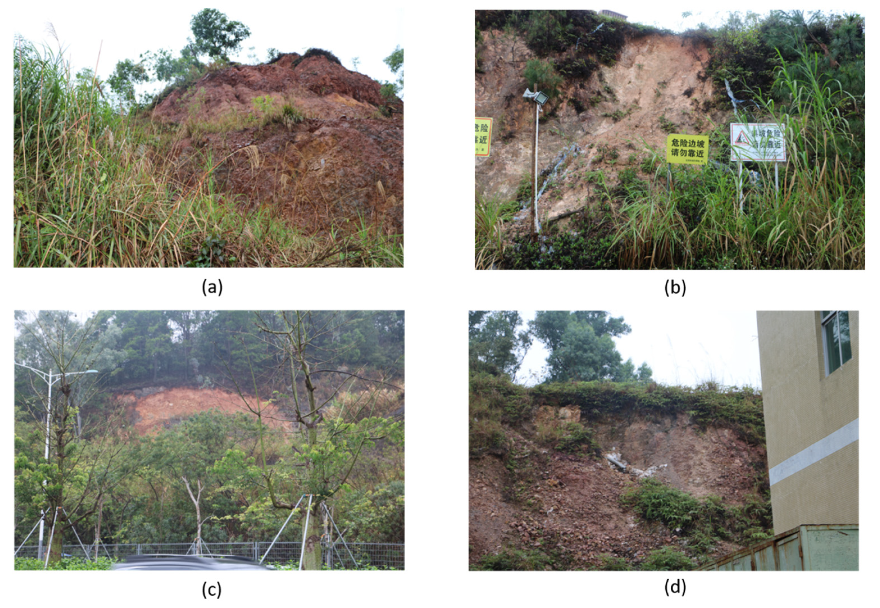
Due to the natural environment and engineering activities, many landslides result from unstable slopes in this region [1], as shown in Figure 3. In the dataset used in this study, 177 landslides, including collapses, a few mudslides and mainly unstable slopes, were interpreted by experts with satellite images and other geological information. Subsequently, we selected 431 non-landslide regions, including supported stable slopes and some roads, rivers, farmland and residential areas. Compared to other landslide datasets, the Longgang landslide dataset is more complicated and unique because it contains many supported stable slopes, which are difficult for computer vision to recognize. The landslides in this region are mainly caused by artificially unstable slopes with a certain space geometry and certain texture features [42]. In addition, satellite images contain much useless information because roads and houses are situated near unstable slopes in low hill areas.

2.2. The Source Domain Datasets

In this section, we introduce the source domains used in the distant domain transfer learning algorithm as shown in the Table 1. The primary source domain is the Bijie landslide dataset [6]. The auxiliary source domains are the UC Merced land use dataset [31,43], the Google image datasets of SIRI-WHU and WHU-RS19 [43,44,45] and the NWPU-RESISC45 dataset [46].
The Bijie landslide dataset, for the city of Bijie, Guizhou Province, consists of 770 landslide samples and 2003 negative samples. The dataset is visually similar to the Longgang target domain. The landslide images mainly include rock falls and rock slides, while the environmental remote sensing images consisting of mountains, villages, roads, rivers, forests and agricultural land were chosen manually [6]. To the best of our knowledge, this dataset is the only open, accurate and large remote sensing landslide dataset. Landslides were created to promote automatic landslide detection studies using optical remote sensing images, although the features of landslides differ between regions.
The UC Merced land use dataset has 21 classes of land use image datasets meant for research purposes, and each class has 100 images. The images were manually extracted from large images from the USGS National Map Urban Area Imagery collection for various urban areas around the country. The pixel resolution of this public domain imagery is 1 foot. Each image measures 256 × 256 pixels [31,43].
The SIRI-WHU dataset contains 200 images for 12 classes, and each image measures 200 × 200 pixels, with a 2 m spatial resolution. This dataset was acquired from Google Earth (Google Inc.) and mainly covers urban areas in China, and the scene image dataset was designed by the RS_IDEA Group in Wuhan University (SIRI-WHU) [43,44,45].
The WHU-RS19 dataset contains 12 categories of physical scenes in satellite imagery collected from Google Earth. The dataset consists of airports, bridges, rivers, forests, meadows, ponds, parking, ports, viaducts, residential areas, industrial areas and commercial areas, with 50 samples for each class. This dataset has a total of 1005 images [47].
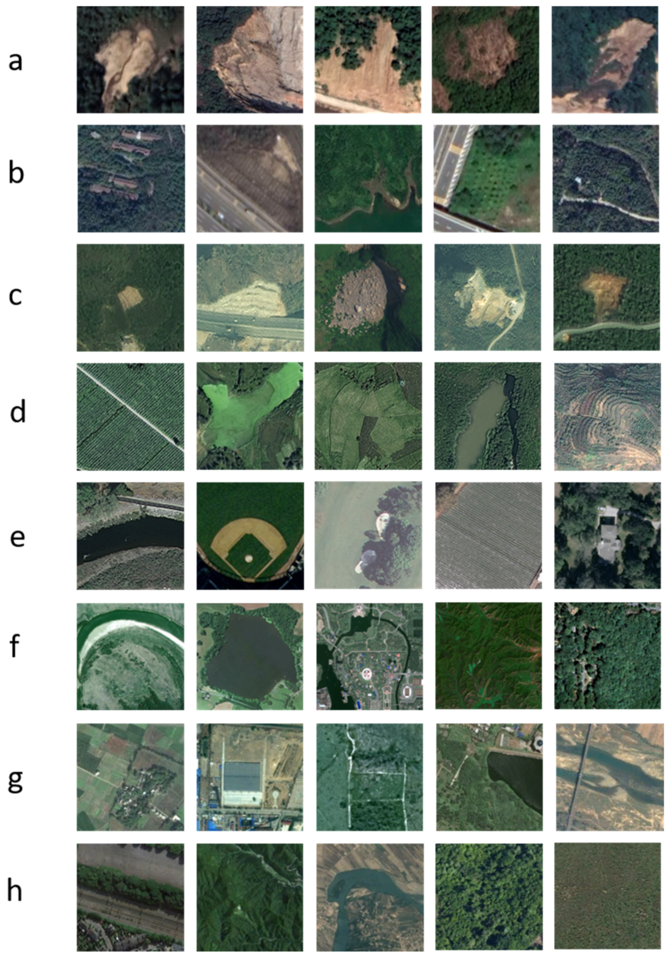
The NWPU-RESISC45 dataset, consisting of 31,500 images, has 45 scene classes with 700 images in each class, created by Northwestern Polytechnical University (NWPU) for remote sensing image classification. Similar to other remote sensing datasets, the 45 classes of this dataset include the same scene images, such as airplanes, airports and beaches [46]. The remote sensing images of the Longgang landslide dataset and the five source domain datasets are shown in Figure 4.

3. Methods

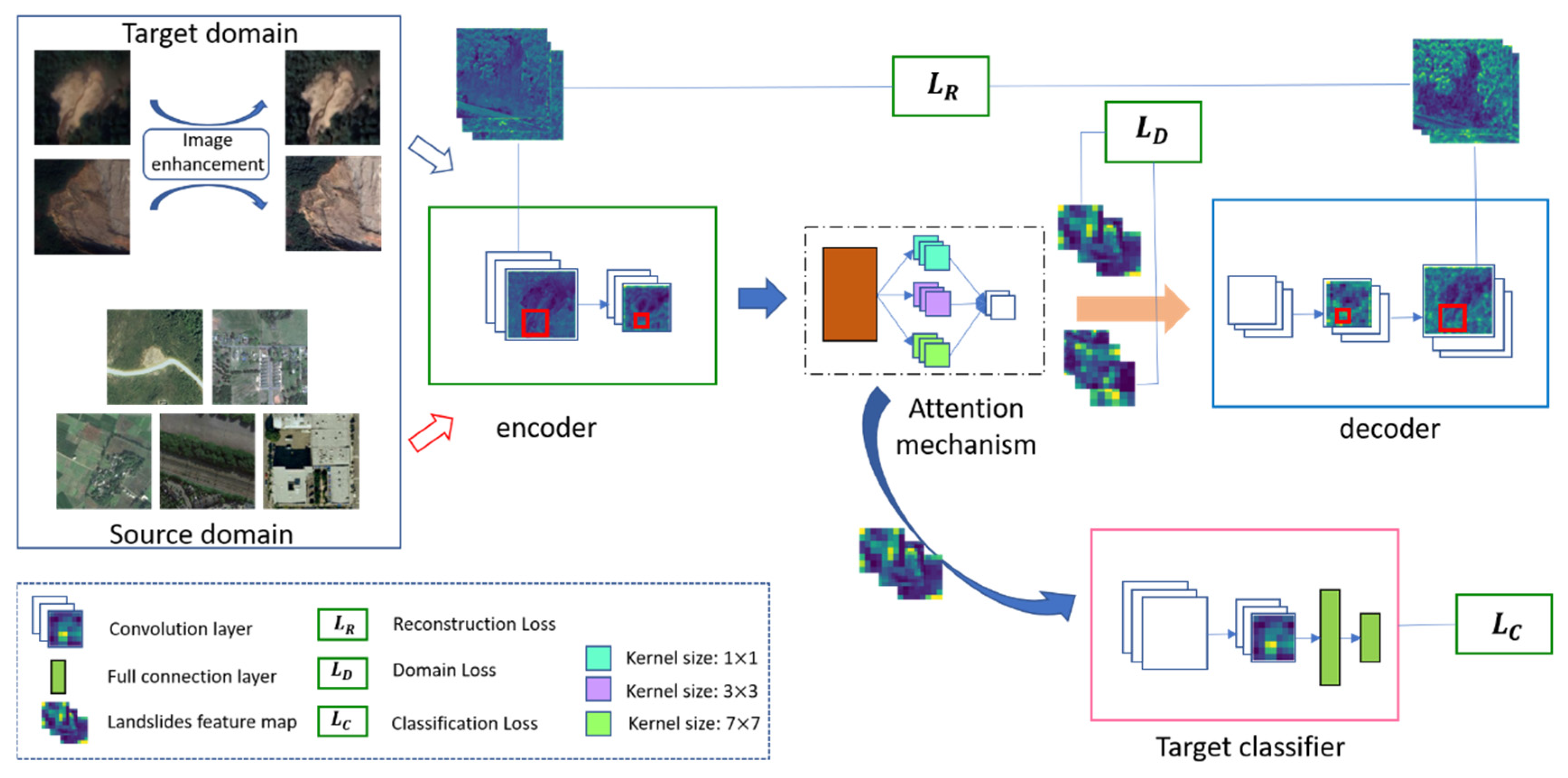
In this study, we applied the distant domain transfer learning algorithm for Longgang landslide detection. Moreover, we combined the DDTL and the attention module to refine the feature maps and improve the performance of target classification. In this section, we first introduce the image enhancement approach; then, we briefly review the theory of distant domain transfer learning and attention modules, and we subsequently introduce the improved attention module. For comparison, we also introduce the traditional CNN model and the similar pretrained transfer learning model.

3.1. Image Enhancement

Optical remote sensing images are carriers of natural information, and only interpreting the natural information of these images can realize their application value. However, for some blurry and shadowed remote sensing images, it is necessary to enhance their quality. The technology of image enhancement, using a series of algorithms, enhances the useful information and improves the visual quality in order to meet the requirements of computer vision [48].
Improving the quality of images using image enhancement techniques is crucial for preparing image datasets. To apply deep learning methods for image classification, it is necessary to improve the remote sensing image quality in order to obtain good training outcomes. Low-illumination optical remote sensing images, because of uneven light or other reasons, have poor visual effects, and the differences in the image features are low, so they cannot meet the requirements of image classification and recognition [49].
Among the Longgang landslide images are many low-light images from Google Earth, so, in this paper, we introduce the image contrast enhancement algorithm to process the images in order to improve the remote sensing image quality for computer vision systems [50].
To solve the enhancement problem, the contrast enhancement algorithm fuses the input image P with the processed image under another exposure to reduce the complexity [50]. The overall formula for calculating the fused image is defined as follows:
R c = W P c + ( 1 W ) g ( P c , k )
where W is the weight matrix, which can enhance the low contrast of underexposed regions and preserve the well-exposed regions; c is the index of three color channels; R is the enhanced result. The weight matrix is calculated as follows:
W = T μ .  
where T is the scene illumination map solved by optimization, and μ is a parameter controlling the enhancement degree. More details about the optimization problem are provided in [50].
In the algorithm, because no information about the picture is available, we use the fixed parameters (a = −0.3293, b = 1.1258) to calculate g ( P c , k ) [50,51]. The formula is as follows:
g ( P c , k ) = e b ( 1 k a ) P ( k a )
Finally, the parameter k is calculated by maximizing the image entropy of the enhancement brightness as follows.
k ^ = argmax k ( g ( B , k ) ) .
( B ) = i N p i · log 2 p i
To improve the calculation efficiency, we resize the input image to 50 × 50 when optimizing k, where B is the brightness component, p i is the beam of the histogram of B, and N is often set to 256.

3.2. Distant Domain Transfer Learning

Similar to traditional machine learning, transfer learning has gradually emerged as a focus of research and will become popular in the information field because of its unique advantages [52]. Regarding the scarcity of research landslide images, transfer learning can improve the model performance by transferring knowledge from source domain data [53]. For traditional transfer learning, the source domain and the target domain should be similar or have a certain connection [54]. In this way, the dependence on constructing the target model with much labeled target data can be reduced [55,56].
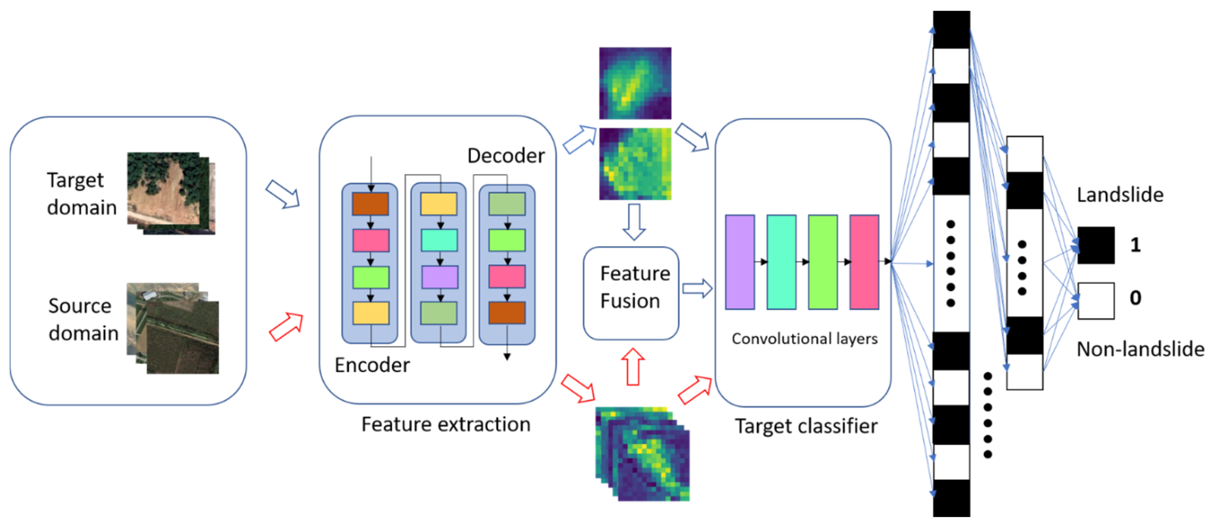
An important problem in transfer learning that has not been well studied is the fact that conventional transfer learning algorithms assume that the source domain and the target domain should be similar. For the landslide detection task of Longgang District, there are no similar open landslide datasets that can be used [57]. Therefore, we first introduce the novel feature-based distant domain transfer learning algorithm (DDTL), which requires only a small set of labeled target data and unlabeled source data from completely different domains [34,52,58]. The DDTL model contains two main modules, a feature extractor and a target classifier, and the structure of DDTL is shown in Figure 4. Moreover, we innovatively added the attention mechanism to the DDTL (AM-DDTL) and improved the attention model to make it more suitable for remote sensing landslide detection tasks.
In this paper, the AM-DDTL algorithm can solve the Longgang landslide detection problem in which there is no dataset similar to the target domain given the uniqueness of landslides. To the best of our knowledge, this is the first time that AM-DDTL has been applied to the field of landslide detection.
In the AM-DDTL problem, we assume that the Longgang target domain is too scarce to train a robust classification model. The source domain for the Longgang landslide dataset is insufficient.
In the AM-DDTL algorithm, we select other remote sensing datasets as the source domains denoted as S = {( x 1 1 , , x 1 n ), , ( x S N 1 , , x S N n )}, where n and S N represent the number of samples in each source domain and the number of source domains, respectively. Then, we have one labeled target domain denoted as T = {[( x 1 1 , y 1 1 ), , ( x 1 n , y 1 n )], , [ ( x T N 1 , y T N 1 ) , , ( x T N n , y T N n ) ] }, where n and T N represent the number of samples in each target domain and the number of target domains, respectively. Let P(x) and P(y|x) be the marginal and conditional distributions of a dataset, respectively. In the AM-DDTL problem, we have the following equations.
P S 1 ( x ) P S 2 ( x ) P S N ( x ) P T 1 ( x ) P T 2 ( x ) P T N ( x )
P T 1 ( y | x ) P T 2 ( y | x ) P T N ( y | x )
In this section, we introduce the convolutional autoencoder and the attention mechanisms separately; then, we explain how to evaluate the classification results. The framework of the DDTL is shown in Figure 5.

3.2.1. Autoencoder

The autoencoder first transforms the input information into a lower-dimensional representation and then reconstructs the initial input information using the lower-dimensional representation in the decoder part [59]. As an autoencoder trained on an unsupervised model can extract useful features from unlabeled data, deep learning models with autoencoders or unsupervised methods have been widely used in image and natural language processing [60].
The convolutional autoencoder with convolutional layers is suitable for the landslide detection task because the study area has only a few labeled landslide images that can be used. Therefore, the convolutional autoencoder can be used for feature extraction for the target landslide images and the source domain remote sensing images in the model.
The convolutional autoencoder, a kind of feed-forward neural network, is often used to solve image processing problems. The convolutional autoencoder consists of three main components, the encoder E c o n v ( · ) ,   the decoder D c o n v ( · ) and the loss function, which can measure the information loss due to compression. The encoder and the decoder of the convolutional autoencoder contain an input layer, convolutional layers and the output layer separately. The convolutional autoencoder is shown in Figure 6. The mechanism of the autoencoder can be expressed as follows:
f s = E c o n v ( X s ) , X s ^ = D c o n v ( f s )
where X s is the input image, f s is the image feature, and X s ^ is the output image.

3.2.2. Attention Mechanism

In convolutional neural networks for computer vision or natural language processes, attention modules that imitate human visual attention are very popular. We introduce the attention module to the DDTL framework to improve the transfer ability.
The squeeze-and-excitation (SE) module is a novel architectural unit [36]. The SE module focuses on the channel relationship of the given input feature map F i n R c × h × w to improve the performance of useful information extraction from the feature map. The SE model contains a squeeze operation M s q , excitation operation M e x and scale operation   M s c . The squeeze operation compresses the feature map F i n R c × h × w to a one-dimensional feature map F s q R c × 1 × 1 by global average pooling. After the squeeze operation, the one-dimensional feature maps F s q are passed through an excitation operation, which produces a set of weights F e x R c × 1 × 1   for every channel. The weights are applied to the feature map F i n at the scale operation, and the output F o u t of these operations is the outcome of the SE module, which can be directly passed into the other convolution layers of the networks.
The operation of the SE module is shown as follows.
F o u t = F i n Θ M s c ( M e x ( M s q ( F i n ) ) ) .  
where the symbol Θ denotes element-wise multiplication in this paper.
Unlike the SE module, the convolutional block attention module (CBAM) is an effective attention module for image recognition using convolutional neural networks in computer vision tasks [35]. This module handles the input features of the image along the two separate dimensions sequentially, the channel attention module and the spatial attention module, to help the information to flow within the network by learning which information to emphasize or suppress.
F o u t = F i n Θ M c ( F i n ) Θ M s ( F i n Θ M c ( F i n ) ) .  
To improve the performance of the DDTL framework for remote sensing image classification, we propose an improved attention module based on CBAM (improved CBAM). The improved attention module adapts the remote sensing image recognition and classification task well. On the basis of the CBAM module, inspired by the 3D spatial-channel attention module [61], we added a submodule to improve the extraction capacity of the input feature map. The improved attention module is different from the 3D spatial-channel attention module. For the improved attention module, the channel attention and spatial attention are connected in series. However, for the 3D spatial-channel attention module, the channel attention and spatial attention are connected in parallel. As shown in Figure 7, there are three convolution layers, with kernel sizes of 1 × 1, 3 × 3 and 7 × 7. The feature map F o u t from the CBAM module is sent into the submodule and then processed separately by 3 convolutional layers. After the outputs of the three convolutions are concatenated, a convolutional layer with a 7 × 7 kernel size follows the submodule.
F o u t = f 3 7 × 7 [ f 2 1 × 1 ( f 1 1 × 1 ( F o u t ) ) ; f 2 3 × 3 ( f 1 1 × 1 ( F o u t ) ) ; f 2 7 × 7 ( f 1 1 × 1 ( F o u t ) ) ]
where the F o u t is the outcome of the improved CBAM model and the F o u t is the outcome of the CBAM model. The f is the convolution operator and 1 × 1 denotes the kernel size.

3.2.3. The Loss of the Model

Three types of loss evaluation functions are used in the AM-DDTL framework: reconstruction loss, domain loss and classification loss. These loss functions are very important for the model to obtain a better classification result without large domain loss between the target and source domains and reconstruction loss of the autoencoder.

1. Reconstruction Loss

The reconstruction loss function is used to evaluate the difference between the input and output images of the convolutional autoencoder. After the images from the target and source domains are processed by the autoencoder, we define the reconstruction errors between the original images and the processed images as the loss function of the feature extractor L R . It is necessary to ensure that the difference between the input and output is small enough to obtain better extracted features. L R is given as follows:
L R = i = 1 S N j = 1 n S i 1 n S i ( X X S i j ^ X X S i j ) 2 + i = 1 S T j = 1 n T i 1 n T i ( X X T i j ^ X X T i j ) 2
where S N and S T are the number of source domains and target domains, respectively, and n S i and n T i are the number of instances in the source domain and target domain, respectively.   X X S i j ^ and X X T i j ^ are the reconstruction of the jth instances in the ith source domain and the target domain respectively. X X S i j and X X T i j are the jth instances in the ith source domain and the target domain, respectively.

2. Domain Loss

Usually, minimizing the reconstruction error L R can uncover the high-level features of the images. However, the distribution mismatch between the source and the target domains cannot be ignored, so only minimizing L R is not sufficient to obtain a robust model. To extract the same or similar features shared by the target domain and the source domain, we can minimize the domain distance between these domains. In other words, it is necessary to solve the problem of the distribution mismatch between the target and source domains, and we use the domain loss function to constrain the problem. The transfer model adds an adaptation layer to the convolutional autoencoder in order to measure the domain loss L D between the target domain and the source domain [62].
Regarding the domain loss L D , we use the maximum mean discrepancy (MMD) [63], an important statistical domain distance estimator, to measure the domain distance. The domain loss is expressed as follows:
L D = M M D ( i = 1 S N j = 1 n S i f S i j , i = 1 S T j = 1 n T i f T i j ) ,
M M D ( X , Y ) = | | 1 n 1 i = 1 n 1 φ ( x i ) + 1 n 2 f = 1 n 2 φ ( y i ) | | ,
where n 1   and n 2 are the numbers of instances of two different domains, and φ ( · ) is the kernel that converts two sets of features to a common reproducing kernel Hilbert space (RKHS), where the distance of two domains is maximized.

3. Classification Loss

After the encoder process, the high-level features extracted from the target domain are used for target classification with two fully connected layers. The fully connected layers can find the best feature combination for each class in the target task [64]. In the DDTL model, the output layer with a cross-entropy function is used to calculate the classification loss as follows:
L C = x [ C l a s s ] + i = 1 T N j = 1 n T i exp ( X T i j ) .

4. The Total Loss of the DDTL

According to the above three loss functions, the total loss is defined as follows:
min p E , p D , p C L = L R + L D + L C
where p E , p D ,   p C are the parameters of the encoder, decoder and classifier, respectively.
The framework of the proposed AM-DDTL model is shown in Figure 8.

4. Results

In this section, we first present the outcome of image enhancement and introduce the improved CBAM DDTL model. Then, we present an overview of the different attention mechanism comparison results. In addition, we explore the different effects of different source domains in obtaining a more accurate classification model using landslide remote sensing images.

4.1. The Result of Image Enhancement

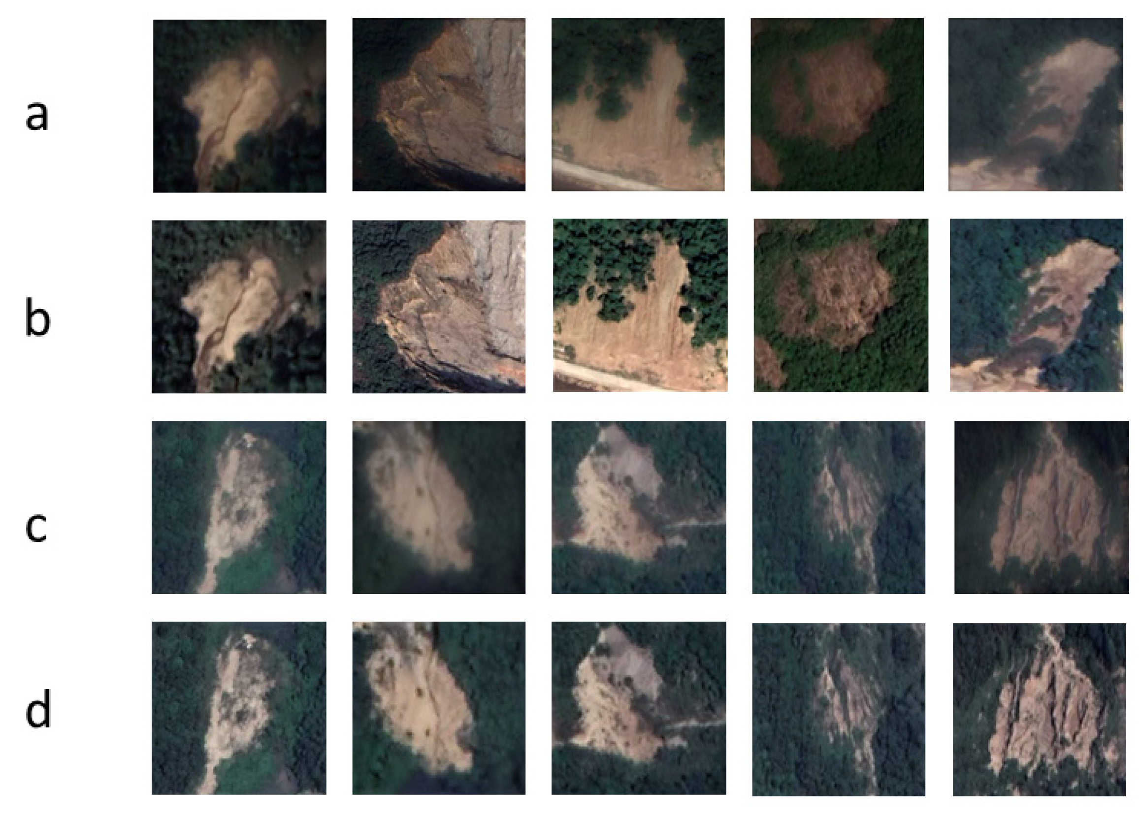
In this study, we processed optical images using illumination estimation techniques with a weight matrix and synthesized multiple exposure images using a camera response model [50]. The original high-resolution images extracted from Google Earth (Google Inc.) and the image-enhanced images are shown in Figure 9. Moreover, we conducted several experiments to explore the effect of image enhancement using different deep learning methods.
The enhanced images had good visual quality, and the image enhancement algorithm not only improved the brightness of the images but also made the details of the images clearer than before. Landslides have a strong contrast with the surrounding environment in remote sensing images.
To determine whether the image enhancement algorithm is useful for deep learning and computer vision, we compared the different deep learning methods using the enhanced images and the original images. The result is shown in Table 2. We can see that the experiment using enhanced images obtained higher accuracy than that using the original images.

4.2. The Comparison of Different Models

4.2.1. Landslide Detection by Pretrained Model

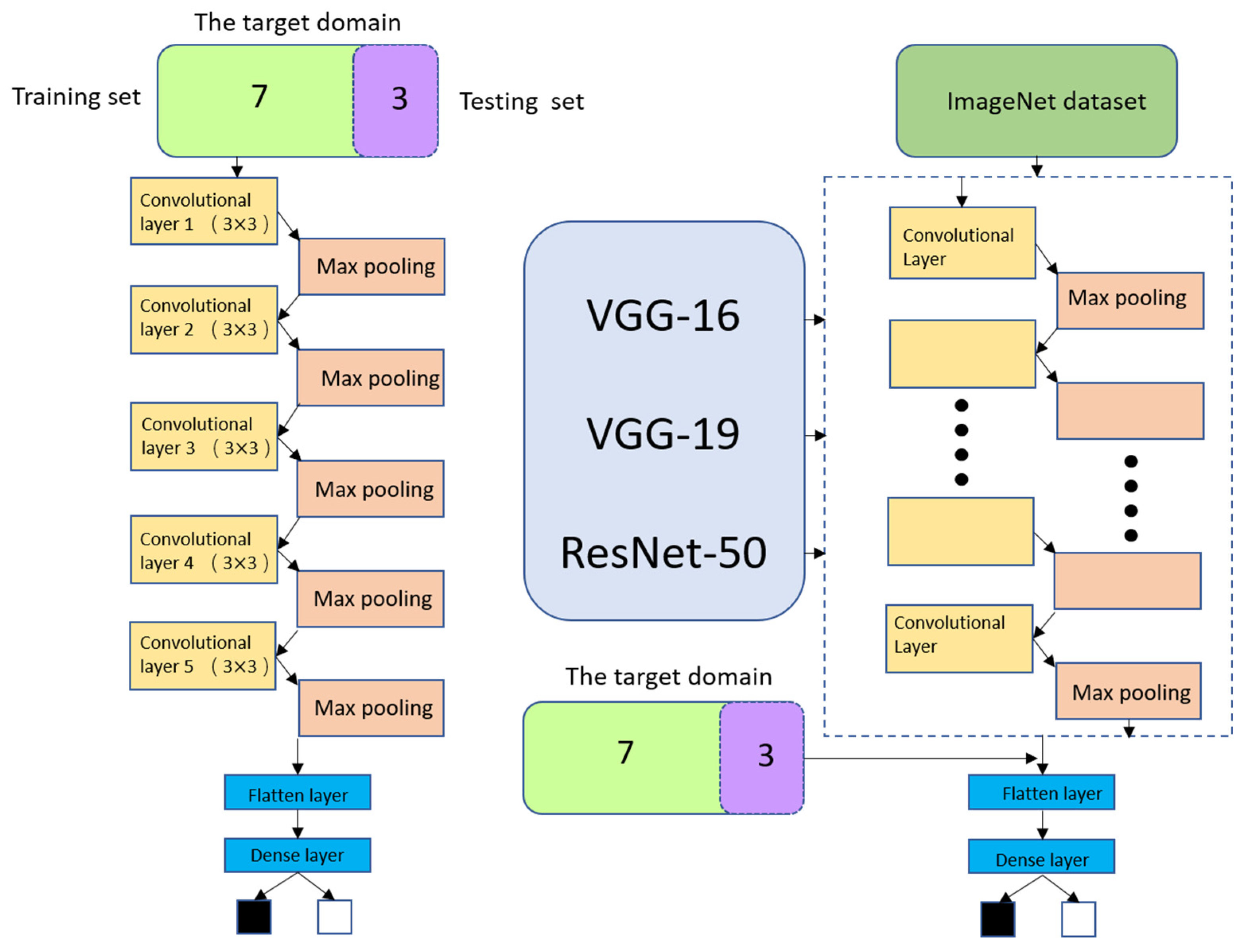
The most popular algorithm of traditional transfer learning is the pretrained model [65,66]. The pretrained models are trained by the ImageNet dataset [64,67,68] and then applied to the other image classifications, which can always reduce the time consumed and improve work efficiency. In other words, the target domain classification model is obtained by removing the top neural network of the existing ImageNet training model and retraining an output layer with the target domain. The structure of the pretrained model is shown in the right-hand picture in Figure 10.

4.2.2. Landslide Detection by the CNN Model

The convolutional neural network is widely used to solve image classification problems and is one of the most popular deep learning algorithms [18]. Compared with traditional machine learning algorithms, it has outstanding ability in image classification because of the convolution layers and subsampling layers, which can effectively extract the useful feature maps of images [64,69,70,71].
In this study, we constructed the CNN model with five convolutional layers with 3 × 3 kernels followed by a max-pooling kernel. The bottom of the convolutional neural network is connected with the flattened layer and the dense layers. The convolutional layer and the max-pooling layer can find and preserve the features of the image for classification, and the activation function sigmoid of the dense layers is excellent for binary classification. The structure of the normal CNN model is shown in the left-hand picture in Figure 10.
As shown in Table 2, DDTL achieved the highest accuracy (88.01%) for the classification task, but the CNN model only achieved 86.16% classification accuracy because the training data were insufficient [18]. Moreover, the pretrained models, VGG-16, VGG-19 and ResNet-50, achieved accuracies of 87.09% ~ 89.86%. The pretrained models achieved higher accuracy because these models were trained on a massive number of images and obtained the initial parameters. The settings of the pretrained model were more similar to those of the DDTL model; however, the accuracy of the pretrained model was lower than that of the DDTL model. The difference in the classification accuracy may have been caused by the different domain statistical distributions. In other words, the massive images used to train the pretrained models and Longgang landslide datasets had different distributions.
We used the remote sensing images (RGB) and DEM data of the Bijie landslide dataset as the source domain to explore the effect of DEM data on the landslide classification task. As shown in Table 3, the total loss of DDTL with RGB + DEM was lower compared with the results of RGB, and the result of classification using only DEM data was the worst. Therefore, in the experiments in this study, we used the DEM as the supplementary geomorphological data for the source domain.

4.3. The Comparison of Different Attention Mechanisms

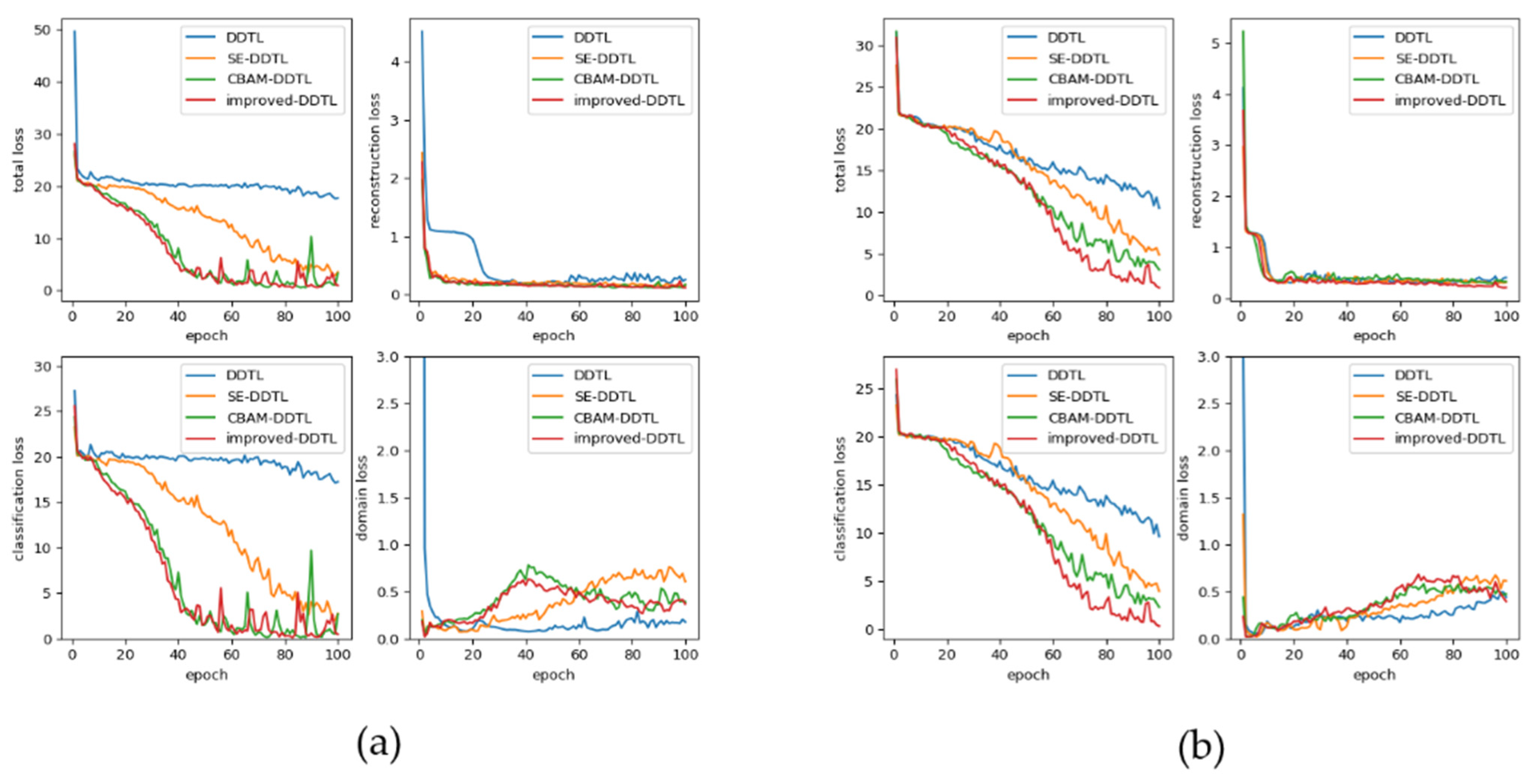
We improved a special attention mechanism based on the CBAM attention mechanism, and the improved CBAM was found to be suitable for information extraction from satellite images. Additionally, we compared the SE, CBAM and improved CBAM to obtain a better understanding of the effect of the attention mechanism. The outcome is shown in Figure 11 and Table 4.
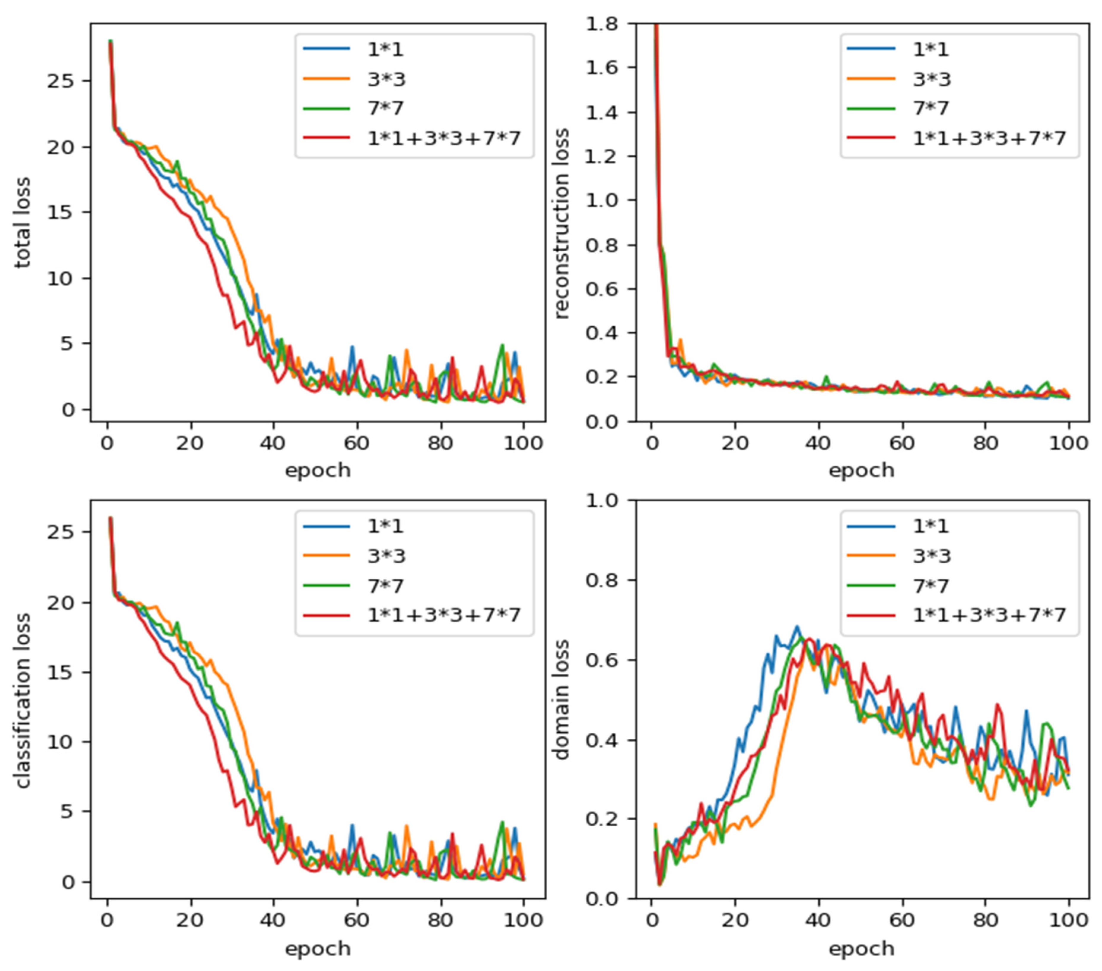
Regarding the improved attention mechanism, based on the CBAM attention mechanism, we added a submodule consisting of convolutional layers with different kernel sizes to extract more effective information. The submodule consists of three parallel convolutional layer subblocks that can process the information with the three convolutional layers. The three convolutional layers have different kernel sizes, 1 × 1, 3 × 3 and 7 × 7, which can extract the characteristics of landslides from different scales. To select and verify the subblock’s structure, we compared the effect of the different kernel sizes. Figure 12 shows that the three parallel convolutional layer subblocks produce the best classification effect. In addition, the convolutional layer with a kernel size of 1 × 1 also achieves better performance because this kernel size can extract the information from each pixel of the feature map, but this capability may extract more useless information.
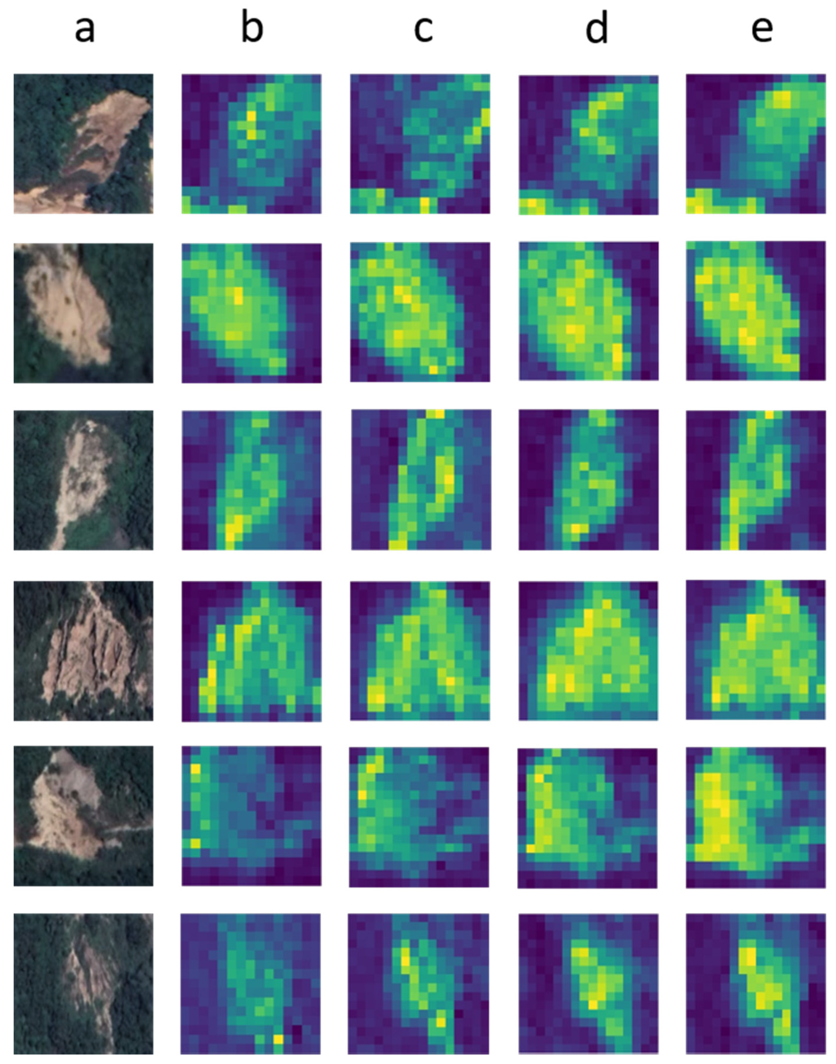
We obtained feature maps with different attention mechanisms in the DDTL model: the SE-DDTL module, the CBAM-DDTL module and the improved CBAM-DDTL module. We compared the landslide image produced using these models, and the outcome of the comparison is shown in Figure 13. We found that the feature map of CBAM-DDTL and the improved CBAM-DDTL produced good landslide feature performance. The normal DDTL model without an attention mechanism always obtained a few landslide feature pixels, and the feature extraction effect of the SE-DDTL model was between that of DDTL without an attention mechanism and DDTL with CBAM. In later experiments, we used the improved CBAM-DDTL as the model.

4.4. The Comparison of Different Source Domains

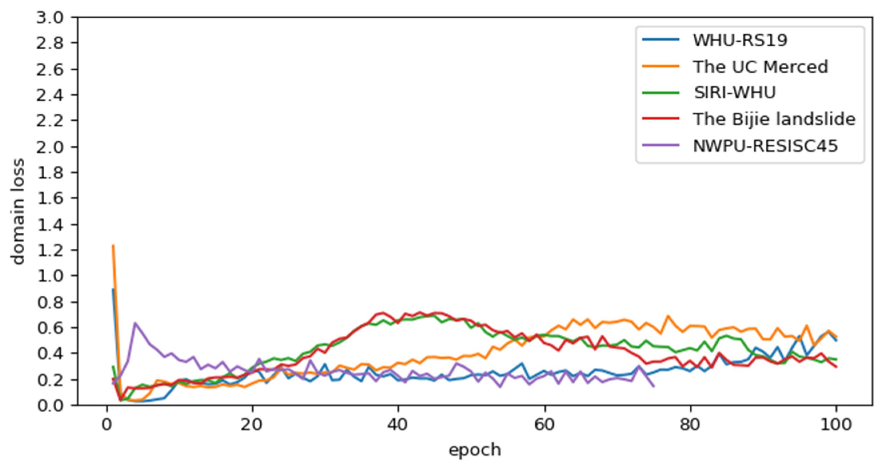
In this section, we first compare the different source domains, as shown in Figure 14 and Figure 15. We selected five datasets: WHU-RS19 dataset, the UC Merced land use dataset, the Google Earth dataset of SIRI-WHU, the Bijie landslide dataset and the NWPU-RESISC45 dataset. They differ in the number and variety of remote sensing images. First, the NWPU-RESISC45 dataset achieves the best performance not only in terms of the classification loss but also the total loss. In addition to gaining the lowest loss values, the curve of the NWPU-RESISC45 dataset is smoother than that of the other source domains. Using the NWPU-RESISC45 dataset as the source domain, the model needs less than twenty epochs to reach equilibrium, while, for the other source domains, the model may need more than 40 cycles to obtain a good result. However, the Bijie landslide dataset did not achieve the best performance, although it was visually more similar to the Longgang landslide dataset. The SIRI-WHU and Bijie landslide datasets had the same training curve and achieved a well-trained state at the same time, but the curve of the Bijie landslide dataset had some unstable values and larger fluctuations. The UC Merced land use dataset’s training curve finally started to stabilize, but for WHU-RS19, training still continued after 100 epochs.
Regarding the domain loss of different source domains, as shown in Figure 15, the domain loss of the NWPU-RESISC45 dataset first increases and then tends towards the lowest stable value state. The domain loss of the WHU-RS19 dataset continues to rise because the training is ongoing. The SIRI-WHU and Bijie landslide datasets share the same curve shape for domain loss.
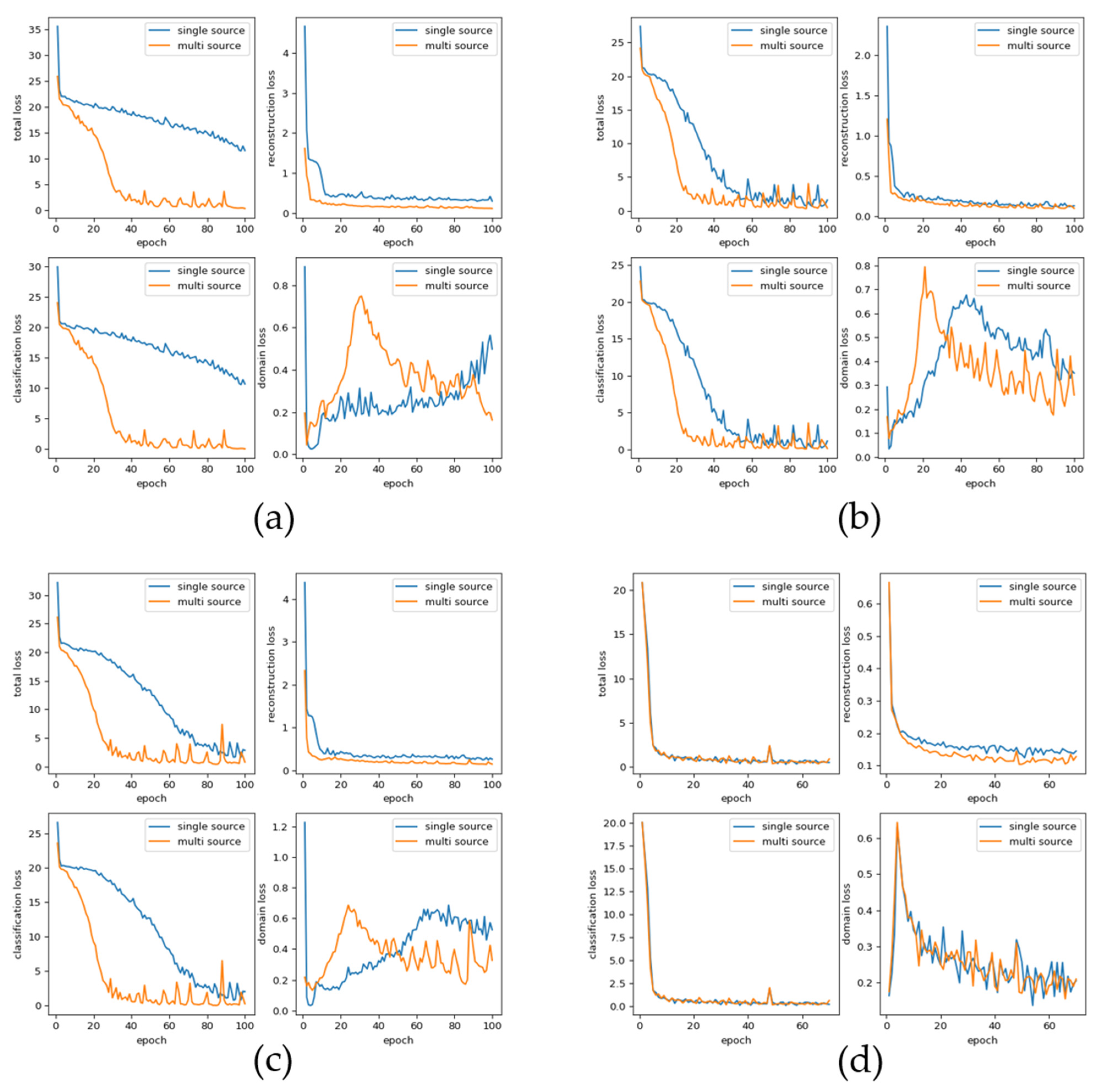
After comparing the differences in the single source domains, we also explored the best combination of these source domains because the high-level features of different source domains are different, and they may overlap or intersect. For this purpose, we compared the single domain with the multisource domain to explore the effects of these remote sensing image datasets and found the optimal source domain combination that could obtain the best classification effect for landslide images. The outcome of this experiment is shown in Figure 16.
Figure 16 and Table 5 shows that NWPU-RESISC45 obtains the best classification effect, whether acting as the single source domain or combined with the Bijie landslide dataset, and the two curves are highly coincident. The most obvious result is the substantial improvement in the classification effect when the three remote sensing scene classification datasets, WHU-RS19, the UC Merced land use dataset and SIRI-WHU, are combined with the Bijie landslide dataset. Especially for the WHU-RS19 dataset, using the single WHU-RS19 source, the model did not achieve a stable state, while the model using the multisource model obtained a better effect when trained only approximately 40 times. For the other two datasets, the gap between the two curves in the total loss represents the improvement of the classification effect.
For the domain loss, the UC Merced land use dataset and the SIRI-WHU dataset are consistent, and the two curves of single source and multisource gradually stabilize after rising, although the number of training sessions is different. In addition, comparing the curves of the SIRI-WHU dataset and the UC Merced land use dataset shows that the two curves of the SIRI-WHU dataset are more similar in shape than those of the UC Merced land use dataset.

4.5. Effectiveness Verification of Landslide Detection

In order to verify the effect of the landslide detection model, we evaluated whether the model could identify the landslides and further aid in indoor remote sensing interpretation work. The northern region of Longgang, having a more complex terrain environment, was used as the verification area. Here, there may have been undiscovered or recently occurring landslides. We applied our improved CBAM-DDTL model using the Bijie landslide dataset and NWPU-RESISC45 as the source domain. Finally, the model found 12 suspicious landslide candidates.
After the targeted detailed investigations in the field, the 12 candidates were confirmed by the authors. This demonstrated that more than 95% of the candidates were real landslides. The verification experiment in this area showed that our proposed landslide detection model provides outstanding performance.

5. Discussion

In this study, we compared the CNN model, pretrained model and DDTL method. The CNN model obtained the worst classification accuracy, and the DDTL model and the pretrained model obtained similar classification results, which were better than those of the CNN model.
Regarding the CNN model and the pretrained model, we used the Longgang landslide dataset, which only contains 177 landslide images, to train the classification model, and we divided the whole landslide dataset into a training set and validation set according to the ratio of 7:3, as in previous research [1,71]. After multiple training steps, we obtained the training results. We conclude that the CNN model did not obtain promising classification results because only a few images were used for its training, and the CNN model could not extract useful features for landslide classification. The pretrained model obtained similar classification results as the DDTL model because these pretrained models have initial parameters trained on massive images. The pretrained model can extract the high-level feature maps of the remote sensing images. However, after intensive study, we found that the massive images used to train the model had a mismatch distribution with the target, the Longgang landslide dataset, which may have influenced the classification effect. The pre-obtained parameters can alleviate the shortcomings to obtain better results.
In this paper, we innovatively introduce an attention mechanism into distant domain transfer learning because remote sensing landslide images contain complex information, such as rivers, roads and lakes. This redundant information may harm landslide classification. Therefore, we introduce the attention mechanism into the convolution process for feature extraction. The SE attention mechanism extracts the deep landslide image features through channel attention. The CBAM attention mechanism, unlike the SE mechanism, extracts a feature through the channel and the spatial attention and obtains good feature extraction. Therefore, the classification of CBAM-DDTL has better accuracy than the SE-DDTL model. Regarding the improved CBAM-DDTL model inspired by [61], we process the outcome of the CBAM with three parallel convolutional layers with kernel sizes of 1 × 1, 3 × 3 and 7 × 7. To verify the effect of the subblock with three parallel convolutional layers, we compared the classification effect for kernel sizes of 1 × 1, 3 × 3 and 7 × 7, and the three parallel convolutional layers. The parallel convolutional layers obtained the lowest total loss—the result is the same as the outcome of [6]—and we conclude that the reason is that the 1 × 1 kernel size layer can discover small pixels of high features, and paralleling with another two kernel size layers can slightly increase the extraction effect.
Regarding the source domains, the NWPU-RESISC45 source domain obtains the lowest total loss, while WHU-RS19 obtains the worst performance. Therefore, the quantity and diversity of the source domain is the dominant factor for the classification effect. In addition, we know that the domain distance is smaller when the domain loss is lower, as with medical image classification [58], because, as Figure 16 shows, the combination of NWPU-RESISC45 and the Bijie landslide dataset results in not only the lowest total loss but also the lowest domain loss.
From Figure 14, we can easily see that the Bijie landslide dataset does not achieve the best results. Therefore, we can conclude that the source domain is visually similar to the target domain, and the classification results may not be optimal. The SIRI-WHU and Bijie landslide datasets have the same performance and approximately the same number of images. Moreover, in Figure 16, the two domain loss curves of a single source and multiple sources have the same shape, which shows that the two datasets share a certain number of high-level features.
Comparing the UC Merced land use dataset with the Bijie landslide dataset shows that the Bijie landslide dataset has more common features with the target domain than the UC Merced land use dataset and can obtain a more stable classification loss value sooner. For the UC Merced land use dataset, the convolution operation continuously extracts deep features common to the target domain, and the model obtains a small classification loss. This is because the feature map of the Bijie landside dataset is more similar to the Longgang landslide target domain than the UC Merced land use dataset.
The study in this paper has two limitations: (1) the feature extraction of remote sensing images using the DDTL algorithm is computationally expensive; (2) the landslide classification task also needs a publicly available landslide remote sensing dataset with a huge number of images for further research; (3) due to some limitations, we cannot use high-resolution remote sensing satellite images such as the Gaofen series and only use Google Earth images for analysis.

6. Conclusions

In this paper, we introduce the DDTL algorithm for landslide detection in the Longgang District based on remote sensing images and highly accurate DEM. Three contributions make this study distinctive. First, we innovatively introduce the DDTL algorithm. The DDTL algorithm does not require training data and testing data to have the same probability distribution, and it can handle the classification task, which only has a few labeled target samples, by transferring knowledge from completely different source domains. Second, we combine the attention mechanism and the DDTL algorithm and propose an improved attention mechanism that is suitable for landslide detection. Third, this is the first study to introduce scene classification datasets into the landslide detection task. We use the classification loss, reconstruction loss and domain loss to evaluate the DDTL model. All the experimental results show that the improved CBAM-DDTL has a better classification effect than other methods, and the NWPU-RESISC45 dataset is more suitable than other datasets for the landslide detection task using the DDTL model.

Author Contributions

Conceptualization, S.Q. (Shengwu Qin) and X.G.; methodology, X.G.; software, X.G.; validation, J.S., S.Q. (Shuangshuang Qiao), X.G., Y.Z. and Q.C.; formal analysis, J.Y.; investigation, J.Y. and J.S.; resources, L.Z.; data curation, X.G.; writing—original draft preparation, X.G.; writing—review and editing, X.G. and J.S., S.Q. (Shuangshuang Qiao); visualization, X.G.; supervision, S.Q. (Shengwu Qin); project administration, S.Q. (Shengwu Qin); funding acquisition, S.Q. (Shengwu Qin). All authors have read and agreed to the published version of the manuscript.

Funding

This research was funded by the National Natural Science Foundation of China (Grant Nos. 41977221, 41972267 and 41202197) and the Jilin Provincial Science and Technology Department (Grant Nos. 20190303103SF and 20170101001JC).

Institutional Review Board Statement

Not applicable.

Informed Consent Statement

Not applicable.

Data Availability Statement

The Bijie Landsldie dataset is available at http://gpcv.whu.edu.cn/data/ (accessed on 22 June 2021).

Conflicts of Interest

The authors declare no conflict of interest.

References

  1. Mohan, A.; Singh, A.K.; Kumar, B.; Dwivedi, R. Review on remote sensing methods for landslide detection using machine and deep learning. Trans. Emerg. Telecommun. Technol. 2020, 32, e3998. [Google Scholar] [CrossRef]
  2. Iverson, R.M. Landslide triggering by rain infiltration. Water Resour. Res. 2000, 36, 1897–1910. [Google Scholar] [CrossRef] [Green Version]
  3. Haque, U.; da Silva, P.F.; Devoli, G.; Pilz, J.; Zhao, B.; Khaloua, A.; Wilopo, W.; Andersen, P.; Lu, P.; Lee, J.; et al. The human cost of global warming: Deadly landslides and their triggers (1995–2014). Sci. Total Environ. 2019, 682, 673–684. [Google Scholar] [CrossRef]
  4. Zhou, S.Y.; Gao, L.; Zhang, L.M. Predicting debris-flow clusters under extreme rainstorms: A case study on Hong Kong Island. Bull. Eng. Geol. Environ. 2019, 78, 5775–5794. [Google Scholar] [CrossRef]
  5. Hölbling, D.; Füreder, P.; Antolini, F.; Cigna, F.; Casagli, N.; Lang, S. A Semi-Automated Object-Based Approach for Landslide Detection Validated by Persistent Scatterer Interferometry Measures and Landslide Inventories. Remote Sens. 2012, 4, 1310–1336. [Google Scholar] [CrossRef] [Green Version]
  6. Ji, S.; Yu, D.; Shen, C.; Li, W.; Xu, Q. Landslide detection from an open satellite imagery and digital elevation model dataset using attention boosted convolutional neural networks. Landslides 2020, 17, 1337–1352. [Google Scholar] [CrossRef]
  7. Miele, P.; Di Napoli, M.; Guerriero, L.; Ramondini, M.; Sellers, C.; Corona, M.A.; Di Martire, D. Landslide Awareness System (LAwS) to Increase the Resilience and Safety of Transport Infrastructure: The Case Study of Pan-American Highway (Cuenca-Ecuador). Remote Sens. 2021, 13, 1564. [Google Scholar] [CrossRef]
  8. Qi, T.J.; Zhao, Y.; Meng, X.M.; Chen, G.; Dijkstra, T. AI-Based Susceptibility Analysis of Shallow Landslides Induced by Heavy Rainfall in Tianshui, China. Remote Sens. 2021, 13, 1819. [Google Scholar] [CrossRef]
  9. Liu, B.; He, K.; Han, M.; Hu, X.W.; Ma, G.T.; Wu, M.Y. Application of UAV and GB-SAR in Mechanism Research and Monitoring of Zhonghaicun Landslide in Southwest China. Remote Sens. 2021, 13, 1653. [Google Scholar] [CrossRef]
  10. Pham, B.T.; Prakash, I.; Jaafari, A.; Bui, D.T. Spatial Prediction of Rainfall-Induced Landslides Using Aggregating One-Dependence Estimators Classifier. J. Indian Soc. Remote Sens. 2018, 46, 1457–1470. [Google Scholar] [CrossRef]
  11. Xie, M.; Jean, N.; Burke, M.; Lobell, D.; Ermon, S. Transfer Learning from Deep Features for Remote Sensing and Poverty Mapping; Assoc Advancement Artificial Intelligence: Palo Alto, CA, USA, 2016; pp. 3929–3935. [Google Scholar]
  12. Qiao, S.; Qin, S.; Chen, J.; Hu, X.; Ma, Z. The Application of a Three-Dimensional Deterministic Model in the Study of Debris Flow Prediction Based on the Rainfall-Unstable Soil Coupling Mechanism. Processes 2019, 7, 99. [Google Scholar] [CrossRef] [Green Version]
  13. Sun, J.; Qin, S.; Qiao, S.; Chen, Y.; Su, G.; Cheng, Q.; Zhang, Y.; Guo, X. Exploring the impact of introducing a physical model into statistical methods on the evaluation of regional scale debris flow susceptibility. Nat. Hazards 2021, 106, 881–912. [Google Scholar] [CrossRef]
  14. Yao, J.; Qin, S.; Qiao, S.; Che, W.; Chen, Y.; Su, G.; Miao, Q. Assessment of Landslide Susceptibility Combining Deep Learning with Semi-Supervised Learning in Jiaohe County, Jilin Province, China. Appl. Sci. 2020, 10, 5640. [Google Scholar] [CrossRef]
  15. Bui, D.T.; Tsangaratos, P.; Nguyen, V.-T.; Liem, N.V.; Trinh, P.T. Comparing the prediction performance of a Deep Learning Neural Network model with conventional machine learning models in landslide susceptibility assessment. Catena 2020, 188, 104426. [Google Scholar] [CrossRef]
  16. Ding, A.; Zhang, Q.; Zhou, X.; Dai, B. Automatic recognition of landslide based on CNN and texture change detection. In Proceedings of the 2016 31st Youth Academic Annual Conference of Chinese Association of Automation (YAC), Wuhan, China, 11–13 November 2016; pp. 444–448. [Google Scholar]
  17. Yang, B.; Wang, S.; Zhou, Y.; Wang, F.; Hu, Q.; Chang, Y.; Zhao, Q. Extraction of road blockage information for the Jiuzhaigou earthquake based on a convolution neural network and very-high-resolution satellite images. Earth Sci. Inform. 2019, 13, 115–127. [Google Scholar] [CrossRef]
  18. Ghorbanzadeh, O.; Blaschke, T.; Gholamnia, K.; Meena, S.; Tiede, D.; Aryal, J. Evaluation of Different Machine Learning Methods and Deep-Learning Convolutional Neural Networks for Landslide Detection. Remote Sens. 2019, 11, 196. [Google Scholar] [CrossRef] [Green Version]
  19. Prakash, N.; Manconi, A.; Loew, S. Mapping Landslides on EO Data: Performance of Deep Learning Models vs. Traditional Machine Learning Models. Remote Sens. 2020, 12, 346. [Google Scholar] [CrossRef] [Green Version]
  20. Sameen, M.I.; Pradhan, B. Landslide Detection Using Residual Networks and the Fusion of Spectral and Topographic Information. IEEE Access 2019, 7, 114363–114373. [Google Scholar] [CrossRef]
  21. Wang, Y.; Wang, X.; Jian, J. Remote Sensing Landslide Recognition Based on Convolutional Neural Network. Math. Probl. Eng. 2019, 2019, 1–12. [Google Scholar] [CrossRef]
  22. Liu, T.; Abd-Elrahman, A.; Morton, J.; Wilhelm, V.L. Comparing fully convolutional networks, random forest, support vector machine, and patch-based deep convolutional neural networks for object-based wetland mapping using images from small unmanned aircraft system. GISci. Remote Sens. 2018, 55, 243–264. [Google Scholar] [CrossRef]
  23. Ghorbanzadeh, O.; Meena, S.R.; Blaschke, T.; Aryal, J. UAV-Based Slope Failure Detection Using Deep-Learning Convolutional Neural Networks. Remote Sens. 2019, 11, 2046. [Google Scholar] [CrossRef] [Green Version]
  24. Shawky, O.A.; Hagag, A.; El-Dahshan, E.-S.A.; Ismail, M.A. Remote sensing image scene classification using CNN-MLP with data augmentation. Optik 2020, 221, 165356. [Google Scholar] [CrossRef]
  25. Censi, A.M.; Ienco, D.; Gbodjo, Y.J.E.; Pensa, R.G.; Interdonato, R.; Gaetano, R. Attentive Spatial Temporal Graph CNN for Land Cover Mapping from Multi Temporal Remote Sensing Data. IEEE Access 2021, 9, 23070–23082. [Google Scholar] [CrossRef]
  26. Zhu, H.; Xie, C.; Fei, Y.; Tao, H. Attention Mechanisms in CNN-Based Single Image Super-Resolution: A Brief Review and a New Perspective. Electronics 2021, 10, 1187. [Google Scholar] [CrossRef]
  27. Xu, R.; Tao, Y.; Lu, Z.; Zhong, Y. Attention-Mechanism-Containing Neural Networks for High-Resolution Remote Sensing Image Classification. Remote Sens. 2018, 10, 1602. [Google Scholar] [CrossRef] [Green Version]
  28. Chan, C.S.; Anderson, D.T.; Ball, J.E. Comprehensive survey of deep learning in remote sensing: Theories, tools, and challenges for the community. J. Appl. Remote Sens. 2017, 11, 042609. [Google Scholar] [CrossRef] [Green Version]
  29. Lu, H.; Ma, L.; Fu, X.; Liu, C.; Wang, Z.; Tang, M.; Li, N. Landslides Information Extraction Using Object-Oriented Image Analysis Paradigm Based on Deep Learning and Transfer Learning. Remote Sens. 2020, 12, 752. [Google Scholar] [CrossRef] [Green Version]
  30. Zhao, H.; Liu, F.; Zhang, H.; Liang, Z. Convolutional neural network based heterogeneous transfer learning for remote-sensing scene classification. Int. J. Remote Sens. 2019, 40, 8506–8527. [Google Scholar] [CrossRef]
  31. Pires de Lima, R.; Marfurt, K. Convolutional Neural Network for Remote-Sensing Scene Classification: Transfer Learning Analysis. Remote Sens. 2019, 12, 86. [Google Scholar] [CrossRef] [Green Version]
  32. Tan, B.; Zhang, Y.; Pan, S.J.; Yang, Q. Distant Domain Transfer Learning; Assoc Advancement Artificial Intelligence: Palo Alto, CA, USA, 2017; pp. 2604–2610. [Google Scholar]
  33. Tan, B.; Song, Y.; Zhong, E.; Yang, Q. Transitive Transfer Learning. In Proceedings of the 21th ACM SIGKDD International Conference on Knowledge Discovery and Data Mining, Sydney, Australia, 10–13 August 2015; pp. 1155–1164. [Google Scholar]
  34. Niu, S.; Hu, Y.; Wang, J.; Liu, Y.; Song, H. Feature-based Distant Domain Transfer Learning. In Proceedings of the 2020 IEEE International Conference on Big Data (Big Data), Atlanta, GA, USA, 10–13 December 2020; pp. 5164–5171. [Google Scholar]
  35. Woo, S.; Park, J.; Lee, J.-Y.; Kweon, I.S. CBAM: Convolutional Block Attention Module. In Proceedings of the Computer Vision—ECCV 2018, München, Germany, 8–14 September 2018; pp. 3–19. [Google Scholar]
  36. Hu, J.; Shen, L.; Albanie, S.; Sun, G.; Wu, E. Squeeze-and-Excitation Networks. IEEE Trans. Pattern Anal. Mach. Intell. 2020, 42, 2011–2023. [Google Scholar] [CrossRef] [Green Version]
  37. Jiang, G.G.; Tian, Y.; Xiao, C.C. GIS-based Rainfall-Triggered Landslide Warning and Forecasting Model of Shenzhen. In Proceedings of the 2013 21st International Conference on Geoinformatics, Kaifeng, China, 20–22 June 2013; Hu, S., Ye, X., Eds.; IEEE: New York, NY, USA, 2013. [Google Scholar]
  38. He, X.C.; Xu, Y.S.; Shen, S.L.; Zhou, A.N. Geological environment problems during metro shield tunnelling in Shenzhen, China. Arab. J. Geosci. 2020, 13, 1–18. [Google Scholar] [CrossRef]
  39. Guzzetti, F.; Peruccacci, S.; Rossi, M.; Stark, C.P. The rainfall intensity–duration control of shallow landslides and debris flows: An update. Landslides 2008, 5, 3–17. [Google Scholar] [CrossRef]
  40. Zhang, X.; Song, J.; Peng, J.; Wu, J. Landslides-oriented urban disaster resilience assessment-A case study in ShenZhen, China. Sci. Total Environ. 2019, 661, 95–106. [Google Scholar] [CrossRef] [PubMed]
  41. Luo, H.Y.; Shen, P.; Zhang, L.M. How does a cluster of buildings affect landslide mobility: A case study of the Shenzhen landslide. Landslides 2019, 16, 2421–2431. [Google Scholar] [CrossRef]
  42. Rau, J.-Y.; Jhan, J.-P.; Rau, R.-J. Semiautomatic Object-Oriented Landslide Recognition Scheme From Multisensor Optical Imagery and DEM. IEEE Trans. Geosci. Remote Sens. 2014, 52, 1336–1349. [Google Scholar] [CrossRef]
  43. Yang, Y.; Newsam, S. Bag-of-visual-words and spatial extensions for land-use classification. In Proceedings of the 18th SIGSPATIAL International Conference on Advances in Geographic Information Systems, San Jose, CA, USA, 2–5 November 2010; pp. 270–279. [Google Scholar]
  44. Zhao, B.; Zhong, Y.F.; Zhang, L.P.; Huang, B. The Fisher Kernel Coding Framework for High Spatial Resolution Scene Classification. Remote Sens. 2016, 8, 157. [Google Scholar] [CrossRef] [Green Version]
  45. Zhao, B.; Zhong, Y.F.; Xia, G.S.; Zhang, L.P. Dirichlet-Derived Multiple Topic Scene Classification Model for High Spatial Resolution Remote Sensing Imagery. IEEE Trans. Geosci. Remote Sens. 2016, 54, 2108–2123. [Google Scholar] [CrossRef]
  46. Cheng, G.; Han, J.; Lu, X. Remote Sensing Image Scene Classification: Benchmark and State of the Art. Proc. IEEE 2017, 105, 1865–1883. [Google Scholar] [CrossRef] [Green Version]
  47. Dai, D.; Yang, W. Satellite Image Classification via Two-Layer Sparse Coding with Biased Image Representation. IEEE Geosci. Remote Sens. Lett. 2011, 8, 173–176. [Google Scholar] [CrossRef] [Green Version]
  48. Wang, S.; Zheng, J.; Hu, H.; Li, B. Naturalness Preserved Enhancement Algorithm for Non-Uniform Illumination Images. IEEE Trans. Image Process. 2013, 22, 3538–3548. [Google Scholar] [CrossRef]
  49. Ibrahim, H.; Kong, N.S.P. Brightness Preserving Dynamic Histogram Equalization for Image Contrast Enhancement. IEEE Trans. Consum. Electron. 2007, 53, 1752–1758. [Google Scholar] [CrossRef]
  50. Ying, Z.Q.; Li, G.; Ren, Y.R.; Wang, R.G.; Wang, W.M. A New Image Contrast Enhancement Algorithm Using Exposure Fusion Framework. In Computer Analysis of Images and Patterns: 17th International Conference, Caip 2017, Pt II; Felsberg, M., Heyden, A., Kruger, N., Eds.; Springer International Publishing Ag: Cham, Switzerland, 2017; Volume 10425, pp. 36–46. [Google Scholar]
  51. Ying, Z.; Li, G.; Ren, Y.; Wang, R.; Wang, W. A New Low-Light Image Enhancement Algorithm Using Camera Response Model. In Proceedings of the 2017 IEEE International Conference on Computer Vision Workshops (ICCVW), Venice, Italy, 22–29 October 2017; pp. 3015–3022. [Google Scholar]
  52. Niu, S.; Liu, Y.; Wang, J.; Song, H. A Decade Survey of Transfer Learning (2010–2020). IEEE Trans. Artif. Intell. 2020, 1, 151–166. [Google Scholar] [CrossRef]
  53. Tan, B.; Yu, Z.; Pan, S.J.; Qiang, Y. Distant Domain Transfer Learning. In Proceedings of the AAAI Conference on Artificial Intelligence, San Francisco, CA, USA, 4–9 February 2017. [Google Scholar]
  54. Pan, S.J.; Yang, Q. A Survey on Transfer Learning. IEEE Trans. Knowl. Data Eng. 2010, 22, 1345–1359. [Google Scholar] [CrossRef]
  55. Tan, C.; Sun, F.; Kong, T.; Zhang, W.; Yang, C.; Liu, C. A Survey on Deep Transfer Learning. In Artificial Neural Networks and Machine Learning—ICANN 2018; Springer: Cham, Switzerland, 2018; pp. 270–279. [Google Scholar]
  56. Zhuang, F.; Qi, Z.; Duan, K.; Xi, D.; Zhu, Y.; Zhu, H.; Xiong, H.; He, Q. A Comprehensive Survey on Transfer Learning. Proc. IEEE 2021, 109, 43–76. [Google Scholar] [CrossRef]
  57. Notti, D.; Giordan, D.; Cina, A.; Manzino, A.; Maschio, P.; Bendea, I.H. Debris Flow and Rockslide Analysis with Advanced Photogrammetry Techniques Based on High-Resolution RPAS Data. Ponte Formazza Case Study (NW Alps). Remote Sens. 2021, 13, 1797. [Google Scholar] [CrossRef]
  58. Niu, S.; Liu, M.; Liu, Y.; Wang, J.; Song, H. Distant Domain Transfer Learning for Medical Imaging. IEEE J. Biomed. Health Inform. 2021, 21, 1-1. [Google Scholar] [CrossRef]
  59. Liu, Y.; Wu, L. Geological Disaster Recognition on Optical Remote Sensing Images Using Deep Learning. Procedia Comput. Sci. 2016, 91, 566–575. [Google Scholar] [CrossRef] [Green Version]
  60. Turchenko, V.; Chalmers, E.; Luczak, A. A Deep Convolutional Auto-Encoder with Pooling—Unpooling Layers in Caffe. arXiv 2017, arXiv:1701.04949. [Google Scholar]
  61. Catani, F. Landslide detection by deep learning of non-nadiral and crowdsourced optical images. Landslides 2020, 18, 1025–1044. [Google Scholar] [CrossRef]
  62. Sun, B.; Saenko, K. Deep CORAL: Correlation Alignment for Deep Domain Adaptation. In Proceedings of the Computer Vision—ECCV 2016 Workshops, Amsterdam, The Netherlands, 8–10 and 15–16 October 2016; pp. 443–450. [Google Scholar]
  63. Borgwardt, K.M.; Gretton, A.; Rasch, M.J.; Kriegel, H.-P.; Schoelkopf, B.; Smola, A.J. Integrating structured biological data by Kernel Maximum Mean Discrepancy. Bioinformatics 2006, 22, E49–E57. [Google Scholar] [CrossRef] [Green Version]
  64. Krizhevsky, A.; Sutskever, I.; Hinton, G.E. ImageNet classification with deep convolutional neural networks. Commun. ACM 2017, 60, 84–90. [Google Scholar] [CrossRef]
  65. Bai, S.; Wang, J.; Zhang, Z.; Cheng, C. Combined landslide susceptibility mapping after Wenchuan earthquake at the Zhouqu segment in the Bailongjiang Basin, China. Catena 2012, 99, 18–25. [Google Scholar] [CrossRef]
  66. Xu, C.; Xu, X.; Dai, F.; Wu, Z.; He, H.; Shi, F.; Wu, X.; Xu, S. Application of an incomplete landslide inventory, logistic regression model and its validation for landslide susceptibility mapping related to the May 12, 2008 Wenchuan earthquake of China. Nat. Hazards 2013, 68, 883–900. [Google Scholar] [CrossRef]
  67. Russakovsky, O.; Deng, J.; Su, H.; Krause, J.; Satheesh, S.; Ma, S.; Huang, Z.; Karpathy, A.; Khosla, A.; Bernstein, M.; et al. ImageNet Large Scale Visual Recognition Challenge. Int. J. Comput. Vis. 2015, 115, 211–252. [Google Scholar] [CrossRef] [Green Version]
  68. Deng, J.; Dong, W.; Socher, R.; Li, L.; Kai, L.; Li, F.-F. ImageNet: A large-scale hierarchical image database. In Proceedings of the 2009 IEEE Conference on Computer Vision and Pattern Recognition, Miami, FL, USA, 20–25 June 2009; pp. 248–255. [Google Scholar]
  69. Cheng, G.; Ma, C.; Zhou, P.; Yao, X.; Han, J. Scene classification of high resolution remote sensing images using convolutional neural networks. In Proceedings of the 2016 IEEE International Geoscience and Remote Sensing Symposium (IGARSS), Beijing, China, 10–15 July 2016; pp. 767–770. [Google Scholar]
  70. Tajbakhsh, N.; Shin, J.Y.; Gurudu, S.R.; Hurst, R.T.; Kendall, C.B.; Gotway, M.B.; Liang, J. Convolutional Neural Networks for Medical Image Analysis: Full Training or Fine Tuning? IEEE Trans. Med. Imaging 2016, 35, 1299–1312. [Google Scholar] [CrossRef] [Green Version]
  71. Chen, Y.; Qin, S.; Qiao, S.; Dou, Q.; Che, W.; Su, G.; Yao, J.; Nnanwuba, U.E. Spatial Predictions of Debris Flow Susceptibility Mapping Using Convolutional Neural Networks in Jilin Province, China. Water 2020, 12, 2079. [Google Scholar] [CrossRef]
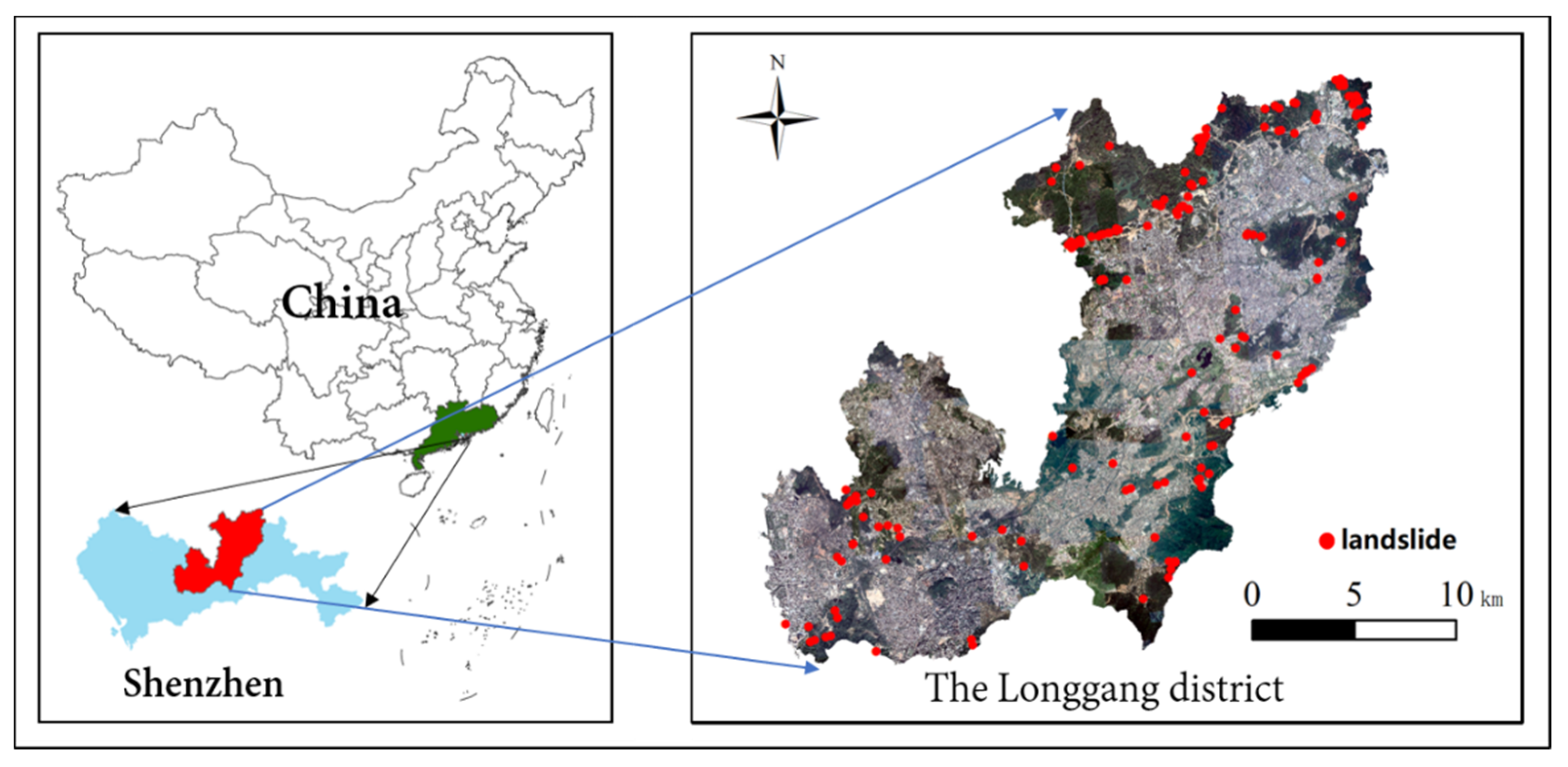
Figure 1. The location of the study area in Longgang District, Shenzhen, Guangdong Province, China. The red points are the locations of identified landslides in the detailed survey of 1:50,000 geological disasters in Longgang District, Shenzhen.
Remotesensing 13 03383 g001
Figure 2. The fault zone of Longgang District.
Remotesensing 13 03383 g002
Figure 3. Photographs showing the landslide in the Longgang study area. (a,b) Examples of landslides; (c) landslide beside the road; (d) landslide behind a house.
Remotesensing 13 03383 g003
Figure 4. The remote sensing images of different datasets. (a) The landslides remote sensing images of Longgang District. (b) The non-landslide remote sensing images of Longgang District. (c) The landslide images of Bijie City. (d) The non-landslide images of Bijie City. (e) The images of the UC Merced land use dataset. (f) Yhe images of the WHU-RS19 dataset. (g) The images of the SIRI-WHU dataset. (h) The images of the NWPU-RESISC45 dataset.
Remotesensing 13 03383 g004
Figure 5. The structure of the DDTL.
Remotesensing 13 03383 g005
Figure 6. The image processing with autoencoder.
Remotesensing 13 03383 g006
Figure 7. The structure of improved attention module based on CBAM.
Remotesensing 13 03383 g007
Figure 8. The framework of the proposed AM-DDTL model.
Remotesensing 13 03383 g008
Figure 9. The original high-resolution images from Google Earth and the enhanced images. (a,c) The Longgang landslide high-resolution images. (b,d) The enhanced images after image enhancement.
Remotesensing 13 03383 g009
Figure 10. The framework of CNN and pretrained model.
Remotesensing 13 03383 g010
Figure 11. The comparison of DDTL, SE-DDTL, CBAM-DDTL and improved CBAM. (a) The source domain is the Bijie landslide dataset. (b) The source domain is the UC Merced land use dataset. In the subfigure, upper left is total loss, upper right is reconstruction loss, lower left is classification loss, and lower right is domain loss.
Remotesensing 13 03383 g011
Figure 12. The different effects of different kernel sizes.
Remotesensing 13 03383 g012
Figure 13. The feature map of different attention mechanisms based on DDTL. (a) The original landslide remote sensing images. (b) The feature map of DDTL without attention mechanism. (c) The feature map of SE-DDTL model. (d) The feature map of CBAM-DDTL model. (e) The feature map of improved CBAM-DDTL model.
Remotesensing 13 03383 g013
Figure 14. The comparison of different source domains.
Remotesensing 13 03383 g014
Figure 15. The domain loss of different source domains.
Remotesensing 13 03383 g015
Figure 16. The experimental outcomes of different source domain combinations; for the multisource domain, the Bijie landslide dataset is the primary source domain, and the other remote sensing images are the auxiliary source domain. (a) The auxiliary source domain is WHU-RS19. (b) The auxiliary source domain is SIRI-WHU. (c) The auxiliary source domain is the UC Merced land use dataset. (d) The auxiliary source domain is NWPU-RESISC45.
Remotesensing 13 03383 g016
Table 1. The source domains in this paper.
DatasetImagesTotal Images
Bijie landslide dataset770 landslides samples and 2003 negative samples2773
UC Merced land use dataset21 classes × 100 images2100
Google image dataset of SIRI-WHU12 classes × 200 images 2400
WHU-RS1912 classes × 50 samples1005
NWPU-RESISC4545 classes × 700 images31,500
Table 2. The results of different models using enhanced images and original images.
Enhanced ImagesOriginal Images
AccuracyPrecisionLossAccuracyPrecisionLoss
CNN86.160.89740.914483.940.89150.5518
VGG-1687.090.86740.867485.710.85040.3503
VGG-1988.240.90850.214486.260.88350.2572
ResNet-5089.860.91300.829988.380.90851.0596
DDTL88.010.91740.734287.940.91140.8465
Table 3. The total loss of different data.
Target domainRGBDEMRGB + DEM
Source domainRGBDEMRGB + DEM
Total loss19.63627.8417.65
Table 4. The accuracy of different attention mechanisms based on DDTL.
DatasetDDTLSE-DDTLCBAM-DDTLImproved DDTL
Bijie landslide dataset79.6993.3695.8996.03
UC Merced land use dataset87.3394.5795.7896.78
Table 5. The accuracy of different source domains.
Auxiliary Source DomainRS19-WHUSIRI-WHUUC Merced Land UseNWPU-RESISC45
Primary Source DomainThe Bijie landslide dataset
Single source87.9693.6392.3896.01
Multisource94.0396.2594.4696.53
Publisher’s Note: MDPI stays neutral with regard to jurisdictional claims in published maps and institutional affiliations.