Article

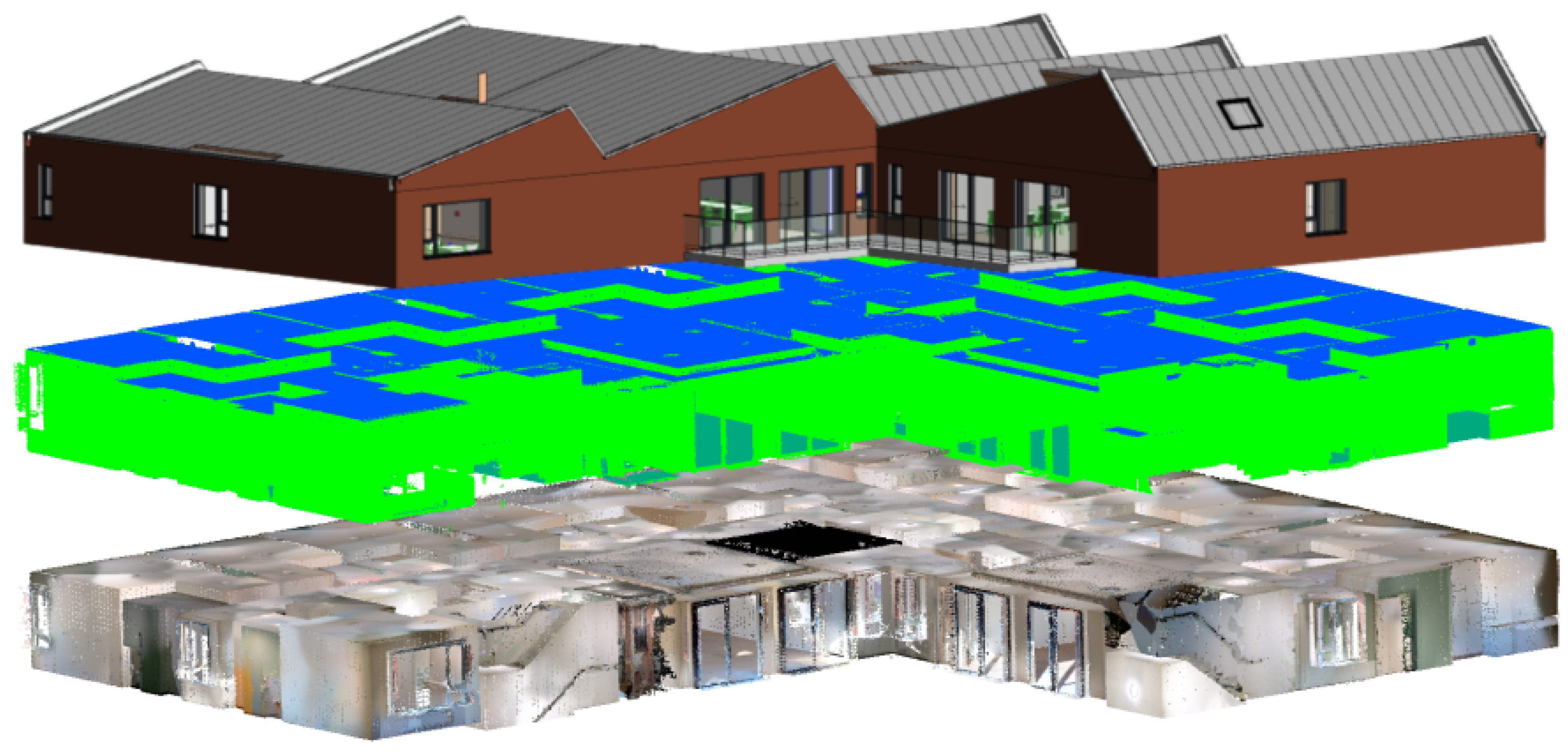
Point Cloud Validation: On the Impact of Laser Scanning Technologies on the Semantic Segmentation for BIM Modeling and Evaluation

by
Sam De Geyter
1,2,†,
Jelle Vermandere
1,†,
Heinder De Winter
1,†,
Maarten Bassier
1,*,† and
Maarten Vergauwen
1,†
1
KU Leuven Geomatics Research Group, Department of Civil Engineering, Technology Cluster Construction, Faculty of Engineering Technology, 9000 Ghent, Belgium
2
MEET HET BV, 9030 Ghent, Belgium
*
Author to whom correspondence should be addressed.
All authors contributed equally to this work.
Remote Sens. 2022, 14(3), 582; https://doi.org/10.3390/rs14030582
Submission received: 29 November 2021 / Revised: 12 January 2022 / Accepted: 19 January 2022 / Published: 26 January 2022

Abstract

:
Building Information models created from laser scanning inputs are becoming increasingly commonplace, but the automation of the modeling and evaluation is still a subject of ongoing research. Current advancements mainly target the data interpretation steps, i.e., the instance and semantic segmentation by developing advanced deep learning models. However, these steps are highly influenced by the characteristics of the laser scanning technologies themselves, which also impact the reconstruction/evaluation potential. In this work, the impact of different data acquisition techniques and technologies on these procedures is studied. More specifically, we quantify the capacity of static, trolley, backpack, and head-worn mapping solutions and their semantic segmentation results such as for BIM modeling and analyses procedures. For the analysis, international standards and specifications are used wherever possible. From the experiments, the suitability of each platform is established, along with the pros and cons of each system. Overall, this work provides a much needed update on point cloud validation that is needed to further fuel BIM automation.

Graphical Abstract

1. Introduction

The demand of Building Information Modeling (BIM) databases of existing buildings is rapidly increasing as the BIM adaption in the construction industry is expanding [1]. BIM models are requested for early design stages for refurbishment or demolition [2], as-is models are requested for facility management and digital twinning [3], as-built models are requested for project delivery and quality control, and so on [4]. This fast growing industry relies on surveyors and modelers to produce accurate and reliable Building Information Modeling objects as well as evaluate already modeled objects with the as-built situation.
For these procedures to be successful, it is important that all the components needed to model/evaluate the structure can be extracted. To this end, Lidar-based point cloud data is captured of the existing structure. This point cloud data is then interpreted by experts or automated procedures that model and evaluate all the visible BIM objects that are part of the scope. As such, proper point cloud data is the key to successful BIM processes and any defects to this input will have severe consequences for the quality, completeness, and reliability of the final model/evaluation [5].
Currently, BIM modeling/evaluation methods limit their scope to idealized data and assume that the semantic and instance segmentation have operated perfectly. However, this is very much not the case as sensor specifications, temporal variations, object reflectivity characteristics and so on have a massive impact on the resulting point cloud, which in turn affect the segmentation process. In this research, we will therefore study the discrepancies between point cloud inputs and evaluate their processing results at key stages (Figure 1). Concretely, we will evaluate the impact of different types of point cloud data on the semantic segmentation step. Additionally, we will analyze which modeling/evaluation information can be reliably extracted from the various point clouds. In summary, the works main contributions are:
1.
A detailed literature study on point cloud processing from the static and mobile Lidar data acquisition to the semantic segmentation;
2.
A capacity study of four state-of-the-art static and Lidar mobile mapping solutions;
3.
An empirical study of the impact on the semantic segmentation step based on international specifications;
4.
An in-depth overview of the BIM information that can be reliably extracted from each system for modeling/evaluation.
The remainder of this work is structured as follows. The background and related work is presented in Section 2. In Section 3, the sensors used in this study are presented. Following is the methodology for the capacity and semantic segmentation suitability study in Section 4. In Section 5, the test sites are introduced, along with their corresponding results in Section 6. The test results are discussed in Section 7. Finally, the conclusions are presented in Section 8.

2. Background and Related Work

In this section, the related work for the key aspects of this research are discussed: (1) the suitability of prominent indoor photogrammetric and Lidar data acquisition approaches for as-built modeling and analyses, (2) an overview of the data impact on semantic segmentation processes, (3) the inputs for scan-to-BIM methods and (4) validation methods and specifications.

2.1. Data Acquisition

Photogrammetry and Lidar-based geometry production are the most common in BIM modeling/evaluation procedures. Terrestrial, oblique, and aerial photogrammetry are among the most versatile measurement techniques. These systems are low-cost, can be mounted on nearly any platform and produce high-quality and dense texture information at an unparalleled rate. However, extensive processing of the imagery is required to produce suitable point clouds or polygon meshes. While current software such as Agisoft Metashape [6], Pix4Dmapper [7], and RealityCapture [8] are capable of matching thousands of unordered images in a matter of minutes, the subsequent dense point/mesh reconstruction can take several days for large-scale projects without guaranteed success. Furthermore, photogrammetric routines can underperform in indoor environments due to extreme lighting variations and low-texture variance on smooth objects. Drift and scaling also remain troublesome bottlenecks for photogrammetry-based routines and thus require the use of labor-intensive control networks to achieve suitable accuracy [9].
Alternatively, static and mobile Lidar-based systems have a higher applicability as they can operate in poorly lit environments due to their active remote sensing. These systems also directly produce the highly accurate point cloud data without the need for extensive post-processing. Static Terrestrial Laser Scanners (TLS) are currently the most popular systems for any type of building documentation. These systems generate millimeter range errors and accumulate little to no drift throughout consecutive scans due to the high quality of the data [10]. High-end TLS are among the few systems that can effectively operate without the need for control networks, which reduces the time on site by an average of 39% [10]. However, significant post-processing time can halt these systems as the registration of the consecutive scans still requires significant human interaction.
On the other hand, Indoor Mobile Mapping systems (iMMs) benefit from continuous data acquisition which greatly improves the coverage while also lowering the data acquisition time [11]. The post-processing is also significantly less labor-intensive, as the registration is tied to the sensor localization which is mostly performed unsupervised. Most iMMs leverage both Lidar and photogrammetric techniques to ensure robust localization of the system [12]. However, iMMs can generate significant drift in low-texture or low geometric variance areas and thus still rely on control networks to maintain accuracy [13]. Several researchers have compared both low-end and high-end iMMs including Matterport, SLAMMER, NavVis, and Pegasus [14,15]. Depending on the Simultaneous Localization and Mapping (SLAM) algorithms for the localization, high-end systems in 2021 can maintain 20 mm accurate tracking for small-scale projects [14,16]. Overall, TLS is still the most popular technique due to its robustness and accuracy, but iMMs are rapidly closing the gap with their faster data acquisition and increasingly more accurate localization [17].

2.2. Data Processing

Data processing steps aim to process initial geometric data so BIM objects can be modeled/evaluated based on the points as unsupervised as possible. Prominent steps include data structuration, primitive segmentation, and semantic and instance segmentation. The key step is the semantic and instance segmentation that assigns class labels to a subset of geometric inputs e.g. the assignment of a column class to a section of the point cloud. This step is very impactful, but there is currently a gap in the literature regarding how different geometry inputs affect the semantic and instance segmentation.
Deep learning currently is by far the most popular method to conduct semantic segmentation and instance segmentation. A plethora of Convolutional Neural Network (CNN) architectures have spawned that are fueled by increasingly larger datasets such as ScanNet, Rio, S3DIS [18], SEMANTIC3D [19], ISPRS, etc., [20]. Several of these networks are Open-Source which are continuously innovated and can easily be adapted for other tasks. However, the inputs generally are fixed. The dominant geometry inputs are 2D rasters from structured data sensors, 3D voxels structured in octrees or kd-trees that can be generated from any point cloud, the raw point cloud, and finally also polygonal meshes [21].
Popular 2D rasterized multiview CNN (MVCNN) are SnapNet [22], MVDepthNet [23], and 3DMV [24]. These methods closely align with image semantic segmentation networks and thus can benefit from their advancements. However, through the reduction to 2D rasters from the sensor’s vantage point, a significant portion of geometric features is ignored, e.g., the coplanarity of opposite wall faces. Similarly, rasterized 2D slices from 3D point clouds only allow for a partial interpretation of the scene with limited features [25]. This downside is compensated with an unparalleled speed, with MVCNNs performing near real-time [26].
Popular voxel-based networks are VoxNet [27], SegCloud [28], OctNet [29], O-CNN [30], and VV-NET [31]. These approaches are known for their speed and holistic features. However, voxel-based methods reduce the spatial resolution and thus can underform near edges and details.
Popular point-based networks are PointNet [32], PointNet++ [33], PointCNN [34], PointSIFT [26], SAN [35], and RandLA-Net [36]. These network compute individual point features in addition to conventional global features, leading to a performant semantic segmentation without a reduction in spatial resolution. As point-based classification best reflects the impact of input variations, these methods are ideally suited for the input validation. Of specific interest is RandLA-Net, which is one of the most performant recent networks that was also trained on the Stanford 2D–3D-Semantics Dataset (S3DIS), which closely aligns to typical indoor environments.
Polygonal meshes will be a serious contender with point cloud methods as they significantly reduce the data size (up to 99% reduction) while preserving geometric detailing. However, the work on polygonal meshes is still very much a subject of ongoing research and thus is not yet as performant as the above methods [37].

2.3. Reconstruction Methods and Inputs

Once the inputs are processed to a set of observations that each represent a single object instance, the data are fed to class-specific reconstruction algorithms that attempt to retrieve the object’s class definition and parameter values. Reconstruction algorithms vary wildly depending on the class of the object (walls vs. ceilings or doors) and even within a single class there are a plethora of methods such as those discussed in our previous work [38]. A key difference between methods is the type of object geometry that is pursued. For instance, there are the boundary-based representations such as in CityGML that solely model the exterior of an object, typically in an explicit manner such as with polygonal meshes. In contrast, volumetric object representations such as in BIM require knowledge about the internal buildup of an object and are more frequently modelled in an implicit manner, i.e., based on parametric design. For a typical class such as walls, this difference is very pronounced. Boundary-based walls will have their wall faces reconstructed individually and are solely linked through semantics. This makes it very easy for both 2D and 3D reconstruction methods that have to fit the best fitting surface on each visible surface of the wall and correctly draw the niches, protrusions, and openings in that surface [39]. In contrast, volumetric walls will be reconstructed by accurately estimating the wall object parameters such as the hearth line, the height and the thickness along with additional parameters for each opening, niche, and protrusion that each also have their parameters [40]. The semantic segmentation plays a vital role in whether a reconstruction method will achieve success as it lies at the basis of the geometry assumptions of a class. For instance, the assignment of a column class to a section of the point cloud decides that a parameter extraction algorithm or a modeler will fit a column to that section, regardless of whether that is correct. If part of that column is mislabeled, it is very likely to upset any parameter estimation of the final object’s geometry. Finally, the topology between objects will also be severely distorted by rogue objects that are being created because of misclassifications [41]. Any interpretation error therefore directly and exponentially propagates the error in the reconstruction and the typology configuration step and must be avoided.

2.4. Validation Methods and Specifications
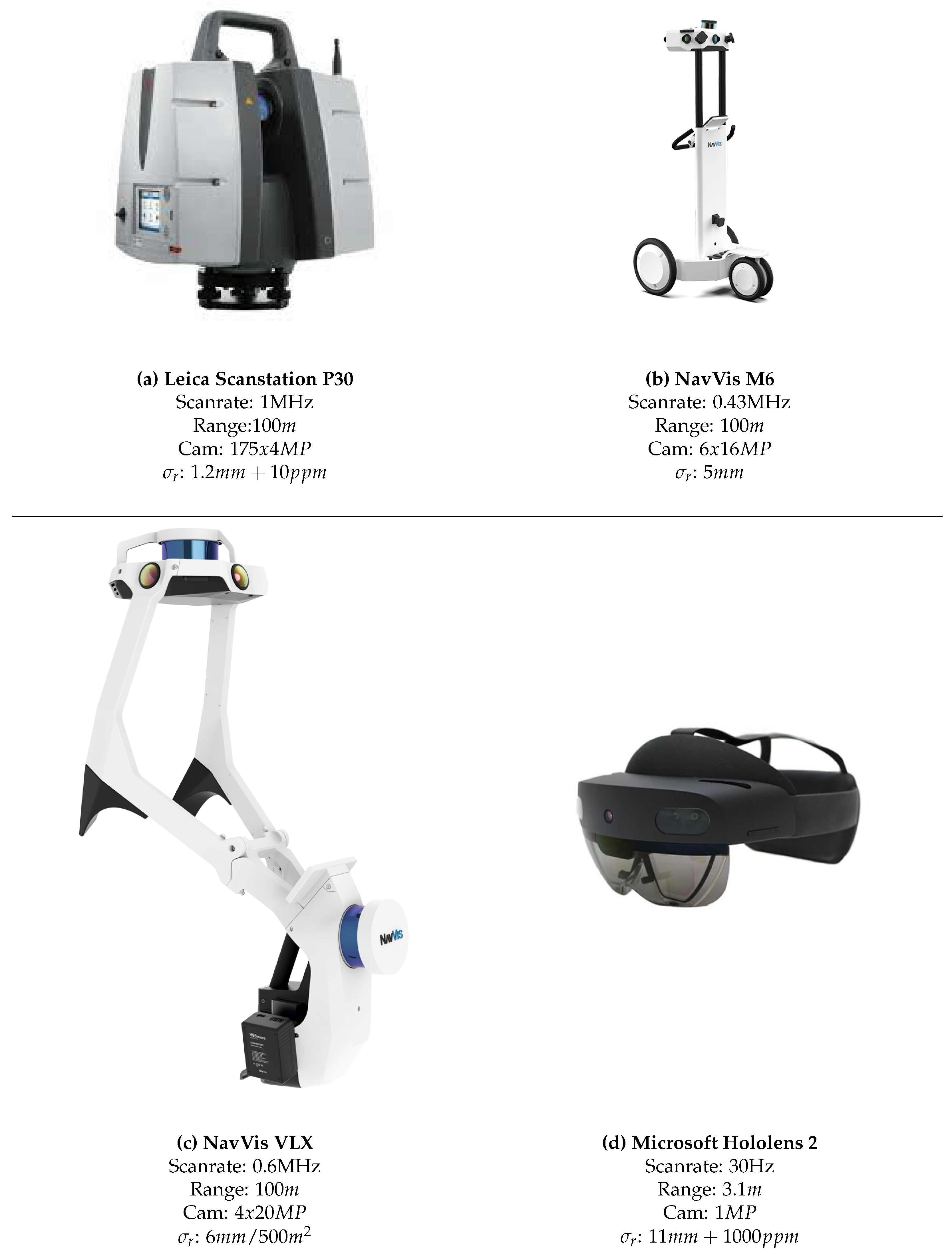
Concerning the impact of data acquisition on the data processing, few comparisons are currently available. However, there are several researchers that formulate validation criteria for the point cloud and the semantic segmentation with relation to BIM.
For the point cloud validation, most researchers only perform an accuracy analysis on the point cloud data [13,16,17]. The closest related works for a more holistic validation are those of Rebolj et al. [42] and Wang et al. [4], in which the quality criteria of point cloud data for Scan-to-BIM and Scan-vs.-BIM are established which we translate to LOA and LOD definitions in Table 1 and requirements in Table 2. Aside from the accuracy, they determine parameters for the completeness and density of the point cloud that are required to model various building elements. For the accuracy, researchers either report deviations on benchmark datasets directly, or refer to international specifications such as the Level of Accuracy (LOA) [43], the Level of Development (LOD) [44], or the Level of Detail [45] (Table 1). An interesting work is that of Bonduel et al. [46] who take into consideration the occlusions of the objects when computing the accuracy.
For the data processing, researchers typically report cross-validation or testing rates on the above benchmark datasets. Popular metrics include recall and precision, F1-scores and Intersection over Union (IoU) of the ground-truth data, and the prediction of the network. These metrics give a good overall overview of the network’s performance. For a more in-depth study, call-outs of specific objects are typically gathered and subjected to a visual inspection. In this work, both methods will be used to evaluate the impact of the data acquisition differences on the semantic segmentation.

3. Sensors

In this section, the sensors used for indoor mapping are presented. The specifications per sensor are discussed, as well their advantages and shortcomings. Concretely, we compare a high-end terrestrial laser scanner with two state-of-the-art iMMs and one low-end mapping sensor. For the experiments, the TLS data and a manually created as-built BIM model are taken as the baseline to compare the impact of the sensors on the data capture and processing.

3.1. Leica Scanstation P30

Static Terrestrial Laser Scanning (TLS) (Figure 2a) is the most conventional and accurate Lidar-based data acquisition solution on the market. Current direct and indirect Time-of-Flight sensors can capture full-done scams in only a couple of minutes with scanrates up to 1–2 MHz. Furthermore, the images takes by the sensor can now also be used in structure-from-motion pipelines to automatically register consecutive point clouds. The raw outcome for indoor environments typical is a structured point grid of 10 to 40 Mp, similar to a spherical depth map and with a transformation matrix for each setup. The typical single point accuracy is <5 mm/50 m which corresponds to LOA40 [43]. Additionally, less than 1 mm of error propagation can be expected throughout consecutive setups [47].

3.2. NavVis M6

Cart-based indoor Mobile Mapping systems (Figure 2b) are the most stable of the indoor mobile solutions. Theoretically, these are also the most accurate mobile solutions as they can pack more high-end (and heavier) Lidar sensors and only require 4 Degree-of-Freedom (DoF) SLAM in most cases. These iMMs’ Lidar sensors yield unordered point clouds with uneven point distributions and thus are ideally suited for voxel-based semantic segmentation, although other representations are also possible. Overall, iMMs point clouds are less dense than static scans but have better coverage and are captured up to three times faster [17]. The typical global accuracy in 2021 is <2 cm (LOA20–LOA30) along the trajectory of the system and local point accuracy is similar to TLS (LOA40). The stable localization is mainly due to the camera-based SLAM that, together with the Lidar and the motion sensor, provides a well-rounded tracking mechanism.

3.3. NavVis VLX

Backpack-based indoor Mobile Mapping systems (Figure 2c) are a more dynamic iMMs variant that still pack high-end Lidar sensors but have increased accessibility. Their random trajectory is typically tracked through 6 DoF SLAM, which theoretically is more error prone in low-texture or low geometric variance areas depending on localization sensors. However, 4 DoF SLAM is also affected for these zones, and thus iMMs performances are more tied to the environment and sensors than the concrete setup. As such, similar accuracies of LOA20–LOA30 for the global point accuracy and LOA40 for the local point accuracy are reported for these systems. Analogue to the M6, the combination of Lidar-and camera-based SLAM yields superior results. An important feature, however, is the software that ships with each system. With NavVis, the software inherently allows for the inclusion of ground control points in an automated manner which is not the case with low-end sensors. These control points are actively used during post-processing and function as fixed constraints in the bundle adjustment of the scan network.

3.4. Microsoft Hololens 2

A recent addition to capturing devices are Mixed Reality systems (Figure 2d). These portable data acquisition solutions can be considered iMMs but do not have the same large-scale mapping capabilities. They are part of this study’s scope, as these systems will play a major role in digital built environment interaction which inherently includes mapping. They operate with 6 DoF SLAM but can only be deployed for smaller scenes due to poor field-of-view, range, and low-end sensor specifications. Single-point accuracies of 1 cm/m for the Lidar sensors are not unusual with a high error propagation, restricting them to close-range applications (LOA10–LOA20). Specifically for the Hololens 2, the spacial mapping is designed to run as a background task, using minimal resources to keep the device performant. Being a head-mounted device, the mobility leaves no restrictions for the user. The capabilities are focused on real-time mapping and less on accuracy. This results in on-device-computed meshes that can be used directly in the processing. These are generally lower in resolution so they can be stored on the device, but are also usable for mapping. However, the restricted range of only circa 3–4 m is a significant downside for BIM modeling/evaluation.

4. Methodology

In this section, the methodology is formulated to determine the impact of data acquisition and the subsequent semantic segmentation on the point cloud suitability for BIM modeling/evaluation. Concretely, we first conduct a sensor capacity test, where each sensor is tested to produce proper point cloud data. Next, we evaluate the point cloud suitability for BIM modeling/evaluation in a detailed study where each system’s data is semantically segmented and evaluated whether the results can be used for as-built BIM modeling or analyses. We use international specifications such as the LOA [43] and common literature metrics wherever possible to provide a clear comparison of the results.

4.1. Sensor Capacity

First, a quantitative analysis on the point clouds is conducted to analyze the raw performance of each system (Figure 3). As is common in the literature, we evaluate the sensor accuracy and error propagation along the trajectory by computing the Euclidean cloud-to-cloud (c2c) distances between the sensor’s point cloud and the ground truth data. For these tests, the TLS data, which is confirmed to comply to LOA40 [2 σ < 0.005 m] by total station measurements, is considered as the ground truth. To compare the point clouds, all datasets are referenced to the same coordinate system and only the overlapping areas are evaluated. For every point cloud, the cumulative percentage of c2c-distances are computed at 68% and 95% inliers as reported by [48]. Furthermore, the metrics will be compared to the LOA specifications as stated in [43]. The overlapping point clouds are reported cumulatively for each bracket, i.e., LOA30 [2 σ < 0.015 m], LOA20 [2 σ < 0.05 m] and LOA10 which is user-defined and set to [2 σ < 0.1 m] conform common building tolerances [4].
To asses the capacity of each system, the need for loop closures and control points needed to obtain accurate results, are evaluated. This knowledge is vital to obtain a maximal efficiency on site with a minimal amount of time needed to capture a scene. These characteristics are tested by mapping the same datasets shown in Figure 3, with and without control points and loop closures. First, a long hallway is mapped without possibility for loop closures to test the raw tracking cabailities of each device. The narrow pathway and scene repetitiveness pose key challenges for iMMs and thus significant drift can be expected this subideal D-hall dataset (Figure 3a).
Analogue, the influence of loop closures, is measured by mapping the same loop with and without loop closures (Figure 3b). To this end, a square shaped corridor is mapped with the different systems. The P30 is again used as a reference and is validated with control points on each corner of the square. The passage between the starting and end point of the loop is important in this dataset. To ensure an unbiased evaluation, the passage was closed off so the raw drift of each system could be measured directly by observing both sides of the passage. When loop closures were to be applied, the passage was left open so the processing software could align the starting and end zone.

4.2. Point Cloud Suitability
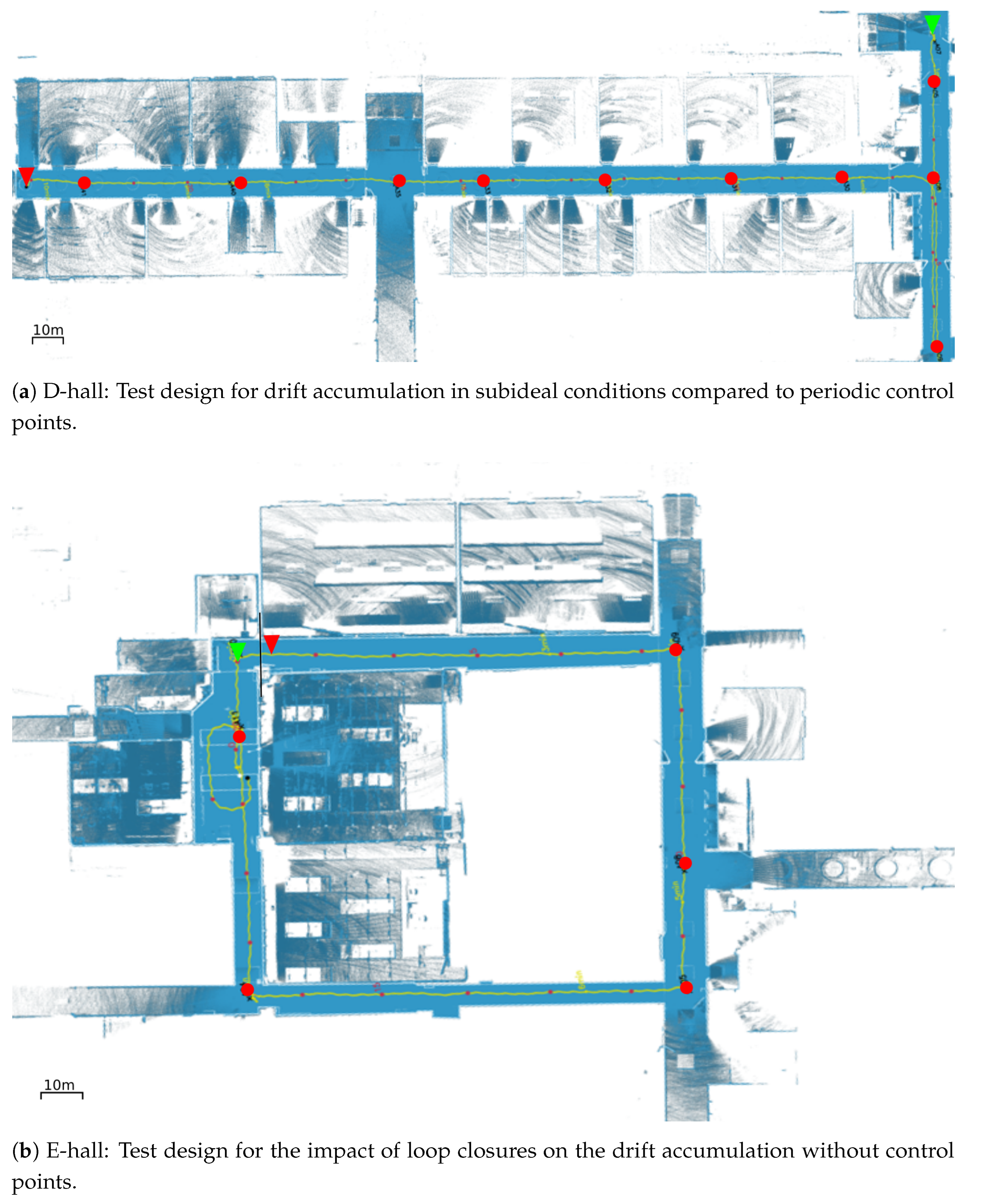
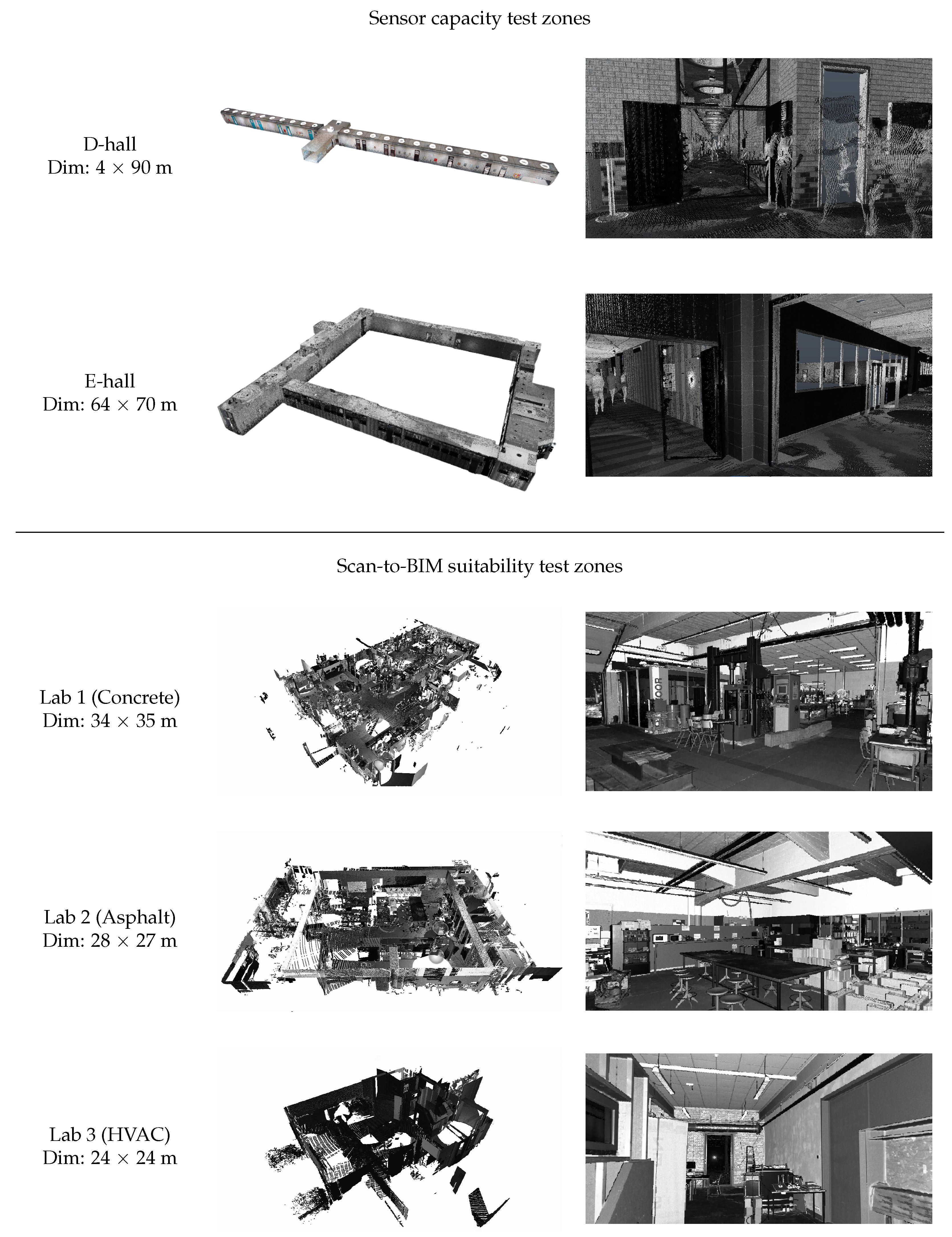
The second analysis evaluates each system’s capabilities for BIM modeling and evaluation. As described in the related work, the key stages that influence this process are the initial geometry production and the semantic segmentation. In this test, we evaluate both aspects for each system on 3 distinct target areas (see Section 5). We test 5 common structure classes that are part of most unsupervised BIM reconstruction/analyses methods as they form the observable core of each structure, i.e., ceilings, floors, walls, beams and columns. For these experiments, a manual as-built BIM is conceived as accurately as possible by expert modelers. Analogue to the capacity tests, the P30 data are used as the main repository as they is proven to comply with LOA40. However, in areas where the P30 did not capture any data, the Leica VLX was used in combination with control points and loop closure which is also highly accurate and has the best coverage.
From the literature, the BIM information extraction requirements for these classes are established. Table 2 depicts the expected Level of Accuracy and Level of Development that are commonly reported for the structure classes [2,3,49].
The point cloud suitability of the initial geometry production is established by translating the above requirements to point cloud parameters for quality, completeness and detailing as reported by Wang et al. [4] and Rebolj et al. [42]. We report each parameter per class, based on its semantic segmentation. As such, we can asses how well the different classes correspond to the expected requirements.
It is important to notice that significantly lower inliers are expected for the represented accuracy due to modeling abstractions. For instance, none of the sensors achieve LOA30 in any of the test cases as abstract BIM objects are used to represent the geometry (which is custom in industry), that do not take into consideration the detailing and imperfections of the real environment. Furthermore, while the filtering algorithm for the classes (see Methodology) achieves a proper segmentation, some noise and clutter can be expected that will negatively impact the number of inliers. However, we can still evaluate the relative performance between the sensors to establish the point cloud suitability.
The quality is established by the point accuracy similar to the capacity tests with the c2c-distance being evaluated. However, the LOA represented accuracy (point cloud vs. model) is evaluated rather than the documentation accuracy (point cloud vs. point cloud) in the above tests (Equation (1)). As such, the BIM is uniformly sampled ( P synth ) and used as the reference for each dataset’s distance evaluation, which also allows us to evaluate the suitability of the TLS. To ensure a balanced quality measure, we uniformly sample the input point clouds P up to 0.01 m, which does not compromise the number of LOA30 inliers. Similar to the above tests, the distance threshold t d is capped at 0.1 m to not include outlier points.
D = d | q Q , p P synth : min q p q < t d
As the point accuracy is not normally distributed, we report the inliers for the cumulative LOA30 [2 σ < 0.015 m], LOA20 [2 σ < 0.05 m] and LOA10 [2 σ < 0.1 m] brackets (Equation (2)).
Q u a l i t y = LOA 30 : | D < 0.015 m | | D | LOA 20 : | D < 0.05 m | | D | LOA 10 : | D < t d | | D |
The completeness of the point clouds is established by determining the coverage per class. Wang et al. [4] define this as the ratio between covered area and total area, but they correctly state that this is an ambiguous measure as it does not account for the clutter that occludes significant portions of the object. We therefore perform an initial filtering on P for each class based on t d . Additionally, we evaluate the normal similarity between the observed n ( q ) and the reference n ( p ) normals in both datasets [50] (Equation (3)).
Coverage = 1 | P synth | p P synth | q Q : argmin p p q < t d for which n ( p ) · n ( q ) > t
Finally, the density of each point cloud is established by the average spatial resolution of P. To this end, n samples are extracted from P for which the Euclidean distance to its nearest neighbor is computed (Equation (4)).
Density = 1 n i = 1 n d | p i , p j P : min p j p i p j
The subsequent semantic segmentation capacity is tested by processing each system’s dataset with the same state-of-the-art CNN. Concretely, we adapt RandLA-Net which was pretrained on Area 5 of the S3DIS stanford dataset [18]. The model was trained according to the specifics discussed in [36] and achieved on average 88% of the structure classes of S3DIS Areas 1–6 which are representative indoor scenes captured by a mobile RGBD scanner. From S3DIS, we solely retain the ceilings, floors, walls, beams, and columns classes and store the remainder in a clutter class, except, the classes windows, doors and boards, which are stored in the wall class, because these object classes are contained within the wall structure class and are modeled once the structure is completed.
As a baseline for the model expectations, we inherit the Hu et al. [36] mIoU values of each class given a 6-fold cross-validation (see Table 2). Additionally, we report the IoU values of an idealized synthetic point cloud of our datasets that are generated from the as-built model. Given the IoU values of each class, we will conduct a quantitative and visual analysis of the results.

5. Test Setups

The experiments are conducted in different areas of our university technology campus in Ghent, Belgium. In total, five test zones are developed for the sensor capacity and point cloud suitability tests (Figure 4).
For the sensor capacity test, two drift-sensitive areas are selected. The first is the D-hall (Figure 4, row 1) and the E-hall (Figure 4, row 2). Both hallways do not contain distinct features and form a monotonous scene. The D-hall trajectory (90 m) is specifically chosen to evaluate the drift of the different iMMs. The E-hall trajectory (120 m) is chosen to evaluate the effect of loop closure on each point cloud. In each zone, a control network was established with total station measurements and georeferenced in the Belgian Lambert 72 (L72) coordinate system. In the capacity tests, the Leica Scanstation P30 is used as the ground truth due to its superior accuracy which was established in previous work [46]. The alignment of the iMMs datasets with and without control points was performed with control points outside of the targeted survey area. Figure 3 shows the trajectory of M6 and the VLX, as well as the location of the control points. While the NavVis software allows a seamless integration with control and uses this in post-processing, this is not the case for the Hololens 2. Therefore, the Hololens 2 data were divided into chunks that were manually registered to the control. In Table 3, an overview of the survey is presented, including the time needed to map the zones and the manual intervention time in the post-processing that was required. The time for measuring end materializing the control points and time to prepare the sensors before data capture was not included as all methods employ this data.
For the point cloud suitability test, three industrial laboratories were selected. Lab 1 is used for concrete processing and contains hydraulic presses, aggregate storage, a classroom and several experiment setups (Figure 4, row 3). Lab 2 has facilities for road construction research including several environmental cabins and asphalt processing units (Figure 4, row 4). It also has several free standing desks, desktop computers, and a separate office space. Both these labs are located in a refurbished factory space where the concrete beams and columns are still visible. Finally, Lab 3 is a building physics lab in an adjacent masonry building which has visible steal beams and contains several experimental setups, i.e., a blowerdoor test, insulation setup and ventilation experiment (Figure 4, row 5). These environments are chosen for their representation of industrial environments and the presence of all target classes. The column class, however, is still underrepresented as the columns are located inside the walls, which will also negatively impact their coverage and subsequent semantic segmentation. However, the pretrained S3DIS model also suffers from similar issues as columns and beams are commonly occluded. Similar to the capacity test, each zone was mapped with the four sensors and georeferenced with TS measurements (Table 3). In this test, the synthetic point cloud generated from the as-built BIM is used as the ground truth for the quality, completeness, and semantic segmentation comparison.

6. Experimental Results

In this section, the results of the experiments to evaluate the sensor capacity and the point cloud suitability are discussed.

6.1. Sensor Capacity

6.1.1. Impact of Control Points

As discussed in Section 5, accumulative drift along the repetitive hallway is expected. Figure 5 reports the visual deviations and the inliers for each LOA bracket for the D-hall with and without the support of a control network. Figure 6a shows the percentual inliers with respect to t d = 0.1 m, conform common industry tolerances. Overall, the VLX and M6 iMMs maximum deviations fall within the threshold, showing less than 0.01 mm/10 m drift without control which is in line with the NavVis reports [51]. As expected, the low-end Hololens 2 reports much higher drift, with a maximum of 0.86 m deviation at 90 m. With the inclusion of control, the LOA30, 20, and 10 inliers for the M6 and the VLX, respectively, improve by 44.8% and 48.5%, while for the Hololens 2 this is only 21%. This is mainly caused by the poor close-range data quality of the Hololens 2, which prevents it from achieving LOA20 or 30 even without drift accumulation.
When compared to each other, the impact of the different sensors of each system on the drift can be observed. The experiments clearly show that the range errors of each system (Hololens 2: 0.01 m/1 m, M6: 0.01 m/10 m, and VLX: 0.01/50 m) play a major role in the drift accumulation. For low-end sensors, the close-range noise negatively impacts the data-driven SLAM which leads to increased drift. However, there is a clear drop-off of this affect when the range-noise drops below a certain point, i.e., the NavVis VLX Velodyne lidar sensors produce more qualitative data, and yet the drift accumulation is similar to the M6. This is due to the sideways configuration of the Lidar sensors, which thus only capture data that is less than 10 m away. As such, the distribution of the data and the quality of the motion sensor are more important in close-range scenes than further increasing the quality of the lidar sensor.
From the experiments, it can be concluded that without control, the M6 and VLX can be used small-scale projects up to LOA10 [2 σ < 0.10 m] and that the Hololens 2 is unsuitable for BIM modeling/analyses with these settings. With control, the M6 and VLX easily achieve LOA20 [2 σ < 0.05 m] close to LOA30 [2 σ < 0.015 m] when control is added circa every 25 m. Analogue, the Hololens 2 can achieve LOA10 close to LOA20 when control is added every 10 m. However, as discussed in Section 5, the Hololens 2 processing software does not yet have a functionality to import control points, and thus no control can be used during the adjustment of the Hololens 2 setups during processing. This is highly advised as control is one of the most effective ways to reduce drift accumulation for iMMs.

6.1.2. Impact of Loop Closure

The results of the loop closure experiments are shown in Figure 6b and Figure 7. Analogue to the control point evaluation, the accumulative error within the loop as well as the inliers for the consecutive LOA brackets are reported. First of all, all values are lower than in the E-hall. This is expected as the path is significantly longer (160 m opposed to 120 m) than in D-hall. As a result, maximum deviation of each system is 0.06 m for the M6, 0.2 m for the VLX, and 0.85 m for the Hololens 2. Upon closer inspection, this error is both in the X, Y, and Z directions which can be explained by the similar point distributions in these directions for E-hall. In terms of drift patterns, Figure 7 shows that the VLX slightly underperforms compared to the D-hall due to the increased length of the trajectory. Additionally, as the registration of the system has 6 DoF instead of 4 (see Section 3.3), an increased error can be expected from the randomized trajectory of the sensor. Similarly, the M6 loop closure optimization does not improve the results as the 120 m loop is too large for loop closure to compensate and thus fails to create a meaningful difference between the LOA20 and 30 inliers. This effect is more expressed for the Hololens 2, where the optimization of already properly aligned areas further improves, but poorly aligned areas do not shift towards a more accurate solution.
From D-hall and E-hall combined, the following conclusions are presented. In terms of control points, it is stated that the high-end iMMs can achieve LOA20 for circa 50 m of trajectory without the support of control points or loop closures. The low-end sensor can solely achieve LOA10 close to LOA20 when control is added every 10 m. In terms of loop closures, it is stated that the high-end iMMs can achieve LOA20 for circa 100 m of trajectory without the support of loop closures. The low-end sensor can solely achieve LOA10 close to LOA20 when loops are made every 30–40 m. While simultaneously applying control and loop closures does not significantly improve the result, there is a massive gain by using both techniques complementary. For instance, control networks only need to be established along the main trajectory of a building, while any short side-trajectories, (e.g., separate rooms) can be accurately mapped solely using loop closures.

6.2. Point Cloud Suitability

The quantitative results of the point cloud suitability experiments are shown in Table 4, Table 5 and Table 6. Each table includes the data acquisition parameters to evaluate the quality, completeness, and detailing as described in Section 4. The IoU percentages for the semantic segmentation of RandLA-Net are also reported per class and an overview of each classification is shown in the tables. Aside from the quantitative results, Figure 8, Figure 9, Figure 10, Figure 11, Figure 12 and Figure 13 show detailed call-outs to evaluate the point cloud’s suitability to be processed to individual objects. Each aspect is discussed below.

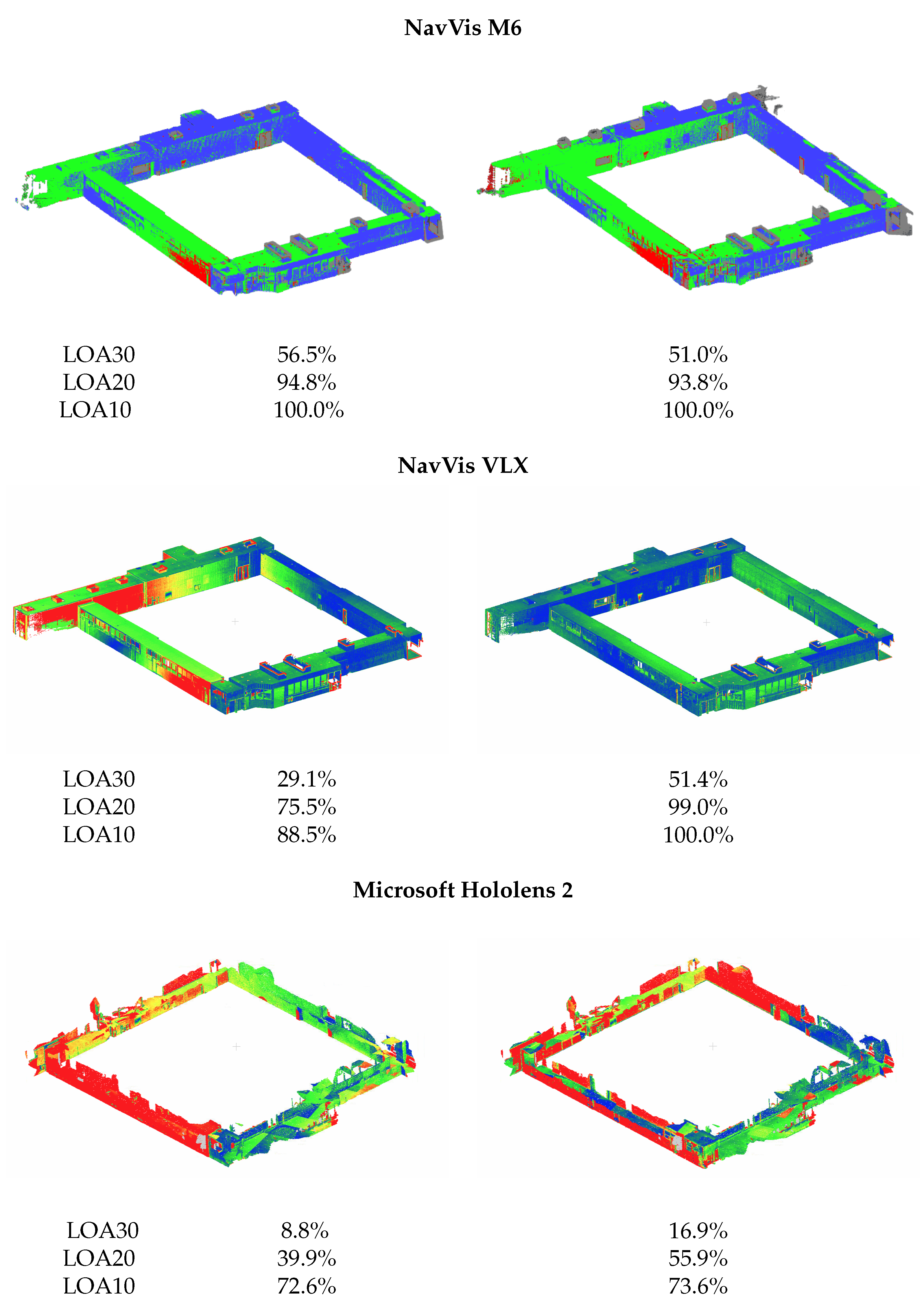
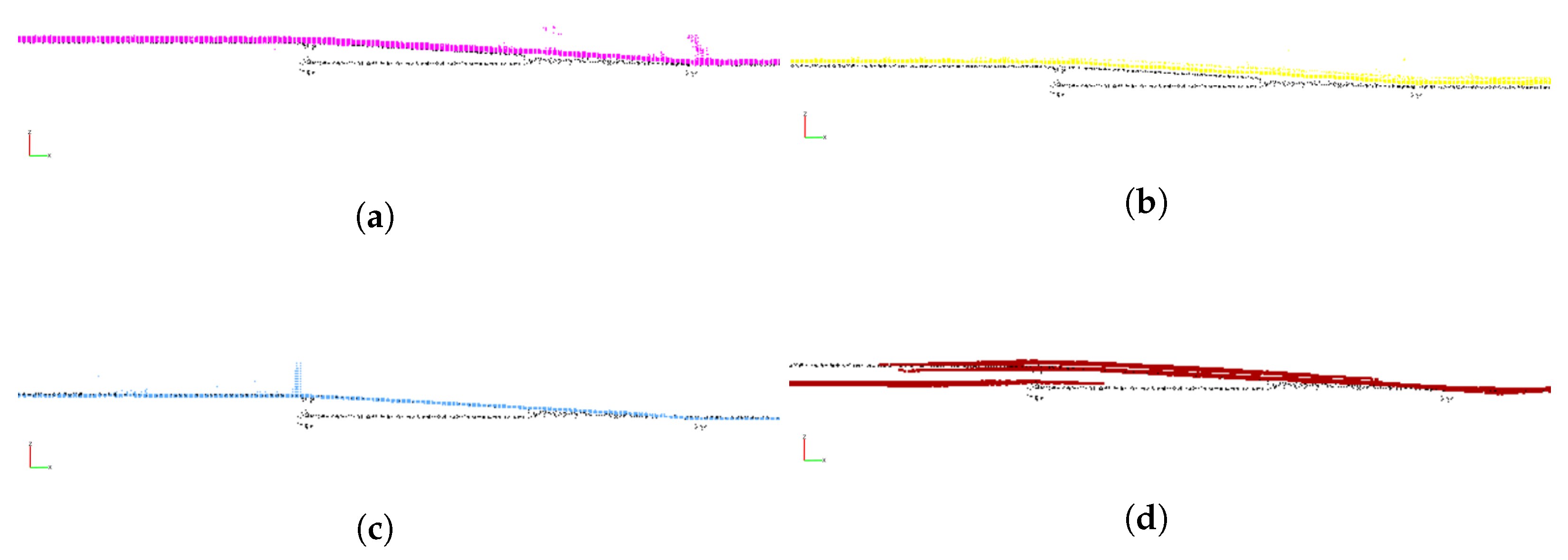
6.2.1. Impact of Quality

The accuracy of the captured data is reported as the LOA30, 20, and 10 inliers of the represented accuracy as discussed in the methodology. For the evaluation, it is important to notice that significantly lower inliers are expected for the represented accuracy due to modeling abstractions. For instance, none of the sensors achieve LOA30 in any of the test cases as abstract BIM objects, (i.e., IfcWallStandardCase) are used to represent the geometry as is custom in the industry. Furthermore, while the filtering algorithm for the classes (see Methodology) achieves a proper segmentation, some noise and clutter can be expected that will negatively impact the number of inliers. However, this dataset is the preferred reference to evaluate the relative performance between the sensors to establish the point cloud suitability.
Overall, from each sensor, LOA20 results (avg. 88%) could be reliably produced given the abstractions and clutter save for the Hololens 2, that on average has 10% less inliers. For objects that fit well with the abstract object definitions, the a BIM reconstruction from these point clouds will achieve LOA30 for the high-end sensors and LOA20 for the Hololens 2. Locally, this can improve to LOA40 for the high-end sensors and LOA30 for the Hololens 2. However, there are significant differences between each class. For instance, the average accuracies for the walls is significantly lower than for other classes. This is due to the increased abstractions. For instance, Lab 3 consists of ornamented masonry walls, leading to circa 35% lower inliers for the represented accuracy. For the ceilings, all iMMs surprisingly yield similar inliers, while this is not the case for the floors. Aside from abstractions, this is due to the sensor’s range noise, that misaligned the floor and the ceiling. When looking at the joint inliers, this is confirmed with the M6 (1 cm/10 m) and Hololens 2 (1 cm/m) on average showing 20% and 30% less inliers. Furthermore, when examined in more detail, a major error is detected in the floor data of the Hololens 2 (Figure 8). Due to its horizontality assumption, it does not properly detect the 0.1 m height difference in adjacent spaces in Lab 1. For the columns, the statistics show that each sensor achieves good LOA20 and even LOA30 results which is due to the positioning of these elements. Especially on square or rectangular elements, the number of inliers is very high. For the beams, the Hololens 2 again underperforms due to the height of the beams. However, specifically for beams and columns, statistics alone are very ambiguous as high Euclidean distance inliers do not guaranty proper point cloud processing. For instance, the increased noise on a beam section would make detailed modeling from the M6 data challenging and impossible from the Hololens 2.

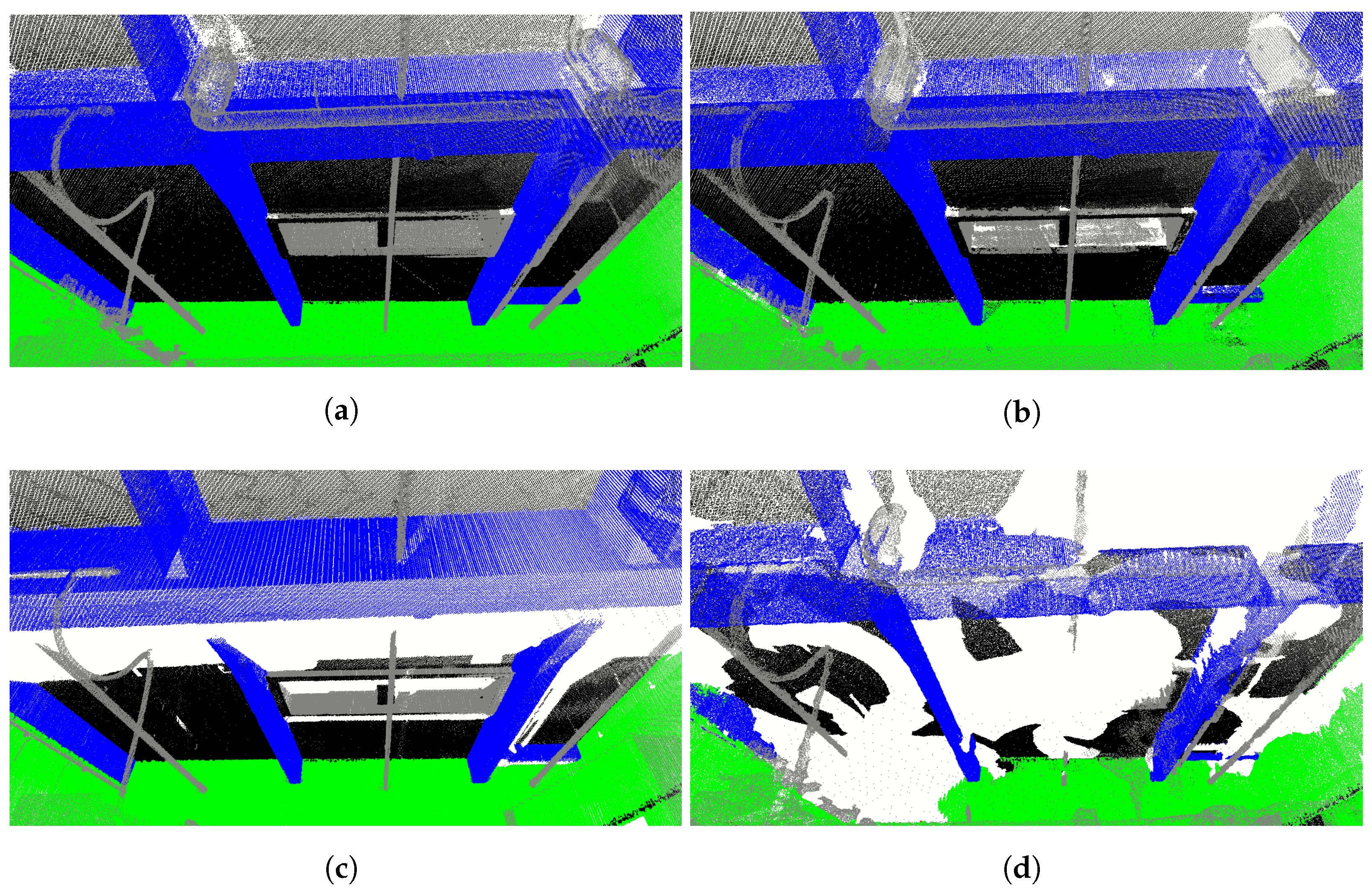
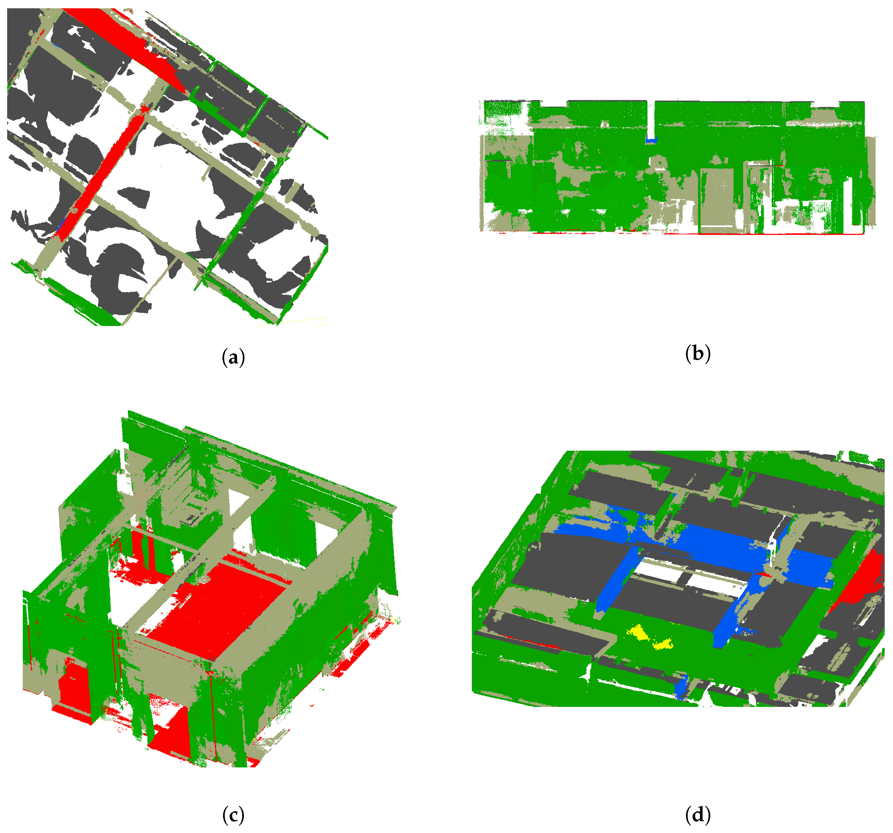
6.2.2. Impact of Completeness

In addition to the quality, the completeness is essential to create as-built models. Some occlusions are inevitable, i.e., with ceilings and floors, and this also reflects in the BIM LOD requirements that are lower for these categories.
The sensors achieved the following results. Overall, the VLX (60%) scores extremely high given the clutter and systematic occlusions, followed by M6 (52%), the P30 (41%), and the Hololens 2 (37%). This is due to the increased accessibility of the iMMs, where the backpack system scores circa 10% better than the cart-based system. Surprisingly, the highly mobile Hololens 2 underperforms, mainly due to its range limitations. This especially affects the capture of industrial sites where ceiling heights typically are more than 3–4 m. For higher and complex walls, the range of the Hololens 2 is insufficient, resulting in large parts of walls that remain unrecorded as can be seen in Figure 9. In contrast, the P30 underperforms due to its limited setups which leads to large gaping occlusions despite its range, e.g., Figure 10 shows that with the P30, massive occlusions exist on the ceiling when a beam is attached near the ceiling.
Overall, the coverage of floors with any sensor is much lower (on average <30%). The accessibility to the different floor parts is the driving factor for a proper point cloud. Especially in densely occupied spaces, every sensor struggles to achieve sufficient coverage to model anything more complex than a simplistic floor. However, the distribution of the occlusions varies widely between the sensors. The M6 and the P30, in particular, have large occlusions as they have restricted accessibility. With the other devices, however, it is possible to walk between obstacles (Figure 11). For the walls, the P30 and the Hololens 2 score on average 25% lower than the two other iMMs. However, their occlusions are very different with the P30 mainly struggling with clutter and the Hololens 2 missing large portions of the upper part of the walls due to its limited range. It is argued that the Hololens 2 occlusions are less impactful as these occlusions do not interfere with the proper modeling of the walls.
Analogue to the quality estimation, the coverage statistics for beams and columns are ambiguous as the impact drastically varies with respect to the beam/column type and the location of the occlusions. For instance, an I-profile, for which the section is partially occluded, prohibits proper modeling. For the exposed beams, the high-end sensors have an average coverage of 89%, while the Hololens 2 only achieves 58%. Furthermore, due to the height of the beams, a large portion of the section is occluded for the Hololens 2. For the largely occluded columns, all sensors achieve similar coverage as with the walls.

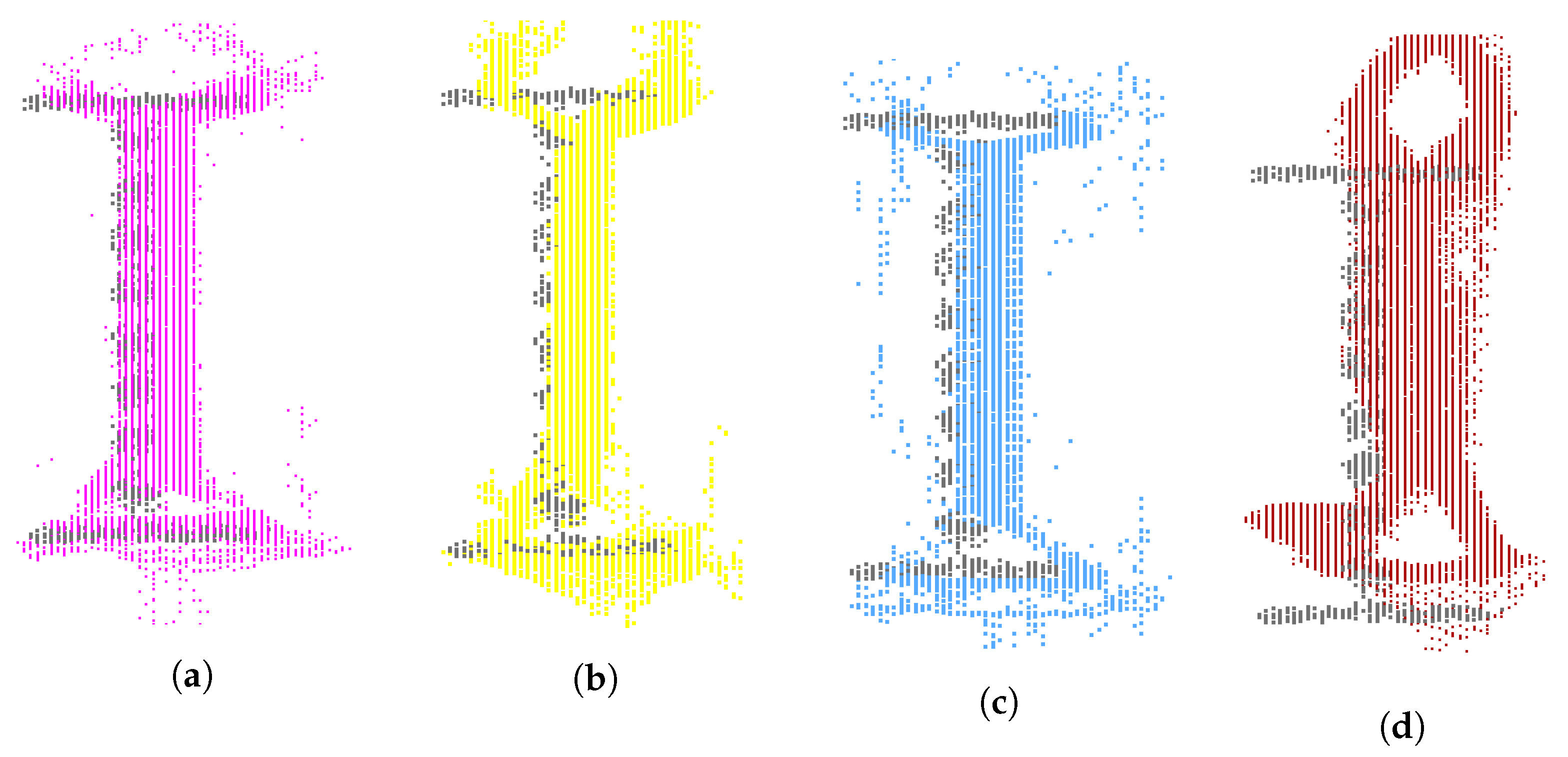
6.2.3. Impact of Detailing

The impact of the detailing of the point clouds varies wildly depending on the class and the complexity of the objects. For generic walls, ceilings and floor, even an extremely sparse point cloud suffices to properly model or analyze a LOD350 as-built BIM. In these cases, it is argued that the density of the P30, NavVis M6, and the NavVis VLX are complete overkill if their registration algorithms were not also data-driven. For the beams and columns, the opposite is true, e.g., for a modeler/algorithm to determine the proper beamtype, the resolution should be less than the flange thickness. For the high-end sensors, the density surpasses the flange thicknesses of most beam/column types so it is stated that LOD350 can be achieved with these sensors. The Hololens 2 data on the other hand does not allow the recognition of the proper beamtype as can be seen in Figure 13. Therefore, the Hololens 2 can only be used for object classes with details larger than 5 cm. With the high-end scanners, the detailing and resolution is sufficient, on the other hand with the Hololens 2, it must be possible to go close enough to the object in order to achieve good detailing.

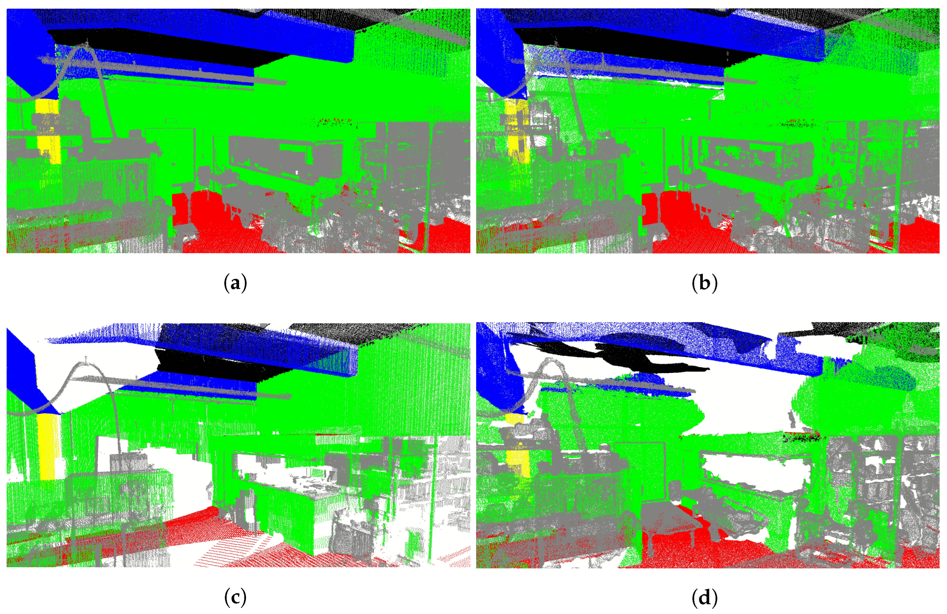
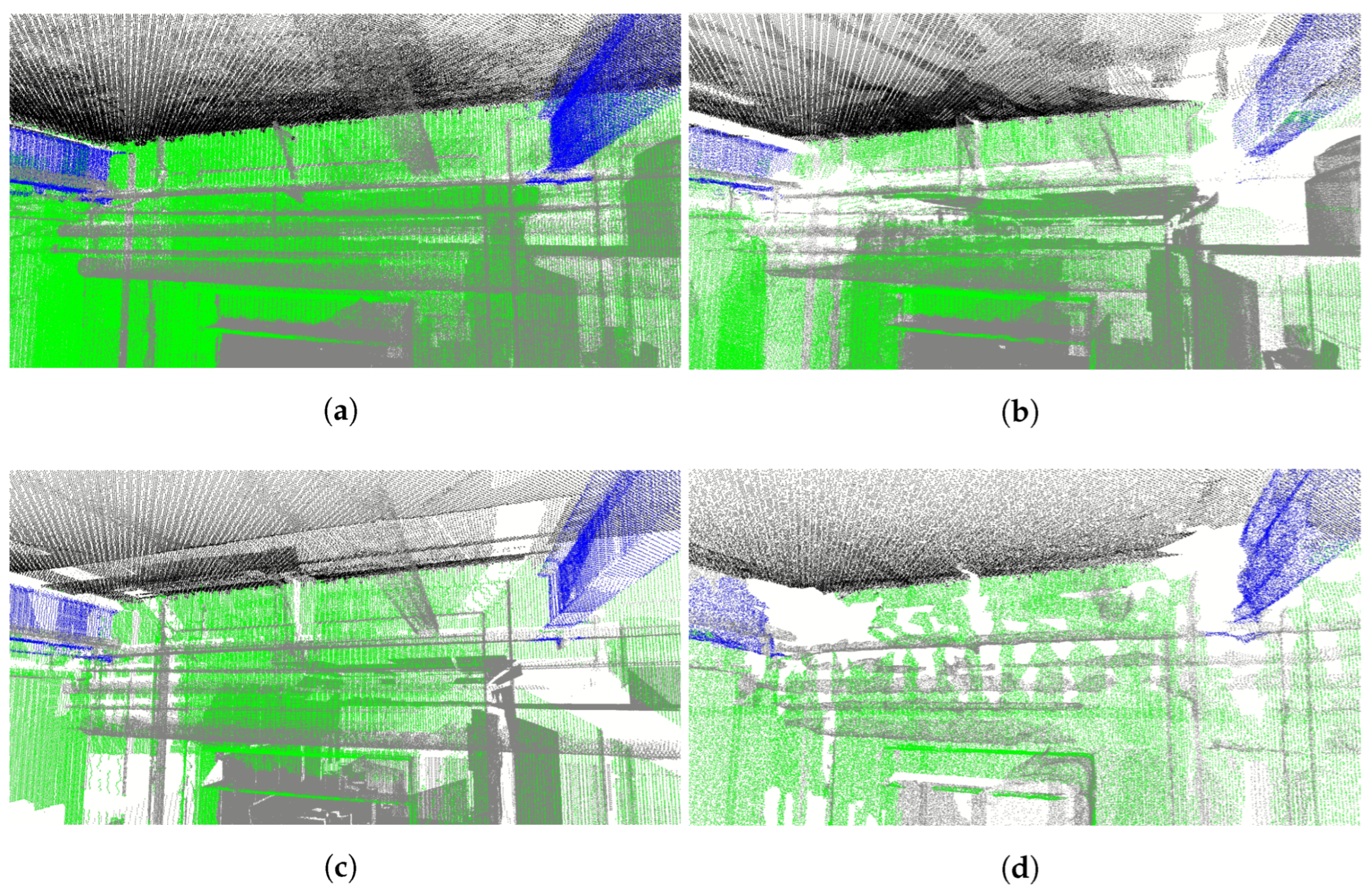
6.2.4. Impact of Semantic Segmentation

For the RandLA-Net processing, every dataset was processed as an unorganized point set with the BIM mesh being sampled up to 0.01 m analogue to the synthetic data. As discussed in the methodology, RandLA-Net was pretrained on Area 6 of the Stanford S3DIS dataset, which consists of a single-storey indoor office/school environment. It is therefore important to notice that lower IoU scores are expected for classes and objects that are not part of this dataset. A very clear indication of this limitation is the poor performance on the synthetic data, which is supposed to resemble a near perfect environment. The generic color, combined with the lack of clutter and unexpected data introduces confusion in the semantic segmentation that was solely trained on real data.
Overall, every dataset was able to be processed by the network at a similar speed as reported by Hu et al. [36]. For the ceilings and floors, all sensors achieve reasonable results (avg. 81%) which is expected given the cross-validation of 93% and 96% of the ceilings and floors of S3DIS Area 6, respectively. However, while in each sensor’s data the main ceiling is easily found, there is significant confusion with lower ceilings and central pieces of the floors. These missclassifications appear in similar locations in all datasets due to training shortcomings of S3DIS. Surprisingly, the lower completeness and quality of the Hololens 2 data do not significantly affect the ceiling or floor classification (Figure 14a).
For the walls, there is a statistical IoU difference between the Hololens 2 and the M6 (avg. 73%), the P30 (65%), and the VLX (58%). However, the results should be nuanced. First of all, the driving factor in the wall IoU is the confusion with clutter observations, especially near wall detailing. The VLX has the highest completeness and thus documents more detailing than other sensors, which in turn leads to higher confusion rates. Second, the wall classification heavily prioritizes precision over recall. As such, relevant parts are found on nearly all wall surfaces without significant false positives for the different sensors which is preferred for general BIM reconstructions (Figure 14b).
For the beams and columns, the results are dramatic, which is expected due to the low cross-validation (beams: 62% and columns: 48%) on Area 6 as a result of limited observations of these classes. For instance, the I-profile in Lab 3 was not found in any sensor data due to a lack of training data (Figure 14c). However, there is an important difference in the classification of each sensor’s data. In Lab 2, the Hololens 2 and P30 only found 2 out of 9 beams, while the M6 and VLX found 5 (Figure 14d). While the Hololens 2 underperforms due to range limitations, the P30 had systematic occlusion gaps which significantly lowered the detection rate. For the columns, it is observed that in the synthetic data, erroneous columns were frequently found near the side faces of the walls where data were also sampled in occluded areas.

7. Discussion

From the experiments, the relation between the point cloud characteristics and the subsequent semantic segmentation can be described. Overall, a high completeness is the most impactful parameter for a successful segmentation, followed by the quality and finally the detailing. For instance, the P30 data has systematic gaps that negatively impact the semantic segmentation of beam parts. However, the impact of all three parameters on the semantic segmentation is rather limited, e.g., in the Hololens 2 data, which in some regions only contains small patches of ceilings, the majority of isolated patches are still properly classified. Similarly, systematic occlusions on floors or walls do not necessarily lead to a worse semantic segmentation. This is also confirmed by other classes and the low discrepancy between IoU statistics in the experiments. If anything, the training data of the model is significantly more impactful, e.g., errors are found near the center of ceilings and floors due to inappropriately trained network weights.
Interestingly, this lack of discrepancy between the classification of different sensor data is extremely beneficiary for developing generalized deep learning models.
For instance, the training data from different sensors can be combined to train a network without having to fear it will not properly train the weights. Further, models that are trained on data from one specific sensor can be used on other sensory data without a significant drop in performance. It is therefore very likely that synthetic training data can be added to the already existing training data and that the model will be further improved. As such, we can make training datasets more balanced and include scenes that would otherwise be very rare in real-world datasets.
Given the above experiments, the points cloud suitability for the BIM structure classes can be compiled for each sensor (Table 7). To this end, expert modelers visually inspected the point clouds and tested whether object class instances their parameters could be reliably set for the different point clouds. It is important to notice that a proper reconstruction requires both suitable point cloud characteristics and that the relevant portions of each object are properly semantically segmented. Overall, the NavVis VLX shows the best results for LOD200-300 reconstructions. This type of portable system is the ideal setup to achieve the highest possible accessibility and have an efficient data acquisition without the need to sacrifice sensor quality due to the weight restrictions. The experiments show that both abstract wall, ceiling, and floor classes as well as details and beam/column types can be reliably extracted up to LOD350 from the classified point clouds conform LOA20 and even LOA30. These systems do need to be supported by total station measurements but the speed of the data acquisition is sufficiently high to merit this approach. In contrast, TLS is still the most qualitative approach and allows modeling up to LOA40. However, this technique struggles to achieve sufficient coverage for LOD350 modeling which also negatively affects the semantic segmentation. Furthermore, TLS generates massive amounts of redundant data in overlapping zones and has disproportionately high detailing compared to its suboptimal coverage. TLS is among the slowest techniques, but its efficiency can be increased when used as a standalone solution which is a suitable approach for mid-scale projects [10]. The NavVis M6 and cart-based systems in general are equally fast as portable systems and offer similar benefits in terms of speed, accuracy, and semantic segmentation. As such, they are outperformed by backpack-based systems that have increased accessibility and thus coverage. Backpack-based systems allow us to map stairs and so connect different datasets, while this is not supported by most cart-based solutions. Overall, these systems in 2021 are a suitable solution for LOD200–350 modeling up to LOA20, and LOA30 if properly supported by TS.
Finally, the Hololens 2 and other head-worn or hand-held devices offer a low-cost alternative to the above high-end systems. Their coverage rivals that of backpack-based systems, although the range is restrictive. Additionally, despite their low data quality, their semantic segmentation is surprisingly good. As such, these systems are capable of LOD200 modeling/analyses up to LOA10 and even LOA20 if properly supported by control measurements or in small areas. Currently, the spatial resolution and the accuracy are the main obstacles to reliably produce LOD300–350 of exact beam/column profiles, accurate wall thickness, etc. Furthermore, the speed is surprisingly low (3× slower than high-end mobile mappers) due to the limited field of view and range that both result in much longer pathing. Overall, these systems are best suited to be used on conjunction with other mapping systems that also provide proper alignment, i.e., standalone TLS or iMMs plus TS.

8. Conclusions

In this paper, the relation between the point cloud data acquisition and the unsupervised data interpretation for as-built BIM modeling/analyses is analyzed to advance the state of the art in point cloud technologies. More specifically, the impact of point cloud data acquisition technologies on the semantic segmentation for structure classes is analyzed. First, the sensor capacity of state-of-the-art data acquisition systems is evaluated for the production of detailed and accurate point cloud data. Secondly, the input point clouds are analyzed for their modeling/analyses suitability conform the LOD and LOA specifications. To this end, the input point clouds are processed by a pretrained RandLA-Net so that, for the first time, the impact of point cloud characteristics on the semantic segmentation are quantified and related to their information extraction suitability.
In the experiments, four types of sensors were tested: static TLS (Leica P30), cart-based iMMs (NavVis M6), backpack-based iMMs (NavVis VLX), and head-worn iMMs (Hololens 2). The point cloud suitability is quantified by the quality, completeness, detailing of the sensor data, and the IoU of the semantic segmentation. Overall, it is concluded that the high-end sensors can be used to model/evaluate geometries up to LOD300-350 by LOA20 and LOA30 if properly supported. Specifically, the NavVis VLX shows the best results for unsupervised point cloud processing automation due to its high coverage and accuracy. Other high-end systems achieve similar results but can struggle with occlusions due lower mobility or slower data acquisition. The low-end Hololens 2 is better suited for close-range LOA10 and LOA20 applications due to its limited range. An important conclusion is that the semantic segmentation is not significantly impacted by the large discrepancies in point cloud characteristics. The accuracy and detailing have little to no impact, and while occlusions do impact the results locally, deep learning networks can overcome this lack of information even for the low-end Hololens 2 data. Overall, we can state that point-based semantic segmentation models do not significantly suffer from differences in the input point clouds. What differences remain can easily be overcome by adding more suitable training data to the network. This poses a great opportunity for 3D data interpretation, as inputs from multiple sensors can be combined to provide much needed deep learning models. As such, the currently scarce and heterogeneous point cloud benchmark datasets can be jointly leveraged. It is important to notice that this sensor invariance also opens the door to synthetic and automatically labeled training data which underexplored for 3D scene interpretation.
This work provides crucial information for researchers and software developers to take into consideration the combined impact of the initial data acquisition and the semantic segmentation and unsupervised point cloud processing for BIM reconstruction/evaluation. Specifically, this work will serve as the basis for future work to build deep learning networks for 3D semantic segmentation that are sufficiently robust for market adoption. The next steps is to generate more (synthetic) data for these networks and investigate whether texture or imagery can offer complementary information to improve the interpretation and reconstruction of heavily occluded building environments.

Author Contributions

S.D.G., J.V., M.B., H.D.W. and M.V. contributed equally to the work. All authors have read and agreed to the published version of the manuscript.

Funding

This project has received funding from the VLAIO BAEKELAND programme (grant agreement HBC.2020.2819) together with MEET HET BV, the VLAIO COOCK project (grant agreement HBC.2019.2509), the FWO Postdoc grant (grant agreement: 1251522N) and the Geomatics research group of the Department of Civil Engineering, TC Construction at the KU Leuven in Belgium.

Institutional Review Board Statement

Not applicable.

Informed Consent Statement

Not applicable.

Data Availability Statement

Not applicable.

Conflicts of Interest

The authors declare no conflict of interest.

References

  1. McKinsey Global Institute. Reinventing Construction: A Route to Higher Productivity; McKinsey Company: Pennsylvania, PA, USA, 2017; p. 20. [Google Scholar] [CrossRef]
  2. Volk, R.; Stengel, J.; Schultmann, F. Building Information Modeling (BIM) for existing buildings—Literature review and future needs. Autom. Constr. 2014, 38, 109–127. [Google Scholar] [CrossRef] [Green Version]
  3. Patraucean, V.; Armeni, I.; Nahangi, M.; Yeung, J.; Brilakis, I.; Haas, C. State of research in automatic as-built modelling. Adv. Eng. Inform. 2015, 29, 162–171. [Google Scholar] [CrossRef] [Green Version]
  4. Wang, W.; Xu, Q.; Ceylan, D.; Mech, R.; Neumann, U. DISN: Deep implicit surface network for high-quality single-view 3d reconstruction. arXiv 2019, arXiv:1905.10711. [Google Scholar]
  5. Mellado, F.; Wong, P.F.; Amano, K.; Johnson, C.; Lou, E.C. Digitisation of existing buildings to support building assessment schemes: Viability of automated sustainability-led design scan-to-BIM process. Archit. Eng. Des. Manag. 2020, 16, 84–99. [Google Scholar] [CrossRef]
  6. Agisoft. Metashape. 2018. Available online: https://www.agisoft.com/ (accessed on 1 January 2022).
  7. Pix4D. Pix4Dmapper. 2021. Available online: https://www.pix4d.com/ (accessed on 1 January 2022).
  8. RealityCapturing. Capturing Reality. 2017. Available online: https://www.capturingreality.com/ (accessed on 1 January 2022).
  9. Remondino, F.; Rizzi, A. Reality-based 3D documentation of natural and cultural heritage sites-techniques, problems, and examples. Appl. Geomat. 2010, 2, 85–100. [Google Scholar] [CrossRef] [Green Version]
  10. Bassier, M.; Yousefzadeh, M.; Genechten, B.V.; Ghent, T.C.; Mapping, M. Evaluation of data acquisition techniques and workflows for Scan to BIM. In Proceedings of the Geo Bussiness, London, UK, 27–28 May 2015. [Google Scholar]
  11. Lagüela, S.; Dorado, I.; Gesto, M.; Arias, P.; González-Aguilera, D.; Lorenzo, H. Behavior analysis of novel wearable indoor mapping system based on 3d-slam. Sensors 2018, 18, 766. [Google Scholar] [CrossRef] [PubMed] [Green Version]
  12. Thomson, C.; Apostolopoulos, G.; Backes, D.; Boehm, J. Mobile Laser Scanning for Indoor Modelling. In Proceedings of the ISPRS Annals of Photogrammetry, Remote Sensing and Spatial Information Sciences, ISPRS Workshop Laser Scanning 2013, Antalya, Turkey, 11–13 November 2013; Volume II-5/W2, pp. 289–293. [Google Scholar] [CrossRef] [Green Version]
  13. Hübner, P.; Clintworth, K.; Liu, Q.; Weinmann, M.; Wursthorn, S. Evaluation of hololens tracking and depth sensing for indoor mapping applications. Sensors 2020, 20, 1021. [Google Scholar] [CrossRef] [Green Version]
  14. Chen, Y.; Tang, J.; Jiang, C.; Zhu, L.; Lehtomäki, M.; Kaartinen, H.; Kaijaluoto, R.; Wang, Y.; Hyyppä, J.; Hyyppä, H.; et al. The accuracy comparison of three simultaneous localization and mapping (SLAM)-based indoor mapping technologies. Sensors 2018, 18, 3228. [Google Scholar] [CrossRef] [Green Version]
  15. Sammartano, G.; Spanò, A. Point clouds by SLAM-based mobile mapping systems: Accuracy and geometric content validation in multisensor survey and stand-alone acquisition. Appl. Geomat. 2018, 10, 317–339. [Google Scholar] [CrossRef]
  16. Tucci, G.; Visintini, D.; Bonora, V.; Parisi, E.I. Examination of indoor mobile mapping systems in a diversified internal/external test field. Appl. Sci. 2018, 8, 401. [Google Scholar] [CrossRef] [Green Version]
  17. Lehtola, V.V.; Kaartinen, H.; Nüchter, A.; Kaijaluoto, R.; Kukko, A.; Litkey, P.; Honkavaara, E.; Rosnell, T.; Vaaja, M.T.; Virtanen, J.P.; et al. Comparison of the selected state-of-the-art 3D indoor scanning and point cloud generation methods. Remote Sens. 2017, 9, 796. [Google Scholar] [CrossRef] [Green Version]
  18. Armeni, I.; Sax, S.; Zamir, A.R.; Savarese, S.; Sax, A.; Zamir, A.R.; Savarese, S. Joint 2D-3D-Semantic Data for Indoor Scene Understanding. arXiv 2017, arXiv:1702.01105. [Google Scholar]
  19. Hackel, T.; Savinov, N.; Ladicky, L.; Wegner, J.D.; Schindler, K.; Pollefeys, M. Semantic3d.Net: A New Large-Scale Point Cloud Classification Benchmark. In Proceedings of the ISPRS Annals of the Photogrammetry, Remote Sensing and Spatial Information Sciences, ISPRS Hannover Workshop: HRIGI 17—CMRT 17—ISA 17—EuroCOW 17, Hannover, Germany, 6–9 June 2017; Volume IV-1-W1. [Google Scholar]
  20. Garcia-Garcia, A.; Orts-Escolano, S.; Oprea, S.; Villena-Martinez, V.; Garcia-Rodriguez, J. A Review on Deep Learning Techniques Applied to Semantic Segmentation. arXiv 2017, arXiv:1704.06857. [Google Scholar]
  21. Xie, Y.; Tian, J.; Zhu, X.X. Linking Points With Labels in 3D: A review of point cloud semantic segmentation. IEEE Geosci. Remote Sens. Mag. 2020, 8, 38–59. [Google Scholar] [CrossRef] [Green Version]
  22. Boulch, A.; Guerry, J.; Le Saux, B.; Audebert, N. SnapNet: 3D point cloud semantic labeling with 2D deep segmentation networks. Comput. Graph. 2018, 71, 189–198. [Google Scholar] [CrossRef]
  23. Wang, K.; Shen, S. MVDepthNet: Real-time multiview depth estimation neural network. In Proceedings of the 2018 International Conference on 3D Vision, 3DV 2018, Verona, Italy, 5–8 September 2018; pp. 248–257. [Google Scholar] [CrossRef] [Green Version]
  24. Dai, A.; Ritchie, D.; Bokeloh, M.; Reed, S.; Sturm, J.; Niebner, M. ScanComplete: Large-Scale Scene Completion and Semantic Segmentation for 3D Scans. In Proceedings of the IEEE Computer Society Conference on Computer Vision and Pattern Recognition, Salt Lake City, UT, USA, 18–23 June 2018; pp. 4578–4587. [Google Scholar] [CrossRef] [Green Version]
  25. Jahrestagung, W.T. Comparison of Deep-Learning Classification Approaches for Indoor Point Clouds. In Proceedings of the 40th Wissenschaftlich-Technische Jahrestagung der DGPF in Stuttgart—Publikationen der DGPF, Stuttgart, Germany, 4–6 March 2020; pp. 437–447. [Google Scholar]
  26. Jiang, M.; Wu, Y.; Zhao, T.; Zhao, Z.; Lu, C. PointSIFT: A SIFT-like Network Module for 3D Point Cloud Semantic Segmentation. arXiv 2018, arXiv:1807.00652. [Google Scholar]
  27. Maturana, D.; Scherer, S. VoxNet: A 3D Convolutional Neural Network for Real-Time Object Recognition. In Proceedings of the IEEE/RSJ International Conference on Intelligent Robots and Systems (IROS), Hamburg, Germany, 28 September–2 October 2015; pp. 922–928. [Google Scholar] [CrossRef]
  28. Tchapmi, L.; Choy, C.; Armeni, I.; Gwak, J.; Savarese, S. SEGCloud: Semantic segmentation of 3D point clouds. In Proceedings of the 2017 International Conference on 3D Vision, 3DV 2017, Qingdao, China, 10–12 October 2017. [Google Scholar] [CrossRef] [Green Version]
  29. Riegler, G.; Ulusoy, A.O.; Geiger, A. OctNet: Learning deep 3D representations at high resolutions. In Proceedings of the 30th IEEE Conference on Computer Vision and Pattern Recognition, CVPR 2017, Honolulu, HI, USA, 21–26 July 2017; pp. 6620–6629. [Google Scholar] [CrossRef] [Green Version]
  30. Wang, P.S.; Liu, Y.; Guo, Y.X.; Sun, C.Y.; Tong, X. O-CNN: Octree-based convolutional neural networks for 3D shape analysis. ACM Trans. Graph. 2017, 36, 72. [Google Scholar] [CrossRef]
  31. Meng, H.Y.; Gao, L.; Lai, Y.K.; Manocha, D. VV-net: Voxel VAE net with group convolutions for point cloud segmentation. In Proceedings of the IEEE International Conference on Computer Vision, Seoul, Korea, 27 October–2 November 2019; pp. 8499–8507. [Google Scholar] [CrossRef] [Green Version]
  32. Qi, C.R.; Su, H.; Mo, K.; Guibas, L.J. PointNet: Deep Learning on Point Sets for 3D Classification and Segmentation. arXiv 2016, arXiv:1612.00593. [Google Scholar]
  33. Qi, C.R.; Yi, L.; Su, H.; Guibas, L.J. PointNet++: Deep Hierarchical Feature Learning on Point Sets in a Metric Space. arXiv 2017, arXiv:1706.02413. [Google Scholar]
  34. Li, Y.; Bu, R.; Sun, M.; Wu, W.; Di, X.; Chen, B. PointCNN: Convolution on X-transformed points. Adv. Neural Inf. Process. Syst. 2018, 31, 820–830. [Google Scholar]
  35. Cai, G.; Jiang, Z.; Wang, Z.; Huang, S.; Chen, K.; Ge, X.; Wu, Y. Spatial aggregation net: Point cloud semantic segmentation based on multi-directional convolution. Sensors 2019, 19, 4329. [Google Scholar] [CrossRef] [PubMed] [Green Version]
  36. Hu, Q.; Yang, B.; Xie, L.; Rosa, S.; Guo, Y.; Wang, Z.; Trigoni, N.; Markham, A. Randla-Net: Efficient semantic segmentation of large-scale point clouds. In Proceedings of the IEEE Computer Society Conference on Computer Vision and Pattern Recognition, Seattle, WA, USA, 13–19 June 2020; pp. 11105–11114. [Google Scholar] [CrossRef]
  37. Hu, Z.; Bai, X.; Shang, J.; Zhang, R.; Dong, J.; Wang, X.; Sun, G.; Fu, H.; Tai, C.L. VMNet: Voxel-Mesh Network for Geodesic-Aware 3D Semantic Segmentation. arXiv 2021, arXiv:2107.13824. [Google Scholar]
  38. Bassier, M.; Vergauwen, M. Unsupervised reconstruction of Building Information Modeling wall objects from point cloud data. Autom. Constr. 2020, 120, 103338. [Google Scholar] [CrossRef]
  39. Yang, F.; Zhou, G.; Su, F.; Zuo, X.; Tang, L.; Liang, Y.; Zhu, H.; Li, L. Automatic indoor reconstruction from point clouds in multi-room environments with curved walls. Sensors 2019, 19, 3798. [Google Scholar] [CrossRef] [PubMed] [Green Version]
  40. Nikoohemat, S.; Diakité, A.A.; Zlatanova, S.; Vosselman, G. Indoor 3D reconstruction from point clouds for optimal routing in complex buildings to support disaster management. Autom. Constr. 2020, 113, 103–109. [Google Scholar] [CrossRef]
  41. Tran, H.; Khoshelham, K.; Kealy, A.; Díaz-Vilariño, L. Shape Grammar Approach to 3D Modeling of Indoor Environments Using Point Clouds. J. Comput. Civ. Eng. 2019, 33, 04018055. [Google Scholar] [CrossRef]
  42. Rebolj, D.; Pučko, Z.; Babič, N.Č.; Bizjak, M.; Mongus, D. Point cloud quality requirements for Scan-vs-BIM based automated construction progress monitoring. Autom. Constr. 2017, 84, 323–334. [Google Scholar] [CrossRef]
  43. U.S. Institute of Building Documentation. USIBD Level of Accuracy (LOA) Specification Guide v3.0-2019; Technical Report; U.S. Institute of Building Documentation: Tustin, CA, USA, 2019. [Google Scholar]
  44. BIMForum. Level of Development Specification; Technical Report; BIMForum: Las Vegas, NV, USA, 2018. [Google Scholar]
  45. U.S. General Services Administration. GSA BIM Guide for 3D Imaging; U.S. General Services Administration: Washington, DC, USA, 2009.
  46. Bonduel, M.; Bassier, M.; Vergauwen, M.; Pauwels, P.; Klein, R. Scan-To-Bim Output Validation: Towards a Standardized Geometric Quality Assessment of Building Information Models Based on Point Clouds. In Proceedings of the ISPRS International Archives of the Photogrammetry, Remote Sensing and Spatial Information Sciences, ISPRS TC II 5th International Workshop LowCost 3D Sensors, Algorithms, Applications, Hamburg, Germany, 28–29 November 2017; Volume XLII-2/W8, pp. 45–52. [Google Scholar] [CrossRef] [Green Version]
  47. Bassier, M.; Vergauwen, M.; Van Genechten, B. Standalone Terrestrial Laser Scanning for Efficiently Capturing Aec Buildings for As-Built Bim. In Proceedings of the ISPRS Annals of Photogrammetry, Remote Sensing and Spatial Information Sciences, Prague, Czech Republic, 12–19 July 2016; Volume III-6, pp. 49–55. [Google Scholar] [CrossRef]
  48. NavVis Gmbh. Confidential: NavVis Mapping Software Documentation; NavVis: Munchen, Germany, 2021. [Google Scholar]
  49. Czerniawski, T.; Leite, F. Automated digital modeling of existing buildings: A review of visual object recognition methods. Autom. Constr. 2020, 113, 103131. [Google Scholar] [CrossRef]
  50. Bassier, M.; Vincke, S.; de Winter, H.; Vergauwen, M. Drift invariant metric quality control of construction sites using BIM and point cloud data. ISPRS Int. J. Geo-Inf. 2020, 9, 545. [Google Scholar] [CrossRef]
  51. NavVis VLX. Evaluating Indoor & Outdoor Mobile Mapping Accuracy; NavVis: Munchen, Germany, 2021; pp. 1–16. [Google Scholar]
Figure 1. Overview of the vital semantic segmentation step that interprets the raw point cloud data and makes it fit for BIM reconstruction.
Remotesensing 14 00582 g001
Figure 2. Overview of the theoretical sensor characteristics.
Remotesensing 14 00582 g002
Figure 3. Overview of the test setup for the sensor capacity tests: (green triangle) starting point (red triangle) end point, (yellow) trajectory and (red) control points of testsite (a) D-hall and (b) E-hall.
Remotesensing 14 00582 g003
Figure 4. Overview of the different test zones that are used for the sensor capacity and point cloud suitability experiments.
Remotesensing 14 00582 g004
Figure 5. Impact of control points on the sensor capacity (D-hall): c2c analysis of the point clouds captured (left) without and (right) with control points compared to the P30 point clouds. Color scale is indicated from 0 m (blue) to 0.1 m (red).
Remotesensing 14 00582 g005
Figure 6. Overview of the Sensor capacity test: Graphs showing the cumulative percentage of c2c-distances between the target and reference point clouds for (a) D-hall: The impact of a control network and (b) E-hall: The impact of loop-closure.
Remotesensing 14 00582 g006
Figure 7. Impact of loop-closure on the sensor capacity (E-hall): c2c analysis of the point clouds captured (left) without and (right) with loop-closure compared to the P30 point clouds. Color scale is indicated from 0 m (blue) to 0.1 m (red).
Remotesensing 14 00582 g007
Figure 8. Alignment shortcomings: Sideview of the Hololens 2 misalignment with sloped floors due the assumptions in the SLAM algorithm (reference point cloud is shown in black). (a) VLX, (b) M6, (c) P30, and (d) Hololens 2.
Remotesensing 14 00582 g008
Figure 9. Coverage shortcomings: The P30 has large systematic occlusions due to limited setups. With the Hololens 2, the ceiling is not recorded due to the limited range of the sensor. The VLX and M6 have higher coverage due to their increased mobility. (a) VLX, (b) M6, (c) P30, and (d) Hololens 2.
Remotesensing 14 00582 g009
Figure 10. Coverage shortcomings: Due to the limited range of the Hololens 2, parts of higher walls cannot be captured properly. (a) VLX, (b) M6, (c) P30, and (d) Hololens 2.
Remotesensing 14 00582 g010
Figure 11. Accessibility shortcomings: Due to the limited space between the obstacles, the P30 and the M6 suffer from large occlusions. (a) VLX, (b) M6, (c) P30, and (d) Hololens 2.
Remotesensing 14 00582 g011
Figure 12. Resolution shortcomings: The Hololens 2 has an order of magnitude lower resolution compared to the other three sensors. This results in narrow or small objects being misinterpreted or missed all together. The VLX and P30 generally have the highest density and give the most dense point cloud which makes it easier to visually identify smaller details. (a) VLX, (b) M6, (c) P30, and (d) Hololens 2.
Remotesensing 14 00582 g012
Figure 13. Detailing shortcomings: Modeling detailed beam profiles from the Hololens 2 data is impossible due to the noise and the reduced resolution. From the data of the high-end devices, the I-profile can be identified. However, the thickness of the body of the profile remains challenging to model due to noise. (a) VLX, (b) M6, (c) P30, and (d) Hololens 2.
Remotesensing 14 00582 g013
Figure 14. Segmentation shortcomings: Problems in the semantic segmentation that are unrelated to the input data. (a) Ceilings are correctly labeled despite large parts of missing data, (b) Due to clutter close to the walls some parts are wrongly labeled, (c) I-profile beam was not recognised in any of the datasets and (d) Rectangular beams are partially found in most datasets.
Remotesensing 14 00582 g014
Table 1. Overview of the Level of Accuracy and Level of Development specification used in Scan-to-BIM methods and their different categories.
Level of AccuracyLOA10LOA20LOA30LOA40LOA50
[0.05 m; −][0.015 m; 0.05 m][0.005 m; 0.015 m][0.001 m; 0.005 m][0; 0.001 m]
Level of Development Remotesensing 14 00582 i001 Remotesensing 14 00582 i002 Remotesensing 14 00582 i003 Remotesensing 14 00582 i004 Remotesensing 14 00582 i005
LOD100LOD200LOD300LOD350LOD400
Table 2. Overview of the BIM modeling/evaluation requirements for structure classes as reported by Wang et al. [4] and Rebolj et al. [42]. The IoU percentual values are directly obtained from Hu et al. [36].
ClassesLevel of
Accuracy
Level of
Development
Quality:
LOA (m)
Completeness:
Coverage (%)
Detailing:
Resolution (m)
Semantic
Segmentation
mIoU S3DIS
(%)
CeilingsLOA20LOD300<0.05>50%<0.0593.1
FloorsLOA20LOD300<0.05>50%<0.0596.1
WallsLOA30LOD350<0.015>50%<0.01580.6
ColumnsLOA30LOD350<0.015>50%<0.01548.0
BeamsLOA30LOD350<0.015>50%<0.01562.4
Table 3. Overview of the number of datasets and time needed with one person to capture and process the data. These times do not include the time needed to establish the TS-network.
NavVis M6NavVis VLXLeica Scanstation P30Microsoft Hololens 2
  D-hallpoints9,998,24717,838,26974,301,732346,206
Capture time±10 min±10 min1 h 45 min±35 min
Process time±20 min±20 min35 min±20 min
  E-hallpoints14,906,83721,411,21949,415,423193,611
Capture time±10 min±10 min1 h 30 min±15 min
Process time±20 min±20 min30 min±20 min
  Lab 1points28,387,57062,441,87170,176,074306,300
Capture time±20 min±20 min±1 h 45 min±27 min
Process time±20 min±20 min±45 min±25 min
  Lab 2points19,855,99532,255,98255,171,563218,790
Capture time±20 min±20 min±1 h 30 min±30 min
Process time±20 min±20 min±30 min±20 min
  Lab 3points17,827,80745,715,87826,501,59993,002
Capture time±10 min±10 min±45 min±20 min
Process time±20 min±20 min±15 min±15 min
Table 4. Results of the point cloud and semantic segmentation testing (Lab 1): Comparative study of the input-validation parameters. Ceilings (black), floors (red), walls (green), beams (blue), and columns (yellow).
Remotesensing 14 00582 i006
QualityCompletenessDetailingSemantic Segmentation
LOA30 (%)LOA20 (%)LOA10 (%)Coverage (%)Resolution (m)IoU (%)
CeilingsSynth----0.0149.6
P3052.987.798.263.50.00369.4
VLX38.186.497.577.60.00470.9
M622.189.197.969.90.00572.2
Hololens 233.489.198.551.30.0572.4
FloorsSynth----0.0139.5
P3093.797.398.323.00.00364.1
VLX56.397.398.839.20.00472.1
M616.492.299.432.30.00576.5
Hololens 227.970.296.829.00.0569.3
WallsSynth----0.0184.9
P3029.779.296.722.90.00355.3
VLX36.580.596.558.30.00453.0
M644.282.295.549.60.00569.5
Hololens 231.779.697.523.40.0569.7
ColumnsSynth----0.010.4
P3053.294.097.944.40.0030.4
VLX47.271.094.865.30.0040.00
M654.896.498.452.30.0050.00
Hololens 217.673.897.847.40.050.00
BeamsSynth----0.017.63
P3065.498.799.659.80.0031.5
VLX58.198.299.283.10.00417.4
M649.198.099.172.20.00536.7
Hololens 231.579.297.755.90.051.3
Table 5. Results of the point cloud and semantic segmentation testing (Lab 2): Comparative study of the input-validation parameters. Ceilings (black), floors (red), walls (green), beams (blue), and columns (yellow).
Remotesensing 14 00582 i007
QualityCompletenessDetailingSemantic Segmentation
LOA30 (%)LOA20 (%)LOA10 (%)Coverage (%)Resolution (m)IoU (%)
CeilingsSynth----0.0149.6
P3051.791.698.943,90.00373.5
VLX36.291.398.974,50.00483.6
M635.791.798.964.80.00587.5
Hololens 210.385.799.241.00.0580.2
FloorsSynth----0.0153.6
P3095.398.299.244.50.00380.3
VLX78.795.298.343.80.00489.2
M647.369.698.336.00.00594.2
Hololens 227.094.998.432.00.0590.8
WallsSynth----0.0185.1
P3038.790.598.839.20.00358.8
VLX48.192.498.669.90.00451.7
M641.588.698.364.20.00567.7
Hololens 227.387.298.235.40.0567.6
ColumnsSynth----0.010.0
P3037.991.096.821.00.0030.1
VLX40.687.297.966.70.0040.0
M643.988.297.953.20.0050.0
Hololens 233.186.098.423.00.050.0
BeamsSynth----0.010.8
P3048.795.799.260.80.0033.3
VLX61.998.899.080.00.00421.2
M660.399.099.270.90.00542.7
Hololens 233.793.699.542.80.053.6
Table 6. Results of the point cloud and semantic segmentation testing (Lab 3): Comparative study of the input-validation parameters. Ceilings (black), floors (red), walls (green), beams (blue), and columns (yellow).
Remotesensing 14 00582 i008
QualityCompletenessDetailingSemantic Segmentation
LOA30 (%)LOA20 (%)LOA10 (%)Coverage (%)Resolution (m)IoU (%)
CeilingsSynth----0.0148.1
P3040.399.899.930.80.00385.3
VLX11.998.398.837.50.00486.7
M626.399.799.834.00.00583.1
Hololens 249.395.297.726.00.0594.6
FloorsSynth----0.0140.4
P3076.199.199.615.00.00391.4
VLX32.593.799.222.00.00489.9
M631.893.299.824.00.00581.2
Hololens 214.496.699.721.00.0594.1
WallsSynth----0.0182.4
P309.846.583.721.00.00379.9
VLX15.060.082.741.00.00470.5
M615.460.083.036.00.00586.2
Hololens 212.948.990.618.00.0581.2
BeamsSynth----0.011.5
P3025.080.997.890.00.0030.0
VLX43.785.497.495.70.0040.0
M646.493.898.781.30.0050.0
Hololens 220.053.091.675.10.050.0
Table 7. Overview of the BIM information that can be extracted from of each scanning technology with regard to the requirements in Table 2.
ClassesLeica P30NavVis VLXNavVis M6Microsoft Hololens 2
CeilingsLOA40/LOD200LOA20-30/LOD300LOA20-30/LOD300LOA10-20/LOD100
FloorsLOA40/LOD200LOA20-30/LOD300LOA20-30/LOD200LOA10-20/LO200
WallsLOA40/LOD300LOA20-30/LOD350LOA20-30/LOD350LOA10-20/LOD200
ColumnsLOA40/LOD300LOA20-30/LOD350LOA20-30/LOD350LOA10-20/LOD100
BeamsLOA40/LOD300LOA20-30/LOD350LOA20-30/LOD350LOA10-20/LOD200
Publisher’s Note: MDPI stays neutral with regard to jurisdictional claims in published maps and institutional affiliations.

