Spatiotemporal Characteristics of the Water Quality and Its Multiscale Relationship with Land Use in the Yangtze River Basin

Abstract

The spatiotemporal characteristics of river water quality are the key indicators for ecosystem health evaluation in basins. Land use patterns, as one of the main driving forces of water quality change, affect stream water quality differently with the variations in the spatiotemporal scales. Thus, quantitative analysis of the relationship between different land cover types and river water quality contributes to a better understanding of the effects of land cover on water quality, the landscape planning of water quality protection, and integrated water resources management. Based on water quality data of 2006–2018 at 18 typical water quality stations in the Yangtze River basin, this study analyzed the spatial and temporal variation characteristics of water quality by using the single-factor water quality identification index through statistical analysis. Furthermore, the Spearman correlation analysis method was adopted to quantify the spatial-scale and temporal-scale effects of various land uses, including agricultural land (AL), forest land (FL), grassland (GL), water area (WA), and construction land (CL), on the stream water quality of dissolved oxygen (DO), chemical oxygen demand (COD_Mn), and ammonia (NH₃-N). The results showed that (1) in terms of temporal variation, the water quality of the river has improved significantly and the tributaries have improved more than the main rivers; (2) in the spatial variation respect, the water quality pollutants in the tributaries are significantly higher than those in the main stream, and the concentration of pollutants increases with the decrease of the distance from the estuary; and (3) the correlation between DO and land use is low, while that between NH₃-N, COD_Mn, and land use is high. CL and AL have a negative effect on water quality, while FL and GL have a purifying effect on water quality. In particular, AL and CL have a significant positive correlation with pollutants in water. Compared with NH₃-N, COD_Mn has a higher correlation with land use at a larger scale. The results highlight the spatial scale and seasonal dependence of land use on water quality, which can provide a scientific basis for land management and seasonal pollution control.

1. Introduction

Freshwater ecosystems, one of the most diverse per unit habitat volumes on earth, play an irreplaceable role in both the natural environment and human society [1]. River networks are connected in both upstream and downstream directions by the stream flow, representing the pathways for mass transport from land to lakes and oceans, which can maintain the connectivity of populations of freshwater species [2]. In a river basin, the quality and quantity of fresh water can determine biodiversity and ecosystem productivity by affecting biogeochemical processes and ecological dynamics [3]. However, with the development of the economy and society in recent years, surface water has been increasingly polluted, which can affect the ecological environment. The quality of life of people, freshwater species, and ecosystems are increasingly threatened by the deteriorating water quality environment [4]. So it is necessary to assess the water quality to protect freshwater ecosystems better. There are many ways to assess the water quality, including water quality index methods [5], water quality models [6], and machine learning [7]. Moreover, with the development of remote sensing technology, many researchers are focusing on remote water quality assessment. For example, Li et al. used remote sensing and the spatial simulated annealing integrated approach to assess the water quality of high dynamic lakes [8]. Şandric et al., based on land cover data, defined a remote measure of the potential of pollution, named RWQ, and showed a good result in water quality assessment [9].

Stream water quality is controlled by both natural and anthropogenic factors, and its relative influence changes with temporal and spatial scales [10,11]. A growing body of research has shown a strong correlation between the type and scale of land use and water quality [12].

Different land use types that reflect the different underlying surface attributes and the intensity of human activities can determine the sources of pollutants flowing into stream flows [13]. A disadvantage of agricultural production is the contamination of the terrestrial environment by atmospheric nitrogen deposition [14]. Agricultural and developed lands are regarded as the main pollution sources of ammonia nitrogen [15]. Agricultural land loses nitrogen easily, and nitrogen fertilizer that cannot be used by crops enters the river with rainfall runoff, causing the nitrogen content to rise [16]. Artificial buildings and impervious surfaces easily gather a large amount of sediment, nutrients, and heavy metal pollutants, which easily flow into rivers and cause a burden on rivers [17]. A decrease in the forest land area or replacement by other land use leads to the deterioration of water quality [18].

The impacts of land use changes on water quality are complex and depend on seasons and spatial scales [19,20,21,22]. In each basin, factors such as the distance of land use from the river, the area of land use, and its spatial distribution on the river affect the water quality of the river [23]. Therefore, the spatial scale where land use has the greatest impact on water quality has always been a research hotspot [24]. Although a large number of studies have proved that land use at different temporal and spatial scales has different impacts on water quality, there is still no unified recognition of which spatial scale has the greatest impact on water quality [25]. For instance, Shi et al. pointed out that the interpretation of the land use pattern on water quality at the riparian scale is higher than that at the watershed scale [26]. Li et al. concluded that as the size of the buffer zone increases, the correlation between construction land and water quality increases, and the positive role of forestland in reducing pollutants increases [27]. In cities, there is a small correlation between farmland and water quality. The reason for these different views is the different natural, socio-economic conditions and different geographical locations in the study areas. In these studies, researchers individually designated the study areas as watershed, sub-catchment, riparian zone, or local area. However, all kinds of factors that affect water quality in different areas of an entire river basin lead to different spatial scales and different buffer zones that have various effects on water quality. It indicates that instead of dividing different areas into buffer zones or watersheds, combining them is more reasonable and desirable when identifying the correlation between water quality and land use in the entire basin.

The Yangtze River basin is one of the most densely populated areas in China. Surface runoff plays an important role in the ecological environment and human water use. However, the water security in the basin is under increasing threat. Understanding the relationship between land use and water quality in the Yangtze River basin can provide a scientific basis for water pollution control and land use management. In the Yangtze River basin, many researchers have studied the relationship between land use and water quality, and their research areas were mainly concentrated in the Three Gorges [28], the Han River [29], and the Yangtze River delta [30]. They thought there is a strong correlation between land use and water quality, but most of them did not consider the influence of different temporal and spatial scales on the correlation. Some scholars have considered the effect of the spatial scale on the correlation changes from watershed to riparian [25,31], ignoring the correlation changes from riparian to watershed. In this study, the relationship between land use and water quality is studied in different subregions in the whole Yangtze River basin by dividing the buffer from the more sophisticated space scale and more comprehensive timescales, and thus a more comprehensive discussion is conducted of the factors affecting water quality. The main aims of this study are (1) to detect the spatiotemporal variations in the water quality of the basin, (2) to analyze land use changes, (3) and to evaluate the impact of different land uses on river water quality at the watershed and buffer scale in the whole Yangtze River basin.

2. Materials and Methods

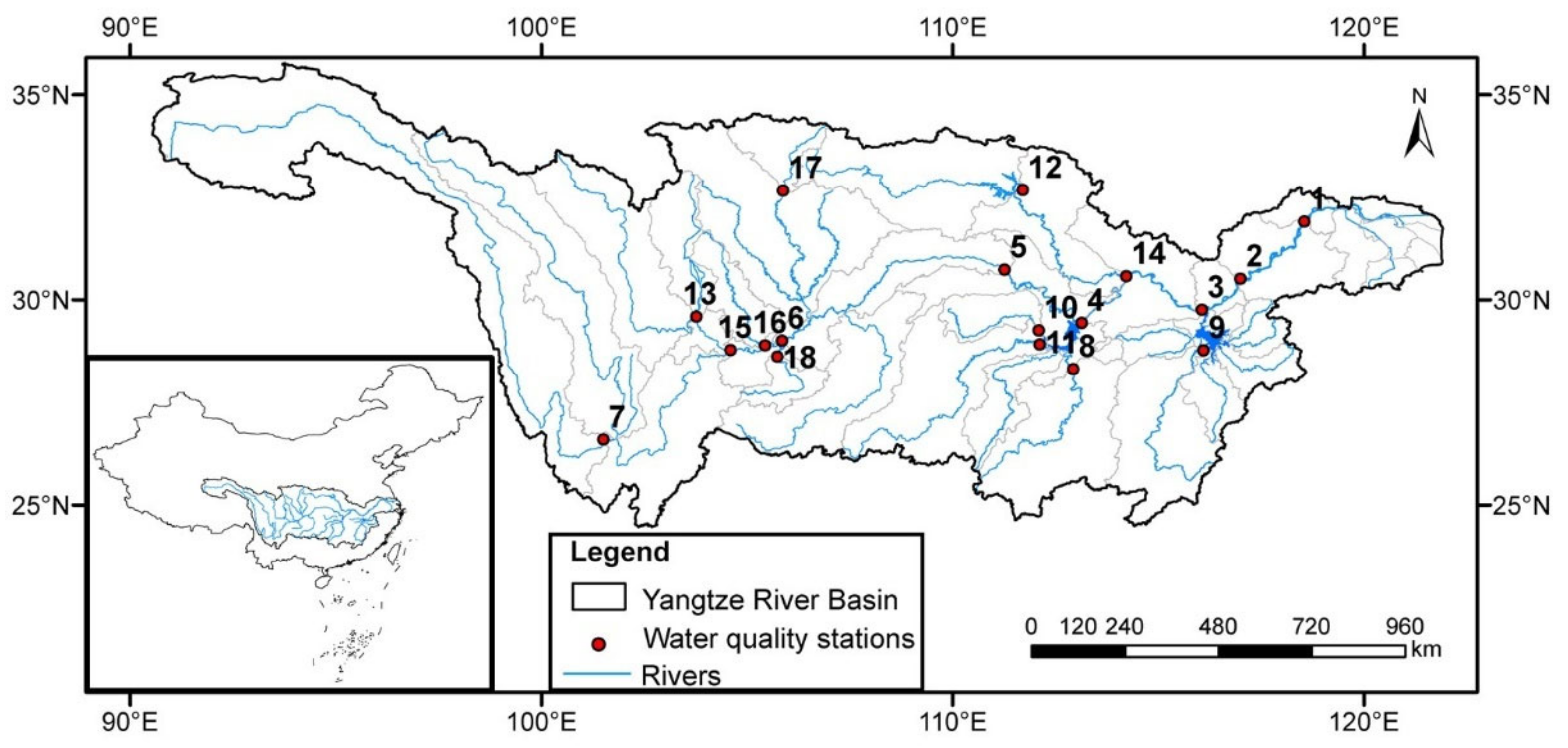
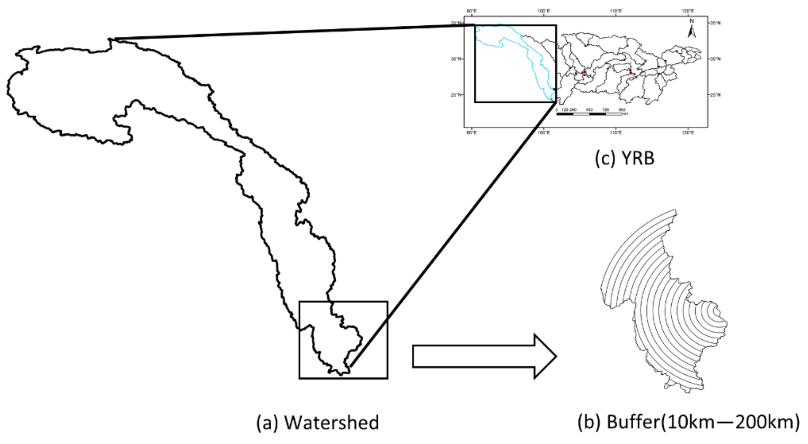
2.1. Study Area

Located at 24° to 35° north latitude and 90° to 122° east longitude, the Yangtze River basin (YRB) (Figure 1) is the third-largest basin in the world, including vast main streams and tributaries, spanning 19 provinces, cities, and autonomous regions in east, central, and west China. The total area of the basin is 1.8 million km², accounting for 18.8% of China’s land area [32]. The YRB is a multilevel ladder terrain. It flows through mountains, plateaus, basins (tributaries), hills, and plains, as well as the Qinghai Tibet Plateau, Hengduan Mountains, Yunnan Guizhou Plateau, Sichuan Basin, Jiangnan Hills, and the plains of the middle and lower reaches of the Yangtze River. The YRB can be divided into three geographical climate regions: the Qinghai Tibet high cold region in the west, the tropical monsoon climate region in the southwest, and the subtropical monsoon climate region [33]. The main stream length of the Yangtze River is 6397 km, with a total basin area of about 1.8 million km², accounting for 18.8% of China’s land area. The upper reach of the main stream of the Yangtze River is above Yichang, with a drainage area of 1 million km². The middle reach of the Yangtze River is from Yichang to Hukou, with a drainage area of 0.68 million km². The lower reach is below Hukou, with a drainage area of 0.12 million km². The number of cities and urban built-up area in the YRB generally increased, and the expansion was the most dramatic from 2006 to 2013 [34]. Water quality in the basin has improved in recent years, while the pollution levels are still relatively high due to industrial and domestic wastewater discharge in the regions with higher GDP and population density [35].

2.2. Data

2.2.1. Water Quality Dataset and Indicators Selection

In this study, the weekly measured water quality concentrations at 18 water quality stations (

Table 1. Basic information of water quality sites in Yangtze River Basin.

ID	Station Name	River	NS	Period
1	Linshan	Yangtze River	144	2006–2018
2	Wanhekou	Yangtze River	144	2006–2018
3	Hexi Drinking Water Plant	Yangtze River	144	2006–2018
4	Chenglingji	Yangtze River	144	2006–2018
5	Nanjinguan	Yangtze River	144	2006–2018
6	Zhutuo	Yangtze River	144	2006–2018
7	Longdong	Yangtze River	144	2006–2018
8	Xingang	Xiangjiang River	144	2006–2018
9	Chucha	Ganjiang River	144	2006–2018
10	Shahekou	Lishui River	84	2011–2018
11	Potou	Yuanjiang River	72	2012–2018
12	Taocha	Hanjiang River	144	2006–2018
13	Minjiang Bridge	Minjiang River	144	2006–2018
14	Zongguan	Hanjiang River	144	2006–2018
15	Liangjianggou	Minjiang River	144	2006–2018
16	Tuojiang Second Bridge	Tuojiang River	144	2006–2018
17	Qingfengxia	Jialing River	132	2007–2018
18	Lianyuxi	Chishui River	84	2011–2018

NS denotes the number of samples obtained at each station, and “Period” denotes the period in which the data are covered (2017 data are missing).

) during 2006 to 2016 and 2018 were collected according to the geographical location and area of the main tributaries of the Yangtze River basin from the China National Environmental Monitoring Center (http://www.cnemc.cn; accessed on 12 November 2020). Three water quality indicators, dissolved oxygen (DO), chemical oxygen demand (COD_Mn), and ammonia (NH₃-N), were selected for analysis, which have been most commonly and widely used to represent stream water quality [13]. The original data we obtained were weekly data. Through statistical processing, we averaged the weekly data in each month to get the monthly data and the average of the weeks of the year to get the annual average. Seventy percent of the precipitation in the Yangtze River Basin occurs from April to October [36]. So we defined the wet season as April to October and the dry season as November to March. The data of the wet season are the average of monthly data from April to October. The data of the dry season are the average of monthly data from November to March. For analysis with land use data, water quality data were divided into four stages. The water quality data for each stage were averaged from annual and seasonal data included in the stage. The range of years for the stages of each water quality station is shown in

Table 2. The range of years for each stage.

ID	Station Name	Stage 1	Stage 2	Stage 3	Stage 4
1	Linshan	2006–2008	2010–2012	2013–2015	2016,2018
2	Wanhekou	2006–2008	2010–2012	2013–2015	2016,2018
3	Hexi Drinking Water Plant	2006–2008	2010–2012	2013–2015	2016,2018
4	Chenglingji	2006–2008	2010–2012	2013–2015	2016,2018
5	Nanjinguan	2006–2008	2010–2012	2013–2015	2016,2018
6	Zhutuo	2006–2008	2010–2012	2013–2015	2016,2018
7	Longdong	2006–2008	2010–2012	2013–2015	2016,2018
8	Xingang	2006–2008	2010–2012	2013–2015	2016,2018
9	Chucha	2006–2008	2010–2012	2013–2015	2016,2018
10	Shahekou	–	2011–2012	2013–2015	2016,2018
11	Potou	–	2012	2013–2015	2016,2018
12	Taocha	2006–2008	2010–2012	2013–2015	2016,2018
13	Minjiang Bridge	2006–2008	2010–2012	2013–2015	2016,2018
14	Zongguan	2006–2008	2010–2012	2013–2015	2016,2018
15	Liangjianggou	2006–2008	2010–2012	2013–2015	2016,2018
16	Tuojiang Second Bridge	2006–2008	2010–2012	2013–2015	2016,2018
17	Qingfengxia	2007–2008	2010–2012	2013–2015	2016,2018
18	Lianyuxi	–	2010–2012	2013–2015	2016,2018

.

2.2.2. Land Use Dataset

In this paper, the land use grid maps at 1 km × 1 km resolution of the years 2005, 2010, 2015 and 2018 were selected from Landsat TM/ETM remote sensing image calibration at the Resource and Environmental Science Data Center of Chinese Academy of Sciences (http://www.resdc.cn/; accessed on 12 November 2020). To better investigate the relationships between water quality and land use, the land use types in the study area were reclassified and divided into six types according to the National Land Classification Standard: agricultural land (AL), forest land (FL), grassland (GL), water area (WA), construction land (CL), and unused land (UL).

Since the composition and change of all land use in the upstream area of the water quality station have a direct or indirect impact on the water quality, we defined the range of sub-basins affecting the water quality at each station as the sum of all sub-basins in the upstream region of the station that conform to the production and confluence mechanism. Considering that the Yangtze River basin has a large area and the land use grid map used is at 1:100,000 scale, we created 10–200 km multi-ring circular buffers at the center of each site and then cropped them along the watershed boundary. In addition, land use changes were analyzed in different buffer zones in the sub-basins where the water quality stations are located. Taking Longdong Station as an example, the division of the basin and each buffer zone is shown in Figure 2.

2.3. Methods

2.3.1. Single-Factor Water Quality Identification Index

The single-factor water quality identification index can completely mark important information, such as the category of the water quality evaluation index, water quality data, and functional area target value, which can not only qualitatively evaluate according to the national standard category but also analyze water quality data according to the labeling index. The difference in the same type of water quality index in the same grade can be compared and analyzed, and the pollution degree of water quality can be compared and analyzed in different types of water quality indexes [37].

The single-factor water quality index P consists of one integer, with two or three significant digits after the decimal point, and is expressed as

$$P_i=X_1.X_2{X}_3,$$

(1)

where X₁ represents the water quality category of the water quality index in item i (the larger the value, the more serious the water pollution of the monitoring index); X₂ represents the position of monitoring data in the change interval of grade X₁ water quality, which is determined by the principle of rounding according to the formula; and X₃ represents the comparison result between the water quality category and the set category of the water function area and is the pollution degree of the evaluation index. X₃ is one or two valid numbers (according to the research needs of this paper, the single-factor water quality index adopted one integer and one significant digit after the decimal point).

According to the evaluation standard of environmental quality standards for surface water (GB 3838-2002), when the water quality is between grades I and V, the non-dissolved oxygen index is as follows:

$$X_1.X_2=k+\frac{{\rho }_{\mathrm{i}}-{\rho }_{i,k\downarrow }}{{\rho }_{i,k\uparrow }-{\rho }_{i,k\downarrow }}$$

(2)

The index of dissolved oxygen is as follows:

$$X_1.X_2=k+1-\frac{{\rho }_{\mathrm{i}}-{\rho }_{i,k\downarrow }}{{\rho }_{i,k\uparrow }-{\rho }_{i,k\downarrow }},$$

(3)

where k = 1, 2, 3, 4, and 5 and represents the indexes of grade I, grade II, grade III, grade IV, and grade V, respectively. ${\rho }_i$ is the index of item i measured concentration; ${\rho }_{i,k\uparrow }$ and ${\rho }_{i,k\downarrow }$ are the upper and lower limits of the water quality standard interval in the water quality index of item i in grade k, respectively.

When the water quality is worse than or equal to the grade V water limit, the non-dissolved oxygen index is as follows:

$$X_1.X_2=6+\frac{{\rho }_{\mathrm{i}}-{\rho }_{i,5\uparrow }}{{\rho }_{i,5\uparrow }}$$

(4)

The index of dissolved oxygen is as follows:

$$X_1.X_2=6+\frac{{\rho }_{DO,5\downarrow }-{\rho }_{DO}}{{\rho }_{DO,5\downarrow }}\times 4$$

(5)

where ${\rho }_{i,5\uparrow }$ and ${\rho }_{i,5\downarrow }$ are the upper and lower limits of the standard interval of the water quality index of item i in grade V, respectively.

2.3.2. The Mann–Kendall Trend Test

The Mann–Kendall trend test is based on the correlation between the ranks of a time series and their time order [38,39,40]. For a time series A = {a₁, a₂,…, a_n}, the calculation process of this method is as follows:

Comparing the water quality data of each year in year i, if the second year is greater than the first year, marked as +1, and vice versa as −1, no change is recorded as 0, and the sum of the counts for all years is obtained as follows:

$$S={\displaystyle \sum _{i<j}sign(a_j-a_i)}$$

(6)

$$sign(a_j-a_i)=\left\{\begin{array}{ll}1& a_j>a_i\\ 0& a_j=a_i\\ -1& a_j<a_i\end{array}\right.$$

(7)

Under the null hypothesis, Var(S_n) is

$$Var\left(S_n\right)=\frac{n\left(n-1\right)\left(2n+5\right)}{72},$$

(8)

where n is the number of observations. The existence of tied ranks (equal observations) in the data results in a reduction in the variance of Var to become

$$Var\left(S_n\right)=\frac{n\left(n-1\right)\left(2n+5\right)}{72}-{\displaystyle \sum _{i=1}^m{t}_j(t_j-1)}(2t_j+5)/18,$$

(9)

where m is the number of groups of tied ranks.

The formula for calculating the statistical test value Z is

$$Z=\left\{\begin{array}{ll}(S-1)/\sqrt{Var(s)}& if S>0\\ 0& if S=0\\ (S-1)/\sqrt{Var(s)}& if S<0\end{array}\right..$$

(10)

When Z > 0, the sequence has an upward trend; when Z < 0, the sequence has a downward trend; if |Z| < 1.96, the change is not significant; if 1.96 < |Z| < 2.56, the change is significant; if |Z| > 2.56, the change is extremely significant; and the greater the value of |Z|, the more significant the change.

2.3.3. Spearman Rank Correlation

The Spearman rank correlation coefficient is a statistical method used to evaluate the correlation between two variables. The most prominent feature is that there is no need to examine the sample size or overall distribution characteristics of variables, which is fast and robust. For two vectors X and Y with dimension n, X_i and Y_i represent their corresponding i (1 ≤ I ≤ n) elements, respectively. X and Y are arranged in the same ascending or descending order to get a new sequence of variables x and y. Among them, x_i is the rank of x_i in x and y_i is the rank of y. Correspondingly, the difference set d_i = x_i − y_i defines the Spearman rank correlation coefficient between the random variables X and Y as follows [41]:

$$\mathrm{r}=1-\frac{6{\displaystyle {\sum }_{i=1}^n{d}_i^2}}{n(n^2-1)}$$

(11)

The numerator is the sum of the errors between two sequences, reflecting the differences between the two variables; the denominator is a constant related to the length of the sequence. From the calculation process, it can be seen that the calculation of the Spearman rank correlation coefficient has few restrictions and high efficiency. It has been applied for many times in the study of correlation between land use and water quality.

We extracted the land use data of the watershed boundary of the sub-watershed where each station is located, and used the Spearman correlation analysis method to establish and analyze the correlation between the area proportion of land use types and water quality indicators so as to qualitatively determine the impact of land use types on water quality.

3. Results

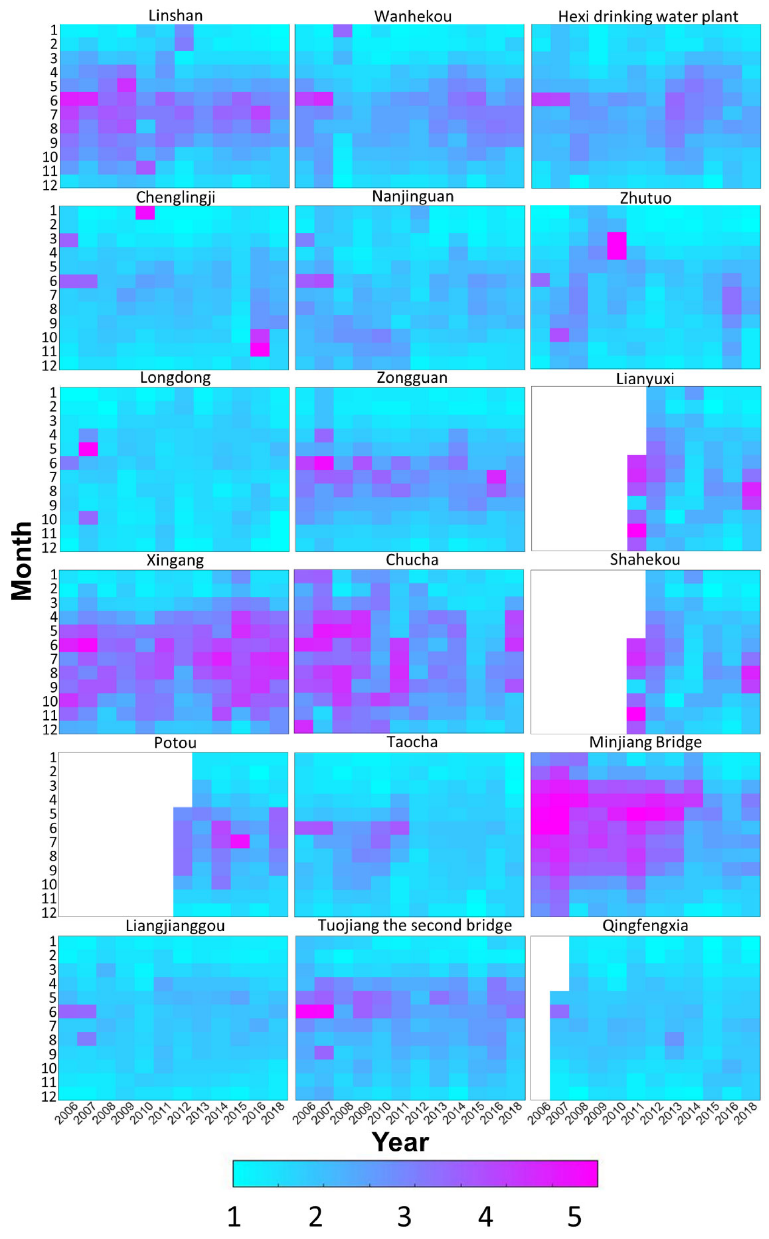
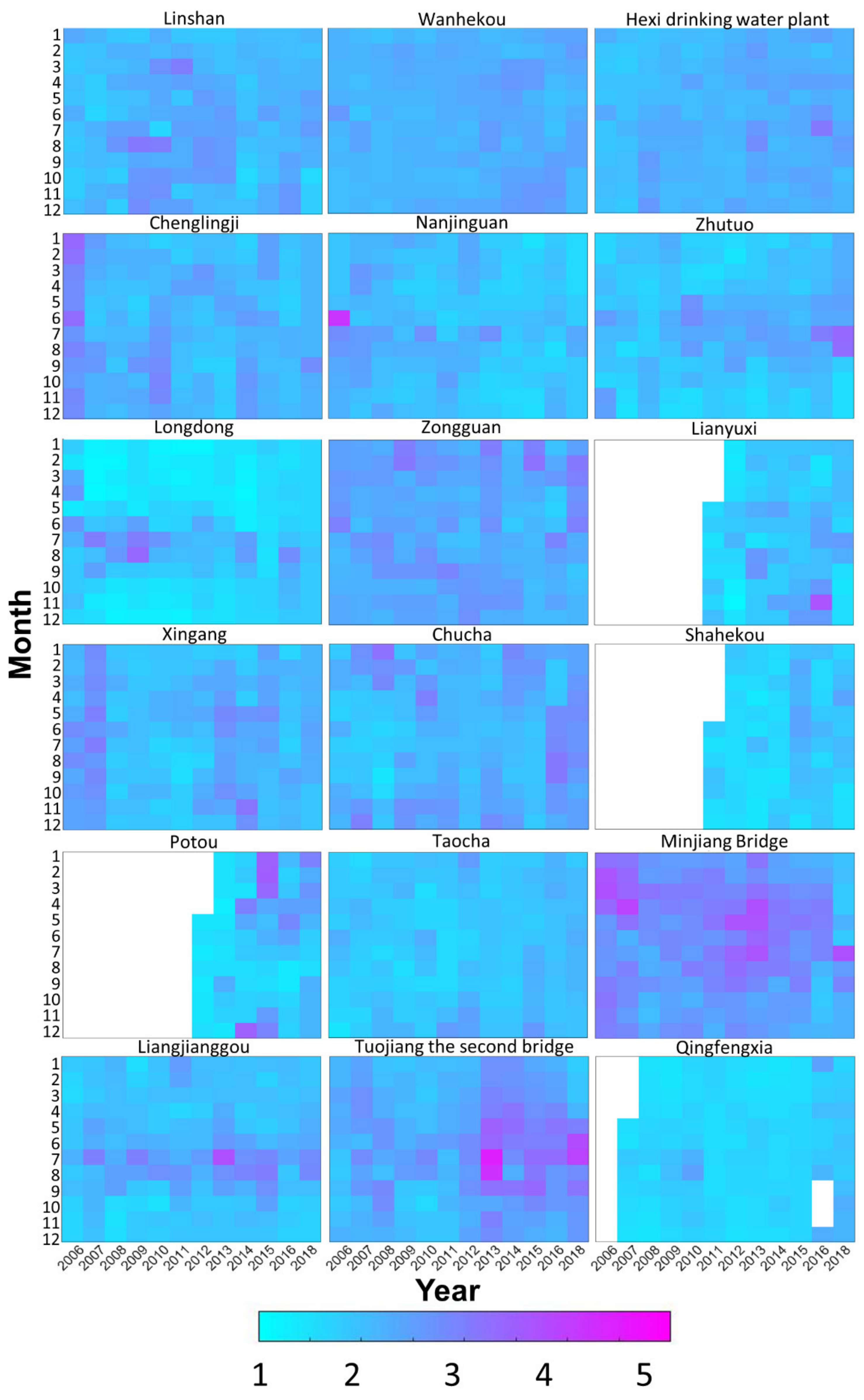
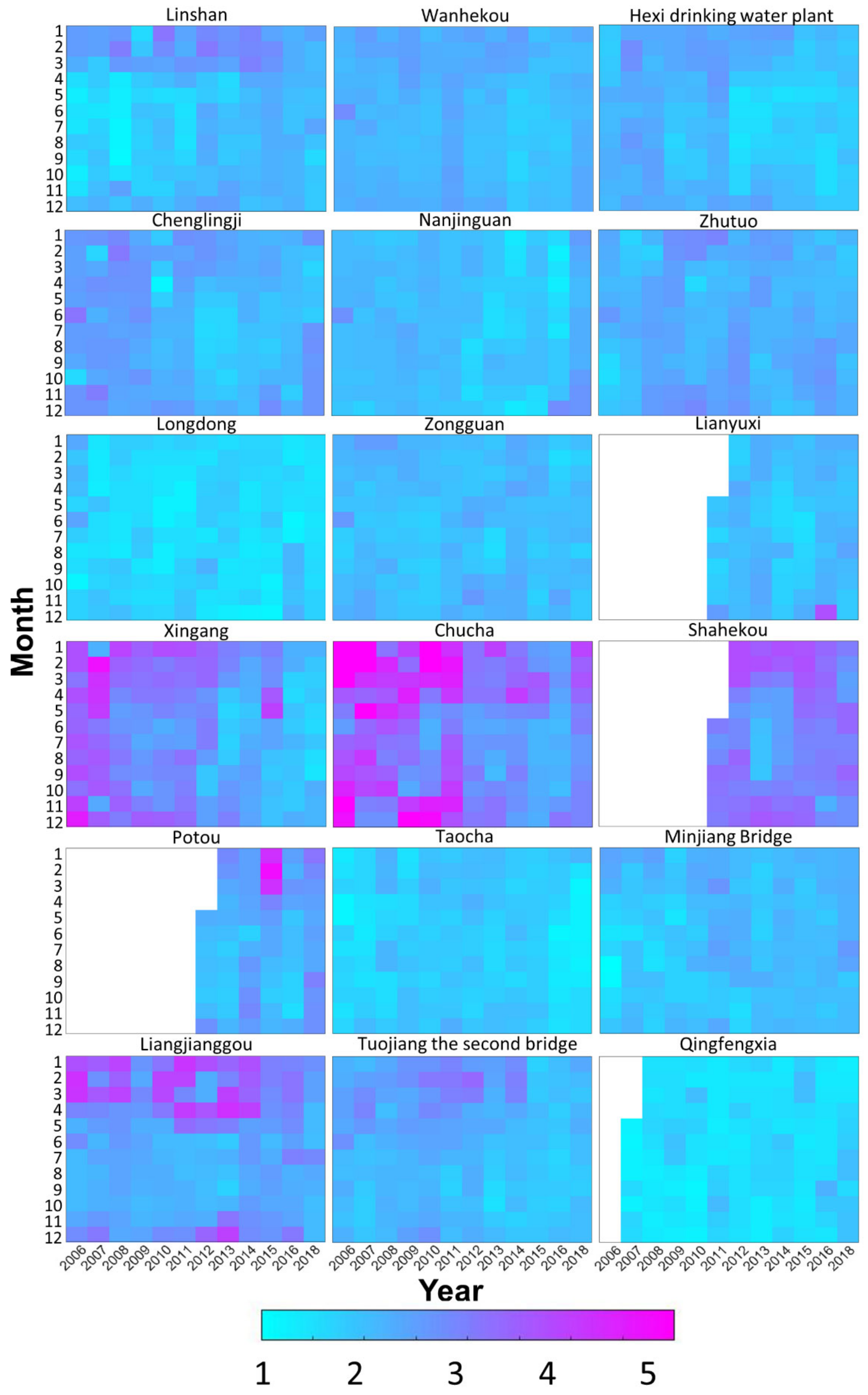
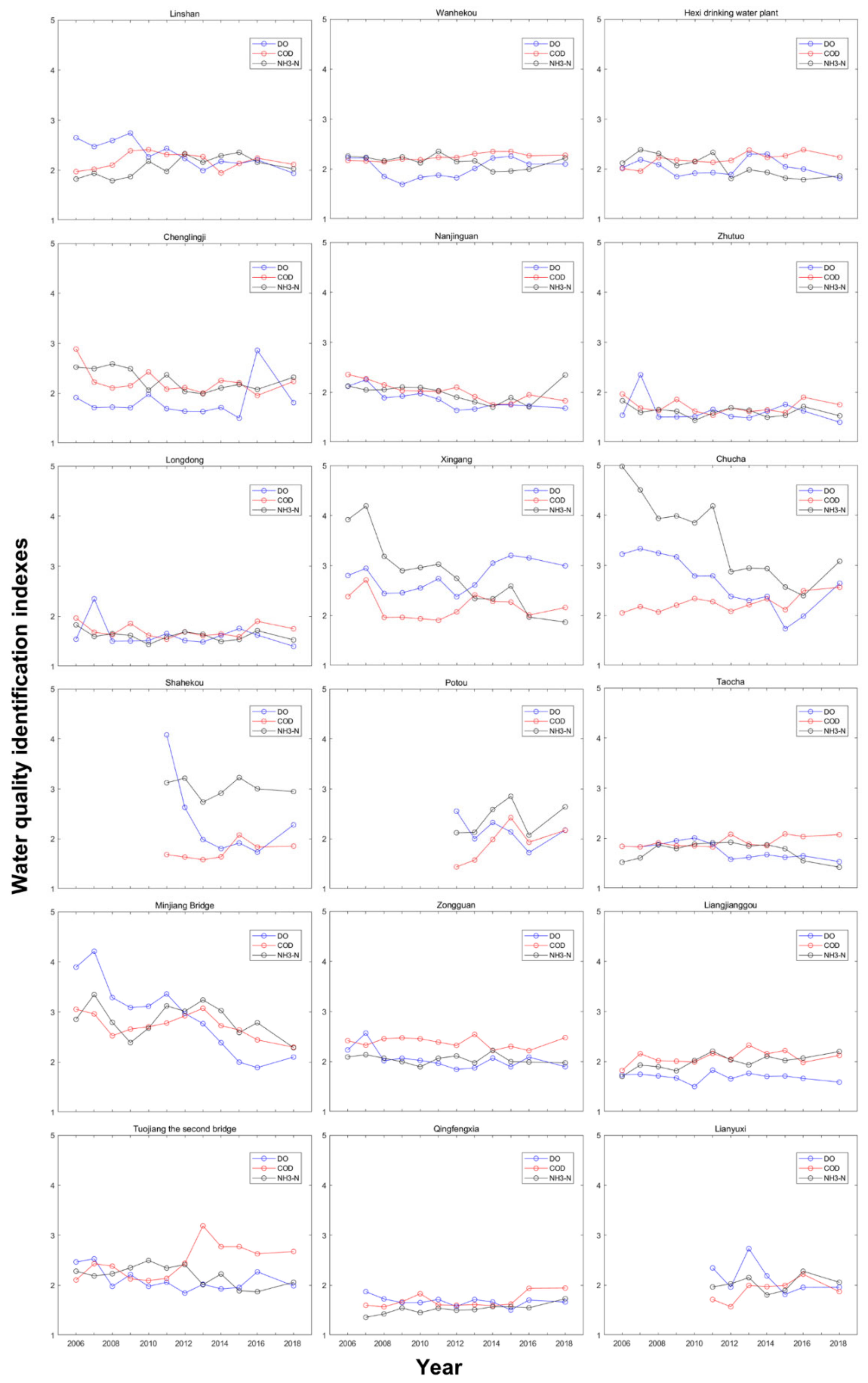
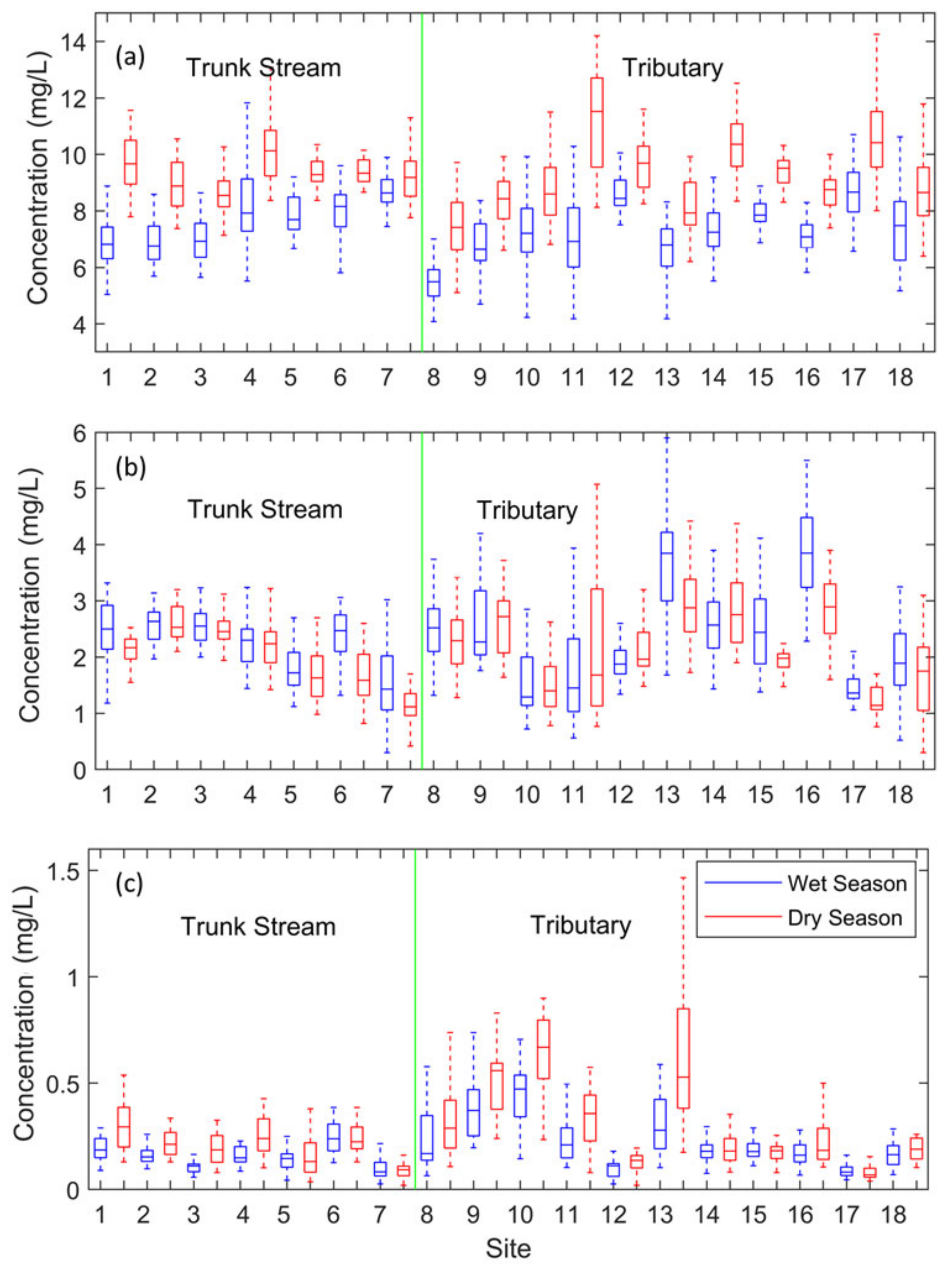
3.1. Spatiotemporal Characteristics of the Water Quality

To reveal the seasonal variation characteristics of water quality, the monthly mean water quality data from 2012 to 2018 of 18 stations in the wet season (April–October) and the dry season (November–March of the next year) were compared and analyzed. As shown in Figure 3, Figure 4, Figure 5 and Figure 6, water quality was characterized by seasonal changes. The seasonal variation of DO was high, and it can be seen that the concentration of DO in the dry season was significantly higher than that in the wet season at each site, especially in Linshan, Chucha, Xingang, and Minjiang Bridge. It can be clearly seen that water quality reached grade II or even grade I in the dry season, while water quality deteriorated to grade III or grade IV in the wet season. In the wet season, there were obvious spatial variations in the main stream, and the concentration of DO increased with the increase in distance from the estuary. The concentration of NH₃-N varied greatly by season, with a high concentration in the dry season and al ow concentration in the wet season. In the wet season, precipitation and the river flow were high, which resulted in the dilution of DO in the water. In contrast to DO, NH₃-N showed poor water quality in the dry season and good water quality in the wet season. This was obvious in Chucha, Minjiang Bridge, and Xingang. Compared with most of the tributaries, the concentration of NH₃-N in the trunk stream was significantly lower, but the concentration of NH₃-N in the trunk stream was higher in the Xiangjiang River, Yuanjiang River, Lishhui River, and Minjiang River. The seasonal variation in the COD_Mn concentration at each station was slight, and the concentration at most stations was higher in the wet season than in the dry season. Compared with DO and NH₃-N, although the seasonal variation in COD was not so obvious, it can be seen from Longdong, Minjiang Bridge, Tuojiang Second Bridge, and Liangjianggou stations that the water quality in the wet season was worse than that in the dry season. The spatial distribution of the COD_Mn concentration in the trunk stream was obviously different. As the distance from the estuary decreased, the concentration of COD_Mn increased, which may be caused by the fact that COD_Mn is not easily adsorbed by soil and the pollutants accumulate along the river basin. The concentration of COD_Mn was different in different tributaries. The values were higher in the Minjiang River and Tuojiang River than in the other basins.

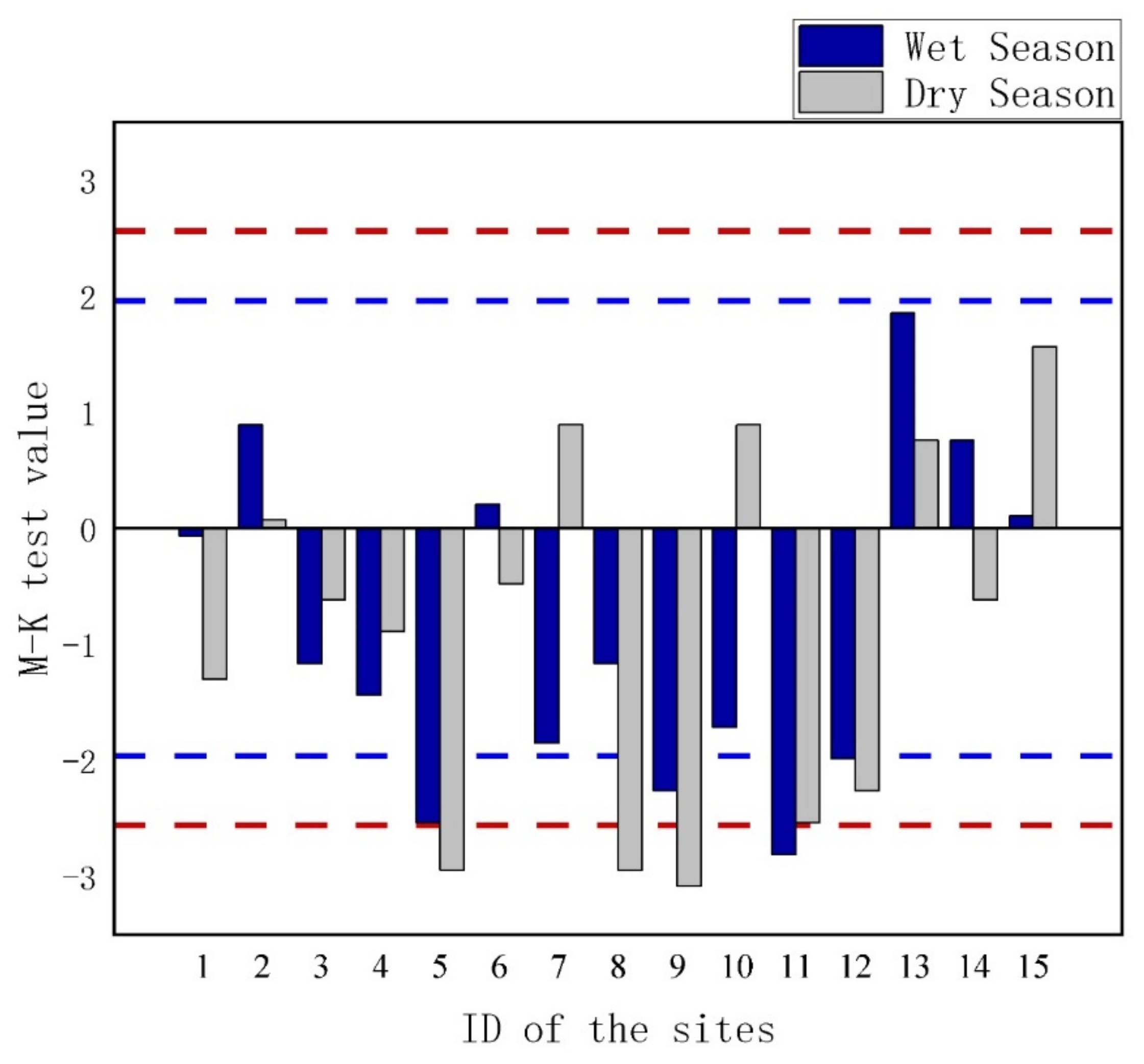
3.2. Analysis of Annual Trend of Water Quality

As shown in Figure 6, the change in water quality in the main stream was relatively stable, fluctuating around grade II. DO fluctuated up and down in five sites: Zhutuo, Wanhekou, Longdong, Chenglingji, and Hexi Drinking Water Plant. The DO in two sites, Nanjinguan and Linshan, had a significant downward trend. COD_Mn fluctuated up and down in five sites, Zhutuo, Wanhekou, Longdong, Linshan, and Hexi Drinking Water Plant, and decreased significantly in two sites, Nanjinguan and Chenglingji. NH₃-N fluctuated up and down in four sites, Zhutuo, Wanhekou, Longdong, and Linshan, while eight sites, including Nanjinguan, Hexi Drinking Water Plant, and Chenglingji, showed an obvious trend of decline.

The water quality of tributaries changed more than that of the main streams. By 2018, the water quality could basically meet the standards of grade II or grade III. DO showed an obvious declining trend in eight sites: Chucha, Shahekou, Potou, Lianyuxi, Zongguan, Taocha, Tuojiang Second Bridge, and Minjiang Bridge. DO in the other three sites fluctuated up and down. The COD_Mn in two sites, Xingang and Minjiang Bridge, showed an obvious declining trend. The COD_Mn in eight sites (Chucha, Shahekou, Lianyuxi, Zongguan, Taocha, Tuojiang Second Bridge, Qingfengxia, and Liangjianggou) showed a fluctuating trend or a slightly upward trend, while in Potou, it showed a significant upward trend. NH₃-N showed an obvious downward trend in four sites (Chucha, Tuojiang Second Bridge, Minjiang Bridge, and Xingang), and in seven sites (Shahekou, Potou, Lianyuxi, Zongguan, Taocha, Qingfengxia, and Liangjianggou), NH₃-N fluctuated up and down.

To reveal the changes in water quality in different seasons, we weighted and averaged all kinds of water quality evaluation factors to obtain a comprehensive water quality index and conducted an MK trend test for the dry season and the wet season. Due to the short time series of water quality data of Shahekou, Potou, and Lianyuxi, we conducted the MK trend test to eliminate them. As shown in Figure 7, it can be seen that the water quality index of tributaries had a significantly higher downward trend than that of the main streams. In the dry season, the water quality indexes of six sites showed an upward trend but did not reach the significance level of 0.05, which is not an obvious upward trend, while the water quality indexes of nine sites showed a downward trend, and five sites exceeded the significance level of 0.05, showing a significant downward trend. In the wet season, the water quality indexes of five sites showed an upward trend, but did not reach the significance level of 0.05. The water quality indexes of 10 sites showed a downward trend, and 4 sites showed a significant downward trend. From the point of view of stations showing a significant downward trend, except for Minjiang Bridge, the downward trend in the dry season was obviously greater than that in the wet season.

On the whole, the water quality of the whole Yangtze River basin is dominated by grade II and grade III. The water quality of some sites can reach grade I, and before 2010, the water quality of a few sites reached grade IV, but by 2018, the water quality of all sites improved significantly and was basically maintained at the level of grade II or grade III. All kinds of water quality mainly showed up and down fluctuations or obvious downward trends, but different water quality categories in different regions reflected different trends. The water quality of the main stream was obviously better than that of the tributaries, and the water quality indexes fluctuated up and down at most sites. Some of the water quality indexes in tributaries showed a downward trend, especially NH₃-N and DO indexes. Although the water quality of some sites had a certain upward trend, it could still reach grade II. Although the water quality of the tributary is not as good as that of the main stream, it can be seen from trend analysis that the changing trend in the water quality of the tributary is more obvious. The trend in water quality improvement in the dry season is obviously higher than that in the wet season.

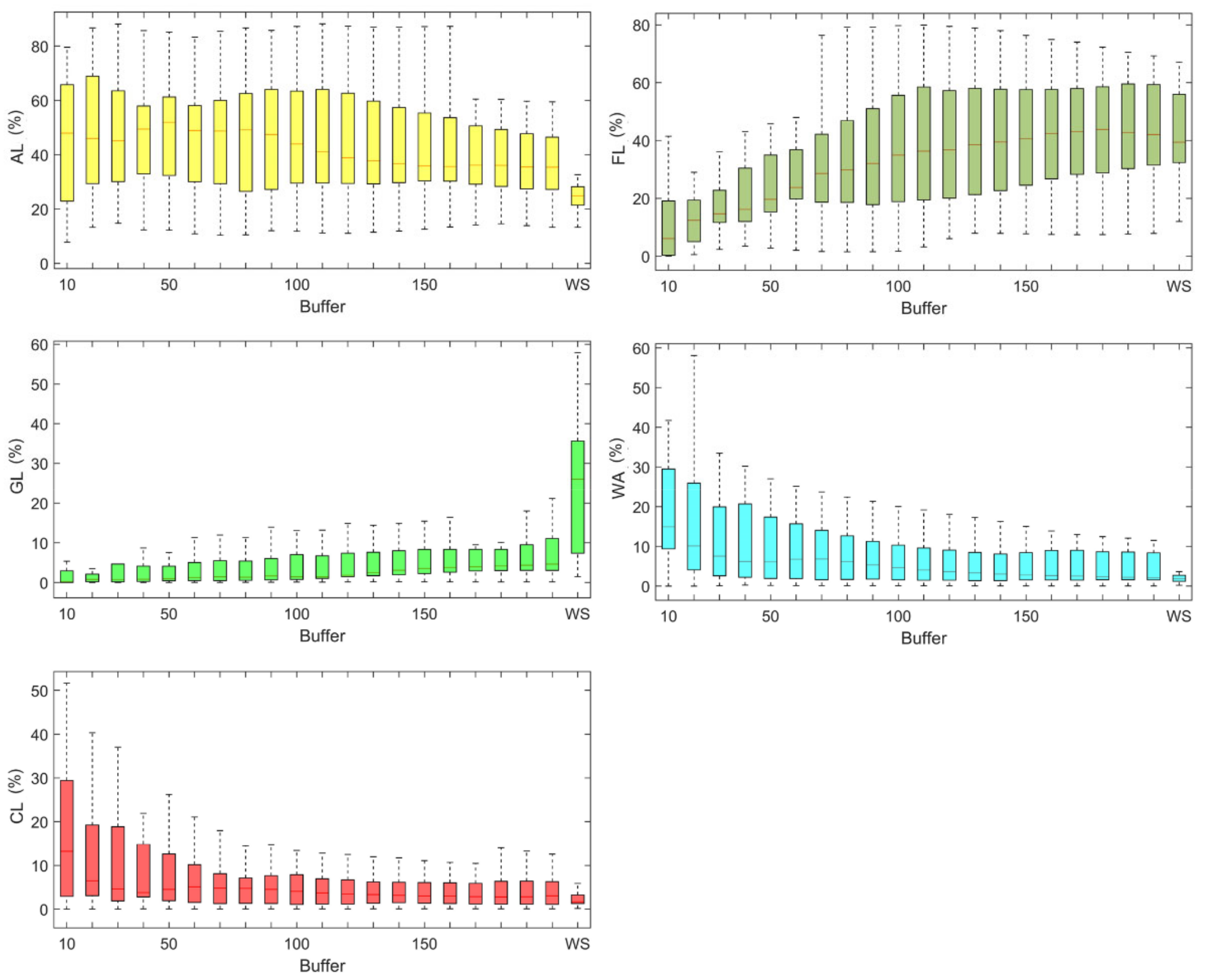
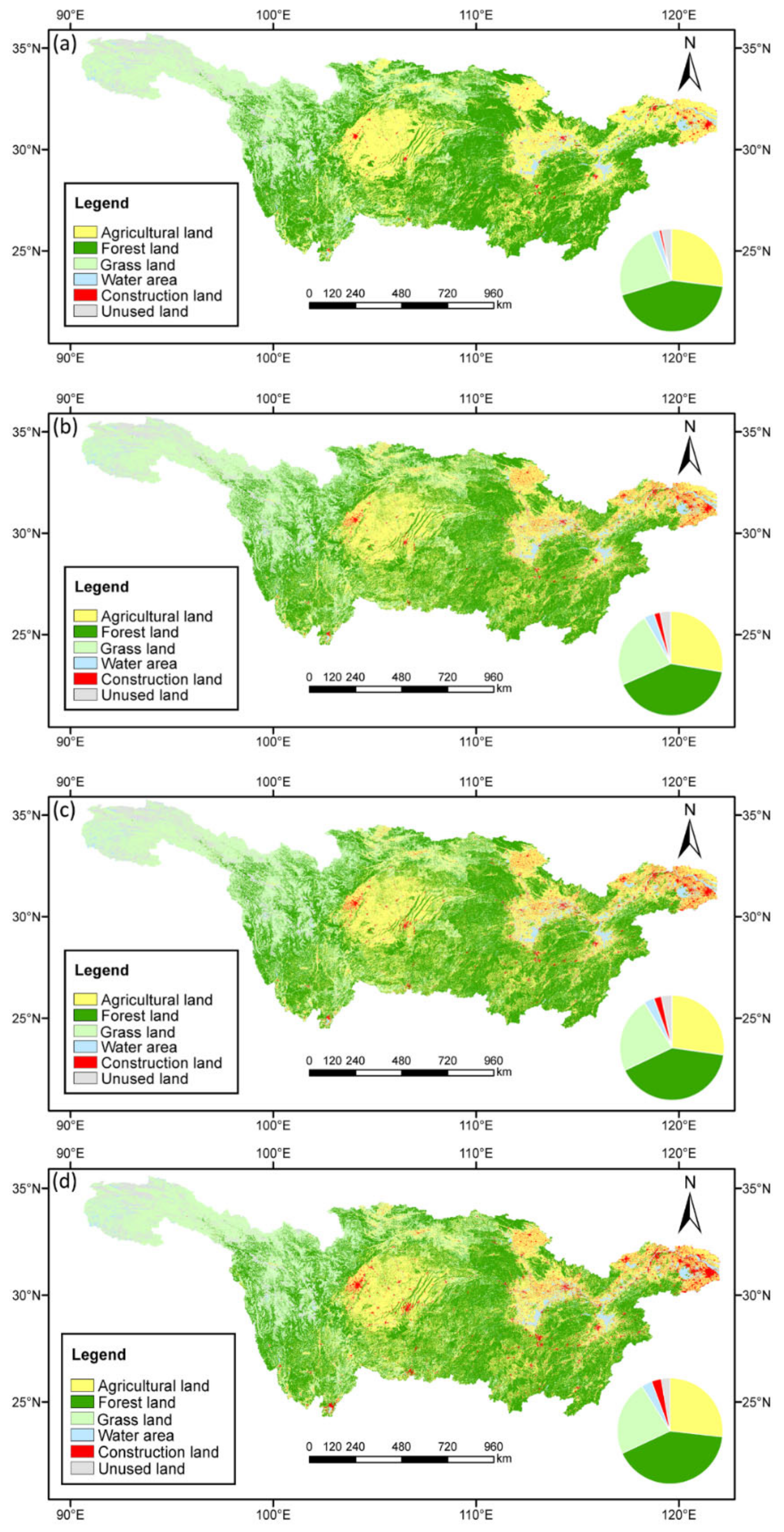
3.3. Land Use Change

As shown in Figure 8, the Yangtze River basin is mainly composed of FL, GL, and AL. AL is mainly distributed in the middle and lower reaches of rivers and around the Sichuan Basin. GL is mainly found in the upper reaches. FL is mainly distributed between GL and AL. CL is scattered in the Sichuan Basin and near the middle and lower reaches of the river. From 2005 to 2015, it is obvious that the CL expanded, and the CL was more densely distributed, especially in the middle and lower reaches, where urban expansion is obvious, replacing AL, resulting in the reduction in the AL area.

As can be seen from the line figure (Figure 9) and the table (

Table 3. Change in land use area proportion in different years in the Yangtze River basin. AP indicates the area proportion, and GR indicates the growth rate of the land use type from the previous year.

Land Use Type	Year
	2005		2010		2015		2018
	AP	GR	AP	GR	AP	GR	AP	GR
Agricultural land	26.91%	–	27.54%	2.28%	27.19%	−1.28%	26.76%	−1.52%
Forest land	43.48%	–	40.86%	−6.04%	40.75%	−0.28%	41.27%	1.32%
Grassland	23.32%	–	23.31%	−0.05%	23.31%	−0.03%	23.05%	−1.06%
Water area	2.42%	–	3.08%	26.95%	3.11%	1.18%	3.23%	3.78%
Construction land	0.81%	–	1.96%	143.03%	2.40%	22.47%	3.00%	25.16%
Unused land	3.06%	–	3.25%	5.98%	3.25%	−0.05%	2.68%	−17.43%

), the proportion of AL in the Yangtze River basin increased from 2005 to 2010 and decreased from 2010 to 2018. In addition, the major changes took place between 2005 and 2010. The proportion of FL in the whole basin showed a decreasing trend from 2005 to 2015, while it showed a small increasing trend from 2015 to 2018. The main changes also occurred from 2005 to 2010. The proportion of GL showed a downward trend from 2005 to 2015, while the change in trend was not obvious from 2005 to 2015. The main changes took place between 2015 and 2018. The proportion of WA showed an upward trend from 2005 to 2018, and the main change occurred from 2005 to 2010, with a 23.31% increase. The proportion of CL showed an upward trend from 2005 to 2015, and the main change occurred from 2005 to 2010, where the growth rate reached 143.03%. Although from 2010 to 2018, the growth rate showed a decrease, the growth rate was also high, reaching 20% at each stage.

Figure 10 shows the spatial distribution pattern of land use. With the increase in buffer size, the proportion of AL showed a trend of first increasing and then decreasing. With the increase in the buffer zone, the proportion of FL showed an upward trend. With the increase in the buffer zone, the percentage of GL showed an upward trend, and the increase was most significant from 200 km to the basin. With the increase in the buffer zone, the percentage of WA showed a decreasing trend and the percentage of CL showed a downward trend.

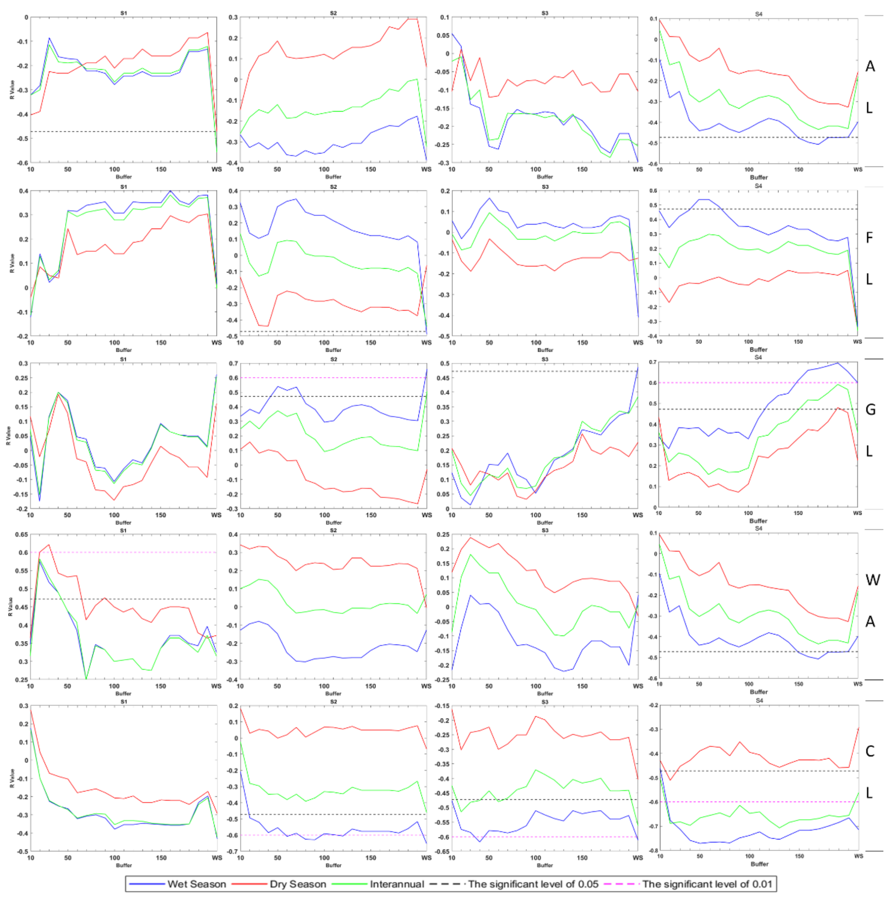
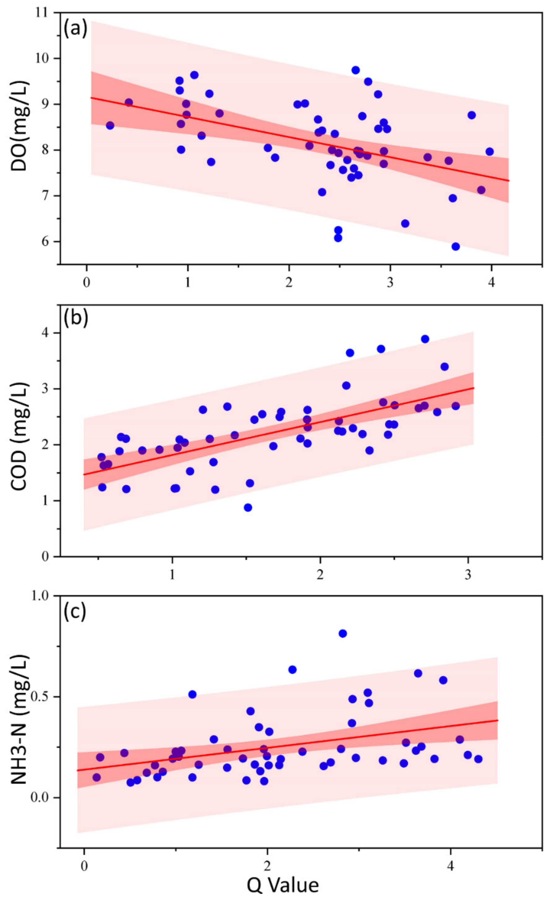
3.4. Correlation Analysis of Water Quality and Land Use

Water quality data from 2006 to 2018 were divided into four groups: S1, S2, S3, and S4. The specific grouping situation can be referred from Table 2. Spearman rank correlation analysis was used to analyze the correlation between the average values of different water quality pollutants (S1, S2, S3, S4) in interannual, wet, and dry seasons and the land use percentage in 2005, 2010, 2015, and 2018.

It can be seen from Figure 11, Figure 12 and Figure 13 that except for S1 and S4, the correlation between AL and DO touched the significance level of 0.05, and all other periods did not exceed the significance level of 0.05. Moreover, the correlation was higher in the wet season and consistent in the three stages, showing a negative correlation. In the dry season, there was only a negative correlation in S1, S3, and S4 and a positive correlation in S2. There was a positive correlation between AL, and COD_Mn and NH₃-N, and the correlation increased continuously from S1 to S4, and the degree of increase was greater from S1 to S2. At the same time, there was a certain seasonal change in the correlation, and the seasonal difference decreased gradually with the change in time; moreover, the correlation changed from the dry season to the wet season. The correlation between AL and pollutants also had a certain scale effect, showing a trend of first increasing and then decreasing. The correlation between AL and COD_Mn reached the maximum in the 110 km buffer in S1, the optimal buffer in S2 and S3 was 180 km, and S4 reached the maximum in the 170 km buffer. The correlation between AL and NH₃-N reached the maximum in the 90 km buffer in S1, 20 km buffer in S2, 70 km buffer in S3, and 20 km buffer in S4.

The correlation between FL and DO was low in all periods. There was a positive correlation in the wet season; a negative correlation in the dry season in S2, S3, and S4; and a positive correlation in S1. There was a negative correlation between FL, and COD_Mn and NH₃-N. In addition, the correlation between FL and NH₃-N increased greatly from S1 to S3 and decreased slightly from S3 to S4. The correlation between AL and COD_Mn increased from S1 to S4. The correlation between COD_Mn and FL showed a certain seasonal variation, and this seasonal difference gradually decreased with time. The correlation was higher in the dry season in S1 and higher in the wet season in S2 to S4. The correlation between NH₃-N and FL showed a higher correlation in the dry season in S1 and S2 and in the wet season in S3 and S4. In terms of the scale effect, the correlation between FL and COD_Mn increased first and then decreased with the increase in the buffer, reaching the maximum in the 80 km buffer of S1, 110 km buffer of S2, 180 km buffer of S3, and 170 km buffer of S4. The correlation between FL and NH₃-N decreased with the increase in the buffer area, reaching the maximum in the 50 km buffer of S1, 10 km buffer of S2, 70 km buffer of S3, and 20 km buffer of S4. When it comes to the watershed scale, the correlation was low.

The correlation between DO and GL was mainly positive, but some buffers in S1 and S2 were negatively correlated, and the correlation was high in the wet season and reached the maximum at the watershed scale. There was a negative correlation between GL, and COD_Mn and NH₃-N. The seasonal difference of correlation between GL and COD_Mn was greater in the dry season in S1 and S3 and greater in the wet season in S2 and S4, and the seasonal difference of correlation between grassland and NH₃-N was small. The scale effect of the correlation between GL and COD_Mn changed steadily in S1 but did not change much with the scale change. In S2 to S4, the correlation increased with the increase in buffer. At 200 km, the correlation was the largest but continued to increase to the basin scale, the correlation will decrease, and S3 had the largest correlation. The correlation between NH₃-N and grassland, with the increase in the buffer zone, formed two extreme points at 40 km, and 140–160 km.

The correlation between DO and WA showed a significant seasonal difference, showing a positive correlation in both S1 stages but a negative correlation in the wet season and a positive correlation in the dry season. There was a positive correlation between WA, and COD_Mn and NH₃-N, while there was a significant seasonal difference. The correlation between WA, and COD_Mn and NH₃-N was significantly higher in the dry season than in the wet season, and S2 had the highest correlation, while S1 had the lowest correlation. In terms of scale, the correlation with the two pollutants first increased and then decreased with the increase in the buffer zone. The maximum correlation between water and COD_Mn was 130–140 km in S1 to S4. The maximum correlation between water and NH₃-N was 60–70 km in S1 to S3 and 110 km in S4.

The correlation between DO and CL had the most obvious seasonal difference, and the correlation was not high in the S1 stage, but in S2 to S4, there was a significant negative correlation in the wet season, a lower correlation in the S2 dry season, and a non-significant negative correlation in the S1, S3, and S4 dry season. CL was positively correlated with COD_Mn and NH₃-N. The correlation between CL and COD_Mn showed an upward trend from S1 to S4, and the correlation reached a higher value with the increase in the buffer area. The correlation between CL and NH₃-N was the maximum in S1 and the minimum in S4. In S1 and S2, the correlation increased first and then became stable with the increase in the buffer size. The maximum correlation between CL and COD_Mn was 200 km in S1 to S4. The maximum correlation between CL and NH₃-N was 60 km in S1 to S2 and 80–90 km in S3 to S4.

Because the correlation in S1 was low, the correlation in S2 to S4 was more consistent, and S4 was the closest to the current stage, so we used the correlation in S4 to analyze the differences between different land types. As shown in

Table 4. Comparison of the maximum correlation and the buffer (S4) of land use and water quality in different seasons.

Land Use	Wet Season
	DO		CODMn		NH3-N
	Max. R	Buffer	Max. R	Buffer	Max. R	Buffer
AL	−0.51	17	0.83	17	0.56	2
FL	0.54	5	−0.63	14	−0.47	1
GL	0.69	19	−0.55	19	−0.7	3
WA	−0.45	13	0.28	14	0.36	7
CL	−0.77	5	0.7	20	0.37	6
Land Use	Dry Season
	DO		CODMn		NH3-N
	Max. R	Buffer	Max. R	Buffer	Max. R	Buffer
AL	−0.33	20	0.58	17	0.38	1
FL	−0.17	2	−0.63	4	−0.28	1
GL	0.48	19	−0.68	20	−0.68	3
WA	−0.22	13	0.62	14	0.26	7
CL	−0.51	2	0.76	13	0.31	6

, CL, AL, and WA had a negative impact on water quality. In any season, CL had a greater negative effect on DO than AL, and WA had the lowest negative effect. FL had a negative effect in the wet season, but the effect was low. In contrast, the negative effect on NH₃-N showed that AL was greater than CL in two seasons. Moreover, the negative effect on COD_Mn showed a difference in different seasons, indicating that the effect of AL is greater than that of CL in the wet season and CL affects more in the dry season.

4. Discussion

It can be seen from the spatiotemporal variation of water quality that the overall water quality in the Yangtze River basin is improving, and there are obvious seasonal and spatial differences. The level of DO and COD_Mn is poor in the wet season and good in the dry season. The level of NH₃-N is better in the dry season, but worse in the wet season. This is consistent with previous research results [42]. The main reason may be due to the high stream flow in the wet season when the concentration of DO and NH₃-N is diluted, while the precipitation and discharge are less in the dry season, the river self-purification capacity is low causing difficulty to the pollutant to spread. But COD_Mn are easily washed away by rainwater and runoff, which also leads to the increase of water quality pollution with the increase of runoff [24].

From 2005 to 2018, the land use change was mainly manifested as the increase in CL, AL increased from 2005 to 2010 and decreased after 2010, while FL decreased in a certain proportion from 2005 to 2010 but changed little after 2010. The GL appeared to be changing less. This result is mainly due to the influence of China’s policy of returning farmland to FL and GL, which effectively prevents the reduction in forestland and grassland. From 2005 to 2010, urbanization replaced a large amount of forestland, which led to the continuous reduction in FL and the continuous increase in CL. In terms of the spatial scale, AL, CL, and WA were mainly concentrated in a smaller buffer scale, while FL and GL were mainly concentrated in a larger buffer scale and even concentrated in the watershed scale. This may be because areas with small buffer zones are close to water sources and have sufficient water resources, which is conducive to economic and social development. At the same time, the soil near the river bank has high fertility and high productivity of vegetation, making it the first choice for residents to reclaim cultivated land.

In this paper, the relationship between water quality and land use is studied to reveal the relationship between them. Many previous studies have pointed out that vegetated areas make a positive contribution to water quality, whereas agricultural and built-up land uses make a negative contribution to water quality [26,28,43,44]. Our results are similar to those of previous studies. AL and CL are often associated with severe deterioration of surface water quality due to the discharge of household and industrial wastewater, livestock wastewater, rainstorm runoff, etc. [24]. CL can reflect human activities that produce a large amount of living and industrial wastewater, which flows into rivers with rainwater and runoff and affects the water quality of rivers. Agricultural production requires the application of large amounts of nitrogen fertilizer. Although nitrogen fertilizer can increase agricultural output, excessive application causes excess nitrogen and phosphorus elements to enter the water environment and cause water pollution [16]. Vegetated areas, including FL and GL, make a positive contribution to water quality, suggesting the fixation and absorption effects of pollutants and reducing the pollutants transported to the river through surface runoff [45].

Seasonal precipitation can affect water quality through flushing and dilution, leading to seasonal variations in pollutants [46]. During the wet season, NH₃-N and COD_Mn are easier to diffuse due to the flushing effect in less urbanized areas [47], which can explain the result that AL is more influential in the wet season. Moreover, due to unreasonable fertilization and irrigation before the wet season, AL also produces more pollution load during the wet season [48]. However, CL acts as a proxy for a point source, pollutants are mainly transported through pipes, and rainwater and runoff on the land surface do not diffuse pollution [49]. The main pollutant comes from domestic sewage, which is diluted during the wet season, thus reducing the impact of CL on water quality [50]. It can also be seen from our results that the correlation of CL with NH3-N and CODMn is mostly reflected in the characteristic of being higher in the dry season and lower in the wet season, which proves the rationality of our results. Previous studies have proved that the concentration of DO is higher at lower temperature [51]. In the wet season, not only does high temperature affect the concentration of DO but also more precipitation dilutes the concentration of DO, and the pollutants produced by Al and CL are more likely to lead to water eutrophication [52,53]. This can be reflected from the result that the effects of Al and CL on DO in the wet season are significantly greater than that in the dry season. Through multi-temporal and spatial scale studies, this paper found that the impact of land use on water quality is scale dependent, which has been confirmed in previous studies [13,23]. However, the opinions are contradictory. On the one hand, some scholars believe that the watershed scale can better explain the relationship between land use and water quality [9,54]. On the other hand, some scholars believe that the closer the land to the river bank, the higher the correlation between land use and water quality [55,56]. The research results of different land use types over many years show that the optimal research scales are different for different land use types, different spatial scales, and different seasons.

On the spatial scale, the correlation between COD_Mn and land use is larger than that between NH₃-N and land use in larger buffer zones, indicating that COD_Mn can affect water quality in a wider range than NH₃-N. The correlation between CL and COD_Mn increases with the increase in the buffer. This is mainly because urban drainage is usually directly discharged into sewage facilities and can be transported into rivers through long-distance transportation [24]. While the correlation between AL and COD_Mn does not increase continuously, it is also maintained at a high level in a large buffer. The reason may be that NH₃-N is more prone to retention in the soil [57], resulting in weaker migration of NH₃-N than that of COD_Mn. This also explains why the correlation between AL and NH₃-N decreases with the increase in the buffer.

To further reveal the legitimacy of our findings, we refer to Şandric et al.’s work [9], who classified and scored the threat levels of different land uses for water quality. According to our result, under the best buffer, the grid values of each land use are replaced by scores and the weighted average is calculated to a value Q, which can represent the threat level of land use. We divided the scores of each land use of DO and COD_Mn into the following: CL is a great threat (score 5), AL is a certain threat (score 3), WA is a minor threat (score 1), and FL and GL are no threat (score 0). The land use levels of NH₃-N were divided into AL (score 5), CL (score 3), WA (score 1), and FL and GL (score 0) according to the results of the correlation between water quality and land use. We drew a scatter plot for comparison between the calculated Q-value and each water quality index and calculated each Spearman correlation coefficient, as shown in Figure 14 and

Table 5. Relation between Q-value and water quality indexes.

Water Quality Indexes	Spearman R	p-Value
DO	−0.44	<0.01
CODMn	0.73	<0.01
NH3-N	0.46	<0.01

. From the scatter diagram, it can be seen that the R-value has a good fitting effect with water quality, and the effect of COD_Mn is the best. It can also be seen from the table that p-values are less than 0.01, indicating that the R-value has an obvious correlation with water quality, and the correlation of COD_Mn has reached more than 0.7. This result proves that it is reasonable for us to use the optimal buffer zone to identify the relationship between land use and water quality, and the results are persuasive.

Through the above comprehensive analysis, we get some useful conclusions. However, there are many factors affecting water quality, and other factors, such as slope and socio-economic factors, also affect water quality [58,59]. Per the conclusion of this paper, if the best buffer zone can be combined under different topographic conditions and integrated into different socio-economic scenarios, it may provide a better water quality assessment effect.

5. Conclusions

This paper discusses the changes in water quality and land use in the Yangtze River basin and discusses the relationship between water quality and land use from multiple temporal and spatial perspectives. The results show that all kinds of water quality mainly show up and down fluctuations or obvious downward trends, but different water quality categories in different regions reflect different trends. Water quality pollutants in tributaries are significantly higher than those in the main stream, and the concentration of pollutants increases with the decrease in the distance from the estuary. CL and AL have a negative effect on water quality, while FL and GL have a purifying effect on water quality. In particular, AL and CL have a significant positive correlation with pollutants in water. Moreover, their correlations have obvious seasonal differences, which mainly show that Al has a great impact on pollutants in the wet season, while CL has a great impact on pollutants in the dry season. Meanwhile, the correlation between different land use types and water quality is different at different spatial scales, showing that land use affects COD_Mn on a larger scale and NH₃-N on a smaller scale. This multi-scale spatio-temporal relationship between land use and water quality proves that the treatment of different pollutants should be carried out at different spatial and temporal scales of land planning. An understanding of the relationship between land use and water quality can improve science and land use policies, leading to better management of land use, and is important for the sustainable development of water ecosystems.

References

1. Reid, A.J.; Carlson, A.K.; Creed, I.F.; Eliason, E.J.; Gell, P.A.; Johnson, P.T.; Kidd, K.A.; MacCormack, T.J.; Olden, J.D.; Ormerod, S.J.; et al. Emergingthreats and persistent conservation challenges for fresh water biodiversity. Biol. Rev. 2019, 94, 849–873. [Google Scholar] [CrossRef] [PubMed] [Green Version]
2. Albert, J.S.; Destouni, G.; Duke-Sylvester, S.M.; Magurran, A.E.; Oberdorff, T.; Reis, R.E.; Winemiller, K.O.; Ripple, W.J. Scientists’ warning to humanity on the freshwater biodiversity crisis. Ambio 2021, 50, 85–94. [Google Scholar] [CrossRef] [PubMed]
3. Moore, J.W. Bidirectional connectivity in rivers and implications for watershed stability and management. Can. J. Fish. Aquat. Sci. 2015, 72, 785–795. [Google Scholar] [CrossRef] [Green Version]
4. Song, Y.; Song, X.; Shao, G.; Hu, T. Effects of Land Use on Stream Water Quality in the Rapidly Urbanized Areas: A Multiscale Analysis. Water 2020, 12, 1123. [Google Scholar] [CrossRef] [Green Version]
5. Shabani, A.; Woznicki, S.A.; Mehaffey, M.; Butcher, J.; Wool, T.A.; Whung, P.-Y. A coupled hydrodynamic (HEC-RAS 2D) and water quality model (WASP) for simulating flood-induced soil, sediment, and contaminant transport. J. Flood Risk Manag. 2021, e12747. [Google Scholar] [CrossRef]
6. Wang, J.; Fu, Z.; Qiao, H.; Liu, F. Assessment of eutrophication and water quality in the estuarine area of Lake Wuli, Lake Taihu, China. Sci. Total Environ. 2019, 650, 1392–1402. [Google Scholar] [CrossRef]
7. Chrobak, G.; Kowalczyk, T.; Fischer, T.B.; Szewrański, S.; Chrobak, K.; Kazak, J.K. Ecological state evaluation of lake ecosystems revisited: Latent variables with kSVM algorithm approach for assessment automatization and data comprehension. Ecol. Indic. 2021, 125, 107567. [Google Scholar] [CrossRef]
8. Li, J.; Tian, L.; Wang, Y.; Jin, S.; Li, T.; Hou, X. Optimal sampling strategy of water quality monitoring at high dynamic lakes: A remote sensing and spatial simulated annealing integrated approach. Sci. Total Environ. 2021, 777, 146113. [Google Scholar] [CrossRef]
9. Şandric, I.; Satmari, A.; Zaharia, C.; Petrovici, M.; Cîmpean, M.; Battes, K.-P.; David, D.-C.; Pacioglu, O.; Weiperth, A.; Gál, B.; et al. Integrating catchment land cover data to remotely assess freshwater quality: A step forward in heterogeneity analysis of river networks. Aquat. Sci. 2019, 81, 26. [Google Scholar] [CrossRef]
10. Ahearn, D.S.; Sheibley, R.W.; Dahlgren, R.A.; Anderson, M.; Johnson, J.; Tate, K.W. Land use and land cover influence on water quality in the last free-flowing river draining the western Sierra Nevada, California. J. Hydrol. 2005, 313, 234–247. [Google Scholar] [CrossRef]
11. Rodrigues, V.; Estrany, J.; Ranzini, M.; Cicco, V.; de Martín-Benito, J.M.T.; Hedo, J.; Lucas-Borja, M.E. Effects of land use and seasonality on stream water quality in a small tropical catchment: The headwater of Córrego Água Limpa, São Paulo (Brazil). Sci. Total Environ. 2018, 622–623, 1553–1561. [Google Scholar] [CrossRef] [PubMed] [Green Version]
12. Huang, J.; Li, Q.; Pontius, R.G.; Klemas, V.; Hong, H. Detecting the dynamic linkage between landscape characteristics and water quality in a subtropical coastal watershed, Southeast China. Environ. Manag. 2013, 51, 32–44. [Google Scholar] [CrossRef] [PubMed]
13. Park, S.-R.; Lee, S.-W. Spatially Varying and Scale-Dependent Relationships of Land Use Types with Stream Water Quality. Int. J. Environ. Res. Public Health 2020, 17, 1673. [Google Scholar] [CrossRef] [Green Version]
14. Kronvang, B.; Wendland, F.; Kovar, K.; Fraters, D. Land Use and Water Quality. Water 2020, 12, 2412. [Google Scholar] [CrossRef]
15. Shi, P.; Zhang, Y.; Song, J.; Li, P.; Wang, Y.; Zhang, X.; Li, Z.; Bi, Z.; Zhang, X.; Qin, Y.; et al. Response of nitrogen pollution in surface water to land use and social-economic factors in the Weihe River watershed, northwest China. Sustain. Cities Soc. 2019, 50, 101658. [Google Scholar] [CrossRef]
16. Zhang, S.; Hou, X.; Wu, C.; Zhang, C. Impacts of climate and planting structure changes on watershed runoff and nitrogen and phosphorus loss. Sci. Total Environ. 2020, 706, 134489. [Google Scholar] [CrossRef]
17. Li, S.; Peng, S.; Jin, B.; Zhou, J.; Li, Y. Multi-scale relationship between land use/land cover types and water quality in different pollution source areas in Fuxian Lake Basin. PeerJ 2019, 7, e7283. [Google Scholar] [CrossRef] [Green Version]
18. Rodríguez-Romero, A.; Rico-Sánchez, A.; Mendoza-Martínez, E.; Gómez-Ruiz, A.; Sedeño-Díaz, J.; López-López, E. Impact of Changes of Land Use on Water Quality, from Tropical Forest to Anthropogenic Occupation: A Multivariate Approach. Water 2018, 10, 1518. [Google Scholar] [CrossRef] [Green Version]
19. Pratt, B.; Chang, H. Effects of land cover, topography, and built structure on seasonal water quality at multiple spatial scales. J. Hazard. Mater. 2012, 209–210, 48–58. [Google Scholar] [CrossRef]
20. Nelson Mwaijengo, G.; Msigwa, A.; Njau, K.N.; Brendonck, L.; Vanschoenwinkel, B. Where does land use matter most? Contrasting land use effects on river quality at different spatial scales. Sci. Total Environ. 2020, 715, 134825. [Google Scholar] [CrossRef]
21. Zorzal-Almeida, S.; Salim, A.; Andrade, M.R.M.; Nascimento, M.d.N.; Bini, L.M.; Bicudo, D.C. Effects of land use and spatial processes in water and surface sediment of tropical reservoirs at local and regional scales. Sci. Total Environ. 2018, 644, 237–246. [Google Scholar] [CrossRef]
22. Wu, J.; Lu, J. Spatial scale effects of landscape metrics on stream water quality and their seasonal changes. Water Res. 2021, 191, 116811. [Google Scholar] [CrossRef] [PubMed]
23. Ding, J.; Jiang, Y.; Liu, Q.; Hou, Z.; Liao, J.; Fu, L.; Peng, Q. Influences of the land use pattern on water quality in low-order streams of the Dongjiang River basin, China: A multi-scale analysis. Sci. Total Environ. 2016, 551–552, 205–216. [Google Scholar] [CrossRef]
24. Liu, J.; Zhang, X.; Wu, B.; Pan, G.; Xu, J.; Wu, S. Spatial scale and seasonal dependence of land use impacts on riverine water quality in the Huai River basin, China. Environ. Sci. Pollut. Res. Int. 2017, 24, 20995–21010. [Google Scholar] [CrossRef] [PubMed]
25. Zhang, Y.; Li, P.; Liu, X.; Xiao, L.; Shi, P.; Zhao, B. Effects of farmland conversion on the stoichiometry of carbon, nitrogen, and phosphorus in soil aggregates on the Loess Plateau of China. Geoderma 2019, 351, 188–196. [Google Scholar] [CrossRef]
26. Shi, P.; Zhang, Y.; Li, Z.; Li, P.; Xu, G. Influence of land use and land cover patterns on seasonal water quality at multi-spatial scales. Catena 2017, 151, 182–190. [Google Scholar] [CrossRef]
27. Li, G.Y.; Li, L.Z.; Kong, M. Multiple-Scale Analysis of Water Quality Variations and Their Correlation with Land use in Highly Urbanized Taihu Basin, China. Bull. Environ. Contam. Toxicol. 2021, 106, 218–224. [Google Scholar] [CrossRef]
28. Zhang, J.; Li, S.; Dong, R.; Jiang, C.; Ni, M. Influences of land use metrics at multi-spatial scales on seasonal water quality: A case study of river systems in the Three Gorges Reservoir Area, China. J. Clean. Prod. 2019, 206, 76–85. [Google Scholar] [CrossRef]
29. Li, S.; Gu, S.; Tan, X.; Zhang, Q. Water quality in the upper Han River basin, China: The impacts of land use/land cover in riparian buffer zone. J. Hazard. Mater. 2009, 165, 317–324. [Google Scholar] [CrossRef]
30. Zhao, J.; Lin, L.; Yang, K.; Liu, Q.; Qian, G. Influences of land use on water quality in a reticular river network area: A case study in Shanghai, China. Landsc. Urban. Plan. 2015, 137, 20–29. [Google Scholar] [CrossRef]
31. Xu, J.; Liu, R.; Ni, M.; Zhang, J.; Ji, Q.; Xiao, Z. Seasonal variations of water quality response to land use metrics at multi-spatial scales in the Yangtze River basin. Environ. Sci. Pollut. Res. Int. 2021. [Google Scholar] [CrossRef]
32. Li, X.; Xu, Y.; Li, M.; Ji, R.; Dolf, R.; Gu, X. Water Quality Analysis of the Yangtze and the Rhine River: A Comparative Study Based on Monitoring Data from 2007 to 2018. Bull. Environ. Contam. Toxicol. 2021, 106, 825–831. [Google Scholar] [CrossRef] [PubMed]
33. Chen, T.; Wang, Y.; Gardner, C.; Wu, F. Threats and protection policies of the aquatic biodiversity in the Yangtze River. J. Nat. Conserv. 2020, 58, 125931. [Google Scholar] [CrossRef]
34. Zhong, Y.; Lin, A.; He, L.; Zhou, Z.; Yuan, M. Spatiotemporal Dynamics and Driving Forces of Urban Land-Use Expansion: A Case Study of the Yangtze River Economic Belt, China. Remote Sens. 2020, 12, 287. [Google Scholar] [CrossRef] [Green Version]
35. Duan, W.; He, B.; Chen, Y.; Zou, S.; Wang, Y.; Nover, D.; Chen, W.; Yang, G. Identification of long-term trends and seasonality in high-frequency water quality data from the Yangtze River basin, China. PLoS ONE 2018, 13, e0188889. [Google Scholar] [CrossRef] [PubMed]
36. Sun, J.; Ding, L.; Li, J.; Qian, H.; Huang, M.; Xu, N. Monitoring Temporal Change of River Islands in the Yangtze River by Remotely Sensed Data. Water 2018, 10, 1484. [Google Scholar] [CrossRef] [Green Version]
37. Ma, X.; Wang, L.; Yang, H.; Li, N.; Gong, C. Spatiotemporal Analysis of Water Quality Using Multivariate Statistical Techniques and the Water Quality Identification Index for the Qinhuai River Basin, East China. Water 2020, 12, 2764. [Google Scholar] [CrossRef]
38. Mann, H.B. Nonparametric Tests against Trend. Econometrica 1945, 13, 245. [Google Scholar] [CrossRef]
39. Kendall, M.G. Rank Correlation Methods. Biometrika 1957, 44, 298. [Google Scholar] [CrossRef]
40. Wei, X.; Wang, N.; Luo, P.; Yang, J.; Zhang, J.; Lin, K. Spatiotemporal Assessment of Land Marketization and Its Driving Forces for Sustainable Urban–Rural Development in Shaanxi Province in China. Sustainability 2021, 13, 7755. [Google Scholar] [CrossRef]
41. Zar, J.H. Spearman Rank Correlation. In Encyclopedia of Biostatistics; Armitage, P., Colton, T., Eds.; John Wiley & Sons, Ltd.: Chichester, UK, 2005; ISBN 047084907X. [Google Scholar]
42. Huang, L.; Zhong, M.; Gan, Q.; Liu, Y. A Novel Calendar-Based Method for Visualizing Water Quality Change: The Case of the Yangtze River 2006–2015. Water 2017, 9, 708. [Google Scholar] [CrossRef] [Green Version]
43. Wan, R.; Cai, S.; Li, H.; Yang, G.; Li, Z.; Nie, X. Inferring land use and land cover impact on stream water quality using a Bayesian hierarchical modeling approach in the Xitiaoxi River Watershed, China. J. Environ. Manag. 2014, 133, 1–11. [Google Scholar] [CrossRef] [PubMed]
44. Bu, H.; Meng, W.; Zhang, Y.; Wan, J. Relationships between land use patterns and water quality in the Taizi River basin, China. Ecol. Indic. 2014, 41, 187–197. [Google Scholar] [CrossRef]
45. Piatek, K.B.; Christopher, S.F.; Mitchell, M.J. Spatial and temporal dynamics of stream chemistry in a forested watershed. Hydrol. Earth Syst. Sci. 2009, 13, 423–439. [Google Scholar] [CrossRef] [Green Version]
46. Park, J.-H.; Inam, E.; Abdullah, M.H.; Agustiyani, D.; Duan, L.; Hoang, T.T.; Kim, K.-W.; Kim, S.D.; Nguyen, M.H.; Pekthong, T.; et al. Implications of rainfall variability for seasonality and climate-induced risks concerning surface water quality in East Asia. J. Hydrol. 2011, 400, 323–332. [Google Scholar] [CrossRef]
47. Zhou, P.; Huang, J.; Pontius, R.G.; Hong, H. New insight into the correlations between land use and water quality in a coastal watershed of China: Does point source pollution weaken it? Sci. Total Environ. 2016, 543, 591–600. [Google Scholar] [CrossRef] [PubMed]
48. Wang, H.; He, P.; Shen, C.; Wu, Z. Effect of irrigation amount and fertilization on agriculture non-point source pollution in the paddy field. Environ. Sci. Pollut. Res. Int. 2019, 26, 10363–10373. [Google Scholar] [CrossRef]
49. Guo, W.; Fu, Y.; Ruan, B.; Ge, H.; Zhao, N. Agricultural non-point source pollution in the Yongding River Basin. Ecol. Indic. 2014, 36, 254–261. [Google Scholar] [CrossRef]
50. Bilgin, A.; Bayraktar, H.D. Assessment of lake water quality using multivariate statistical techniques and chlorophyll-nutrient relationships: A case study of the Göksu Lake. Arab. J. Geosci. 2021, 14, 1–13. [Google Scholar] [CrossRef]
51. Harvey, R.; Lye, L.; Khan, A.; Paterson, R. The Influence of Air Temperature on Water Temperature and the Concentration of Dissolved Oxygen in Newfoundland Rivers. Can. Water Resour. J. 2011, 36, 171–192. [Google Scholar] [CrossRef]
52. Uriarte, M.; Yackulic, C.B.; Lim, Y.; Arce-Nazario, J.A. Influence of land use on water quality in a tropical landscape: A multi-scale analysis. Landsc. Ecol. 2011, 26, 1151–1164. [Google Scholar] [CrossRef] [Green Version]
53. Zhang, Y.; Luo, P.; Zhao, S.; Kang, S.; Wang, P.; Zhou, M.; Lyu, J. Control and remediation methods for eutrophic lakes in the past 30 years. Water Sci. Technol. 2020, 81, 1099–1113. [Google Scholar] [CrossRef]
54. Nash, M.S.; Heggem, D.T.; Ebert, D.; Wade, T.G.; Hall, R.K. Multi-scale landscape factors influencing stream water quality in the state of Oregon. Environ. Monit. Assess. 2009, 156, 343–360. [Google Scholar] [CrossRef] [PubMed]
55. Miserendino, M.L.; Casaux, R.; Archangelsky, M.; Di Prinzio, C.Y.; Brand, C.; Kutschker, A.M. Assessing land-use effects on water quality, in-stream habitat, riparian ecosystems and biodiversity in Patagonian northwest streams. Sci. Total Environ. 2011, 409, 612–624. [Google Scholar] [CrossRef] [PubMed]
56. Fernandes, J.D.F.; de Souza, A.L.T.; Tanaka, M.O. Can the structure of a riparian forest remnant influence stream water quality? A tropical case study. Hydrobiologia 2014, 724, 175–185. [Google Scholar] [CrossRef]
57. Xie, D.; Duan, L.; Si, G.; Liu, W.; Zhang, T.; Mulder, J. Long-Term 15 N Balance After Single-Dose Input of 15 N-Labeled NH 4+ and NO3 in a Subtropical Forest Under Reducing N Deposition. Glob. Biogeochem. Cycles 2021, 35, e2021GB006959. [Google Scholar] [CrossRef]
58. Fang, H. Effect of soil conservation measures and slope on runoff, soil, TN, and TP losses from cultivated lands in northern China. Ecol. Indic. 2021, 126, 107677. [Google Scholar] [CrossRef]
59. Li, H.; Jiang, Z.; Dong, G.; Wang, L.; Huang, X.; Gu, X.; Guo, Y. Spatiotemporal Coupling Coordination Analysis of Social Economy and Resource Environment of Central Cities in the Yellow River Basin. Discret. Dyn. Nat. Soc. 2021, 2021, 1–13. [Google Scholar] [CrossRef]
Figure 1. The location of water quality stations in the study area.
Remotesensing 13 03309 g001
Figure 2. Diagram of watershed (a) division and buffer zone (b) division in the Yangtze River basin (c) (taking Longdong Station as an example).
Remotesensing 13 03309 g002
Figure 3. Box plots of water quality concentration of DO (a) CODMn (b), and NH3-N (c) in the wet and dry seasons. The X-axis represents water quality stations, and the positive directions along the X-axis indicate an increase in the distance from the site to the estuary. The left side of the green line is the main stream, and the right side is the tributary.
Remotesensing 13 03309 g003
Figure 4. The monthly identification index of DO of each monitoring section (white block indicates lack of monitoring data). The first seven sites are the trunk streams.
Remotesensing 13 03309 g004
Figure 5. The monthly identification index of CODMn of each monitoring section (white block indicates lack of monitoring data). The first seven sites are the trunk streams.
Remotesensing 13 03309 g005
Figure 6. The monthly identification index of NH3-N of each monitoring section (white block indicates lack of monitoring data). The first seven sites are the trunk streams.
Remotesensing 13 03309 g006
Figure 7. Annual changes in water quality identification indexes of different pollutants. The first seven sites are the trunk streams.
Remotesensing 13 03309 g007
Figure 8. Changing trend in the identification index of comprehensive water quality. The blue line represents a significance level of 0.05, and the red line represents a significance level of 0.01.
Remotesensing 13 03309 g008
Figure 9. Land use distribution in 2005 (a), 2010 (b), 2015 (c), and 2018 (d).
Remotesensing 13 03309 g009
Figure 10. Box plot of 18 sites with different land use ratios in each buffer zone in 2018.
Remotesensing 13 03309 g010
Figure 11. Correlation index of DO and different land use types in different seasons in S1, S2, S3, and S4. Each row from the top to the bottom represents a type of land use.
Remotesensing 13 03309 g011
Figure 12. Correlation index of CODMN and different land use types in different seasons in S1, S2, and S3. Each row from the top to the bottom represents a type of land use.
Remotesensing 13 03309 g012
Figure 13. Correlation index of NH3-N and different land use types in different seasons in S1, S2, and S3. Each row from the top to the bottom represents a type of land use.
Remotesensing 13 03309 g013
Figure 14. Scatter plot of DO (a), CODMn (b), NH3-N (c) concentration, and Q-value. The red line is a linear fitting line. The dark-red shaded area is the 95% confidence interval, and the light-red shaded area is the 95% prediction interval.
Remotesensing 13 03309 g014