Abstract
The direct and indirect radiation forcing of aerosol particles deeply affect the energy budget and the atmospheric chemical and physical processes. To retrieve the vertical aerosol mass fluxes and to investigate the vertical transport process of aerosol by a coherent Doppler lidar (CDL), a practical method for instrumental calibration and aerosol optical properties retrieval based on CDL and sun photometer synchronization observations has been developed. A conversion of aerosol optical properties to aerosol microphysical properties is achieved by applying a well-developed algorithm. Furthermore, combining the vertical velocity measured simultaneously with a CDL, we use the eddy covariance (EC) method to retrieve the vertical turbulent aerosol mass fluxes by a CDL and sun photometer with a spatial resolution of 15 m and a temporal resolution of 1 s throughout the planetary boundary layer (PBL). In this paper, we present a measurement case of 24-h continuous fluxes observations and analyze the diurnal variation of the vertical velocity, the aerosol backscatter coefficient at 1550 nm, the mean aerosol mass concentration, and the vertical aerosol mass fluxes on 13 April 2020. Finally, the main relative errors in aerosol mass flux retrieval, including sample error , aerosol optical properties retrieval error , and error introduced from aerosol microphysical properties retrieval algorithm , are evaluated. The sample error is the dominating error which increases with height except during 12:00–13:12 LST. The aerosol optical properties retrieval error is 21% and the error introduced from the aerosol microphysical properties retrieval algorithm is less than 50%.
1. Introduction
The vertical transport of substance and energy has a significant effect on weather and climate change, especially in the planetary boundary layer (PBL), which is considered as the interface between the Earths’ surface and the free atmosphere. The vertical exchange of heat, water vapor, aerosol, trace gas, and other variables are all of great interest in recent years. Among that, although taking a small proportion in the atmosphere, aerosol particles strongly influence the climate and weather by affecting the energy budget and latent heating distribution [1]. Additionally, the distribution of aerosols significantly affect the energy transport in the atmosphere and the ocean below. Hence, it is important to make vertically resolved observations of aerosols, especially in the PBL. However, the aerosol’s contribution is still regarded as one of the largest uncertainties in estimation and evaluation of the Earth’s transport of radiant energy because of its variable amounts and properties in time and space [1].
For the turbulent flux detection, an ultrasonic anemometer and a fast-response transducer are frequently used to make in-situ measurements [2,3,4,5,6,7]. Networks aiming at the global fluxes observations, such as FLUXNET (https://daac.ornl.gov/FLUXNET, last accessed on 20 April 2021), have been established to achieve substance and energy exchange researches using the eddy covariance (EC) method which provides the fluxes of scalars contain CO2, CH4, water vapor, and heat fluxes with high temporal resolution [8]. However, in-situ flux measurements at single points could be derived which are frequently used to describe the transport process of relatively small scope.
With the development of the remote sensing instruments, especially the lidar which has obvious advantages including its high temporal and spatial resolution, high accuracy, a capability of large-scale profile observation [9], and so on, researches on the flux measurements by multi-types lidars in recent years have been widely conducted. Gal-Chen et al. (1992) retrieved the vertical fluxes of horizontal momentum and other turbulence parameters with a CO2 Doppler lidar [10]. Recently, researchers started to measure the momentum fluxes by different types of Doppler lidars with multiple scanning modes. Mann et al. (2010) used a continuous wave Doppler lidar and a pulsed Doppler lidar to measure the vertical fluxes of horizontal momentum. The results of momentum fluxes were compared with the sonic anemometer measurements at different heights and they showed good agreement [11]. Smalikho et al. (2017) retrieved the momentum fluxes and other turbulence parameters by a pulsed coherent Doppler lidar (PCDL) with the conical scanning mode. They also showed good agreement with sonic anemometer results. Additionally, applicability of this method and accuracy of turbulence parameters estimation were evaluated [12]. In general, momentum flux measurements can be individually conducted by a Doppler lidar while the heat fluxes and other substance fluxes are observed with Doppler lidar and other types of lidars. For heat flux, it was demonstrated earlier that the latent heat fluxes were estimated based on the Monin–Obukhov similarity theory [13] with a scanning Raman lidar [14]. In the subsequent researches, the profiles of sensible heat fluxes and latent heat fluxes were retrieved by a combination of a rotational Raman lidar, a water vapor differential absorption lidar (DIAL), and a Doppler wind lidar [15,16]. It was shown that, for a typical sensible heat flux profile, values are positive in the lower and middle convective boundary layer (CBL), while values are negative in the upper CBL and the lower free atmosphere [15]. Besides, some substance flux measurements have been achieved, such as the water vapor fluxes, which are usually obtained by a combination of water vapor DIAL and Doppler lidar [17,18,19,20,21], the CO2 fluxes observed with a coherent differential absorption lidar (CDIAL) earlier [22] and those measured in volcanic plumes [23,24] more recently, the ozone fluxes retrieved by a combination of an ozone DIAL and a Doppler lidar with a resolution of 120 m and 30 s [25], and the atomic mercury fluxes measured with a DIAL and a Doppler lidar [26].
As for the lidar observation of aerosol fluxes, it becomes more difficult due to the aerosol particles’ volatile composition and complicated properties, especially its variable hygroscopic growth. It means that the vertical transport of aerosol particles is associated with water uptake because of its different hygroscopic growth factors for updrafts and downdrafts [9]. Engelmann et al. (2008) reported lidar observations of the vertical aerosol mass flux by a multi-wavelength Raman lidar and a Doppler wind lidar with a spatial and temporal resolution of 75 m and 5 s. The aerosol optical properties were retrieved with the Raman lidar technique, and aerosol microphysical properties were obtained by applying a well-developed inversion algorithm introduced in Müller et al. (1999) [27]. The vertical aerosol mass fluxes with 0.5–2.5 were presented in the upper CBL and the relative errors of the aerosol mass flux retrieval were evaluated and quantified [9]. Chouza et al. (2016) conducted the wind and aerosol measurements simultaneously and investigated the Saharan dust long-range transport with an airborne Doppler wind lidar. For validation, they compared the results with the Monitoring Atmospheric Composition and Climate (MACC) model and analyzed the long-range transport characteristics of three regions [28]. With the similar technique that Engelmann et al. (2008) introduced, the PM2.5 mass concentrations and regional transport fluxes of different pollution levels were retrieved based on the vehicle-based mobile lidar observation and the Weather Research and Forecasting (WRF) model in Beijing [29]. In this study, a mobile lidar was used to measure the distribution and transport of PM2.5 while wind profiles were provided from the WRF model. It should be emphasized that, when the relative humidity (RH) is larger than 90%, the aerosol hygroscopic growth effect could not be ignored any more. Then, transportations of PM2.5 at the boundary of Beijing and Baoding on the southwest pathway were investigated in the winter of 2017 [30]. They found that the value of PM2.5 fluxes from Baoding to Beijing were positive when the southern wind appeared and that they were negative when the northern wind occurred below 500 m. Besides, the transport characteristics of PM2.5 of other regions such as Shenzhen were analyzed by a four-dimensional flux method and PM2.5 source contribution was identified accordingly [31]. In summary, to retrieve aerosol flux and investigate the aerosol transport process, it is frequently used to combine an aerosol lidar with a Doppler wind lidar or other numerical models. If the retrieval of aerosol fluxes could be realized by Doppler wind lidar individually, observation costs will be significantly reduced. Furthermore, because of its miniaturization and portability, it is promising to mount it on many mobile platforms such as a research vessel, a buoy, or an aircraft, so that large space-range observation will become possible.
In this paper, we briefly introduce a practical method to retrieve multi-wavelength aerosol optical properties based on a coherent Doppler lidar (CDL) and a sun photometer joint observation. By applying the well-developed aerosol microphysical properties inversion algorithm and assuming a typical particle density, the aerosol mass concentration is calculated and the vertical aerosol mass flux profiles could be derived with the EC method when the vertical velocities were obtained simultaneously. Additionally, a case study of a 24-h vertical aerosol mass fluxes observation is presented. The diurnal variation processes of the vertical velocity, the aerosol backscatter coefficient at 1550 nm, the mean aerosol mass concentration, and the vertical aerosol mass fluxes are analyzed, and the main relative errors involved are evaluated.
The paper is organized as follows. The description of the involved instruments, the retrieval method for the aerosol optical properties, and the vertical turbulent aerosol mass fluxes are provided in Section 2. Section 3 introduces the details of field experiments and one case study of a 24-h vertical aerosol mass fluxes observation. Section 4 summarizes the conclusions and the outlook of future studies.
2. Instruments and Methodology
2.1. Instruments
For the wind field observations, the CDL of type Wind3D 6000, which is jointed developed by Ocean University of China (OUC) and Qingdao Leice Transient Technology Co., Ltd., was applied. The specifications and schematic diagram of the CDL have been introduced in detail elsewhere [32,33,34]. For the aerosol optical properties retrieval, the simultaneous observations with a sun photometer and a CDL were performed. A sun photometer of the type CIMEL-318 was used to provide the aerosol optical depth (AOD) and Ångström exponent at the wavelengths of 440 nm, 670 nm, 870 nm, and 1020 nm. Thus, the aerosol size distributions could be estimated roughly [35] which act as a means of validation to evaluate the results of aerosol microphysical properties retrieved by CDL data. Besides, different lidar ratios could be set according to empirical values that were reported from other literatures [36].
2.2. Methodology
2.2.1. Wind Field Retrieval by a CDL
The CDL emits a 1550 nm laser beam into the atmosphere and receives the aerosol backscatter signal which carries the Doppler shift information. The radial velocity along the laser beam could then be obtained by Equation (1):
where is the Doppler frequency shift, is the radial velocity, and is the wavelength at 1550 nm. In the flux observation experiments, the vertical pointing mode was set and the vertical velocity could be retrieved directly with a range resolution of 15 m and a temporal resolution of 1 s. The velocity measurement uncertainty was less than 0.1 m/s [32].
2.2.2. Aerosol Optical Properties Retrieval by a CDL and a Sun Photometer
By combined observations of the CDL and the sun photometer, the integrated backscatter signal of the CDL could be calibrated with fitted AOD at 1550 nm from sun photometer measurements. This calibration method was introduced in a separate paper [37]. To verify the accuracy and applicability of this method, three validation experiments were conducted in 2019 and 2020. By applying the procedure that the reference mentioned above demonstrated to the processing of validation measurements datasets, good agreement between AOD from the CDL and AOD from the sun photometer with the correlation of 0.96, the RMSE of 0.0085, and the mean relative error of 21% was found of all the low-depolarization aerosol load days. Hence, it is proved that the retrieval of aerosol optical properties based on a calibrated CDL is feasible and reliable. It should be emphasized that this method is not applicable when the depolarization ratio of atmospheric aerosol load is too high (e.g., dust and volcanic ash aerosols with depolarization ratios larger than 0.1) and while the polarization-sensitive CDL is in use [37].
2.2.3. Vertical Aerosol Mass Fluxes Retrieval by a CDL and a Sun Photometer
Similarly, backscatter coefficients and extinction coefficients at the wavelengths of 440 nm, 670 nm, 870 nm, and 1020 nm could be retrieved with similar procedure given by Dai et al. (2021) [37]. The Equation (9) from Dai et al. (2021) is converted to the following equation:
where , and are wavelength conversion coefficients which could be estimated based on sun photometer measurements with Equation (3):
By inputting aerosol optical properties mentioned above and applying regularization inversion method [27], the particle volume concentration distribution could be calculated. After integrating and multiplying an assuming typical particle density which was set as 1.6 referring to previous studies [9,38], the particle mass concentration could be estimated. It should be noticed that the assumed aerosol density needs to be adjusted carefully, according to the empirical values that Ma et al. (2020) reported [39]. According to the statistical analysis of many researches, the assumed aerosol density of 1.6 g/cm3 is appropriate and acceptable for most atmospheric conditions [9,36,38,40], while it needs to be adjusted to 2.6 g/cm3 when the dominating aerosol types are dust/polluted dust [41,42,43] and should be set in the range of 0.8 g/cm3 to 1.1 g/cm3 when the dominating aerosol type is pollen aerosol [44]. Finally, the vertical turbulent aerosol mass fluxes could be retrieved with similar technique introduced before [9]. Based on the EC method, the turbulent flux could be given by the covariance of the vertical velocity and a scalar parameter as Equation (4):
where the overbar indicates the temporal average and the prime indicates disturbed value from the mean value. For aerosol, the turbulent transport of its microphysical properties such as number, volume, and mass concentration are most concerned. Unfortunately, only the aerosol optical properties could be detected directly with lidar measurements. Thus, we can calculate the preliminary transport fluxes with Equation (5):
As mentioned above, the particle mass concentration could be estimated with a regularization algorithm and an assuming typical particle density. Then, by applying the assumption that the change and fluctuations of are completely caused by the change and fluctuations of its mass concentration [9], which could be expressed with Equation (6):
The vertical aerosol mass fluxes could be estimated with Equation (7) [9]:
The overview of the aerosol mass fluxes retrieval procedure is shown in Figure 1.
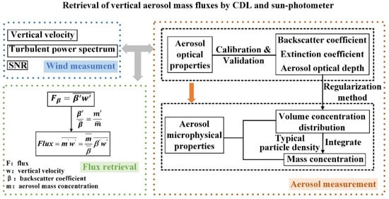
Figure 1.
Overview of aerosol mass fluxes retrieval procedure.
3. Experiment and Measurements
3.1. Experiment
To validate the aerosol optical properties retrieval method, three field experiments using a CDL and a sun photometer were conducted. The details of these experiments and CDL scanning mode setting were listed in Table 3 of Dai et al. (2021) [37]. Aerosol mass flux observations were carried out from 11 April to 20 April 2020 with a CDL and a sun photometer at the observation platform of Qingdao Leice Transient Technology Co., Ltd., which is located in the central area of Laoshan District and surrounded by many high buildings. From this dataset, a measurement case of a 24-h aerosol mass fluxes observation is selected and presented in Section 3.2.
3.2. A Measurement Case of a 24-h Vertical Aerosol Mass Fluxes Observation
In this work, the aerosol mass fluxes observation on 13 April 2020 was selected to be discussed. It was a clear day and the relative humidity on this day was less than 15% according to the measurement with the surface automatic weather station. In this day, the sunrise time was at 05:27 local standard time (LST) and the sunset time was at 18:30 LST. Figure 2 presents the diurnal variation of the SNR, the vertical velocity, and the aerosol backscatter coefficient at 1550 nm on 13 April 2020. To calculate the aerosol mass fluxes with EC method, the whole day was divided into 20 time periods which were separated with the black lines in Figure 2b,c. The time duration for fluxes calculation was chosen approximately as 72 min there, which is reasonable and in the range of 60 to 90 min that other study reported [9]. From Figure 2b, the updraft (in red and yellow colors) and downdraft (in blue color) can be clearly distinguished. The enhanced vertical mixing processes appeared during 09:00–18:00 LST and a strong updraft occurred during 13:30–15:00 LST. Additionally, the SNR of the CDL and aerosol backscatter coefficient at 1550 nm show similar tendencies. A downward process of aerosol occurred at about 1200 m height during the night as the red box framed in Figure 2a,c.
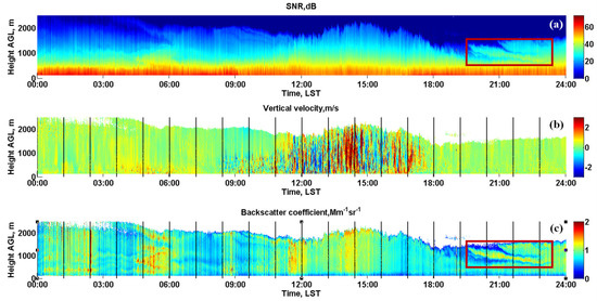
Figure 2.
The diurnal variation of (a) CDL system SNR, (b) vertical velocity and (c) aerosol backscatter coefficient at 1550 nm on 13 April 2020 (temporal resolution, 1 s; spatial resolution, 15 m).
Then, by inputting the aerosol optical properties at multi-wavelength and applying regularization inversion method, as mentioned above in Section 2.2.3, the aerosol volume concentration distribution could be retrieved. This method is validated with sun photometer measurements and two examples are presented in Figure 3. The aerosol size distributions could be distinguished with Ångström exponent from the sun photometer [35]. It could be indicated that coarse-mode particles (>1 μm) dominating when , while fine-mode particles (<1 μm) dominating when . When , it corresponds to coarse-mode particles and fine-mode particles which both exist, nevertheless with most of the particles in the fine-mode. During 14:06–15:29 LST on 15 March 2019, Figure 3a presents the retrieved aerosol volume concentration based on CDL data which shows the coarse-mode particles dominating and the same conclusion that could be drawn according to Figure 3b. During 10:45–12:22 LST on 24 September 2019, as shown in Figure 3c, most of the particles are in the fine-mode. In Figure 3d, the Ångström exponent is between 1 and 2 which reveals the same aerosol size distribution.

Figure 3.
Aerosol volume concentration distribution derived from CDL data and Ångström exponent from the sun photometer on 15 March 2019 (a,b) and 24 September 2019 (c,d), and data framed by blue box in (b,d) were corresponding results in time period that (a,c) showed (time period, labeled with blue font).
The profiles of the mean aerosol backscatter coefficients at 1550 nm and the mean aerosol mass concentrations are shown in Figure 4. The mean aerosol backscatter coefficients at 1550 nm and the mean aerosol mass concentrations show similar variation tendencies in Figure 4a–t. Before 10:48 LST, the aerosol backscatter coefficients and the mean aerosol mass concentrations clearly vary with height. However, after 10:48 LST, the aerosol backscatter coefficients and aerosol mass concentrations become constant with height until 18:00 LST. It may result from the radiation heating of near-surface and the enhanced vertical mixing process which leads to the well-mixed aerosol layer in the PBL. On the contrary, after 18:00 LST, because of the attenuated near-surface thermal radiation and the vertical mixing, the differences of aerosol backscatter coefficients and aerosol mass concentrations at different heights increase slowly again. From 19:12 LST to 22:48 LST, the downward process of aerosol is also found as the orange box framed in Figure 4q–s which is consistent with the phenomenon that Figure 2a,c shows. Then, the vertically averaged mean mass concentration between 120 m and about 2000 m, and the corresponding deviations of different time periods, are calculated and shown in Figure 5. The mean mass concentrations of different heights vary in the range of 15 to 30 with the minimum value of 15.4 and the maximum value of 27.4 . Before 06:00 LST, it stabilizes in the range of 20 to 27 . During 06:00–08:24 LST, it decreases to about 17 rapidly and then increases to the maximum value of 27.4 slowly until 14:24 LST. After 14:24 LST, it decreases and reaches the minimum value of 15.4 until 20:24 LST. Then, it increases to 22.1 at the end of the day.
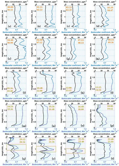
Figure 4.
Profiles of the mean aerosol backscatter coefficients at 1550 nm (blue dotted line) and the mean aerosol mass concentrations (black solid line) on 13 April 2020 (average time, about 72 min). The corresponding average time period is labeled with brown font and a downward process of aerosol is framed with the orange box in Figure 4q–s.
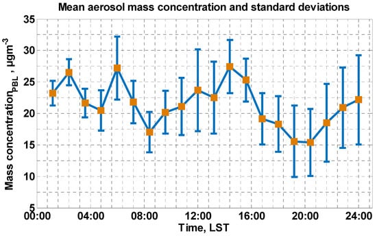
Figure 5.
The vertically averaged mean mass concentration between 120 m and about 2000 m (brown solid square) and the corresponding deviations (blue error bar) of different time periods on 13 April 2020.
Once the aerosol mass concentration is calculated, the aerosol mass fluxes can be estimated, as Section 2.2.3 introduced. Figure 6 shows the profiles of the vertical aerosol mass fluxes of all day. Before 07:12 LST, the vertical aerosol mass fluxes at all height levels are close to zero which means that the atmosphere is stable and that no obvious vertical transport processes existed. Then, the atmosphere is getting warmer with solar radiation, and upward vertical transports firstly appear near the surface and then gradually spread upward as orange box framed in Figure 6. After 12:00 LST, the values of the vertical aerosol mass fluxes in the whole PBL are all positive until 15:36 LST which means that upward vertical transports existed in the whole PBL in this time period. Then, the upward vertical transports get weaker with the decrease in radiation and attenuated convection activities. Therefore, the absolute values of the vertical aerosol mass fluxes are getting smaller and tend to zero once again. During 19:12–20:24 LST, there is an obvious downward transport (framed with a green box) at about 1200 m height which is consistent with the downward process of aerosol found in Figure 2c and Figure 4q,r.

Figure 6.
Profiles of the vertical aerosol mass fluxes on 13 April 2020 and the corresponding average time periods are labeled above each figure with black font.
The aerosol mass fluxes of each time period in the whole PBL are integrated and the results are shown in Figure 7. The values of the integrated vertical aerosol mass fluxes of the whole PBL are positive from 07:12 LST to 15:36 LST approximately, while close to zero during the other time periods. During 07:12–15:36 LST, the values of the integrated vertical aerosol mass fluxes increase and reach the maximum about 260 at 14:24 LST, and then decrease gradually. During this period, the integrated aerosol mass fluxes are positive which means the total vertical aerosol transport of the whole PBL is upward. Hence, it must be existed a divergence transport process of aerosols at the top of the PBL and a convergence transport process of aerosols near the ground. However, in this work, we focus on the aerosol vertical transport process rather than the horizontal transport process. In the further studies, both researches of aerosol vertical transport and horizontal transport will be achieved by combining other scanning models.
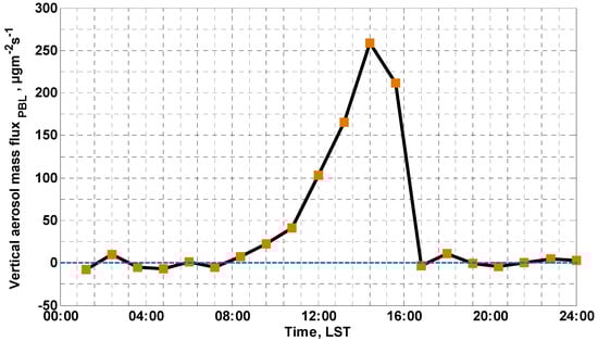
Figure 7.
Integrated aerosol mass fluxes of the whole PBL (brown solid square) on 13 April 2020.
Figure 8 shows the variance spectra on the time series of the vertical velocity and the aerosol backscatter coefficients at 1550 nm at three height levels during 12:00–13:12 LST. From Figure 8a, the variance spectra of the vertical velocity satisfy Kolmogorov’s −5/3 law when the frequency is smaller than 0.2 Hz. Thus, 0.2 Hz is set to be the frequency threshold for variance spectra of the vertical velocity and hence the instruments noise level can be estimated [33,45]. Similarly, 0.02 Hz is set to be the frequency threshold for variance spectra of the aerosol backscatter coefficient at 1550 nm, as Figure 8b shows. Then, the cospectrum of the vertical velocity and the aerosol backscatter coefficients of the same time period can be calculated, as shown in Figure 9. From this figure, it could be found that the turbulence, whose frequency ranges from 6 × 10⁻³ Hz to 9 × 10⁻⁴ Hz, makes significant contributions to the vertical aerosol mass fluxes.
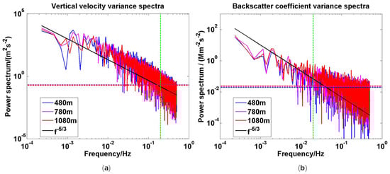
Figure 8.
Power spectral of the vertical velocity (a) and the aerosol backscatter coefficients at 1550 nm (b) for three heights including 480 m (blue solid line), 780 m (pink solid line) and 1080 m (red solid line) of 12:00–13:12 LST on 13 April 2020. Furthermore, an expected f −5/3 tendency (black solid line), threshold frequency (green dotted line), and noise level for different heights (dotted lines in blue, pink and red) are presented at the same time.
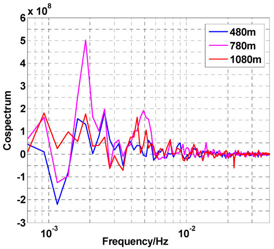
Figure 9.
Cospectrum of vertical velocity and aerosol backscatter coefficients at three heights, including 480 m (blue solid line), 780 m (pink solid line) and 1080 m (red solid line) of 12:00–13:12 LST on 13 April 2020.
3.3. Error Analysis
Finally, the relative errors of the vertical aerosol mass flux retrieval at three heights from 12:00 to 15:36 LST (three time periods) are summarized and listed in Table 1. The sample error is the main error in the flux retrieval [9,46] which cannot be avoided because of finite sample number and time duration. It could be estimated based on a previous study [18]. The instrument error is calculated as well [18], but it is much smaller than the sample error, thus it is not listed in Table 1. In this case, it is necessary to evaluate the relative error introduced from the aerosol optical properties retrieval with CDL data. The equation to estimate this is expressed as Equation (8):

Table 1.
Main errors of the vertical aerosol mass flux retrieval for three heights in 12:00–15:36 LST which including Sample error , aerosol optical properties retrieval error , and regularization retrieval error .
According to the previous study [27], the error from regularization method is no more than 50%.
4. Conclusions
In this paper, based on the aerosol optical properties retrieved by a calibrated CDL and the vertical wind velocities measured simultaneously, the EC method is applied to retrieve the vertical turbulent aerosol mass fluxes. A measurement case of 24-h fluxes observations is presented. The diurnal variation of vertical aerosol transport in the PBL and the main relative errors are discussed. The key conclusions are summarized as below:
- (1)
- By analyzing the variation processes of the vertical velocity, the aerosol backscatter coefficients at 1550 nm, and the vertical aerosol mass fluxes of 13 April 2020, it is found that, from 10:48 LST to 18:00 LST, the upward transport and the vertical mixture of aerosol are obvious in the PBL which may be caused by the radiation heating of near-surface and the enhanced vertical convection. During this time period, the aerosol backscatter coefficients tend to be constant with height in the PBL. Additionally, most of the aerosol mass fluxes values are positive which means that the upward transport process is in progress at the same period. In the other time periods, the vertical aerosol mass fluxes at all heights are nearly close to zero which means that the atmosphere is relatively stable and that there are few obvious vertical transport processes. The values of the integrated vertical aerosol mass fluxes of the whole PBL are positive from 07:12 LST to 15:36 LST approximately, while close to zero during the other time periods. During 07:12–15:36 LST, the values of the integrated vertical aerosol mass fluxes increase and reach the maximum of about 260 at 14:24 LST, and then decrease gradually.
- (2)
- A downward process of aerosol particles is observed at about 1200 m during 19:12–22:48 LST. Furthermore, during 19:12–20:24 LST, the aerosol mass flux values of the corresponding height are negative, which indicates that an ongoing downward transport process exists.
- (3)
- The vertically averaged mean mass concentration between 120 m and about 2000 m varies in the range of 15 to 30 , with the minimum value of 15.4 and the maximum value of 27.4 . It stabilizes before 06:00 LST and goes through two processes (firstly decreases and then increases).
- (4)
- Finally, the relative errors involved in the aerosol mass flux retrieval are evaluated. The sample error is the dominating error in flux retrieval and it increases with height, except during 12:00–13:12 LST. The instrument error which could be retrieved from the power spectra is much smaller than the sample error . Additionally, the aerosol optical properties retrieval error is 21% and error introduced from regularization method is less than 50%.
It should be emphasized that the results of the retrieved mass fluxes have not been validated with an independent measurement as for the absence of the independent validation instrument in this experiment. However, we could ensure that the values of fluxes are within expected ranges for the PBL through comparison with previous studies [9] and are also consistent with plausible diurnal patterns based on the boundary layer dynamics. In fact, our research focusing on validating the retrieval method and results with in-situ instruments equipped at one height on a meteorological tower is ongoing.
In the further study, there are plans to continue conducting combined observation of the CDL and the sun photometer, accumulate observation data, and try to explore the interaction between three-dimensional wind field and aerosol mixing development. Furthermore, the joint observations and the transport analyses of water vapor, carbon dioxide, and other trace gases would be considered and carried out by the combination of the CDL and other gas analyzers.
Author Contributions
All authors made great contributions to the presented work. Conceptualization, G.D., S.W. and X.W. (Xiaoye Wang); methodology, X.W. (Xiaoye Wang); software, X.W. (Xiaoye Wang); validation, K.S., G.D. and S.W.; supervision and project administration, S.W.; data curation, R.L., J.Y. and X.W. (Xitao Wang); writing—original draft preparation, X.W. (Xiaoye Wang); writing—review and editing, S.W., G.D., X.S. and W.C. All authors have read and agreed to the published version of the manuscript.
Funding
This work was supported by National Key Research and Development Program of China under grant 2019YFC1408002 and 2019YFC1408001 and the National Natural Science Foundation of China (NSFC) under grant 61975191 and 41905022. This work was also supported by Dragon 4 program which conducted by European Space Agency (ESA) and the National Remote Sensing Center of China (NRSCC) under grant 32296.
Data Availability Statement
Due to confidentiality agreements, supporting data can only be made available to bona fide researchers subject to a non-disclosure agreement. To get the data please contact to wush@ouc.edu.cn at Ocean University of China.
Acknowledgments
We thank our colleagues Qichao Wang and Xiangcheng Chen for their suggestions in original draft preparation, and also thank Dahai Wang from Qingdao Leice Transient Technology Co., Ltd. for preparing and operating the CDL.
Conflicts of Interest
The authors declare no conflict of interest.
References
- Boucher, O.; Randall, D.; Artaxo, P.; Bretherton, C.; Feingold, G.; Forster, P.; Kerminen, V.-M.; Kondo, Y.; Liao, H.; Lohmann, U.; et al. Clouds and aerosols. In Climate Change 2013: The Physical Science Basis. Contribution of Working Group I to the Fifth Assessment Report of the Intergovernmental Panel on Climate Change; Cambridge University Press: Cambridge, UK; New York, NY, USA, 2013; pp. 571–657. [Google Scholar]
- Buzorius, G.; Rannik, Ü.; Mäkelä, J.M.; Vesala, T.; Kulmala, M. Vertical aerosol particle fluxes measured by eddy covariance technique using condensational particle counter. J. Aerosol Sci. 1998, 29, 157–171. [Google Scholar] [CrossRef]
- Buzorius, G.; Rannik, Ü.; Nilsson, D.; Kulmala, M. Vertical fluxes and micrometeorology during aerosol particle formation events. Tellus B Chem. Phys. Meteorol. 2001, 53, 394–405. [Google Scholar] [CrossRef]
- Dorsey, J.; Nemitz, E.; Gallagher, M.; Fowler, D.; Williams, P.; Bower, K.; Beswick, K. Direct measurements and parameterisation of aerosol flux, concentration and emission velocity above a city. Atmos. Environ. 2002, 36, 791–800. [Google Scholar] [CrossRef]
- Mårtensson, E.; Nilsson, E.; Buzorius, G.; Johansson, C. Eddy covariance measurements and parameterisation of traffic related particle emissions in an urban environment. Atmos. Chem. Phys. 2006, 6, 769–785. [Google Scholar] [CrossRef]
- Nemitz, E.; Dorsey, J.; Flynn, M.; Gallagher, M.; Hensen, A.; Erisman, J.-W.; Owen, S.; Dämmgen, U.; Sutton, M. Aerosol fluxes and particle growth above managed grassland. Biogeosciences 2009, 6, 1627–1645. [Google Scholar] [CrossRef]
- Ruuskanen, T.M.; Kaasik, M.; Aalto, P.P.; Horrak, U.; Vana, M.; Mårtensson, M.; Yoon, Y.; Keronen, P.; Mordas, G.; Ceburnis, D.; et al. Concentrations and fluxes of aerosol particles during the LAPBIAT measurement campaign at Värriö field station. Atmos. Chem. Phys. 2007, 7, 3683–3700. [Google Scholar] [CrossRef]
- Baldocchi, D.; Falge, E.; Gu, L.; Olson, R.; Hollinger, D.; Running, S.; Anthoni, P.; Bernhofer, C.; Davis, K.; Evans, R.; et al. FLUXNET: A new tool to study the temporal and spatial variability of ecosystem-scale carbon dioxide, water vapor, and energy flux densities. Bull. Am. Meteorol. Soc. 2001, 82, 2415–2434. [Google Scholar] [CrossRef]
- Engelmann, R.; Wandinger, U.; Ansmann, A.; Müller, D.; Žeromskis, E.; Althausen, D.; Wehner, B. Lidar observations of the vertical aerosol flux in the planetary boundary layer. J. Atmos. Ocean. Technol. 2008, 25, 1296–1306. [Google Scholar] [CrossRef]
- Gal-Chen, T.; Xu, M.; Eberhard, W.L. Estimations of atmospheric boundary layer fluxes and other turbulence parameters from Doppler lidar data. J. Geophys. Res. 1992, 97, 18409–18423. [Google Scholar] [CrossRef]
- Mann, J.; Peña, A.; Bingöl, F.; Wagner, R.; Courtney, M. Lidar scanning of momentum flux in and above the atmospheric surface layer. J. Atmos. Ocean. Technol. 2010, 27, 959–976. [Google Scholar] [CrossRef]
- Smalikho, I.N.; Banakh, V.A. Measurements of wind turbulence parameters by a conically scanning coherent Doppler lidar in the atmospheric boundary layer. Atmos. Meas. Tech. 2017, 10, 4191–4208. [Google Scholar] [CrossRef]
- Penndorf, R. Tables of the refractive index for standard air and the Rayleigh scattering coefficient for the spectral region between 0.2 and 20.0 μ and their application to atmospheric optics. J. Opt. Soc. Am. 1957, 47, 176–182. [Google Scholar] [CrossRef]
- Eichinger, W.; Cooper, D.; Kao, J.; Chen, L.; Hipps, L.; Prueger, J. Estimation of spatially distributed latent heat flux over complex terrain from a Raman lidar. Agric. For. Meteorol. 2000, 105, 145–159. [Google Scholar] [CrossRef][Green Version]
- Behrendt, A.; Wulfmeyer, V.; Senff, C.; Muppa, S.K.; Späth, F.; Lange, D.; Kalthoff, N.; Wieser, A. Observation of sensible and latent heat flux profiles with lidar. Atmos. Meas. Tech. 2020, 13, 3221–3233. [Google Scholar] [CrossRef]
- Kiemle, C.; Ehret, G.; Fix, A.; Wirth, M.; Poberaj, G.; Brewer, W.; Hardesty, R.; Senff, C.; LeMone, M. Latent heat flux profiles from collocated airborne water vapor and wind lidars during IHOP_2002. J. Atmos. Ocean. Technol. 2007, 24, 627–639. [Google Scholar] [CrossRef]
- Fiorani, L.; Colao, F.; Palucci, A.; Poreh, D.; Aiuppa, A.; Giudice, G. First-time lidar measurement of water vapor flux in a volcanic plume. Opt. Commun. 2011, 284, 1295–1298. [Google Scholar] [CrossRef]
- Giez, A.; Ehret, G.; Schwiesow, R.L.; Davis, K.J.; Lenschow, D.H. Water vapor flux measurements from ground-based vertically pointed water vapor differential absorption and Doppler lidars. J. Atmos. Ocean. Technol. 1999, 16, 237–250. [Google Scholar] [CrossRef]
- Linné, H.; Hennemuth, B.; Bösenberg, J.; Ertel, K. Water vapour flux profiles in the convective boundary layer. Theor. Appl. Climatol. 2007, 87, 201–211. [Google Scholar] [CrossRef]
- Senff, C.; Bösenberg, J.; Peters, G. Measurement of water vapor flux profiles in the convective boundary layer with lidar and radar-RASS. J. Atmos. Ocean. Technol. 1994, 11, 85–93. [Google Scholar] [CrossRef]
- Wu, S.; Dai, G.; Song, X.; Liu, B.; Liu, L. Observations of water vapor mixing ratio profile and flux in the Tibetan Plateau based on the lidar technique. Atmos. Meas. Tech. 2016, 9, 1399–1413. [Google Scholar] [CrossRef]
- Gibert, F.; Koch, G.J.; Beyon, J.Y.; Hilton, T.W.; Davis, K.J.; Andrews, A.; Flamant, P.H.; Singh, U.N. Can CO2 turbulent flux be measured by lidar? A preliminary study. J. Atmos. Ocean. Technol. 2011, 28, 365–377. [Google Scholar] [CrossRef]
- Aiuppa, A.; Fiorani, L.; Santoro, S.; Parracino, S.; Nuvoli, M.; Chiodini, G.; Minopoli, C.; Tamburello, G. New ground-based lidar enables volcanic CO2 flux measurements. Sci. Rep. 2015, 5, 13614. [Google Scholar] [CrossRef]
- Fiorani, L.; Santoro, S.; Parracino, S.; Maio, G.; Nuvoli, M.; Aiuppa, A. Early detection of volcanic hazard by lidar measurement of carbon dioxide. Nat. Hazards 2016, 83, 21–29. [Google Scholar] [CrossRef]
- Senff, C.; Alvarez, R.; Mayor, S.; Zhao, Y. Ozone Flux Profiles in the Boundary Layer Observed with an Ozone DIAL/Doppler Lidar Combination. In Advances in Atmospheric Remote Sensing with Lidar; Springer: Berlin, Germany, 1997; pp. 363–366. [Google Scholar]
- Bennett, M.; Edner, H.; Grönlund, R.; Sjöholm, M.; Svanberg, S.; Ferrara, R. Joint application of Doppler Lidar and differential absorption lidar to estimate the atomic mercury flux from a chlor-alkali plant. Atmos. Environ. 2006, 40, 664–673. [Google Scholar] [CrossRef]
- Müller, D.; Wandinger, U.; Ansmann, A. Microphysical particle parameters from extinction and backscatter lidar data by inversion with regularization: Theory. Appl. Opt. 1999, 38, 2346–2357. [Google Scholar] [CrossRef]
- Chouza, F.; Reitebuch, O.; Benedetti, A.; Weinzierl, B. Saharan dust long-range transport across the Atlantic studied by an airborne Doppler wind lidar and the MACC model. Atmos. Chem. Phys. 2016, 16, 11581–11600. [Google Scholar] [CrossRef]
- Lv, L.; Liu, W.; Zhang, T.; Chen, Z.; Dong, Y.; Fan, G.; Xiang, Y.; Yao, Y.; Yang, N.; Chu, B.; et al. Observations of particle extinction, PM2.5 mass concentration profile and flux in north China based on mobile lidar technique. Atmos. Environ. 2017, 164, 360–369. [Google Scholar] [CrossRef]
- Lv, L.; Xiang, Y.; Zhang, T.; Chai, W.; Liu, W. Comprehensive study of regional haze in the North China Plain with synergistic measurement from multiple mobile vehicle-based lidars and a lidar network. Sci. Total Environ. 2020, 721, 137773. [Google Scholar] [CrossRef] [PubMed]
- Liu, C.; He, L.; Pi, D.; Zhao, J.; Lin, L.; He, P.; Wang, J.; Wu, J.; Chen, H.; Yan, P.; et al. Integrating LIDAR data and four-dimensional flux method to analyzing the transmission of PM2. 5 in Shenzhen. Phys. Chem. Earth 2019, 110, 81–88. [Google Scholar] [CrossRef]
- Wu, S.; Liu, B.; Liu, J.; Zhai, X.; Feng, C.; Wang, G.; Zhang, H.; Yin, J.; Wang, X.; Li, R.; et al. Wind turbine wake visualization and characteristics analysis by Doppler lidar. Opt. Express 2016, 24, A762–A780. [Google Scholar] [CrossRef] [PubMed]
- Zhai, X.; Wu, S.; Liu, B.; Song, X.; Yin, J. Shipborne Wind Measurement and Motion-Induced Error Correction of a Coherent Doppler Lidar over the Yellow Sea in 2014. Atmos. Meas. Tech. 2018, 11, 1313–1331. [Google Scholar] [CrossRef]
- Zhai, X.; Wu, S.; Liu, B. Doppler lidar investigation of wind turbine wake characteristics and atmospheric turbulence under different surface roughness. Opt. Express 2017, 25, A515–A529. [Google Scholar] [CrossRef] [PubMed]
- Schuster, G.L.; Dubovik, O.; Holben, B.N. Angstrom exponent and bimodal aerosol size distributions. J. Geophys. Res. Atmos. 2006, 111, D07207. [Google Scholar] [CrossRef]
- Müller, D.; Ansmann, A.; Mattis, I.; Tesche, M.; Wandinger, U.; Althausen, D.; Pisani, G. Aerosol-type-dependent lidar ratios observed with Raman lidar. J. Geophys. Res. Atmos. 2007, 112, D16202. [Google Scholar] [CrossRef]
- Dai, G.; Wang, X.; Sun, K.; Wu, S.-H.; Song, X.; Li, R.; Yin, J.; Wang, X. Calibration and retrieval of aerosol optical properties measured with Coherent Doppler Lidar. J. Atmos. Ocean. Technol. 2021, 38, 1035–1045. [Google Scholar]
- Van Dingenen, R.; Raes, F.; Putaud, J.-P.; Baltensperger, U.; Charron, A.; Facchini, M.-C.; Decesari, S.; Fuzzi, S.; Gehrig, R.; Hansson, H.-C. A European aerosol phenomenology—1: Physical characteristics of particulate matter at kerbside, urban, rural and background sites in Europe. Atmos. Environ. 2004, 38, 2561–2577. [Google Scholar] [CrossRef]
- Ma, X.; Huang, Z.; Qi, S.; Huang, J.; Zhang, S.; Dong, Q.; Wang, X. Ten-year global particulate mass concentration derived from space-borne CALIPSO lidar observations. Sci. Total Environ. 2020, 721, 137699. [Google Scholar] [CrossRef]
- Papayannis, A.; Nicolae, D.; Kokkalis, P.; Binietoglou, I.; Talianu, C.; Belegante, L.; Tsaknakis, G.; Cazacu, M.; Vetres, I.; Ilic, L. Optical, size and mass properties of mixed type aerosols in Greece and Romania as observed by synergy of lidar and sunphotometers in combination with model simulations: A case study. Sci. Total Environ. 2014, 500, 277–294. [Google Scholar] [CrossRef]
- Haarig, M.; Walser, A.; Ansmann, A.; Dollner, M.; Althausen, D.; Sauer, D.; Farrell, D.; Weinzierl, B. Profiles of cloud condensation nuclei, dust mass concentration, and ice-nucleating-particle-relevant aerosol properties in the Saharan Air Layer over Barbados from polarization lidar and airborne in situ measurements. Atmos. Chem. Phys. 2019, 19, 13773–13788. [Google Scholar] [CrossRef]
- Gasteiger, J.; Groß, S.; Freudenthaler, V.; Wiegner, M. Volcanic ash from Iceland over Munich: Mass concentration retrieved from ground-based remote sensing measurements. Atmos. Chem. Phys. 2011, 11, 2209–2223. [Google Scholar] [CrossRef]
- Wang, T.; Han, Y.; Hua, W.; Tang, J.; Huang, J.; Zhou, T.; Huang, Z.; Bi, J.; Xie, H. Profiling Dust Mass Concentration in Northwest China Using a Joint Lidar and Sun-Photometer Setting. Remote Sens. 2021, 13, 1099. [Google Scholar] [CrossRef]
- Zhang, R.; Duhl, T.; Salam, M.T.; House, J.M.; Flagan, R.C.; Avol, E.L.; Gilliland, F.D.; Guenther, A.; Chung, S.H.; Lamb, B.K. Development of a regional-scale pollen emission and transport modeling framework for investigating the impact of climate change on allergic airway disease. Biogeosciences 2013, 10, 3977. [Google Scholar] [PubMed]
- Chouza, F.; Reitebuch, O.; Jähn, M.; Rahm, S.; Weinzierl, B. Vertical wind retrieved by airborne lidar and analysis of island induced gravity waves in combination with numerical models and in situ particle measurements. Atmos. Chem. Phys. 2016, 16, 4675–4692. [Google Scholar] [CrossRef]
- Lenschow, D.; Mann, J.; Kristensen, L. How long is long enough when measuring fluxes and other turbulence statistics? J. Atmos. Ocean. Technol. 1994, 11, 661–673. [Google Scholar] [CrossRef]


Publisher’s Note: MDPI stays neutral with regard to jurisdictional claims in published maps and institutional affiliations. |
© 2021 by the authors. Licensee MDPI, Basel, Switzerland. This article is an open access article distributed under the terms and conditions of the Creative Commons Attribution (CC BY) license (https://creativecommons.org/licenses/by/4.0/).