Article

Synergistic Calibration of a Hydrological Model Using Discharge and Remotely Sensed Soil Moisture in the Paraná River Basin

by
Ayan Santos Fleischmann
1,*,
Ahmad Al Bitar
2,
Aline Meyer Oliveira
1,3,
Vinícius Alencar Siqueira
1,
Bibiana Rodrigues Colossi
1,
Rodrigo Cauduro Dias de Paiva
1,
Yann Kerr
2,
Anderson Ruhoff
1,
Fernando Mainardi Fan
1,
Paulo Rógenes Monteiro Pontes
4 and
Walter Collischonn
1
1
Instituto de Pesquisas Hidráulicas (IPH), Universidade Federal do Rio Grande do Sul (UFRGS), Porto Alegre 91501-970, Brazil
2
Centre d’Etudes Spatiales de la Biosphère (CESBIO), Toulouse University (CNES, CNRS, INRAe, IRD, UPS), 31013 Toulouse, France
3
Department of Geography, University of Zurich, 8057 Zurich, Switzerland
4
Instituto Tecnológico Vale–Desenvolvimento Sustentável (ITV-DS), Belém 66055-090, Brazil
*
Author to whom correspondence should be addressed.
Remote Sens. 2021, 13(16), 3256; https://doi.org/10.3390/rs13163256
Submission received: 27 May 2021 / Revised: 6 August 2021 / Accepted: 11 August 2021 / Published: 18 August 2021

Abstract

:
Hydrological models are useful tools for water resources studies, yet their calibration is still a challenge, especially if aiming at improved estimates of multiple components of the water cycle. This has led the hydrologic community to look for ways to constrain models with multiple variables. Remote sensing estimates of soil moisture are very promising in this sense, especially in large areas for which field observations may be unevenly distributed. However, the use of such data to calibrate hydrological models in a synergistic way is still not well understood, especially in tropical humid areas such as those found in South America. Here, we perform multiple scenarios of multiobjective model optimization with in situ discharge and the SMOS L4 root zone soil moisture product for the Upper Paraná River Basin in South America (drainage area > 900,000 km²), for which discharge data for 136 river gauges are used. An additional scenario is used to compare the relative impacts of using all river gauges and a small subset containing nine gauges only. Across the basin, the joint calibration (CAL-DS) using discharge and soil moisture leads to improved precision and accuracy for both variables. The discharges estimated by CAL-DS (median KGE improvement for discharge was 0.14) are as accurate as those obtained with the calibration with discharge only (median equal to 0.14), while the CAL-DS soil moisture retrieval is practically as accurate (median KGE improvement for soil moisture was 0.11) as that estimated using the calibration with soil moisture only (median equal to 0.13). Nonetheless, the individual calibration with discharge rates is not able to retrieve satisfactory soil moisture estimates, and vice versa. These results show the complementarity between these two variables in the model calibration and highlight the benefits of considering multiple variables in the calibration framework. It is also shown that, by considering only nine gauges instead of 136 in the model optimization, the model is able to estimate reasonable discharge and soil moisture, although relatively less accurately and with less precision than for the entire dataset. In summary, this study shows that, for poorly gauged tropical basins, the joint calibration of SMOS soil moisture and a few in situ discharge gauges is capable of providing reasonable discharge and soil moisture estimates basin-wide and is more preferable than performing only a discharge-oriented optimization process.

Graphical Abstract

1. Introduction

Hydrological models are powerful tools for water resources management and comprehension of the water cycle, yet the estimation of realistic model parameters and prediction in ungauged basins (PUB) [1] are still great challenges for hydrologists, even though major advances have been made in understanding such processes [2]. While the typical calibration process for hydrological models mainly involves the use of discharge data, recent efforts by the hydrological community have aimed at simultaneously correcting the representation of the water cycle components (e.g., soil moisture and evapotranspiration dynamics) instead of focusing only on discharge estimation. This leads to parsimonious models that are capable of providing the right estimates for the right reasons [3,4].
While hydrological data scarcity has always been an issue for hydrological modeling [1], the era of open-access earth observation (EO) data [5] has brought about a wealth of observations to address this topic [6,7], especially for large basins. Remote sensing soil moisture observations can be retrieved using microwave techniques, such as synthetic aperture radar (SAR) (e.g., ERS-1, ERS-2) or passive radiometer (e.g., AMSR-E) techniques. Combinations of multiple active and passive sensors are also possible (e.g., ESA-CCI). More recently, the first missions dedicated to estimating global soil moisture from L-Band observations were launched: the Soil Moisture Ocean Salinity Mission (SMOS) [8], launched in 2009, which provides soil moisture information every three days with a spatial resolution of 40 km; and the Soil Moisture Active and Passive (SMAP) [9] mission, launched in 2015. These advances have contributed to the development of global multidecadal datasets of soil moisture [10], fostering the hydrological monitoring of agricultural lands [11] and extreme events such as droughts and floods [12,13], as well as offering the potential to better inform and constrain hydrological models [14], particularly for explicitly accounting soil moisture models, where the soil water balance is the core of the model structure.
The integration of remotely sensed (RS) soil moisture data with hydrological models has been addressed through validation [15], calibration [16,17,18,19,20,21,22], and data assimilation [19,23,24,25,26,27,28,29,30] frameworks. Model calibration and data assimilation experiments have not been conclusive and have suggested both moderate improvements [16,22,29,31] and also no impact in terms of model performance [20,21]. On one hand, Campo et al. [17] and Nijzink et al. [32] observed improvements in streamflow prediction when coupling remotely sensed soil moisture to discharge data in a calibration scheme. Parajka et al. [16] and Tong et al. [22] found that the coupled approach resulted in more robust model parameters, while Milzow et al. [18] highlighted the importance of soil moisture data to identify errors in precipitation inputs.
Conversely, López et al. [20] found that even though the coupled approach resulted in reasonable estimates of streamflow, better model performance was achieved when remote sensing observations were not included in the calibration scheme. Li et al. (2018) reported degradation of the streamflow performance with the joint approach at some locations, while Koppa et al. [21] reported that the coupled calibration strategy might not always be valuable because of the trade-offs in accuracy among model responses. These trade-offs were also discussed by Dembélé et al. [33], in which the model performance in terms of discharge was decreased, but a simultaneous increase in performance for soil moisture indicated the benefits of using multiple spatially distributed observations for model calibration. The conclusions related to the added value of soil moisture for hydrological modeling depend on factors such as the model structure, applied techniques, how the model performance is evaluated, the observation operator (rescaling and filtering), and the scale mismatch between observations and models [6,34].
Major gaps remain in the context of model calibration with RS data. To our knowledge, no previous study has properly investigated the use of remotely sensed soil moisture for hydrological model calibration in South America. Meyer Oliveira et al. [35] reported the benefits of using soil moisture observations for an Amazonian sub-basin (Purus River Basin), but did not explore the spatial information for remotely sensed observations to its potential, so major questions remain as to whether model calibration is feasible in such humid areas and to what extent can remotely sensed soil moisture observations contribute to improve model realism. Studies on the calibration of models for very large domains (>100,000 km²) are also scarce (e.g., Koppa et al. [21] in the Mississippi basin (3.3 million km²), Sutanudjaja et al. [23] in the Rhine-Meuse basin (200,000 km²), Milzow et al. [18] in the Okavango river (170,000 km²), and Xu et al. [36] in the Great Lakes basin (1 million km²)), as the application of such techniques faces challenges regarding landscape heterogeneity and the need to correctly represent river water transport processes. Here, we present a case study in the Upper Paraná River Basin (~910,000 km²), a major tropical basin that poses several challenges for soil moisture representation at large scales, including its heterogeneous lithology and the presence of multiple dams, urban areas, and irrigation schemes that have the potential to hinder RS soil moisture retrieval. We also investigate for the first time the use of the SMOS L4 root zone soil moisture product [37] to calibrate a hydrological model. Our goal is to investigate the complementarity between in situ discharge and RS soil moisture for estimating large-scale distributed model parameters, improving the accuracy of the predictions of both variables, reducing parameter equifinality, and improving the water cycle representation in general. The model calibration is assessed in a distributed way in order to assess the impacts of the basin heterogeneity into the algorithm performance.

2. Materials and Methods

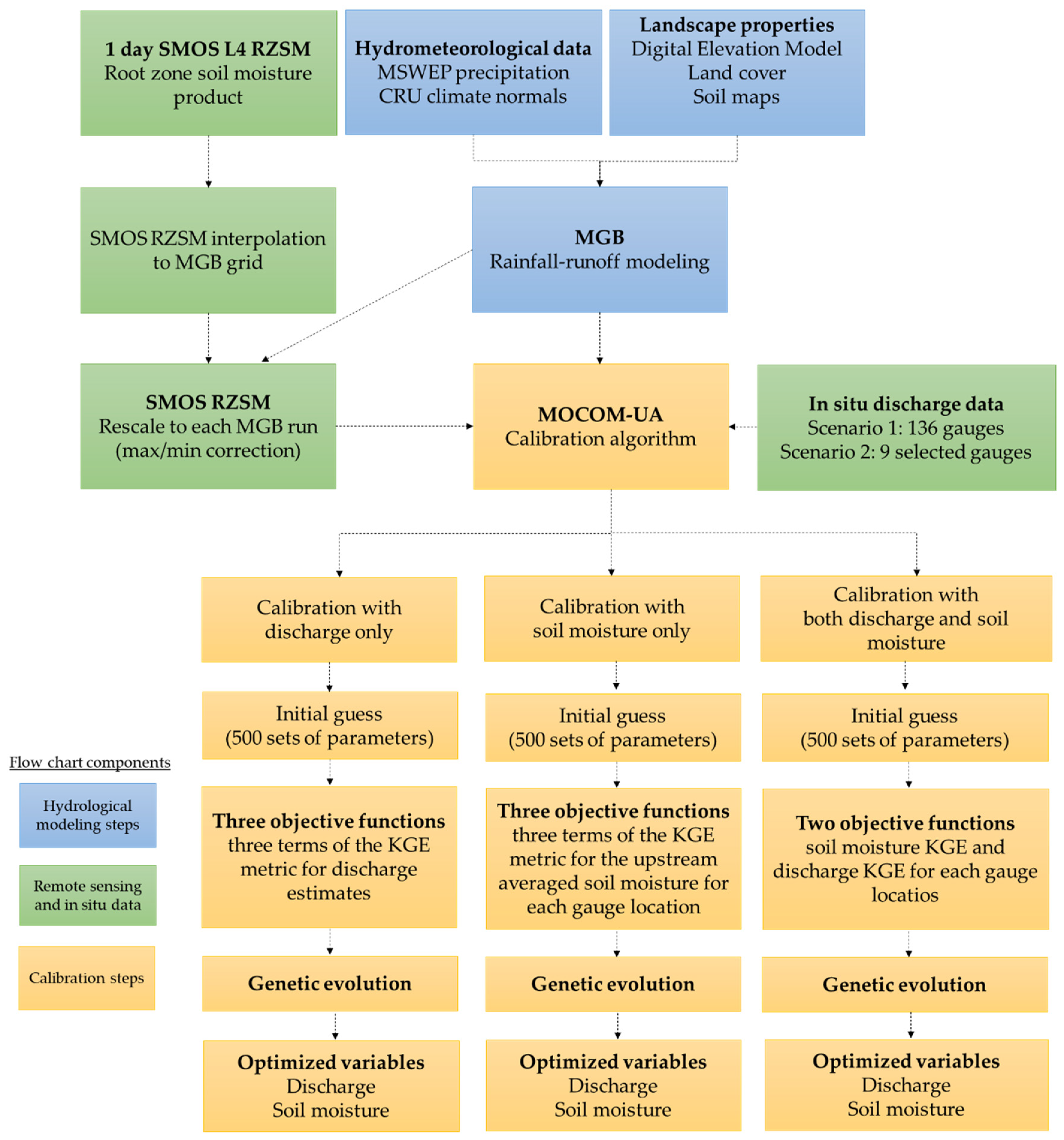
2.1. Research Overview

The MGB hydrological model [38] was applied to the Paraná River Basin and calibrated with in situ discharge and SMOS L4 root zone soil moisture data. Because of its large extents and peculiar characteristics, the Paraná River Basin covers a wide range of climatic, topographic, and pedological characteristics, which result in a variety of hydrological responses. The MOCOM-UA automatic calibration procedure [39] is used here to evaluate the impacts of using both soil moisture and discharge data to improve the hydrological model estimates. Figure 1 summarizes the adopted methodology, which is detailed in the following sections.

2.2. SMOS L4 Root Zone Soil Moisture Product

The L4 Root Zone Soil Moisture (L4 RZSM) [40] data used in this study were derived from the SMOS L3SM soil moisture product [41]. The SMOS mission [8] is part of the European Space Agency (ESA) earth explorer mission, with contribution from the French Space Agency (CNES) and the Spanish Centre for the Development of Industrial Technology (CDTI). It was specifically designed for the monitoring of surface soil moisture at the global scale, with a 3-day revisit at the equator at a nominal resolution of 40 km. The SMOS instrument is a 2D interferometric radiometer operating at 1.4 GHz (L-band) and providing multiangular full-polarization acquisitions. The SMOS L3SM product contains soil moisture maps over the EASE 25 km grid for ascending and descending orbits with a vertical sampling rate of 0–5 cm [42]. The L4 RZSM product provides volumetric root zone soil moisture (m3/m3) by applying a modified implementation of the Stroud exponential model [43] to the L3SM by considering a hydraulic-conductivity-based lag function. The product is provided with a quality flag that depends on error prone features such as the radio frequency interference (RFI), fraction of forested areas, and surface temperature. The L3SM is filtered for RFI in the pre-processing stage (RFI_Prob < 0.3). The hydraulic conductivity is computed based on the soil texture. The root zone soil moisture is obtained from the layer thickness weighted average of two layers (0–30 cm and 30 cm–1 m). It is available as operational daily and open data from the Centre Aval de Traitement des Données SMOS (CATDS) production center at Ifremer (L’Institut Français de Recherche pour l’Exploitation de la Mer), starting January 2020 (available at ftp://ext-catds-cpdc:[email protected]/Land_products/GRIDDED/L4SM, accessed on 17 August 2021). Data from 2010 to 2020 are also available from CATDS at ftp://ext-catds-cecsm:[email protected]/Land_products/L4_Root_Zone_Soil_Moisture/ (accessed on 17 August 2021). Daily data were downloaded in NetCDF format from the link above and processed in MATLAB (reading and extraction of points of interest inside our study area).

2.3. In Situ Discharge Data

A total of 136 in situ gauges from ANA (Brazilian National Water Agency; http://www.snirh.gov.br/hidroweb/; accessed on 17 August 2021) and ONS (Brazilian Electric System National Operator; http://www.ons.org.br/; accessed on 17 August 2021) were used. Since discharges in the basin are largely regulated by several reservoirs, naturalized streamflow series were used in the model calibration and verification, which were obtained from ONS. The gauges were split into two groups for the calibration scenarios: (i) a set of nine gauges associated with the most downstream gauges for each of the major Paraná tributaries plus the naturalized flow data for the Itaipu dam location in the downstream Paraná river (G9); (ii) a set containing all 136 available gauges (G136). The G9 set ensures an even distribution of gauges basin-wide, instead of G136, which is unevenly distributed, with a higher density in the left riverbank tributaries due to political borders.

2.4. MGB Model

MGB is a semi-distributed hydrological model [44] that has been widely used for large-scale simulations in South America [38,44,45] (model available at https://www.ufrgs.br/lsh/; accessed on 17 August 2021). The model was chosen for this study given its previous satisfactory applications in South America and its recent use for automatic calibration with remote sensing data [35]. Within the model, the basin is divided into unit catchments, while each one is divided into hydrologic response units (HRUs). The runoff generated in each HRU is routed through three linear reservoirs within the unit catchment (i.e., hillslope routing; the reservoirs are divided into surface, subsurface, and groundwater reservoirs) and then along the stream network with either Muskingum–Cunge or hydrodynamic methods [46,47]. The runoff generation mechanism is based on the ARNO saturation excess model [48], while the soil reservoir is conceptualized as a bucket with only one soil layer. The energy budget and evapotranspiration from the soil, vegetation, and wet canopy to the atmosphere are estimated using the Penman–Monteith equation, following the approach by Wigmosta et al. [49]. Soil moisture simulated by the MGB model is evaluated here in terms of the soil saturation degree. For a given unit catchment and time step, the soil saturation degree is computed as the ratio between the average available water in the soil and the average maximum storage capacity, both weighted by the HRU fraction within the unit catchment. For a given unit catchment and HRU, Equation (1) shows how the soil water balance is computed:
W i , j t = W i , j t 1 + ( P i , j E T i , j D s u p i , j D i n t i , j D b a s i , j + D c a p i , j )
where W i , j t is the water stored in the soil layer at the end of the time step at unit catchment i, in HRU j; W i , j t 1   is the water stored in the soil layer at the beginning of the time step; P i , j is the precipitation reaching the soil; E T i , j is the evapotranspiration; D s u p i , j is the surface runoff; D i n t i , j the subsurface flow; and D b a s i , j and D c a p i , j are the flow to the aquifer and from the aquifer to the soil layer, respectively. All variables are in mm.

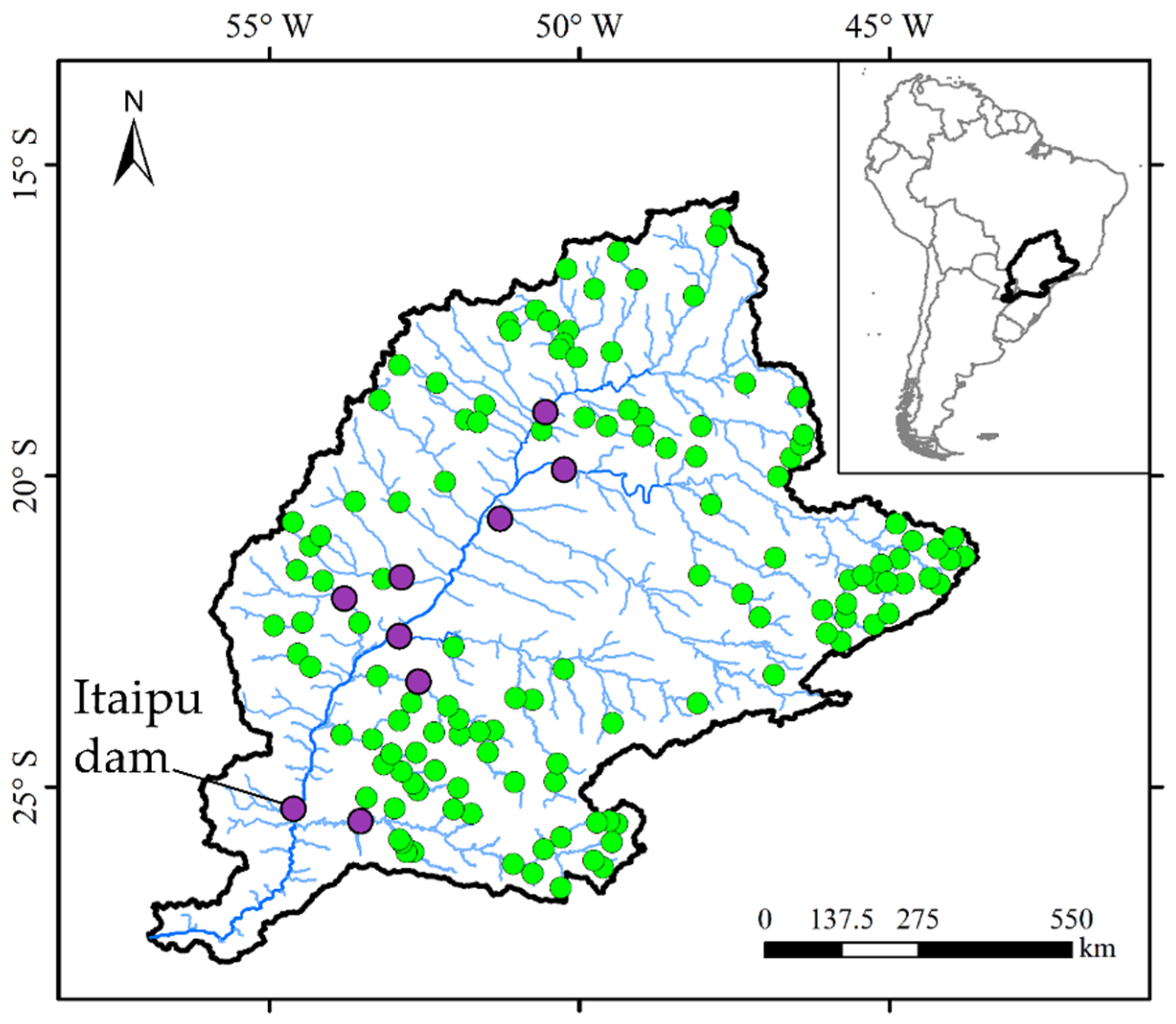
2.5. Model Application to the Upper Paraná River Basin

The Paraná is one of the longest rivers in the world (second in South America) and the main tributary of the La Plata Basin in South America (the fifth largest basin in the world) [50,51] (Figure 2). This study focuses on the Upper Paraná Basin (drainage area ~910,000 km2), which includes the most industrialized and urbanized region in Brazil. The basin supplies water for intensively irrigated agriculture, industry, and human supply and plays an important role in the Brazilian hydropower system, including the large Itaipu dam. Climate variability in the Upper Paraná Basin is pronounced due to its large spatial extent—the northern region has a warm, strongly seasonal precipitation regime, while the southern part features a more temperate climate and more evenly distributed precipitation over the year. From a hydrogeological perspective, the basin is also very heterogeneous, ranging from highly permeable sandstone rocks in the western regions to an impermeable igneous geology in the north, east, and part of the south. The basin was selected due to its heterogeneity in multiple aspects, which poses major challenges for soil moisture representations at large scales in hydrological models.
Regarding the model setup, the basin was divided into 1424 unit catchments measuring 641 km2 in area on average each (standard deviation of 573 km2). The model was forced with daily precipitation from MSWEP 2.1 [52], which was interpolated to the unit catchment centroid with the inverse distance weighting (IDW) method. A major distinction in terms of data availability occurs from the left (highly dense) to the right margins of the Paraná Basin, in accordance with the Brazilian political borders. In situ estimates of climate normals (1960–1990 long-term averages) for surface air temperature, wind speed, atmospheric pressure, relative humidity, and solar radiation were obtained from 195 stations from the Brazilian National Institute of Meteorology (INMET). These data were used to estimate evapotranspiration with the Penman–Monteith equation. The SRTM digital elevation model [53] was used to extract stream networks and delineate unit catchments with 90 m spatial resolution. The HRU map was derived from the South American product used by Fan et al. [54] at 400 m resolution (available at www.ufrgs.br/lsh/products; accessed on 17 August 2021), based on the combination of soil (classified into shallow and deep soils) and land use maps (classified into forest, agriculture, grasslands, wetlands, and urban areas). The Muskingum–Cunge routing method was adopted (instead of the hydrodynamic method) because of its much lower computational burden, which enables automatic calibration for large basins such as the Paraná. Table 1 summarizes the used input data.

2.6. Calibration Experiments and Assessed Metrics

The MOCOM-UA optimization algorithm (multiple-objective complex evolution–University of Arizona [39]) was adopted for automatic calibration in the MGB model. In a nutshell, the algorithm evolves a set of different initial parameters (i.e., initial guess individuals) towards the Pareto front. It treats the global search as a process of natural evolution, where each individual of the initial guess is a potential “parent” with a probability of participating in a process of reproduction. It uses rank-based selection to produce new points (i.e., the offspring) that are on average better than the original ones (parents) by using concepts of the SCE-UA (shuffled complex evolution [56]) scheme. The evolution stops when none of the individuals outperforms the others considering all of the evaluated objective functions. Here, a total of 500 individuals were adopted.
Three calibration scenarios were carried out according to the following objective functions: (i) minimize the discharge errors (i.e., calibration with discharge only; hereafter CAL-D); (ii) minimize the simulated soil moisture errors (i.e., calibration with soil moisture only; hereafter CAL-S); (iii) minimize both discharge and soil moisture errors (i.e., calibration with both variables; hereafter CAL-DS). The errors were evaluated using the Kling–Gupta efficiency metric (KGE [57]). For the calibration scenario (iii), two objective functions were used: the KGE between SMOS RZSM and MGB soil moisture; and the KGE between the simulated and observed river discharge. As MOCOM-UA is a multiobjective procedure, for calibrations (i) and (ii) the KGE metrics were split into three cost functions ( O F 1 , O F 2 , and O F 3 ):
O F 1 = ( σ s i m σ o b s 1 ) 2
O F 2 = ( r 1 ) 2
O F 3 = ( u s i m u o b s 1 ) 2
where σ s i m and σ o b s are the standard deviation values for the simulated and observed variables, respectively; r is the Pearson linear correlation; u s i m and u o b s are the long term averages for the simulated and observed variables, respectively.
To ensure comparability between soil moisture and discharge estimates and to make the best use of the spatially distributed nature of the remote sensing data, the calibration was performed in a gauge-oriented way, i.e., soil moisture values were averaged for the upstream area of each assessed gauge. For each gauge, the SMOS pixel centroids that fell within the upstream drainage area were considered for computing the soil moisture average. Furthermore, SMOS RZSM data were rescaled to MGB maximum and minimum soil saturation degree values. In addition, the three calibration scenarios were performed twice, firstly for the set of 136 discharge gauges (G136) and then for the set with nine selected gauges (G9). The set with nine gauges is only used in Section 3.4, which compares the performances for the two cases of gauge availability. Seven model parameters were calibrated (Table 2), which were set as uniform for the whole basin. The a priori parameter distribution followed a uniform distribution, with parameter sampling within a range of 10% to 400% of the average parameter values obtained from the MGB South American application [45]. The calibration was run for the period 1 January 2010–31 October 2017, which was chosen based on the precipitation, discharge, and SMOS data availability.
The results were evaluated in terms of soil moisture and discharge KGE values for each gauge. Figure 3 provides an example for a hypothetical gauge for a given calibration scenario, with 500 individuals used for the initial sets and 500 used for the optimized sets. To summarize all individuals, three metrics were computed: (i) improvement in discharge accuracy (∆KGED in Figure 3), which quantifies the overall performance of the solution; (ii) improvement in soil moisture accuracy (∆KGES), which represents the dispersion around the solution; (iii) overall precision gain ( Dist ini ¯   /   Dist end ¯ ), which accounts for the combined increase in both discharge and soil moisture performance precision with the optimization procedure. We stress that this metric is based on the increase of performance precision. The improvements in discharge and soil moisture accuracy are evaluated by the difference between the average of the optimized KGE values and the average of initial KGE values.
The overall precision gain is assessed firstly by computing the average distance between all individual initial KGE values and the median value (Distini in Figure 3), then by dividing it by the average distance obtained for the optimized KGE values (Distend in Figure 3). This is summarized in the scheme in Figure 3. The improvement in discharge accuracy (∆KGED) is computed as (KGED,end − KGED,ini), where KGED,end is the average discharge KGE for all optimized individuals and KGED,ini is the average KGE for the initial sets. The same is computed for the soil moisture accuracy (∆KGES = KGES,end − KGES,ini).
Finally, to understand the effects of landscape and climate heterogeneity on the optimization results, three aspects were considered: lithology types, irrigation areas from ANA [58], and precipitation seasonality computed with the method by Walsh and Lawler [59].

3. Results

3.1. Calibration Results and Model Performance Improvement

Overall, both discharge and soil moisture predictions were improved basin-wide in all calibration scenarios when compared to the initial random estimation (Figure 4). Since soil moisture data were aggregated at the sub-basin scale, in order to ensure the comparability between the calibrations with discharge gauges and distributed soil moisture data (see Section 2.6), the model performance for soil moisture is also presented at the gauge locations. As expected, the CAL-D scenario led to more accurate discharge and the CAL-S to more accurate soil moisture estimates. The CAL-DS scenario, which considered both discharge and soil moisture in the objective function, was able to improve both variables, leading to discharge estimates as accurate as those obtained with CAL-D, with the same for soil moisture in the CAL-S scenario. CAL-DS led to performance degradation for a limited number of gauges. The median improvements in discharge accuracy were 0.14, −0.02 and 0.14 for CAL-D, CAL-S, and CAL-DS, respectively; while the median values for soil moisture accuracy were 0.05, 0.13 and 0.11, for CAL-D, CAL-S, and CAL-DS, respectively.
When analyzing individual gauges, a relatively well-defined Pareto region was identified for the CAL-DS estimates (Figure 5). This led to higher precision (i.e., smaller dispersion) among optimized parameter sets for both soil moisture and discharge, as evidenced by the higher median overall precision gain obtained with the CAL-DS scenario; the median values were 4.42, 3.10, and 9.20 for CAL-D, CAL-S, and CAL-DS, respectively. This also led to improvements in both soil moisture and discharge accuracy. CAL-S not only led to less accurate discharge estimates but also to more disperse ones, while the opposite occurred for CAL-D. It is interesting to note that CAL-D led to more dispersed discharges (in terms of model performance) than did CAL-S for soil moisture, for which all of the optimized solutions converged to very similar soil moisture KGE values (e.g., KGES,end around 0.92 for gauge 9 in Figure 5 for the CAL-S scenario). This may have been related to the different sensitivity levels of the soil moisture and discharge to the KGE metric. The most downstream gauge, close to Itaipu dam (gauge 7 in Figure 5; 827,000 km2), clearly showed that the calibration with discharge largely improved the discharge results, although much less so for soil moisture and vice versa, while CAL-DS improved both. Supplementary Figure S1 shows discharge and soil moisture time series for Itaipu, depicting the relatively smaller dispersion in the CAL-DS scenario in comparison to CAL-D and CAL-S. The poor discharge representation by the CAL-S scenario for Itaipu (gauge 7 in Figure 5) occurred because of underestimated values during the low flow periods (Figure S1).
At the entire basin scale, there was an overall precision gain, estimated as ( Dist ini ¯   /   Dist end ¯ ), for all gauges, which is a natural outcome of the optimization procedure; however, while the gain was higher than 8 for most gauges in the CAL-DS scenario (Figure 4), this was also associated with degradation in the discharge accuracy for a few gauges, i.e., for these specific locations the optimization led to more precise yet less accurate estimates.

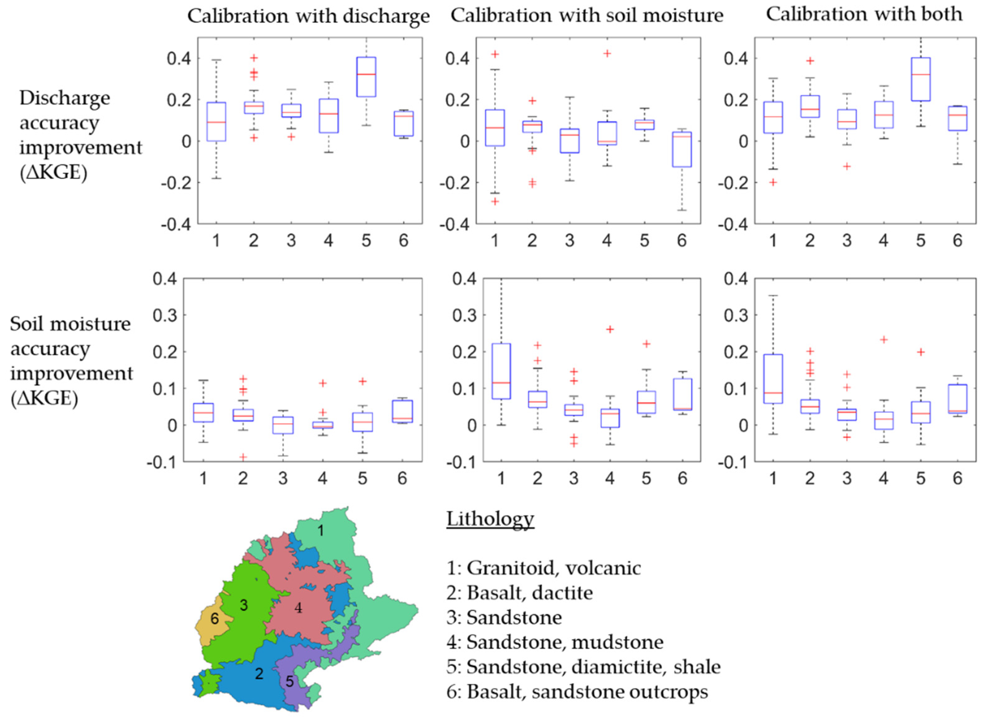
3.2. Impacts of Geology, Anthropogenic Activities, and Precipitation Seasonality on Model Optimization

Many factors can explain the model responses to different calibration setups. The different calibration setups in the Paraná Basin were analyzed with respect to homogeneous regions of geological (lithology) and anthropogenic activities (irrigation areas), as well as precipitation (seasonality) characteristics (Figure 6 and Figure 7). The results showed that the most relevant feature that affected the optimization outputs was lithology, which was tightly related to soil and groundwater storage dynamics.
Regarding lithology types, six main regions were defined in the basin (Figure 6). The CAL-DS scenario led to very similar behavior to the CAL-D when assessing discharge accuracy improvements (i.e., greatest improvement for lithology type 5) and to the CAL-S scenario when assessing soil moisture improvements (i.e., greatest improvement for lithology type 1).
When calibrating with both discharge and soil moisture (CAL-DS) parameters, the greatest precision improvements were mostly obtained for sandstone areas (regions 3, 5, and 6; Figure 7a) and regions with high irrigation rates (Figure 7b). The calibration with discharge data led to similar behavior for the lithology types, although no distinction occurred regarding irrigation areas and precipitation seasonality. In turn, the calibration with soil moisture led to a different result, with the highest precision improvement occurring in the upstream granitoid and volcanic areas (region 1), as well as in regions with the highest seasonal precipitation (Figure 7c). No clear relationships were obtained when relating overall precision gain and accuracy improvements for discharge and soil moisture with the upstream drainage area, irrigation areas, and precipitation seasonality for the set of 136 gauges (Figure S2), except that for small drainage and irrigation areas the performance was very noisy, which was not observed for the precipitation seasonality.

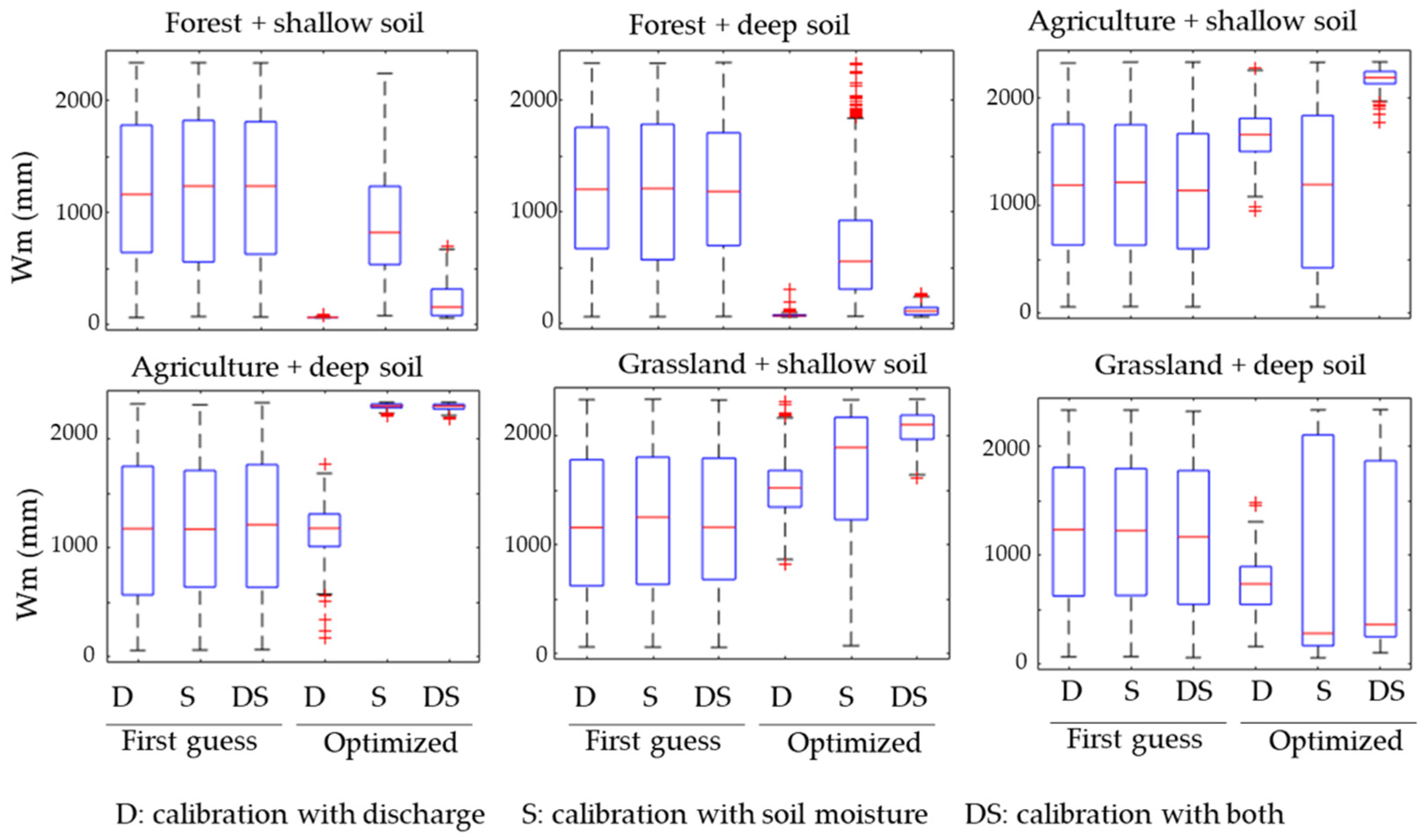
3.3. Estimated Parameter Values

The optimized values of the Wm parameter (maximum soil water storage), which is MGB’s most sensitive parameter, are addressed in this section (Figure 8). The optimization outputs for the other calibrated parameters (b, Kbas, Kint, CS, CI, and CB) are presented in Figures S3–S6, while their optimized behaviors lead to similar conclusions. For most HRUs, the Wm calibration led to narrower optimized ranges for the CAL-DS, followed by CAL-D. The CAL-S scenario led to the most disperse parameter values for most HRUs. For many cases (shallow soil HRUs and forests with deep soils) CAL-D and CAL-DS converged to the same region of the parameter space (i.e., parameter values relatively similar), while for others (e.g., agriculture with deep soil) the CAL-DS converged to similar values as for CAL-S. Furthermore, it is interesting that CAL-DS led to values close to the bottom or top limits of the Wm parameter range, except for grassland with deep soils.

3.4. Number of Adopted Gauges for Calibration

It is paramount in the context of hydrological model calibration to understand the impacts of gauge sampling on the optimization results. Here, a calibration scenario with 136 gauges (G136) was compared to a simpler one where only nine gauges were considered (G9). The sampling of the nine gauge locations was also applied to the CAL-S scenario by using the average upstream soil moisture values for only nine locations in the basin instead of considering 136 locations. Small differences were obtained for model accuracy improvements between G136 and G9 (Figure 9); however, a major gain in the overall performance precision was obtained when considering the large dataset (G136), even when analyzing the same gauge locations used for the calibration (see black circles in Figure 9). A similar conclusion was obtained for the CAL-D and CAL-S scenarios (Figures S8 and S9). It can also be noted that the calibration with nine gauges led to a slightly poorer discharge performance in the south Paraná tributaries, such as the Iguaçu river, where the precipitation is not seasonal, in contrast to the rest of the basin.

4. Discussions

4.1. Combining Discharge and Soil Moisture Data Leads to Optimized Solutions

The largest benefits for model performance were obtained when both discharge and soil moisture data were considered in the calibration. When looking at discharges, this strategy led to the highest overall precision gains in KGE and flow estimates as accurate as those in the calibration scenario with discharge only. Similarly, it resulted in soil moisture estimates as accurate as those obtained in the calibration with soil moisture only. This shows that the calibration acts as a combination of the individual calibrations, since it improved both variables without degrading either of them, i.e., the model was constrained toward more satisfactory estimates. These results are coherent with recent studies [23,60,61]. Calibrating the model with only one data type allows error transference among parameters, and consequently for the model state variables. Constraining the model in different aspects minimizes this type of error.
The larger difficulty of the calibration procedure to estimate soil moisture (which led to more dispersed estimates) may be related to the limited comparability between MGB and SMOS RZSM soil moisture estimates, as the first is associated with a bucket soil with one only layer, while the second with a simple filter used to extrapolate topsoil moisture estimates to the whole root zone profile. In addition, the intrinsic nature of the variables may have also played a role here, since soil moisture is more likely to be variable in time and space, while discharge is an aggregation variable of upstream areas. To overcome this, a typical approach is to rescale the satellite-derived soil moisture to the hydrological model max–min range, as applied in the observation operators in data assimilation [24,62], which was carried out here and which makes the remote sensing observations vary for each new model run in the optimization procedure. These constant changes in the ‘observed’ variable may hinder the calibration algorithm to achieve a more optimal parameter set. The conceptual nature of the MGB model also makes it difficult to draw a conclusion on the link between physical processes and the optimized parameter values and to understand whether the calibration is effectively reducing equifinality. An important limitation of this study is that the soil moisture estimated by the hydrological model and by SMOS were spatially aggregated in the upstream areas of the gauge stations. There are still important questions regarding the mechanisms and factors controlling the spatial distribution of this variable (e.g., Srivastava et al. [63]) and how these automatic calibration strategies are able to capture the related physical processes. Our results, however, confirm that both model accuracy and precision are improved with the combined used of discharge and soil moisture data, which in the context of explicit soil moisture accounting models such as the MGB, suggests a reduction in equifinality by constraining different model state variables. This is in accordance with Nijzing et al. [32], who showed that the combination of multiple datasets such as soil moisture and GRACE total water storage data can help estimate parameters within a narrow parameter search space. Recent studies involving model calibration have also shown the improved water cycle representation when using multiple hydrological variables in combination [33,64].
This study adopted multiobjective functions for both calibrations with individual variables and their combination, which may have helped constrain the model. By using one only variable to define objective functions, errors can be more easily propagated for different model parameters. The use of other variables than discharge and soil moisture is also promising (e.g., evapotranspiration [65,66,67,68] and total water storage [69,70]) for not only estimating the discharge [32,71], but for also improving the model realism [35,64], reducing uncertainty [72,73], and improving the spatial representation of variables [33,74].
Finally, the calibration with 136 gauges reduced to some extent the optimized dispersion in comparison to the scenario with 9 gauges, yet the difference was not very large, meaning the calibration with only a few gauges can be assumed to be satisfactory. This has implications for estimations in poorly gauged basins. For instance, in a more operational scenario, one could use the results of the G9 calibration to estimate the prior parameter sets of the SM-related parameters.
By improving the estimations of water quantity in poorly gauged basins and improving the model realism, this study represents as a potential tool for water resource management, which is linked to the Sustainable Development Goals (SDG) for clean water and sanitation, affordable and clean energy (related to hydropower plants), and life on land, since biodiversity is related to water availability.

4.2. Calibrating a Heterogeneous Large Basin Affected by Anthropogenic Activities

Even though this study focuses on the Upper Paraná Basin, it is worth mentioning that the large extents of the basin encompass characteristics from many catchments worldwide in terms of lithology (permeable sandstones to less permeable basalts), precipitation seasonality (high in the north to low in the south), and irrigation schemes (dense in the north, less dense in the south). Model calibration studies involving remotely sensed soil moisture data are becoming more common for large basins, with examples including the studies by Okavango [18] and Volta [33] in Africa, Quijang and Ganjiang [75] in Asia, Moselle [64] and Rhine-Meuse [23] in Europe, Mississippi [21] in North America, and Purus [35] in South America. Several of these studies covered basins impacted by anthropogenic activities, showing that the exploitation of soil moisture for model calibration or data assimilation improves the model predictability in complex environments; however, the question of the capability of soil moisture to improve the representation of discharges in human-affected basins is still not fully answered. Our results showed that the impacts of irrigated areas on the model calibration outputs were not very relevant; this conclusion may not be applied to basins in semi-arid and arid environments, for which further analyses need to be applied. Basin-wide, the parameters’ values mainly reflected different lithology types and the resulting impact of the geological controls (which varied from sandstones to basalts in the Upper Paraná Basin) on the hydrological regime.

4.3. Uncertainties in MGB and SMOS RZSM

Remote sensing products are limited in spatial and temporal resolution and are subject to a series of error sources. SMOS can be particularly impacted by RFI, which is not very frequent in South America [76]. Furthermore, while L-Band radiometry has a high observation capacity over vegetation cover, it still exhibits saturation over very dense vegetation [77]. The surface roughness, topographic index, water ponding, soil moisture regime, and soil texture are other features that can impact the soil moisture retrievals [78,79]. In turn, the soil water dynamics are usually misrepresented in large-scale hydrological models. Complex models, representing the dynamics between soil moisture and plant growth, require more data and involve larger sets of parameters than simpler water balance models do, often relying on the upscaling of functions developed for local scales (e.g., Richard’s equation). The use of root zone soil moisture estimates is a better match with the soil moisture capacity of the MGB model, although such estimates also have their own limitations. For instance, the SMOS RZSM uses the surface soil moisture data, even though in semi-arid to arid regions the link between surface and root zone soil moisture is weak. Additionally, the empirical approach is based on coarse-resolution texture maps, which can add errors to the estimates; therefore, the use of both types of information combined (remotely sensed and simulated soil moisture) and cross-validation between them is an interesting approach to improve model predictions.
For areas with strongly seasonal precipitation, despite being able to represent the general behavior of soil moisture variations throughout the year, the degree of MGB saturation increases more slowly when the rainy season starts and decreases faster than SMOS RZSM when the dry season arrives. These results reflect a limitation of MGB related to its single soil layer [35]. The implementation of a multilayer approach could reduce the errors associated with a simplified representation of soil water dynamics [80]. Furthermore, the employed model setup does not represent basin-wide anthropogenic impacts as irrigation schemes and reservoirs, and if performed this may especially enhance the representation of river discharges, which are largely affected by reservoirs in its downstream reaches [81]. To overcome this issue, here we have used only in situ river discharge data in non-regulated reaches, while for regulated reaches we have adopted the naturalized flows estimated by ONS.

5. Conclusions

In this study, we have presented large-scale model calibration experiments with distributed in situ discharge and remote sensing soil moisture data from the new SMOS L4 RZSM product. The study area was the Upper Paraná Basin in South America (drainage area > 900,000 km2), the heterogeneity and dimensions of which make its sub-basins equivalent to large basins elsewhere.
While most calibration experiments focus on accuracy improvement, here we moved beyond this and showed the impacts of model calibration on improving not only the accuracy, but also the precision of the estimates (measured in terms of performance precision) across the whole basin. The joint calibration with both discharge and soil moisture data improved the accuracy of both variables to the same level as the calibrations performed individually with each variable and additionally led to more precise estimates, highlighting the benefits of using soil moisture data as additional information to constrain hydrological models.
Regarding the basin heterogeneity, the main factor that led to the different calibrated parameter sets was the lithology type, e.g., the highest precision improvements were obtained for sandstone areas. Furthermore, the choice between a few (9) and many (136) gauges for calibration was also investigated, showing that the calibration with 136 gauges reduced to some extent the optimized dispersion in comparison to the scenarios with 9 gauges, yet the difference was not very large and calibration with only a few gauges is already satisfactory for defining an initial a priori parameter set.
While this was one of the first model calibration experiments involving remotely sensed soil moisture data performed in South America, future studies should move forward and evaluate the added benefits of using other relevant water cycle variables, such as evapotranspiration and total water storage. A better understanding of the uncertainty of the SMOS RZSM product is also necessary, as well as its propagation throughout the hydrological modeling cascade. The recently available high-resolution SMOS-based surface water product [82] may be used in combination with SMOS soil moisture estimates for large river–floodplain systems, which also occur in the La Plata Basin and in South America in general. In this context, coupled hydrologic–hydrodynamic models can be used to better represent the processes occurring in these areas, opening up the possibility for the use of other remote sensing variables (e.g., satellite altimetry and future SWOT observations) to constrain calibrations of hydraulic parameters, such as the ones related to river geometry.

Supplementary Materials

The following are available online at https://www.mdpi.com/article/10.3390/rs13163256/s1. Figure S1. Time series of discharge (upper panel) and soil moisture (bottom panel) for the initial and final calibration generations, for the location of Itaipu dam close to the basin outlet. The calibration with all 136 gauges (G136) and 9 selected gauges (G9) are presented. CALD refers to calibration with discharge only, CALS to calibration with soil moisture only, and CALDS to the joint calibration with both. Given the rescale of SMOS data to the MGB model min/max values, SMOS initial and final generations are different and plotted as green and blue lines, respectively. Figure S2. Relation between drainage area (first row), upstream irrigation areas (second row) and precipitation seasonality index (third row) with overall precision, and accuracy improvement for discharge and soil moisture. Results presented for the scenario of calibration with 136 gauges. In the first row, the maximum drainage area is truncated at 10.000 km2; to improve visualization of most gauges. Figure S3. Initial (ini) and optimized (end) values for the b parameter (unit: adimensional) for the three calibration scenarios (discharge only (D); soil moisture only (S); and calibration with both (DS)) and six HRU’s: (1) Forest with shallow soils; (2) Forest with deep soils; (3) Agriculture with shallow soils; (4) Agriculture with deep soils; (5) Grasslands with shallow soils; and (6) Grasslands with deep soils. “b” is the shape parameter of the ARNO model, which defines the sensitivity of runoff generation on saturated areas. Figure S4. Initial (ini) and optimized (end) values for the Kint parameter (unit in mm.day-1) for the three calibration scenarios (discharge only (D); soil moisture only (S); and calibration with both (DS)) and six HRU’s: (1) Forest with shallow soils; (2) Forest with deep soils; (3) Agriculture with shallow soils; (4) Agriculture with deep soils; (5) Grasslands with shallow soils; and (6) Grasslands with deep soils. This parameter refers to the subsurface flow (i.e., it is a proxy of soil conductivity). Figure S5. Initial (ini) and optimized (end) values for the Kbas parameter (unit in mm.day-1) for the three calibration scenarios (discharge only (D); soil moisture only (S); and calibration with both (DS)) and six HRU’s: (1) Forest with shallow soils; (2) Forest with deep soils; (3) Agriculture with shallow soils; (4) Agriculture with deep soils; (5) Grasslands with shallow soils; and (6) Grasslands with deep soils. This parameter refers to the groundwater flow (i.e., it is a proxy of groundwater conductivity). Figure S6. Initial (ini) and optimized (end) values for the CS, CI and CB parameters (unit in days) for the three calibration scenarios (discharge only (D); soil moisture only (S); and calibration with both (DS)). These parameters refer to the outflow of the three linear reservoirs (i.e., MGB hillslope routing): surface reservoir (CS), intermediate (CI) and baseflow (CB). Figure S7. Soil moisture and discharge KGE values for the nine gauge locations used for the 9-only calibration scenario; results for the 9-only scenario. Figure S8. Spatial assessment of discharge and soil moisture accuracy improvement (∆KGE) and overall precision gain, when calibrating with nine and 136 gauges (including the nine ones). Results are presented for the calibration scenario with discharge only (CAL-D). The circle size refers to the gauge drainage area, and the black open circles are the location of the nine gauges. Figure S9. Spatial assessment of discharge and soil moisture accuracy improvement (∆KGE) and overall precision gain, when calibrating with nine and 136 gauges (including the nine ones). Results are presented for the calibration scenario with soil moisture only (CAL-S). The circle size refers to the gauge drainage area, and the black open circles are the location of the nine gauges.

Author Contributions

A.S.F., A.A.B. and A.M.O. prepared the first draft and designed the experiments. V.A.S. and B.R.C. designed experiments, discussed results, and revised the final manuscript. A.A.B., W.C., R.C.D.d.P., A.R., F.M.F. and P.R.M.P. supervised the study, discussed results, and revised the final manuscript. Y.K. discussed results and revised the final manuscript. All authors have read and agreed to the published version of the manuscript.

Funding

This research was financially supported by the Brazilian National Council for Scientific Research (CNPq) under grant numbers 141161/2017-5 and 201148/2019-6, the CNES-TOSCA-SMOS program, and the Swiss National Science Foundation (SNSF) 186303.

Institutional Review Board Statement

Not applicable.

Informed Consent Statement

Not applicable.

Data Availability Statement

The data that support the findings of this study are available on request from the corresponding author. All datasets used are open data and their availability are acknowledged along the manuscript.

Acknowledgments

The authors would like to thank the Federal University of Rio Grande do Sul (UFRGS) for institutional support, the CATDS CNES iFremer for the availability of the SMOS L3 and L4 products, and three anonymous reviewers for insightful suggestions.

Conflicts of Interest

The authors declare no conflict of interest.

References

  1. Sivapalan, M.; Takeuchi, K.; Franks, S.W.; Gupta, V.K.; Karambiri, H.; Lakshmi, V.; Liang, X.; McDonnell, J.J.; Mendiondo, E.M.; O’Connell, P.E.; et al. IAHS Decade on Predictions in Ungauged Basins (PUB), 2003–2012: Shaping an exciting future for the hydrological sciences. Hydrol. Sci. J. 2003, 48, 857–880. [Google Scholar] [CrossRef] [Green Version]
  2. Hrachowitz, M.; Savenije, H.H.G.; Blöschl, G.; McDonnell, J.J.; Sivapalan, M.; Pomeroy, J.W.; Arheimer, B.; Blume, T.; Clark, M.P.; Ehret, U.; et al. A decade of Predictions in Ungauged Basins (PUB)—A review. Hydrol. Sci. J. 2013, 58, 1198–1255. [Google Scholar] [CrossRef]
  3. Beven, K. A manifesto for the equifinality thesis. J. Hydrol. 2006, 320, 18–36. [Google Scholar] [CrossRef] [Green Version]
  4. Kirchner, J.W. Getting the right answers for the right reasons: Linking measurements, analyses, and models to advance the science of hydrology. Water Resour. Res. 2006, 42. [Google Scholar] [CrossRef]
  5. Balsamo, G.; Agusti-Panareda, A.; Albergel, C.; Arduini, G.; Beljaars, A.; Bidlot, J.; Blyth, E.; Bousserez, N.; Boussetta, S.; Brown, A.; et al. Satellite and In Situ Observations for Advancing Global Earth Surface Modelling: A Review. Remote Sens. 2018, 10, 2038. [Google Scholar] [CrossRef] [Green Version]
  6. Brocca, L.; Ciabatta, L.; Massari, C.; Camici, S.; Tarpanelli, A. Soil moisture for hydrological applications: Open questions and new opportunities. Water 2017, 9, 140. [Google Scholar] [CrossRef]
  7. Jiang, D.; Wang, K. The Role of Satellite-Based Remote Sensing in Improving Simulated Streamflow: A Review. Water 2019, 11, 1615. [Google Scholar] [CrossRef] [Green Version]
  8. Kerr, Y.H.; Waldteufel, P.; Wigneron, J.P.; Delwart, S.; Cabot, F.; Boutin, J.; Escorihuela, M.J.; Font, J.; Reul, N.; Gruhier, C.; et al. The SMOS L: New tool for monitoring key elements ofthe global water cycle. Proc. IEEE 2010. [Google Scholar] [CrossRef] [Green Version]
  9. Entekhabi, D.; Njoku, E.G.; O’Neill, P.E.; Kellogg, K.H.; Crow, W.T.; Edelstein, W.N.; Entin, J.K.; Goodman, S.D.; Jackson, T.J.; Johnson, J.; et al. The soil moisture active passive (SMAP) mission. Proc. IEEE 2010, 98, 704–716. [Google Scholar] [CrossRef]
  10. Beck, H.E.; Pan, M.; Miralles, D.G.; Reichle, R.H.; Dorigo, W.A.; Hahn, S.; Sheffield, J.; Karthikeyan, L.; Balsamo, G.; Parinussa, R.M.; et al. Evaluation of 18 satellite- and model-based soil moisture products using in situ measurements from 826 sensors. Hydrol. Earth Syst. Sci. 2021, 25, 17–40. [Google Scholar] [CrossRef]
  11. Martínez-Fernández, J.; González-Zamora, A.; Sánchez, N.; Gumuzzio, A.; Herrero-Jiménez, C.M. Satellite soil moisture for agricultural drought monitoring: Assessment of the SMOS derived Soil Water Deficit Index. Remote Sens. Environ. 2016, 177, 277–286. [Google Scholar] [CrossRef]
  12. Lopez, T.; Al Bitar, A.; Biancamaria, S.; Güntner, A.; Jäggi, A. On the Use of Satellite Remote Sensing to Detect Floods and Droughts at Large Scales. Surv. Geophys. 2020, 41, 1461–1487. [Google Scholar] [CrossRef]
  13. Souza, A.G.S.S.; Neto, A.R.; Rossato, L.; Alvalá, R.C.S.; Souza, L.L. Use of SMOS L3 soil moisture data: Validation and drought assessment for Pernambuco State, Northeast Brazil. Remote Sens. 2018, 10, 1314. [Google Scholar] [CrossRef] [Green Version]
  14. Wanders, N.; Bierkens, M.F.P.; de Jong, S.M.; de Roo, A.; Karssenberg, D. The benefits of using remotely sensed soil moisture in parameter identification of large-scale hydrological modelss. Water Resour. Res. 2014, 50, 6874–6891. [Google Scholar] [CrossRef] [Green Version]
  15. Yi, L.; Zhang, W.; Li, X. Assessing hydrological modelling driven by different precipitation datasets via the smap soil moisture product and gauged streamflow data. Remote Sens. 2018, 10, 1872. [Google Scholar] [CrossRef] [Green Version]
  16. Parajka, J.; Naeimi, V.; Blöschl, G.; Komma, J. Matching ERS scatterometer based soil moisture patterns with simulations of a conceptual dual layer hydrologic model over Austria. Hydrol. Earth Syst. Sci. 2009, 13, 259–271. [Google Scholar] [CrossRef] [Green Version]
  17. Campo, L.; Caparrini, F.; Castelli, F. Use of multi-platform, multi-temporal remote-sensing data for calibration of a distributed hydrological model: An application in the Arno basin, Italy. Hydrol. Process. 2006, 20, 2693–2712. [Google Scholar] [CrossRef]
  18. Milzow, C.; Krogh, P.E.; Bauer-Gottwein, P. Combining satellite radar altimetry, SAR surface soil moisture and GRACE total storage changes for hydrological model calibration in a large poorly gauged catchment. Hydrol. Earth Syst. Sci. 2011, 15, 1729–1743. [Google Scholar] [CrossRef] [Green Version]
  19. Silvestro, F.; Gabellani, S.; Rudari, R.; Delogu, F.; Laiolo, P.; Boni, G. Uncertainty reduction and parameter estimation of a distributed hydrological model with ground and remote-sensing data. Hydrol. Earth Syst. Sci. 2015, 19, 1727–1751. [Google Scholar] [CrossRef] [Green Version]
  20. López, P.L.; Sutanudjaja, E.H.; Schellekens, J.; Sterk, G.; Bierkens, M.F.P. Calibration of a large-scale hydrological model using satellite-based soil moisture and evapotranspiration products. Hydrol. Earth Syst. Sci. 2017, 21, 3125–3144. [Google Scholar] [CrossRef] [Green Version]
  21. Koppa, A.; Gebremichael, M.; Yeh, W.W.G. Multivariate calibration of large scale hydrologic models: The necessity and value of a Pareto optimal approach. Adv. Water Resour. 2019, 130, 129–146. [Google Scholar] [CrossRef]
  22. Tong, R.; Parajka, J.; Salentinig, A.; Pfeil, I.; Komma, J.; Széles, B.; Kubáň, M.; Valent, P.; Vreugdenhil, M.; Wagner, W.; et al. The value of ASCAT soil moisture and MODIS snow cover data for calibrating a conceptual hydrologic model. Hydrol. Earth Syst. Sci. Discuss. 2020, 25, 1389–1410. [Google Scholar] [CrossRef]
  23. Sutanudjaja, E.H.; Van Beek, L.P.H.; De Jong, S.M.; Van Geer, F.C.; Bierkens, M.F.P. Calibrating a large-extent high-resolution coupled groundwater-land surface model using soil moisture and discharge data. Water Resour. Res. 2014, 50, 687–705. [Google Scholar] [CrossRef]
  24. Lievens, H.; De Lannoy, G.J.M.; Al Bitar, A.; Drusch, M.; Dumedah, G.; Hendricks Franssen, H.J.; Kerr, Y.H.; Tomer, S.K.; Martens, B.; Merlin, O.; et al. Assimilation of SMOS soil moisture and brightness temperature products into a land surface model. Remote Sens. Environ. 2016, 180, 292–304. [Google Scholar] [CrossRef] [Green Version]
  25. Lievens, H.; Reichle, R.H.; Liu, Q.; De Lannoy, G.J.M.; Dunbar, R.S.; Kim, S.B.; Das, N.N.; Cosh, M.; Walker, J.P.; Wagner, W. Joint Sentinel-1 and SMAP data assimilation to improve soil moisture estimates. Geophys. Res. Lett. 2017, 44, 6145–6153. [Google Scholar] [CrossRef]
  26. López López, P.; Wanders, N.; Schellekens, J.; Renzullo, L.J.; Sutanudjaja, E.H.; Bierkens, M.F.P. Improved large-scale hydrological modelling through the assimilation of streamflow and downscaled satellite soil moisture observations. Hydrol. Earth Syst. Sci. 2016, 20, 3059–3076. [Google Scholar] [CrossRef] [Green Version]
  27. Blyverket, J.; Hamer, P.D.; Bertino, L.; Albergel, C.; Fairbairn, D.; Lahoz, W.A. An evaluation of the EnKF vs. EnOI and the assimilation of SMAP, SMOS and ESA CCI soil moisture data over the contiguous US. Remote Sens. 2019, 11, 478. [Google Scholar] [CrossRef] [Green Version]
  28. Tangdamrongsub, N.; Han, S.C.; Yeo, I.Y.; Dong, J.; Steele-Dunne, S.C.; Willgoose, G.; Walker, J.P. Multivariate data assimilation of GRACE, SMOS, SMAP measurements for improved regional soil moisture and groundwater storage estimates. Adv. Water Resour. 2020, 135, 103477. [Google Scholar] [CrossRef]
  29. Khaki, M.; Awange, J. The application of multi-mission satellite data assimilation for studying water storage changes over South America. Sci. Total Environ. 2019, 647, 1557–1572. [Google Scholar] [CrossRef]
  30. Baugh, C.; de Rosnay, P.; Lawrence, H.; Jurlina, T.; Drusch, M.; Zsoter, E.; Prudhomme, C. The impact of smos soil moisture data assimilation within the operational global flood awareness system (GloFAS). Remote Sens. 2020, 12, 1490. [Google Scholar] [CrossRef]
  31. Yang, H.; Xiong, L.; Ma, Q.; Xia, J.; Chen, J.; Xu, C.Y. Utilizing satellite surface soil moisture data in calibrating a distributed hydrological model applied in humid regions through a multi-objective Bayesian hierarchical framework. Remote Sens. 2019, 11, 1335. [Google Scholar] [CrossRef] [Green Version]
  32. Nijzink, R.C.; Almeida, S.; Pechlivanidis, I.G.; Capell, R.; Gustafssons, D.; Arheimer, B.; Parajka, J.; Freer, J.; Han, D.; Wagener, T.; et al. Constraining Conceptual Hydrological Models With Multiple Information Sources. Water Resour. Res. 2018, 54, 8332–8362. [Google Scholar] [CrossRef] [Green Version]
  33. Dembélé, M.; Hrachowitz, M.; Savenije, H.H.G.; Mariéthoz, G.; Schaefli, B. Improving the Predictive Skill of a Distributed Hydrological Model by Calibration on Spatial Patterns With Multiple Satellite Data Sets. Water Resour. Res. 2020, 56. [Google Scholar] [CrossRef]
  34. Massari, C.; Brocca, L.; Tarpanelli, A.; Moramarco, T. Data assimilation of satellite soil moisture into rainfall-runoffmodelling: A complex recipe? Remote Sens. 2015, 7, 11403–11433. [Google Scholar] [CrossRef] [Green Version]
  35. Meyer Oliveira, A.; Fleischmann, A.; Paiva, R. On the contribution of remote sensing-based calibration to model multiple hydrological variables. J. Hydrol. 2020, 597, 126184. [Google Scholar] [CrossRef]
  36. Xu, X.; Tolson, B.A.; Li, J.; Staebler, R.M.; Seglenieks, F.; Haghnegahdar, A.; Davison, B. Assimilation of SMOS soil moisture over the Great Lakes basin. Remote Sens. Environ. 2015, 169, 163–175. [Google Scholar] [CrossRef]
  37. Al Bitar, A.; Kerr, Y.H.; Merlin, O.; Cabot, F.; Wigneron, J.-P. Root Zone Soil Moisture and Drought Index from SMOS. In Proceedings of the IEEE International Geoscience and Remote Sensing Symposium, Frascati, Italy, 1 July 2013. [Google Scholar]
  38. Collischonn, W.; Allasia, D.; da Silva, B.C.; Tucci, C.E.M. The MGB-IPH model for large-scale rainfall-runoff modelling. Hydrol. Sci. J. 2007, 52, 878–895. [Google Scholar] [CrossRef] [Green Version]
  39. Yapo, P.O.; Gupta, H.V.; Sorooshian, S. Multi-objective global optimization for hydrologic models. J. Hydrol. 1998, 204, 83–97. [Google Scholar] [CrossRef] [Green Version]
  40. Al Bitar, A.; Mahmoodi, A. Algorithm Theoretical BASIS Document (ATBD) for the SMOS Level 4 Root Zone Soil Moisture (Version v30_01); Zenodo, 2020; Available online: https://doi.org/10.5281/zenodo.4298572 (accessed on 17 August 2021).
  41. Al Bitar, A.; Mialon, A.; Kerr, Y.H.; Cabot, F.; Richaume, P.; Jacquette, E.; Quesney, A.; Mahmoodi, A.; Tarot, S.; Parrens, M.; et al. The global SMOS Level 3 daily soil moisture and brightness temperature maps. Earth Syst. Sci. Data 2017, 9, 293–315. [Google Scholar] [CrossRef] [Green Version]
  42. Escorihuela, M.J.; Chanzy, A.; Wigneron, J.P.; Kerr, Y.H. Effective soil moisture sampling depth of L-band radiometry: A case study. Remote Sens. Environ. 2010, 114, 995–1001. [Google Scholar] [CrossRef] [Green Version]
  43. Stroud, P. A Recursive Exponential Filter for Time-Sensitive Data. Rep. LAUR 99-573. 1999, p. 131. Available online: https://www.researchgate.net/publication/242230998_A_Recursive_Exponential_Filter_For_Time-Sensitive_Data (accessed on 17 August 2021).
  44. Pontes, P.R.M.; Fan, F.M.; Fleischmann, A.S.; de Paiva, R.C.D.; Buarque, D.C.; Siqueira, V.A.; Jardim, P.F.; Sorribas, M.V.; Collischonn, W. MGB-IPH model for hydrological and hydraulic simulation of large floodplain river systems coupled with open source GIS. Environ. Model. Softw. 2017, 94, 1–20. [Google Scholar] [CrossRef]
  45. Siqueira, V.A.; Paiva, R.C.D.; Fleischmann, A.S.; Fan, F.M.; Ruhoff, A.L.; Pontes, P.R.M.; Paris, A.; Calmant, S.; Collischonn, W. Toward continental hydrologic–hydrodynamic modeling in South America. Hydrol. Earth Syst. Sci. 2018, 22, 4815–4842. [Google Scholar] [CrossRef] [Green Version]
  46. Paiva, R.; Buarque, D.C.; Collischonn, W.; Bonnet, M.P.; Frappart, F.; Calmant, S.; Bulhões Mendes, C.A. Large-scale hydrologic and hydrodynamic modeling of the Amazon River basin. Water Resour. Res. 2013, 49, 1226–1243. [Google Scholar] [CrossRef] [Green Version]
  47. Fleischmann, A.S.; Paiva, R.C.D.; Collischonn, W.; Siqueira, V.A.; Paris, A.; Moreira, D.M.; Papa, F.; Bitar, A.A.; Parrens, M.; Aires, F.; et al. Trade-Offs Between 1-D and 2-D Regional River Hydrodynamic Models. Water Resour. Res. 2020, 56, 56. [Google Scholar] [CrossRef]
  48. Todini, E. The ARNO rainfall-runoff model. J. Hydrol. 1996, 175, 339–382. [Google Scholar] [CrossRef]
  49. Wigmosta, M.S.; Vail, L.W.; Lettenmaier, D.P. A distributed hydrology-vegetation model for complex terrain. Water Resour. Res. 1994, 30, 1665–1679. [Google Scholar] [CrossRef]
  50. Latrubesse, E.M.; Stevaux, J.C.; Sinha, R. Tropical rivers. Geomorphology 2005, 70, 187–206. [Google Scholar] [CrossRef]
  51. Metcalfe, C.D.; Menone, M.L.; Collins, P.; Tundisi, J.G. The Paraná River Basin; Earthscan Series on Major River Basins of the World 2020; Routledge: Abingdon, Oxon, UK; New York, NY, USA, 2020; ISBN 9780429317729. [Google Scholar]
  52. Beck, H.E.; Van Dijk, A.I.J.M.; Levizzani, V.; Schellekens, J.; Miralles, D.G.; Martens, B.; De Roo, A. MSWEP: 3-hourly 0.25° global gridded precipitation (1979–2015) by merging gauge, satellite, and reanalysis data. Hydrol. Earth Syst. Sci. 2017, 21, 589–615. [Google Scholar] [CrossRef] [Green Version]
  53. CGIAR SRTM 90 m DEM Digital Elevation Database. Available online: https://srtm.csi.cgiar.org/ (accessed on 17 August 2021).
  54. Fan, F.; Buarque, D.C.; Pontes, P.R.M.; Collischonn, W. Um mapa de unidades de resposta hidrológica para a América do Sul. In Proceedings of the Anais do XXI Simpósio Brasileiro de Recursos Hídricos, Brasilia, Brazil, 22–27 November 2015; ABRH: Brasília, Brazil, 2015; p. PAP019919. [Google Scholar]
  55. Farr, T.; Rosen, P.; Caro, E.; Crippen, R.; Duren, R.; Hensley, S.; Kobrick, M.; Paller, M.; Rodriguez, E.; Roth, L.; et al. The shuttle radar topography mission. Rev. Geophys. 2007, 45. [Google Scholar] [CrossRef] [Green Version]
  56. Duan, Q.; Sorooshian, S.; Gupta, V. Effective and efficient global optimization for conceptual rainfall-runoff models. Water Resour. Res. 1992, 28, 1015–1031. [Google Scholar] [CrossRef]
  57. Gupta, H.V.; Kling, H.; Yilmaz, K.K.; Martinez, G.F. Decomposition of the mean squared error and NSE performance criteria: Implications for improving hydrological modelling. J. Hydrol. 2009, 377, 80–91. [Google Scholar] [CrossRef] [Green Version]
  58. ANA. Atlas Irrigação: Uso da Água na Agricultura Irrigada; Agência Nacional de Águas: Brasília, Brazil, 2017.
  59. Walsh, R.P.D.; Lawler, D.M. Rainfall seasonality: Description, spatial patterns and change through time. Weather 1981, 36, 201–208. [Google Scholar] [CrossRef]
  60. Kunnath-Poovakka, A.; Ryu, D.; Renzullo, L.J.; George, B. The efficacy of calibrating hydrologic model using remotely sensed evapotranspiration and soil moisture for streamflow prediction. J. Hydrol. 2016, 535, 509–524. [Google Scholar] [CrossRef]
  61. Rajib, M.A.; Merwade, V.; Yu, Z. Multi-objective calibration of a hydrologic model using spatially distributed remotely sensed/in-situ soil moisture. J. Hydrol. 2016, 536, 192–207. [Google Scholar] [CrossRef] [Green Version]
  62. De Lannoy, G.J.M.; Reichle, R.H. Assimilation of SMOS brightness temperatures or soil moisture retrievals into a land surface model. Hydrol. Earth Syst. Sci. 2016, 20, 4895–4911. [Google Scholar] [CrossRef] [Green Version]
  63. Srivastava, A.; Saco, P.M.; Rodriguez, J.F.; Kumari, N.; Chun, K.P.; Yetemen, O. The role of landscape morphology on soil moisture variability in semi-arid ecosystems. Hydrol. Process. 2021, 35, e13990. [Google Scholar] [CrossRef]
  64. Demirel, M.C.; Özen, A.; Orta, S.; Toker, E.; Demir, H.K.; Ekmekcioğlu, Ö.; Tayşi, H.; Eruçar, S.; Sağ, A.B.; Sari, Ö.; et al. Additional value of using satellite-based soil moisture and two sources of groundwater data for hydrological model calibration. Water 2019, 11, 2083. [Google Scholar] [CrossRef] [Green Version]
  65. Immerzeel, W.W.; Droogers, P. Calibration of a distributed hydrological model based on satellite evapotranspiration. J. Hydrol. 2008, 349, 411–424. [Google Scholar] [CrossRef]
  66. Becker, R.; Koppa, A.; Schulz, S.; Usman, M.; aus der Beek, T.; Schüth, C. Spatially distributed model calibration of a highly managed hydrological system using remote sensing-derived ET data. J. Hydrol. 2019, 577. [Google Scholar] [CrossRef]
  67. Rajib, A.; Evenson, G.R.; Golden, H.E.; Lane, C.R. Hydrologic model predictability improves with spatially explicit calibration using remotely sensed evapotranspiration and biophysical parameters. J. Hydrol. 2018, 567, 668–683. [Google Scholar] [CrossRef]
  68. Srivastava, A.; Sahoo, B.; Raghuwanshi, N.S.; Singh, R. Evaluation of Variable-Infiltration Capacity Model and MODIS-Terra Satellite-Derived Grid-Scale Evapotranspiration Estimates in a River Basin with Tropical Monsoon-Type Climatology. J. Irrig. Drain. Eng. 2017, 143, 04017028. [Google Scholar] [CrossRef] [Green Version]
  69. Werth, S.; Güntner, A. Calibration analysis for water storage variability of the global hydrological model WGHM. Hydrol. Earth Syst. Sci. 2010, 14, 59–78. [Google Scholar] [CrossRef] [Green Version]
  70. Rakovec, O.; Kumar, R.; Attinger, S.; Samaniego, L. Improving the realism of hydrologic model functioning through multivariate parameter estimation. Water Resour. Res. 2016, 52, 7779–7792. [Google Scholar] [CrossRef]
  71. Huang, Q.; Qin, G.; Zhang, Y.; Tang, Q.; Liu, C.; Xia, J.; Chiew, F.H.S.; Post, D. Using Remote Sensing Data-Based Hydrological Model Calibrations for Predicting Runoff in Ungauged or Poorly Gauged Catchments. Water Resour. Res. 2020, 56. [Google Scholar] [CrossRef]
  72. Zink, M.; Mai, J.; Cuntz, M.; Samaniego, L. Conditioning a Hydrologic Model Using Patterns of Remotely Sensed Land Surface Temperature. Water Resour. Res. 2018, 54, 2976–2998. [Google Scholar] [CrossRef]
  73. Schattan, P.; Schwaizer, G.; Schöber, J.; Achleitner, S. The complementary value of cosmic-ray neutron sensing and snow covered area products for snow hydrological modelling. Remote Sens. Environ. 2020, 239, 111603. [Google Scholar] [CrossRef]
  74. Koch, J.; Demirel, M.C.; Stisen, S. The SPAtial EFficiency metric (SPAEF): Multiple-component evaluation of spatial patterns for optimization of hydrological models. Geosci. Model. Dev. 2018, 11, 1873–1886. [Google Scholar] [CrossRef] [Green Version]
  75. Xiong, L.; Zeng, L. Impacts of introducing remote sensing soil moisture in calibrating a distributed hydrological model for streamflow simulation. Water 2019, 11, 666. [Google Scholar] [CrossRef] [Green Version]
  76. Oliva, R.; Daganzo, E.; Kerr, Y.H.; Mecklenburg, S.; Nieto, S.; Richaume, P.; Gruhier, C. SMOS Radio Frequency Interference Scenario: Status and Actions Taken to Improve the RFI Environment in the 1400–1427-MHz Passive Band. IEEE Trans. Geosci. Remote Sens. 2012, 50, 1427–1439. [Google Scholar] [CrossRef] [Green Version]
  77. Parrens, M.; Wigneron, J.P.; Richaume, P.; Mialon, A.; Al Bitar, A.; Fernandez-Moran, R.; Al-Yaari, A.; Kerr, Y.H. Global-scale surface roughness effects at L-band as estimated from SMOS observations. Remote Sens. Environ. 2016, 181, 122–136. [Google Scholar] [CrossRef]
  78. Al Bitar, A.; Leroux, D.; Kerr, Y.H.; Merlin, O.; Richaume, P.; Sahoo, A.; Wood, E.F. Evaluation of SMOS Soil Moisture Products Over Continental U.S. Using the SCAN/SNOTEL Network. IEEE Trans. Geosci. Remote Sens. 2012, 50, 1572–1586. [Google Scholar] [CrossRef] [Green Version]
  79. Gumuzzio, A.; Brocca, L.; Sánchez, N.; González-Zamora, A.; Martínez-Fernández, J. Comparison of SMOS, modelled and in situ long-term soil moisture series in the northwest of Spain. Hydrol. Sci. J. 2016, 61, 2610–2625. [Google Scholar] [CrossRef] [Green Version]
  80. Guimberteau, M.; Ducharne, A.; Ciais, P.; Boisier, J.P.; Peng, S.; De Weirdt, M.; Verbeeck, H. Testing conceptual and physically based soil hydrology schemes against observations for the Amazon Basin. Geosci. Model. Dev. 2014, 7, 1115–1136. [Google Scholar] [CrossRef] [Green Version]
  81. Fleischmann, A.S.; Brêda, J.P.F.; Passaia, O.A.; Wongchuig, S.C.; Fan, F.M.; Paiva, R.C.D.; Marques, G.F.; Collischonn, W. Regional scale hydrodynamic modeling of the river-floodplain-reservoir continuum. J. Hydrol. 2021, 596, 126114. [Google Scholar] [CrossRef]
  82. Parrens, M.; Al Bitar, A.; Frappart, F.; Paiva, R.; Wongchuig, S.; Papa, F.; Yamasaki, D.; Kerr, Y. High resolution mapping of inundation area in the Amazon basin from a combination of L-band passive microwave, optical and radar datasets. Int. J. Appl. Earth Obs. Geoinf. 2019, 81, 58–71. [Google Scholar] [CrossRef]
Figure 1. Flow chart of the study methodology.
Remotesensing 13 03256 g001
Figure 2. The Upper Paraná River Basin in South America. The 136 river gauges used are presented as green circles or highlighted as purple circles for nine gauges of interest. The location of the Itaipu dam is also presented.
Remotesensing 13 03256 g002
Figure 3. Illustrative scatterplot of initial and optimized sets of KGE values for a hypothetical gauge, explaining the accuracy (∆KGED and ∆KGES) and precision ( Dist ini ¯   /   Dist end ¯ ) improvement metrics. The initial and optimized sets contain 500 individuals each.
Remotesensing 13 03256 g003
Figure 4. Spatial assessment of 136 gauges for overall performance precision gain (i.e., the joint improvement in precision of soil moisture and discharge) (first row) and accuracy improvement for discharge (second row) and soil moisture (third row) data for the calibration scenarios involving discharge only (first column; CAL-D), soil moisture only (second column; CAL-S), and the combination of both (third row; CAL-DS). The circle size refers to the gauge drainage area, while the maximum circle size is limited for drainage areas > 10,000 km2.
Remotesensing 13 03256 g004
Figure 5. Soil moisture and discharge KGE values for initial and optimized solutions at nine selected gauge locations when calibrated with 136 river gauges (see the locations of all 136 gauges in Figure 2). The upstream drainage area (km2) for each gauge is also presented. Each set of points refer to one calibration scenario (with soil moisture, discharge, and both).
Remotesensing 13 03256 g005
Figure 6. Assessment of accuracy improvements for discharge and soil moisture parameters for the six lithology types and three calibration scenarios (with discharge, with soil moisture, and with both). Each boxplot refers to one lithology type.
Remotesensing 13 03256 g006
Figure 7. Performance precision improvements according to (a) geological characteristics (six lithology classes), (b) water use for agriculture (irrigation areas, divided into three groups of irrigation areas—most irrigated, intermediate, and least irrigated upstream areas), and (c) precipitation characteristics (seasonality, divided into three groups—high, intermediate and low seasonality in upstream areas). In the second and third rows of maps, each point refers to one of the 136 gauge locations used for the model calibration. Each boxplot refers to a different class (geological characteristics, irrigation areas and precipitation seasonality).
Remotesensing 13 03256 g007
Figure 8. Ranges of Wm parameter (maximum soil water storage) values for the initial first guess and the optimized sets.
Remotesensing 13 03256 g008
Figure 9. Spatial assessment of discharge and soil moisture accuracy improvements (∆KGE) and overall precision gain when performing calibrations with nine and 136 gauges. The results are presented for the calibration scenario with both discharge and soil moisture (CAL-DS), while the results for CAL-D and CAL-S scenarios are shown in Supplementary Figures S8 and S9. The circle size refers to the gauge drainage area, while the black open circles are the locations of the nine gauges. A maximum circle size is limited for drainage areas > 10,000 km2.
Remotesensing 13 03256 g009
Table 1. Input data used in this study.
InformationData Source
Precipitation0.1° daily precipitation from MSWEP 2.1 [52]
Climatic variables (surface temperature, relative humidity, solar radiation, wind speed, atmospheric pressure)INMET stations (195 gauges)
HRU classes (combination of land use and soil types)South America HRU map (400 m) [54]
Digital elevation modelSRTM v4 (90 m) [55]
Remotely sensed soil moistureSMOS L4 Root Zone Soil Moisture (RZSM) product (25 km) [40]
Observed dischargeANA in situ discharges and ONS naturalized flows (136 in situ gauges) (snirh.gov.br/hidroweb/)
Table 2. Reference values for the a priori distribution (initial guess) of MGB parameters for each HRU (except for CS, CI, and CB parameters, which were constant for the whole basin), derived from the average values of the MGB model application for South America [45]. Each initial set of parameters (total of 500 sets for each of the three calibration scenarios) was obtained by estimating the parameter values with a uniform distribution within a range of 10% to 400% of the reference value defined by this table.
ParameterReference Value
Wm (maximum water storage capacity in the soil) [mm]585
b (parameter related to variable infiltration curve) [-]0.26
Kbas (percolation rate from soil to groundwater) [mm·day−1]0.65
Kint (saturated hydraulic conductivity) [mm·day−1]9.48
Cs (adjustment factor for surface linear reservoir residence time) [day]15.6
Ci (adjustment factor for subsurface linear reservoir residence time) [day]105.7
Cb (groundwater reservoir residence time) [day]2547.0
Publisher’s Note: MDPI stays neutral with regard to jurisdictional claims in published maps and institutional affiliations.

