Abstract
The increased development of camera resolution, processing power, and aerial platforms helped to create more cost-efficient approaches to capture and generate point clouds to assist in scientific fields. The continuous development of methods to produce three-dimensional models based on two-dimensional images such as Structure from Motion (SfM) and Multi-View Stereopsis (MVS) allowed to improve the resolution of the produced models by a significant amount. By taking inspiration from the free and accessible workflow made available by OpenDroneMap, a detailed analysis of the processes is displayed in this paper. As of the writing of this paper, no literature was found that described in detail the necessary steps and processes that would allow the creation of digital models in two or three dimensions based on aerial images. With this, and based on the workflow of OpenDroneMap, a detailed study was performed. The digital model reconstruction process takes the initial aerial images obtained from the field survey and passes them through a series of stages. From each stage, a product is acquired and used for the following stage, for example, at the end of the initial stage a sparse reconstruction is produced, obtained by extracting features of the images and matching them, which is used in the following step, to increase its resolution. Additionally, from the analysis of the workflow, adaptations were made to the standard workflow in order to increase the compatibility of the developed system to different types of image sets. Particularly, adaptations focused on thermal imagery were made. Due to the low presence of strong features and therefore difficulty to match features across thermal images, a modification was implemented, so thermal models could be produced alongside the already implemented processes for multispectral and RGB image sets.
1. Introduction
Technological growth experienced in the last decades allowed for improved computational power, consequence of the increase number of transistors integrated on circuits, which in turn also assisted on the increase in product quality over the years. Additionally, due to the complexity and energy demands of electrical circuits, progress were made to improve component’s energy efficiency in order to lower the overall impact of energy product in the environment. This way, a path was paved that led to an improvement in storage capacity and growth in image quality through the increase availability of more pixels in cameras [1].
The image collection obtained from an aerial survey is embedded with information regarding the camera’s configurations, most notably its distortion coefficients, and in some cases, where aerial vehicles are followed with a locating device, the information related to Global Navigation Satellite System (GNSS) coordinates and vehicle’s attitude can be relayed to the camera and stored in the metadata of the image file.
From the information extracted from the metadata of the image set, the algorithm analyzes and withdraws features of each image and compares them between neighboring images using the SIFT [2] and FLANN [3] methods, respectively. On the later method, image pairings are created indicating that features on one image were present on the other. Feature tracks are created using this image pairing information. The tracks inform how the feature was developed over the course of the survey and what are the images present on each feature track. Finally, the reconstruction is built using incremental reconstruction by iteratively adding images to the overall model until no more images of the image set are left. The steps described above compose the Structure from Motion (SfM) workflow.
As the previous workflow produces a point cloud model with a low point density, the resolution is greatly reduced. This way, a densification process is performed by estimating and merging depth maps using the images that were integrated into the sparse point cloud. From this, a higher density of points is obtained with improved resolution. Afterward, a mesh surface is created and textured using the image collection.
The extracted GNSS information from the metadata of each image is used to locate geographically the reconstructed model in the real world reference, and finally, an orthomap of the surveyed area is created.
Furthermore, image metadata information alongside the flexibility that UAVs possess creates a fast-expanding field in remote sensing where georeferenced and high-resolution models such as orthomaps, digital surface/elevation models, and point clouds can be used as assessment tools of remote sensing.
In addition, on the writing of this paper, no literature was found that addresses in detail the processes taken to generate a map from aerial images obtained using an unmanned aerial vehicle (UAV). Therefore, and by taking inspiration on the workflow of [4], this paper aims to reveal an overview of an automated system that allows the creation of maps using aerial images. Moreover, an analysis of the details on why each step was taken and how ultimately 3D models are produced is performed.
Additionally, from the study of the developed system, it was observed that no thermal imaging implementation was integrated. Moreover, literature research showed that mapping thermal images usually presents low resolution. This is due to homogeneity of outdoor environments and the low presence of features in thermal images, so thermal images are captured at higher altitudes, increasing the camera’s footprint, while lowering resolution. This way, a different approach was considered, and an open-source method was proposed that allowed thermal images to be used by the implemented mapping technique.
The paper is comprised of the current introduction, a state of art of structure from motion is studied in Section 2. Section 3 represents the core of this paper and is composed by the steps of the system. For each step, an introduction to its objective is made followed by a detailed analysis of the implemented approach. In order to illustrate the products derived from each step, their output models are presented. Section 4 presents the results obtained using different data sets processed using the automated system. Lastly, a conclusion and remarks are made in the final section.
2. Related Work
Photogrammetry is a mapping method often used in the production of accurate digital reconstruction of physical characteristics such as objects, environment, and terrain through the documentation, measurement, and interpretation of photographic images. It is a process used to deduce the structure and position of an object from aerial images through image measurements and interpretation. The goal of these measurements is to reconstruct a digital 3D model by extracting three-dimensional measurements from two-dimensional data.
The process of photogrammetry is similar to how a human’s eye percepts depth. Human eyes are based on the principle of parallax, and it refers to the effects of changing the perspective regarding a stationary object. A common point on each image is identified, and a line of sight (or ray) is constructed between the camera and these points. The intersection of two or more rays enables the ability to obtain a 3D position of the point using triangulation. Repeating this process to every point corresponding to a surface can be used to generate a Digital Surface Model (DSM).
The improvement of sensors and data acquisition devices along with advances to surveying platforms which increased the use of UAVs in field surveys lead to an improvement in resolution of orthomaps and point clouds using the photogrammetry technique.
As the demand of software that was able to process images and create digital models to be used in scientific fields increased, two categories of programs were developed: commercial and free.
The commercial programs provide the needed photogrammetry functionalities at a cost, usually in bundles based on the customer’s needs. Two widely known programs in the sphere of computer vision photogrammetry are Agisoft and Pix4D.
Agisoft Metashape is a computer vision software developed and commercialized by Agisoft LLC. and is used to produce quality digital models and orthomosaics. It allows the processing of RGB and multispectral images with the ability to eliminate shadows and texture artifacts as well as compute vegetation indices. Metashape also allows the combination of SfM with laser scanning surveying techniques in order to increase the quality of digital models [5].
Pix4D is a software company that develops a photogrammetry program. It allows the automatic computation of image orientation and block adjustment technology to calibrate images. A precision report is returned by the program containing detailed information regarding automatic aerial triangulation, adjustments, and GCP accuracy to assess the quality of the generated model [6].
Nevertheless, often the cost to acquire such commercial programs is a constraint for surveyors. Therefore, open-source programs developed and made accessible by community users are an alternative. However, as these are developed by users’ contributions, these are usually simpler programs that lack some or most of the functionalities available compared to commercial ones. On the other hand, as these programs are open-sourced, users can customize, make adjustments, or even develop their own improvements in an attempt to optimize and further develop the general concept of SfM and make them available for future users to benefit from. Examples of some free photogrammetric programs are Microsoft Photosynth, Arc3D, and Bundler.
Arc3d stands for Automatic Reconstruction Conduit to generate 3d point clouds and mesh surfaces, and it is available as a web service. It possesses tools to produce and visualize digital models derived from user-inputted data. The service performs calibration, feature detection, and matching as well as a multi stereo reconstruction over a distributed network producing at the end a dense point cloud as a result and making the process faster and more robust [7].
Bundler is a free program developed based on the technique of SfM. It was used as a method of reconstruction using unordered image collections. Bundler operated similarly as SfM, but the reconstruction was done incrementally. However, Bundler is unable to develop dense point clouds so a complementing program is needed to help densify the point clouds, PMVS2 (Patch-based Multi-view Stereo Software version 2) [8].
In order to evaluate the performance of both commercial and free software, the results studied in literature and obtained by other authors are shown ahead.
In [9], software-based in SfM were evaluated based on the effects on accuracy, ground sampling distance (GSD), and horizontal and vertical accuracy, depending on the ratio of GCPs vs checkpoints (CP), and the relation to its distribution.
In this work, Agisoft Metashape, Inpho UAS Master, Pix4D, ContextCapture and MicMac were evaluated by their performance.
Inpho UAS Master is a software developed and sold by Trimble. It allows the production of point clouds through imaging as an alternative to laser scans with help of geo-referencing and calibration. Ability to create colorized digital models and orthophotos.
Context Capture developed by Bentley aims to produce 3d models derived from physical infrastructures from photographs in as a small time frame as possible. The 3D models generated by it enable users to obtain a precise real-world digital context to aid in decision-making.
MicMac is a free open-source photogrammetric software with contributions from professionals and academic users in order to provide constant improvements. A benefit of this method of development is the high degree of versatility which can be useful in different kinds of study fields.
Three configurations were set up, one for control with 18 GCPs used for camera calibration, and the result of two configurations were tested against the control one. One test configuration used 11 GCPs and 7 CPs and the other one 6 GCPs and 12 CPs. The configurations are illustrated in Figure 1.
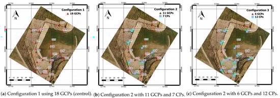
Figure 1.
Configurations used to evaluate the effects of GCPs distribution and GCP vs CP relation: (a) is used as a control group as all the markers are used as GCPs; (b) illustrates the second configuration where the markers are split into two types, GCPs and CPs, where 12 markers are used as GCPs and 7 for CPs, respectively. The final image (c) aims to evaluate the results obtained by using less markers as GCPs. Adapted from [9].
Aside from ContextCapture, all three software performed delivered results below the GSD which was calculated to be around 1.8 cm.
Agisoft and MicMac were further selected to evaluate the effects of the distribution and amount of GCPs using Leave-one-out (LOO) cross-validation. These programs were chosen based on their performance, and the first configuration was chosen because it had evenly distributed GCPs.
In this case, one GCP was left out of the bundle adjustment process and later tested. The objective of this assessment was to verify if a particular GCP can influence the final result. The errors present in this assessment did not provide a significant deviation from the previous test, and a conclusion was reached as the GCP configuration did not play a part in the results obtained by the previous test. The values of the experiment are displayed in Table 1.

Table 1.
Results obtained from the different software tested. Adapted from [9].
A couple of different programs were compared in [10]. A previously tested Agisoft was compared along with Microsoft Photosynth, ARC3D, bundler, and CMVS/PMVS2 in terms of point cloud quality.
From the beginning, a deduction could be reached regarding point cloud completeness. Agisoft presented a complete point cloud without any gaps with 1.3 million points followed by PVMS2 with 1.4 million points although it presents gaps in some zones. The pair Photosynth and Bundler presented similar results with a point cloud with several gaps. ARC3D presented the worst results from the fact that it was only capable of generating point clouds using half of the coverage resulting in regions with high point density but with the presence of void patches. Figure 2 illustrates the results obtained.
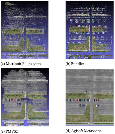
Figure 2.
Comparison of different programs. (a) point cloud produced by Microsoft Photosynth. Several gaps are present in the point cloud. Features (cars) are barely visible; (b) Bundler’s point cloud presents similar results as (a). Gaps are present as well as barely detectable features; (c) PMVS2 presents a clearer cloud compared to (a,b). The point cloud is almost complete except for the edges and at the center. In this case, the cars are very distinguishable; (d) Agisoft Metashape produced a complete point cloud with no gaps. Adapted from [10].
A later accuracy test was performed using the two best-performing programs, Agisoft and PVMS2, to estimate their point cloud accuracy. Because the same dataset was used on both programs, this was used to estimate the accuracy of each program. It was noted that for both programs, the positional accuracy presented roughly the same amount of deviations. From PMVS2 resulted a deviation of 235 mm for the entire area and 136 mm for nearby points of the referenced markers while Agisoft presented deviations of 256 mm and 56 mm, respectively. Regarding height deviations, points generated using PMVS2 presented themselves, on average, with a 5 mm deviations for the complete survey area and 2 mm deviations near referenced markers. In contrast, Agisoft generated points displayed −5 mm of height deviations when the complete area was assessed and −25 mm close to GCPs. Additionally, Agisoft seemed to keep a stable deviation compared to PMVS2 which seemed to degrade near the edges. Figure 3 illustrates the results obtained from the positional and height accuracy.
In [11] a comparison of standard photogrammetry programs and computer vision software was made. Concepts should be clarified here. In the literature, programs in which user input is required, except for image dataset introduction, are classified as standard photogrammetry. In contrast, computer vision software is a program that given the image dataset can identify feature points, align images in a specific orientation, perform georeferencing, self-calibrate, and produce a point cloud without any user interaction besides settings configuration/optimization.

Figure 3.
Positional and height deviations comparisons between the results obtained from PMVS2 and Agisoft. The vectors illustrated on the (a,c) represent the deviations in position of points. Larger vector sizes indicate a larger deviation. The circles on (b,d) describe the height deviations of points, where larger circles represent larger height deviations. Additionally, the crosses illustrate reference markers. Adapted from [10].

Here, Erdas Leica Photogrammetry Suite (LPS), Photomodeler Scanner (PM), and EyeDEA were analyzed as photogrammetry programs. Agisoft Metashape and Pix4d were compared as computer vision software.
The first difference between these programs was the ability to detect GCPs. LPS and EyeDEA needed manual selection while Pix4d and Agisoft were able to detect GCPs automatically. The effect of this is the deviations later obtained in the bundle block adjustments are smaller on computer vision software when compared to photogrammetry programs.
Digital Surface Models (DSM) were also used to compare the software. Agisoft was able to recognize edges and produced a sharper DSM while the other programs had to interpolate values in areas where sharp height variation occurred.
To conclude, the authors point out that photogrammetry programs obtained the best Root Mean Square Error (RMSE) of control points as photogrammetry’s RMSE are 2–4× lower than the RMSE presented by computer vision software. This fact could be explained by the manual selection of control points compared to computer vision. The RMSE values are displayed in Table 2.
Table 2.
CP RMSE values obtained for each software. Adapted from [11].
However, computer vision software’s ability to automatically generate dense point clouds such as Agisoft seemly achieved the most reliable results with lower RMSE and sharper models. This last characteristic is due to height variations being easily identified by Agisoft as edges compared to the other software. Additionally, Agisoft was able to extract features from smooth areas, where it can be harder to identify, and in regions obscured by shadows.
Another work comparison was made in [12] where an orthomap product from Agisoft Metashape was compared to Pix4D. The processing time was calculated, and the accuracy of the orthomaps was computed. The authors reached the conclusion that Agisoft produced orthographic images of the survey area faster, but Pix4D produced a more accurate orthomap.
In [13], a rockfall point cloud was generated and evaluated for its quality. The programs used in this work are Agisoft Metashape and OpenMGV complemented by OpenMVS. This work is important because it reflects the importance of programs to produce accurate point clouds in challenging environments where GPCs placements are not available, so it relies on positional and orientation sensors for georeferencing. These point cloud models were assessed subjectively and objectively based on their model quality and accuracy.
Subjective evaluation is fulfilled by users that classify the completeness, density, and smoothness of the reconstruction. In contrast, objective evaluation measures the accuracy metrics such as the number of points, point density, and point to point distance.
Results from this work showed that for a significantly small area, aerial photogrammetry can produce spatial resolution point clouds with a significantly lower cost and labor compared to traditional laser scanning.
Even though a wide range of programs was presented in this study and their benefits were compared with each other, progressive work has been made to integrated data acquired by UAV with web service solutions.
Guimarães et al. [14] proposed a visual web platform designed to process UAV acquired images based on open-source technologies. The integration of software was done by a client and server using REST communication architecture. This way, information regarding point cloud production settings would be set by users with the images and sent as a request to a server. Here, MicMac would process the image data based on the user’s settings. The result will then be stored on a server and it would be shared with the user via a web application, like Potree [15,16].
The workflow of the platform can be divided into 4 modules. The first module processes the images derived from the UAV survey and returns a map composed by the stitching of individual images and a 3D dense point cloud. Module 2 transfers the orthomosaic to a server making it available to web services. Visualization of the orthomosaic is made possible through the use of a Web Map Service (WMS) responsible for Module 3. The analysis and visualization of the dense point cloud were implemented with leaflet [17] and Potree on the last Module. The Table 3, on the next page, illustrates the errors obtained by each of the programs studied in their works.
Table 3.
A table with the error resulting from the comparison of different programs. Casella et al. and Sona et al. first configuration is used as a control configuration to calibrate the system. The next configurations are used to test different amount of GCP configurations using checkpoints as evaluating points. It is worth noting that Metashape allows a creation of a better fit of data model (lower RMSE values) although with a more balanced amount of GCP/CP (such as config 2 of Casella et al.), MicMac should be mentioned providing less error at the Z component as an open-source web program. In Guimarães et al., errors are quite similar between the two programs surveyed from two study areas.
3. Methodology
In this section, the adopted workflow, inspired by the work of [4], describes the steps and details of how models and orthophotos are reconstructed based on imagery of the surveyed area. A general flowchart that illustrates the steps taken, from the input of image sets to the output of reconstruction models and ortho map, is illustrated in Figure 4
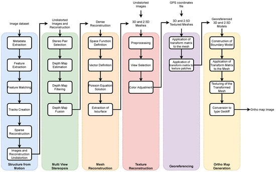
Figure 4.
Step-by-step representation of the methodology implemented.
3.1. Data Load/Input
The images obtained from the survey are then loaded from the camera into the computer and later to the program. Depending on multiple factors, area of survey, overlap level, number of surveys, the program might need to process a high volume of images. In order to optimize this issue, the program takes into account the number of processing cores made available by the system and uses them to process operations in parallel.
A database of the images are created, images.json. This file contains information pertaining to the filename, size of each image, camera make and model, its GNSS coordinates, its band name and index, radiometric calibration, exposure time, and the attitude of the UAV when the image was taken of all the images that compose the dataset.
A list image_list.txt with the path to all the images is created. A coordinate file, coords.txt, is created containing the GNSS positions of all images.
The MicaSense camera, with the GNSS and DLS modules, stores information regarding what type of grid coordinate was used, what world geodetic system was chosen, the unit of measurement adopted, and the coordinate reference system. This information is extracted from the coords.txt file and stored in a proj.txt file.
To georeference the images, a standard coordinate must be declared first. The standard coordinates will establish the geographic positions of a map. Common grid coordinates are UTM, MGRS, USNG, GARS, GEOREF, and UPS.
The world geodetic system (WGS) is the norm used in cartography and satellite navigation that defines geospatial information based on the global reference system. The scheme WGS84 is the reference coordinate system used by the GNSS which best describes the Earth’s size, shape, gravity, and geomagnetic fields with its origin being the Earth’s center of mass [18].
The unit of measurement adopted relates to the magnitude of the distance. In this case, the unit of measurement used is the meters.
The spatial reference system (SRS) or coordinate reference system (CRS) tells the mapping software what method should be used to project the map in the most geographic correct space.
3.2. Structure from Motion
Structure from Motion will be responsible for the sparse reconstruction. Here the images taken from the survey will be processed and a first model will be created.
From each image of the image set, its metadata will be extracted, a database of features detected from each image will be created to be later used to identify similar features in subsequent images. A tracking model will be generated from the feature matching. This tracking model will let the algorithm know the best way to overlap and display the images so a positional agreement can be reached when the map can be generated. Finally, the point cloud model is reconstructed based on the tracking model. Following the tracking model, images are gradually added until no more images are left.
The steps explained below were performed with the assistance of an open-source library available in [4,19].
3.2.1. Metadata Extraction
In this step, the file image_list.txt is used to locate and extract the metadata from the images. This is embedded in the image file at the moment of the capture. An EXIF file is created for each image with the contents of its metadata. It will extract the make and model of the camera used to capture it, size of the image, the projection type used, the orientation and GNSS coordinates of the drone when the image when taken, capture time, focal ratio, and the band name specifying to which multispectral cameras is the image associated with.
Alongside the metadata extraction, the camera settings used at the time of the survey are stored in camera_models.json, that is, information such as the projection type, image size, focal length in the x and y-axis, optical center, k coefficients which correspond to the radial components of the distortion model, and p coefficients (p1 and p2) associated with the tangential distortion components [20].
The measurement of these distortion components is important as the presence of these distortions has an impact on the image texture. If the distortion is not removed, the corners and margins of the image would present a narrower field of view when compared to an undistorted image [21].
Additionally, information regarding the GNSS coordinates and the capture time of each image allows a restriction on the number of images whose features need to be matched against a fewer number of neighboring images [18].
3.2.2. Feature Detection
In this step, features are extracted from each image, and a database is created with this information.
Published in 1991 by David Lowe [2], Scale-Invariant Feature Transform (SIFT) is used in computer vision to process an image and extract scale-invariant coordinates corresponding to local features. Since then, various algorithms were developed to improve on the processing time that SIFT required. One of these algorithms was developed by Hebert et al. called Speeded Up Robust Features (SURF) [22]. SURF took the advantage of using complete images and an approximate Laplacian of Gaussian function applied to a convolution filter. This way, SURF allowed for 3x faster processing times and was able to process rotation and blurring present in images. However, it lacked the stability to handle illumination changes in images.
The algorithm of SIFT will be explained further ahead. Due to the slow computation time, a faster method was developed by Hebert et al. called Speeded Up Robust Features (SURF) [22]. One of the benefits of this method was the use of complete images and an approximate Laplacian of Gaussian function applied to a convolution filter. Although this method is 3x faster and can be applied to images with rotation and blurring, it lacks stability when handling images with illumination changes. A second method used to extract features, called Oriented FAST and Rotated BRIEF (ORB) [23] uses a FAST algorithm for corner detection in order to identify features. A pyramid is used for multi-scale features where an image is represented in multiple scales. ORB uses BRIEF descriptors to store all the detected keypoints in a vector. This way, ORB allows results similar to SIFT and better than SURF while being 2x faster than SIFT. The downside is the inability of the FAST algorithm to extract the features’ orientation.
In this project, the algorithm developed by Lowe et al. is used to extract features. The features are then stored in an npz containing each feature’s, x, y, size, and angle points normalized to the image coordinates, the descriptors, and the color of the center of each feature.
The normalization of coordinates improves stability as the position of the feature is independent of the image resolution since the center of the image is considered the origin.
To identify features that are invariant to scaling transformations, a filter needs to be applied. From [24,25] the Gaussian function is the function that can be used as a convolution matrix for scale-space representation, so a scale spaced image, , can be characterized by the convolution between the Gaussian function, , and the input image, (Equation (1)).
where the Gaussian function is defined as (Equation (2)).
In order to detect scale-invariant features, a difference-of-Gaussian function is calculated by taking two images processed with the Gaussian function using two distinct values of the factor k (Equation (3)). This allows for an efficient method to compute features on any scale as scale-space features can be detected by a simple
The DoG functions supply an acceptable approach to the normalization of scale from the Laplacian of Gaussian (4) that when normalizing the function for the a true scale invariance is achieved and with this the best image features are delivered [26].
The approximation is acceptable however because the relation between D and Log can be expressed by Equation (5), when parameterized to .
With this, an approximation of can be attained from (Equation (6)).
By shifting the divisor of the second tranche, we arrive at Equation (7). This demonstrates that the normalization of the factor from the Laplacian of Gaussian, which corresponds to true scale invariance, is already integrated when the DoG images are divergent by a constant value.
An image is combined with the Gaussian functions with different values of K. The resulting images are images with different levels of blurriness. The Difference-of-Gaussian (DoG) image is produced by the subtraction of adjacent images Figure 5.
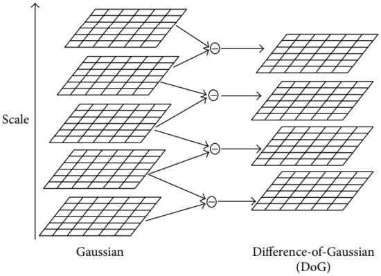
Figure 5.
The left column represent the images resulted from the Gaussian functions with different values of K. The right column displays the Difference-of-Gaussian images that resulted from the subtraction of neighboring images. Adapted from [27].
These DoG images are stacked, and each sample point is examined between its neighbors from the same scale layer and nine neighbors from the scale above and below. Based on the comparison of the sample point with all of its neighbors, it can be viewed as a feature candidate if local maxima or minima, depending on whether the value is larger than all of its neighbors or smaller, respectively, is detected Figure 6.
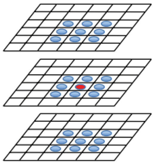
Figure 6.
Detection of feature points. The sample point is marked by a red circle, and its neighbors from the same and different scales are marked with a blue circles. Adapted from [27].
This process is often repeated on an image pyramid or images that have differently scaled in size, so features at different scales are also identified (i.e., features from a closer object still remain even if the object moves further).
The feature candidates are added into a database and a descriptor is computed. A descriptor is a detailed vector of position, scale, and principal curvature ratios of the features candidates neighbors allowing the rejection of candidates with low contrast, due to them being highly sensitive to noise making them bad features or poor location.
An early implementation of keypoints location only stored the information of the sample point’s location and scale [2]. A more stable that also improved feature matching significantly was later developed and applied by interpolating the location of the maximum using a 3D quadratic function [28]. This allowed the application of the Taylor expansion to the center of the origin’s sample of the Difference-of-Gaussian image (Equation (8)).
In order to identify an extremum, the x derivative of the function is performed and zeroed (Equation (9)).
Replacing the Equation (9) into (8) results in the extremum value (Equation (10)), and it is with this function that sample points are rejected if low contrast values emerge.
Therefore, in this way, sample points that present an extremum value of under a certain offset (an offset of 0.03 in image pixel values is used in [3], where pixel values are considered in the range of [0,1]) are considered low contrast and therefore discarded.
Because features in edges stand out when the DoG function is used, alongside the rejection of low contrast keypoints, rejection of inadequately determined keypoints along edges helps improve stability, as these particular features are sensitive to minimal amounts of noise.
Hence, to analyze the suitability of an edge keypoint, a 2 × 2 Hessian matrix is estimated at the position and proportion of the keypoint(Equation (11)).
Alongside the findings in [29] and knowing that the values of the Hessian matrix are proportional to the maximum and minimum normal curvatures of D, direct calculation of derivatives of the matrix are not required as only their ratios are needed. Considering the largest and the smallest values, the determinant and trace of the Hessian matrix can be calculated by the sum and product of them, respectively.
From the result of Equation (13), if the determinant is negative, it means that the curvatures carry opposing signs, and in this case, the keypoint is rejected as it is not an extremum. In case the determinant is positive, the relation between and is calculated by assuming . Substituting this expression into Equation (14), the ratio of the principal curvature can be calculated.
From this, a keypoint is discarded if it presents a ratio above the threshold (15) as it means that the difference between larger and smaller values is substantial, so keypoints presented in these locations will suffer distortion from noise.
Figure 7 illustrates the step mentioned above. Gaussian filters are applied to the image in Figure 7a. DoG images are computed, and keypoints are extracted by identifying sample points that stand out from their neighbors. Figure 7b illustrates the 3601 keypoints detected. An analysis of the keypoints is performed in order to discard those that present low contrast using Taylor expansion. Analyzing Figure 7b,c, it can be noted that most keypoints located in the sky, around the bird and the flower, were rejected due to having low contrast. Figure 7c displays the remaining 438 keypoints after the rejection of those with low contrast. The prevailing keypoints are further examined based on their principal curvatures ratio. Those whose ratios are higher than a certain limit are rejected. As such, when comparing Figure 7c,d, it can be noticed that the density of features on the wings and the chest of the bird have decreased. Figure 7d exhibits the remaining 380 keypoints.
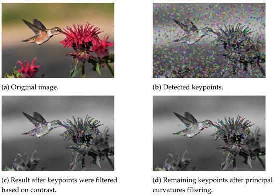
Figure 7.
Detection of keypoints and further selection of invariant features: (a) illustrates the original image; (b) illustrates with circles the keypoints identified by the Difference-of-Gaussian function. These keypoints are then filtered based on their contrast. The remaining keypoints are depicted in (c); (d) represents the prevailing keypoints after further exclusion due to principal curvatures ratio threshold. Adapted from [3].
In the situation where images are flipped or rotated, the keypoint computed in a normal image would not coincide with one of a rotated image mainly due to the algorithm not expecting an image with a different orientation. An early approach to deal with the rotation of the images was to search for keypoints that would remain despise the rotation applied to the image [30]. However, this method restricts the number of keypoints that can be used and could lead to the rejection of valuable keypoints.
In order to obtain invariance in image rotation, Lowe et al. [3] proposed a consistent assignment of orientation, based on the local properties of each feature candidate allowing the descriptor to store information regarding the feature orientation. This is done by taking each image around the same scale magnitude and computing gradient values and orientations using pixel differences. The result would be a histogram composed of gradient orientations of the sample points around the keypoint. A directional peak in a local histogram correlates to a predominant direction in the local gradient. To determine a keypoint direction, the highest peak value alongside all the peaks which have values within 80% of the highest one are used. Furthermore, in locations with several peaks of similar intensity, keypoints will present different orientations but with the same length and location.
Having computed the location, scale, and orientation of each keypoint, a local descriptor can be computed based on these invariant parameters making the descriptor also invariant but also distinctive enough when compared to other descriptors. To do this, an approach from [31] is used. The approach is based on a specific neuron complex in the primary visual cortex, a biological vision model that reacts to gradients at a special orientation. However, the gradient is allowed to shift on the retina over a limited area. This way, it allowed the complex neurons to recognize and matching 3D objects from a series of angles. In this study, experiments using animal and 3D shapes together with changes in position resulted in better classifications under 3D rotation.
In SIFT, the gradient intensities and direction are set around the location of the keypoint from the same Gaussian blur. Orientation invariance is obtained by rotating the gradient orientations and descriptor position relatively to the keypoint direction. To avoid swift and unexpected adjustments in descriptors with small intensities and to give gradients located further from the middle point of the descriptor less weight, a Gaussian weight function is used to attribute levels of importance based on its location sample point ( circle in Figure 8).
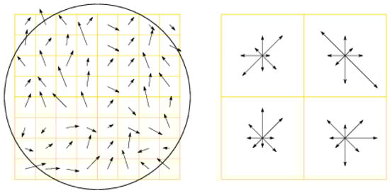
Figure 8.
Keypoint descriptor computation. On the left image, the arrows represent the gradients and direction of neighbors around a keypoint. The circle displays the Gaussian weight function. The right image shows a 4 × 4 sub-region keypoint descriptor resulted from the sum of orientations and intensities from the left histogram. The arrow size reflects the total of gradient from that orientation within the region. Adapted from [32].
On the right of Figure 8, a keypoint descriptor is illustrated. Here, four histograms are displayed, each with eight orientations. Each arrow represents a direction and the size reflects the sum of each arrow of the region. The descriptor is a vector composed of all orientation values of each histogram entry.
At last, the descriptor vector is subjected to adjustments regarded lighting by normalizing it to unit length. Lighting changes that can occur during the image capture, be it camera saturation or illumination changes, can impact the way surfaces reflect light causing orientations to be changed and intensities to be altered. By adjusting the lighting, the effect of large gradient magnitudes is reduced and more priority is put on orientation distribution. Furthermore, if pixel values are a product of constant times itself then the gradient is also a product of the same constant. By normalizing the vector, this product is canceled. If the brightness value is changed by adding a constant to each image pixel, the gradient values will not change as they are computed from the difference of pixel values. This way, the descriptor can be invariant to illumination variation.
Moreover, although Figure 8 represents descriptors as a 2 × 2 vector composed of orientation histograms, experiments from [3] reveal that the preferred results are achieved when a 4 × 4 histogram vector each formed with eight directions. This way, a descriptor vector composed of 128 dimensions is able to provide consistent matching results when compared to lower and higher dimensional descriptors, due to lack of resolution and increase in distortion sensitivity respectively, and also maintain a low computational cost during the matching process.
3.2.3. Feature Matching
From the features extracted from the previous step, the created database of features is used to match similar enough descriptors from different images and pairing images that contain them.
To do this, feature matching algorithms are needed. Csurka et al. method defines features through the use of visual words [33]. The Bag of Words (BOW) algorithm uses the features extracted from the step before and based on the visual representation of the feature is given a unique word used to describe the feature. These words are then used to construct a vocabulary. The feature matching process is done by the comparison between features detected of the new image against the words already present in the vocabulary. In case a word is not present, it is added to the vocabulary [34]. A secondary approach denoted Fast Library for Approximate Nearest Neighbor (FLANN) allows the matching of features by their euclidian distance [35].
In this step, the FLANN process is used, and the algorithm is explained ahead.
This process will create compressed pkl files that store information related to which image has matching descriptors.
In order to match features across images, a descriptor from the database and a keypoint from the image are compared, and it is said to have found a good match when the same values between the descriptors are similar. However, images with similar patterns can create very similar descriptors which can lead to ambiguity and wrongfully matched features. As such, a ratio test is applied to the keypoint. From the database, two descriptors are chosen based on the smallest Euclidean distance they have with the keypoint. The distance between the descriptor with the best match is tested with the keypoint and compared with a threshold. In case the distance is larger than the threshold value, then the descriptor is not considered a good match with the keypoint. Inversely, it is said to be a good match between descriptor and keypoint if below the threshold.
Finally, the match is only accepted if the distance between the best match descriptor and the keypoint is considerably better than the distance between the second-best match descriptor and the keypoint. From the experiment, a distance ratio of 80% allowed the rejection of 90% of false positives whereas less than 5% of correct matches were discarded [3].
Additionally, the exact identification of the closest descriptors in space is only possible through exhaustive search or the use of the k-d tree from Friedman et al. [36]. Nevertheless, due to the high number of points, an exhaustive search would require too much computational cost, and the use of the k-d tree would not provide significant improvement. For that reason, a similar algorithm to the k-d tree is used, named Best-Bin-First (BBF) [37].
In k-d trees, the search method splits the data by their median from a specific attribute or dimension, and the process repeats as long as there are remaining dimensions. This method provides some advantages that allow finding nearest neighbors at a cost of accuracy because there is the probability that the effective nearest neighbor is not on the region that the k-d tree returns. The downside of this method is the computational speed is only better than exhaustive search when 10 or fewer dimensions are used. In SIFTS case, the descriptor has 128 dimensions.
The BFF algorithm uses an adjusted search method to the k-d tree where the closest distance to the keypoint is checked first. This method allows the algorithm to return the closest neighbor with high probability as further searches are not required after a specific number of regions have been checked. This method provided a boost in processing to up to twice the time taken by the nearest neighbor search with only a 5% loss of correct matches. The method also allows the implementation of the distance ratio of 80% between the nearest and second nearest neighbors as stated above.
Occasionally, some objects on images can be partially obstructed by other objects, and this can happen due to movement or from perspective angles. This way, the algorithm must be capable to detect partially blocked objects with just a few features. From the experiments, Lowe et al. found that an object recognition algorithm can detect an object using a minimum of 3 features, and high error tolerance fitting methods like RANSAC would perform poorly due to the percentage of inliers being lower than 50% [3]. From this, a Hough transform is used to cluster features [38,39,40].
The Hough transform interprets the features and clusters them following the object poses present in said features. When multiple feature clusters are interpreted to follow the pose of a previously found object, the chance of the interpretation being correct increases. As each descriptor stores information regarding the location, scale, and orientation, an object position can be predicted using Hough transform Figure 9.
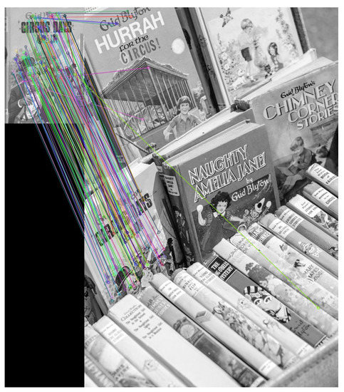
Figure 9.
On the left, an image is given to the algorithm to extract its features. The features detected of the image are then compared with features of the right image. The lines illustrate the corresponding features between the two images. Adapted from [3].
Finally, the object prediction is accepted or rejected based on a probabilistic model from [41]. Here, the estimated false matches of the object are computed based on the model’s size, the volume of features, and model fitting. The presence of an object is given by the probability of Bayesian statistics from the number of paired features.
The object is deemed present if the analysis returned the probability of at least 98%.
3.2.4. Track Creation
Using the files created from the previous steps, feature tracking is computed.
Features identified from each image alongside the file containing the images that matched the features detected are loaded and the images are labeled as a pair.
A feature point track is a collection of image positions containing a specific feature in other images which lets the algorithm know how the feature has developed over the duration of the image capture [42]. This allows the creation of constraints used by the SfM algorithm during the reconstruction.
A tracks.csv file is created at end of this step, containing a unique ID given to the track, a feature ID given to the feature when it was extracted, the coordinates of the feature in an image, and its RGB values [19].
Additionally, based on the GNSS information, the origin of the world reference frame is assumed and stored in reference_lla.json.
3.2.5. Reconstruction
Through the feature tracks created before, the map is constructed using 3D positions and the position of the cameras.
In this step, an incremental reconstruction algorithm is used by first taking an image pair and gradually appending the rest of the images to the reconstruction until all the images were added.
The list of image pairing from the tracking step is loaded and sorted by their reconstructability. This criterion is derived from the displacement that occurs on two images, parallax, similar to human visual perception. To evaluate if a pair of images possess enough displacement, a camera model is attempted to be applied to the two images without any form of transformation besides rotation. The pair is then considered possible starting points if a substantial number of matches between the camera model and the images are exhibited but not explained by the rotation transformation. Outliers are computed, and the image pairs are sorted by the number of outliers.
The image pairing that presents the most reconstructability, and as such the least outliers, is selected as a starting point.
Now an iterative operation is performed to gradually grow the reconstruction. On each iteration, an image is selected based on the number of similar points already present in the reconstruction. The image’s initial pose is estimated, and adjustments are made to the reconstruction to minimize reprojection errors using [43]. The image is appended to the reconstruction, in case the estimation is successful and tracks that might arise from this image are checked. If necessary, a bundle adjustment process is performed to correct camera and 3D points poses as well as minimize the reprojection error of all images in the reconstruction [44,45].
The result of this step is a reconstruction.json file which contains the information regarding the origin of the reconstruction from reference_lla.json, information about the camera used, the images that integrate the reconstruction with the respective rotations, translations, and scaling operations performed on them and the estimated positions and colors of the 3D points in the model.
Furthermore, the sparse model can be exported as a point cloud, illustrated in Figure 10.
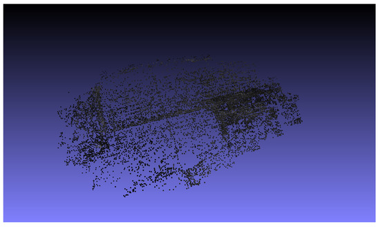
Figure 10.
Sparse point cloud representation of the surveyed area.
3.2.6. Undistort
As it can be observed by the Figure 10, the sparse model exhibits low point density, and large gaps are present between points. Therefore, no substantial information can be used to make an assessment of the surveyed area. Thus a denser model is needed.
In order to generate a denser point cloud, the distortion present in the images integrated into the reconstruction needs to be removed. When 3D scenes are captured by cameras, and they are projected into a 2D plane and depending on the type of camera and/or lens used, this capture can add errors. The error that is intended to be corrected in this step is the radial distortion. This error can be evident in images where straight structures present themselves bent when projected onto images Figure 11.
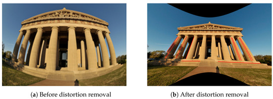
Figure 11.
Illustrations between image before and after distortion removal. The red lines represent straight lines/structures in real world. Adapted from [46].
The undistortion process of the image is done by creating a second image with the same projection type as the camera of the distorted image and the same image size. Then the pixels of the distorted image are remapped to the new coordinates of the undistorted image. In case the pixel’s new coordinates are outside of the range of the image, then interpolation for non-integer is performed.
The Structure from Motion steps performed on the images is illustrated in Figure 12.
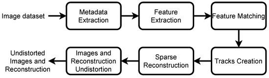
Figure 12.
Sequential diagram representing the applied Structure from Motion steps.
3.3. Multi-View Stereo
Using the undistorted images and the reconstruction, a denser point cloud can be computed. For this, a concept of stereopsis is used where depth is perceived through visual information from two separate viewpoints. As a natural improvement to the two-view stereo algorithms, multi-view stereo (MVS) algorithms were developed which, instead of using only two images with different viewpoints, started to use multiple viewpoint images in between the two original viewpoints to increase stability against noise [47].
From Furukawa et al.’s work, MVS algorithms can be divided into four categories: voxels, polygonal meshes, depth maps, and patches [48].
Voxel-based algorithms use a computed cost function estimated from the object’s bounding box [45]. With this function, [49] scanned the scene to identify unique voxel colors constant over possible interpretations across a discrete 3D space. Reference [50] estimated the least surface size needed to encompass the largest volume possible maintaining photo consistency using graph-cut optimization. Because accuracy of all methods mentioned so far is reliant on the voxel resolution, [51] proposed an algorithm that does not require the surface to be totally inside a visual hull but uses smaller meshes that when stitched together form a volumetric multi-resolution mesh surrounding the object. The downside of the voxel-based algorithm requires that the object presents a degree of compactness, so a bounding box can be tightly fit. As such, the voxel algorithms are only capable of reconstructing small compact objects as the processing and memory costs requirements become extremely high for larger scenes [52].
Polygonal meshes are an improved densification method that relies on the voxel space representation as such, like before, larger scenes require high processing and memory costs. The polygonal mesh algorithm takes a selected starting point and progressively adds further meshes to it. Faugeras et al. [53] defined initial surfaces through partial derivatives equations which then would attach to the object. A different approach took information regarding the texture and shape of the object and combined it into an active contour model. However, this reconstruction was only accurate if the initial surface of the object matched the active contour model [54]. A minimum s-t cut generated an initial mesh that would be processed using a variational approach to register details of the object [55]. This last improvement led to [56] to define the reconstruction to a series of minimal convex functions by establishing the object’s shape as convex constraints reducing the number of possible functions.
A downside to this algorithm is that it depends on the reliability of the initial guess which becomes difficult for larger scenes such as outdoor surveys [48,52].
Depth maps are generated from the views of integrated images in the reconstruction and combined into a space model, often named depth map fusion, based on the visibility rule [45]. This rule states that a single view must only intercept the scene once from the camera pose and the position of the view. Prior works such as of [57] used matching methods on a set of pixels to construct depth maps and combine them. Merrell et al. obtained surfaces using a stereo technique that produced noise, whilst overlapping the depth maps and eventually fusing them based on the visibility rule [58]. Later works such as of Fuhrmann et al. [59] developed a MVS method that produces dense models through depth maps resulted from images of a survey. The depth maps are matched in space, and a hierarchical signed distance field is built. A hierarchical signed distance field is, as explained by the authors, a set of octaves or divisions of the space into scales where images of the same scale are attributed to the same octave. The purpose of the division into octaves is the difficulty of acquiring enough information of a set region due to the presence of depth maps of different scales.
Finally, a patch-based technique develops bits of patches through textured points and spreads them over to other textured points covering the gaps between points. An initial approach was achieved by Lhuillier et al. [60], which resampled points of interest from the sparse reconstruction, this way creating denser point clouds. A second approach was proposed by Goesele et al. [61] in which it reused the features from the SIFT algorithm to build a region growing process which was tested with obstructed object images. With these techniques, Furukawa [48] was able to develop a MVS method, named Patch-based MVS (PMVS) that still is being used today and is considered one of the renowned MVS methods to reconstruct larger scenes accurately and with a high level of model completeness. The PMVS algorithm can be divided into three steps, patch creation, distribution, and filtering. In order to generate a set of patches, a feature extraction and matching process is performed. This set of patches is then distributed over the scene so that each image cell has at least one patch. Each image cell is then filtered three times. The first filter removes non-neighboring patches on cells that present more than one patch. The second filter applies a more strict visibility consistency where the number of images from where the patch can be seen. if this number is lower than a threshold, the patch is considered an outlier and removed. The third and final filter is applied in order to maintain a certain level of homogeneity to the area. The cell and the neighbor patches in all images are analyzed and compared. if the similarities between the patch and its neighboring patches are not equal to a certain degree, then the patch is filtered. This process is then repeated at least 3 times to create a dense reconstruction with the least amount of outliers.
In this work, the densification process of the sparse reconstruction obtained from the process of SfM was done through the open-source library OpenMVS available in [4,62]. This library applies the patch-based algorithm for 3D points inspired from [63] and is introduced ahead. The patch-based algorithm used can be divided into four steps: stereo pair selection, depth map estimation, depth map filter, and depth map fusion.
In order to estimate the dense point cloud, the sparse reconstruction and the undistorted images are introduced as inputs of the algorithm.
3.3.1. Stereo Pair Selection
The selection of image pairs is important to improve stereo matching and the quality of the model as such image pairs are done by assigning a reference image to every image integrated into the sparse model. The reference image should present a similar viewpoint to the image and similar dimensions as the accuracy can be negatively impacted if the reference image’s dimensions are too small, or similarities can be hard to match if it is too large.
This way, OpenMVS applies a similar method of [64] to appoint reference images for each image. A principal viewing angle of the camera is computed for each image. Since the sparse model is generated using SfM, the calibration of the camera poses has been done, and a sparse point cloud and respective visibilities were generated. As such, the angle’s average can be attained between the visible points and each of the camera’s centers. Alongside these angles, the distance between the optical centers of the cameras can be calculated. Using these two parameters, angle and distance, suitable reference images can be obtained. First, the distance median is estimated for images whose visibility angle is between 5 and 60. Second, the images whose optical center distance is above twice the median or less than 0.005 the median are filtered. In case the remaining images are below a certain threshold, they are stored as being possible reference images. On the other hand, if the number of remaining images is above a threshold, then the product of the viewing angle and the optical center distance is computed and sorted from lowest to highest. The first threshold images are selected to form the neighboring images. From the neighboring images, the product is of angle and distance is calculate and the one that presents the lowest value is selected as the reference image to form a pair [52].
3.3.2. Depth Map Estimation
The depth map is computed for each pairing, and to do this, a local tangent plane to the scene surface is computed. This plane, denoted by the support plane, represents a plane in space and its normal in relation to the camera’s coordinate system [65,66,67,68].
Given the intrinsic parameters, rotation matrix, and the coordinates of the camera center, each pixel of the input image is associated with a random plane in space that intercepts the raycast of the pixel. A random depth value from a depth range is extracted, and the plane is estimated using the center of the camera’s coordinates. Assuming that a patch only remains visible when the viewing angle is between a certain threshold, the spherical coordinates of the camera’s center can be estimated. Despite the given randomness of the process above, results show that the probability of at least a good prediction for each plane that composes the scene of the image is encouraging, particularly in images with high resolution as the pixel density is higher, in turn, more predictions in contrast to lower resolution images. Moreover, the estimated depth map of the image can be further improved using the computed depth map of its reference image by warping the composing pixels of the image depth map as initial estimates when computing the depth map of the reference image. This way, when estimating the random plane in space of each of the reference image pixels, the estimated plane for a pixel in the image depth map can be used as an initial prediction for the correspondent pixel in the reference image improving the stereo consistency between the image pairing [52].
Having assigned a plane to each pixel of the input image, a refinement process to each of the planes is performed. The process follows a sequence where the first iteration starts from the top left corner and advances row by row until the bottom right corner is reached. The second iteration takes the inverse route, going from the bottom right corner to the top left corner also row by row. The sequence repeats if more iterations are required.
On each iteration, two actions are performed on each pixel, spatial propagation and random assignment.
The former action compares and propagates the neighboring pixels planes of the current pixel. This is done by comparing the combined matching cost of the neighboring pixels with the matching cost of the pixel itself. If this condition is verified, then the pixel’s plane is replaced by the plane of the pixel’s neighbors. This action takes into account the fact of the similarity in planes between the pixel and its neighboring pixels [52,65].
The second action further improves the pixel’s plane matching cost through random assignment by testing parameters of the plane. To do this, a new plane is computed based on the selection of a random plane parameter, and the combined matching cost is compared to the current matching cost of the current plane. If the cost is lower than the current one, then the plane is replaced by the new estimated plane. The range of parameters is reduced by half, and the process is repeated 6 times [52,65].
3.3.3. Depth Maps Filtering
After the depth map estimation of the images, these need to be filtered as the estimation may have produced depth errors. This way, depth maps would match each other, and inconsistencies would occur if the combination of depth maps were performed.
In order to filter each depth map, each pixel from the input image is back-projected into a three-dimension space using its depth and camera parameters. The neighboring images from the stereo pairing are projected intersecting the same pixel on the same point. The depth map is classified as stable if the depth value of the projected point in the camera displays enough similarities with the depth value of the projected point in regard to the camera for at least two neighboring images. Contrarily, the projection is considered inconsistent, and therefore, the depth map is removed [52].
3.3.4. Depth Map Fusion
The final step of the MVS is to merge the depth maps that were estimated and filtered. A simple way of doing this step would be to start with a single depth map and successively add the neighboring depth maps, building a complete depth map, until all the depth maps were added. However, redundancies can occur especially in neighboring images which can lead to miss alignment of images, object’s scale variation, or replicas [58,69].
In order to remove the replicas, a neighboring depth map test is performed. Figure 13 illustrates the test. Each pixel of a camera’s depth map is projected into a 3D space alongside the neighboring camera’s representation of the same pixel. The depth value of the point and each camera projection is calculated and compared with the value of the depth map camera. If the depth value of the neighboring cameras is larger than that of the depth map camera, then the points projected by the neighboring cameras are considered to be occluded and therefore removed from the depth map of the neighbors. In the situation where the projection values are very similar, we consider that the projection of the neighbor camera is a projection of the point from the depth map, so it can be removed from the neighboring depth map. In the final scenario, the projection point is kept if the depth value of the projection camera is smaller than the projected point of the depth map.
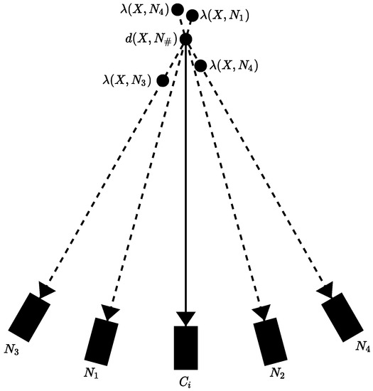
Figure 13.
Neighboring depth map test to remove redundancy. represents the camera of the depth map, and represents the neighboring cameras. The value illustrates the depth value of the projected pixel. represent the depth value of the pixel projected by the neighboring cameras. The depth values of the camera and present depth values larger than the depth value of , and as such, the projected points from and are considered occluded points and removed from the depth map. The point projected by depth value is close to the depth value of , so to avoid redundancy, the point from is removed as the projection of it can be classified as the point projected by . Finally, the point presents a lower depth value than , so its depth map is retained as it does not satisfy either of the conditions stated above. Adapted from [52].
This process is repeated for each pixel of a depth map for all depth maps and finally merged into a single point cloud resulting in a dense point cloud represented in Figure 14a and stored in scene_dense.mvs. As it can be viewed, the reconstruction presents a higher point density and consequently fewer gaps.
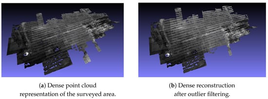
Figure 14.
Dense reconstruction resulted from the MVS algorithm. Figure 14b represents the model after point filtering was applied.
Additionally, noise is removed by applying a statistical filter to the point cloud using [70]. The filtering is done through two steps: an estimation of the average values of each point and its nearest k neighbors and outlier identification by comparing the estimated values with a threshold. In case the estimated value is above the threshold, it is marked as an outlier. The removal of these is done by a range filter which runs by each point and removes the ones that are marked as outliers from the data following the LAS specification [70]. The result of the filtered point cloud is presented in Figure 14b.
Figure 15 illustrates the results obtained by applying the described processes to the input.

Figure 15.
Diagram representing the applied Multi View Stereopis steps.
3.4. Meshing Reconstruction
From the work of Khatamian et al. in [71], the surface reconstructed can be organized into two categories: explicit and implicit surfaces.
Digne et al. define explicit surfaces as representations of a real object in which all the points are present in the point cloud [72]. Furthermore, explicit surfaces can be parametric or triangulated.
In parametric surface reconstruction, B-Spline, NURBS, plane, spheres, and ellipsoids are some of the primitive models used to enclose a random set of points to represent surfaces. However, complex surfaces can be hard to represent using this method as a single primitive model as it might not encompass all of the points and might require multiple primitives to represent the object [71].
DeCarlo et al. [73] developed a parametric surface reconstruction technique where it uses deformations and blending of shapes such as cylinders and spheres. Further development in this type of surface reconstruction involved the application of deformation to the parametric surfaces [74,75,76,77,78,79,80,81,82,83].
The latter surface representation uses a more intuitive technique [71]. Triangulated reconstructions represent surfaces by connecting neighbor points using tethers forming triangles [84].
One of the earliest and whose name is still used when triangulation surface reconstruction is mentioned is the Delauney triangulation [85] where all the points are vertices of triangles, and no point is occluded by any triangle. Amenta et al. proposed the Crust algorithm where it applied the Delauney triangulation to 3D space models by extending the two-dimensional algorithm to 3D space [86] and being able to use unstructured points to generate smooth surfaces. A further improvement of the algorithm was made which addressed the reconstruction of artifacts when a region does not present enough points [87]. In 1999, Bernardini et al. suggested a different method of triangulating surfaces using the Ball Pivoting Algorithm (BPA) [88]. This technique employs different radii spheres which will roll from a determined point to the opposing edge and repeated until all the edges have been encountered. The surface is constructed when three points of the model are in direct contact with the sphere, forming a triangle. This way, points are not occluded as every point will be in contact with the sphere at some point in time, and other points that are in contact at the same time are used to form a surface. Additionally, the use of different radii spheres allows the algorithm to perform even in situations where the distribution of point density is not uniform. Gopi et al. in [89] proposed a surface incremental algorithm where the normal of the points are computed, neighboring points are selected as potential candidate points to be used for surface triangulation, the candidates are filtered using local Delaunay neighbor computation, and finally, the surface is generated from the point and the selected candidate points. Moreover, a faster and memory-efficient incremental algorithm was proposed by Gopi et al. in [90] where a random start point of the surface reconstruction was selected, and the neighboring points were used as vertices to construct vertices alongside the start point. The expansion of the surface was done in a breadth-first-like search.
The second type of surface reconstruction uses mathematical basis functions to estimate the object’s surface based on the input data [71,72]. As such, this method exhibits certain difficulties when representing edges or corners due to the sharp changes not making it suitable for complex surface reconstructions. Nevertheless, improvement in this side of the implicit surface methods allowed this weakness to be addressed using a variational implicit method by including different types of basis functions. In Dinh et al. [91], the inclusion of anisotropic functions into the surface reconstruction allowed the method to retain sharp edges and corners presented in the model. To do this, Dinh et al. performed a Principal Component Analysis (PCA) in a local region of the object. An estimation of the surface is carried out using mathematical functions. Later, Huang et al. improved on this algorithm in [92]. A locally weighted optimal projection was used to reduce the noise present in the data set, removing outliers and uniformly distributing the points. After this operation, the stages presented previously by Dinh et al. were executed. A different approach was taken under Alexa et al. in [93] where the estimation of a surface is done with the assist of the Moving Least Square mechanism (MLS). This algorithm allowed the parallel computation due to the processing being done by regions. Additionally, it allowed downsampling of the surface estimated in order to reduce its output size or to remove outliers, as well as to perform surface upsampling to fill gaps in the surface model. Furthermore, improvements to the MLS mechanism by Oztireli et al. in [94] allowed to fix the noise-induced artifacts and the loss of resolution.
A typical implicit surface method is introduced in [71,95]. Here, the complication of surface estimation is transformed into a Poisson problem improving its noise sensitivity. Later works [96,97] were based on the previous algorithm, and improvements were added to the base algorithm. Contrary to other implicit methods, which rely on model segmentation to develop surfaces and later the usage of methods to combine the multiple segmented surfaces into a single one, Poisson considers all the models when computing the surface without relying on model segmentation and further merging. This way, it allows the Poisson method to recreate smooth surfaces while tackling noisy data through approximation [95].
In this work, the meshing process is done using the open-source library made available by Kazhdan et al. in [4,98]. This library applies the Poisson surface reconstruction algorithm inspired from [95] to which the steps are explained ahead and illustrated in Figure 16. The algorithm can be divided into steps: definition and selection of function space, vector definition, Poisson equation solution, and isosurface extraction.

Figure 16.
Diagram of the workflow to generate mesh model.
3.4.1. Space Function
An adaptive octree is used in order to represent the implicit function, as the accuracy of the representation is higher the closer the implicit function is to the reconstructed surface, and to solve the Poisson equation. Additionally, in order for the algorithm to run efficiently, conditions must be satisfied. The vector field needs to be represented, with a certain level of precision and efficiency, as a linear sum of functions of each node o from the octree, . The Poisson equation represented by a matrix of functions needs to be solved efficiently. The indicator function representing the sum of functions needs to be quickly and precisely evaluated [95].
In order to define a space function, a minimal octree is estimated where every sample point is placed in a leaf node of a tree with a certain depth. A collection of space functions are then delineated as
where and represent the center and size of a node o, respectively [95].
A base space function is selected based on how accurately and efficiently a vector field can be represented as a linear sum of the functions . Additionally, by considering each node as its center only, the vector field can be expressed more efficiently as
where D represents the depth of the node and smoothing filter, respectively [95].
By doing this, each sample only contributes once to the coefficient of its leaf node function. Errors that might occur are limited by the sampling width of . Moreover, an unit-variance Gaussian approximation results in sparse Divergence and Laplacian operators as well as the evaluation of the linear sum of in any point q, requires only the sum of the neighboring nodes that are close to q. From this, the base function F can be expressed as a box filter convolution:
as n represents the convolution level [95].
3.4.2. Vector Definition
To increase precision, a trilinear interpolation is used to distribute the point over the nearest eight nodes. This way, an indicator gradient field function can be approximated by:
where s represents a sample point of a sample collection S, represent the eight neighboring nodes with depth D of s, the trilinear interpolation weights, and the sample’s normal directed to the center and assumed to be near the surface of the model [95].
Taking into consideration the uniform distribution of the samples, consequently, a stable patch area, the vector field , can be considered a good gradient approximation of the indicator function [95].
3.4.3. Poisson Equation Solution
Having arrived at a solution for the field vector , the next step is to determine the indicator function of the model. However, is in most cases not integrable so an exact solution might not be reached. In order to resolve this issue, a divergent operator forming a Poisson equation is applied, such as
Additionally, although both and are in the same space, the operators of the Poisson equation, and , may not be. This way, the function is solved by projecting onto a space that is closest to the projection of . However, the direct computation can be expensive and lengthy as the space functions do not originate orthonormal solutions. As such, a simplification of the Equation (19) can be made:
This allows the solution of the function to be the closest possible to by projecting the Laplacian of onto each of the .
Furthermore, to put this into matrix form, a matrix L is defined so that solves the Laplacian inner product for each of the as x corresponds to the entry (o,o′) of the matrix entry L:
As such, can be solved by:
3.4.4. Isosurface Extraction
The final step of the algorithm extracts an isosurface based on an isovalue computed from an indicator function.
In order to find the surface that best fits the positions of the input data, an evaluation of the is performed at the sample points. An isosurface is then obtained by averaging the values of the function.
The isosurface was extracted from the indicator function using an adapted version of the Marching Cubes method [99]. The modifications were vised to subdivide the node if several zero-crossings were associated with it and to avoid gaps between faces isocurves segments were projected from weaker nodes into finer ones.
Nevertheless, inconsistencies can occur due to the presence of noise and outliers on the data as well as uneven point density distribution. To correct this issue, an average value of the function is subtracted to the sample points in order to adapt the function [95]. However, errors can affect the average value so inconsistencies can still occur if a global average value is used. As an alternative, an explicit interpolation of points was added.
To do this, a discretization of the function (19) is performed using Galerkin formula [100]. As a form to produce higher-resolution details on the neighboring regions of the surface while reducing the size of the system, the linear system is discretized by placing the sample points into octree nodes and later correlated with a B-Spline function, for each node [101].
Additionally, a complete grid does not form on any selected octree node and corresponding B-Spline function at each depth as the solution of a given depth cannot be expanded into its successor as the result of the B-Spline function associated with the current node being a sum of functions associated with its successor nodes as well as the successor nodes of its neighbors. This way, the constraints of current nodes are used to adjust its predecessor [101].
Moreover, linear system solvers are important for image processing as these transform linear equations into discrete ones and are often employed in very specific scenarios like image stitching where its solutions are evaluated near the connections of two images. With this in mind, an adaptive, efficient solver was developed in [102] to help solve random levels of a number of finite elements, in symmetric systems, which allows random dimensions and is able to support integral and pointwise constraints.
In order to do this, the B-Spline function corresponding to each octree node is expanded to support B-Splines of any degree. This enables to tweak the system for more sparsity or smoothness, respectively to lower or higher degree of the function. Furthermore, the inner products of gradients that express the coefficients of a Poisson equation are expanded to support a set of partial derivatives and the integration of both bilinear combinations of space derivatives. The dimensionality is allowed by integration and evaluation is separated and performed over the existing dimensions using dimensional windows, neighbor lookups, and template specialization. The constraints are supported by allowing the user to impose the coefficients of functions in relation to the B-Spline levels [102].
Later Kazhdan et al. improved the algorithm presented in [101] as to reconstruct a surface S that would fit the point cloud while also being contained inside a second surrounding surface [103]. This is implemented using the Dirichlet constraint by defining that the indicator field vanishes when outside the surface and only defining space functions that are contained inside of .
However, two issues need to be addressed [103]. One of these issues is the discretization of finite elements [103] so that the exterior nodes are not considered in the basis functions. The method applied by Kazhdan et al. uses a similar approach of [104] where the basis functions can be altered so that they no longer consider the exterior nodes. To accomplish this, the basis functions of exterior nodes are removed, and applying the Laplacian stencil, a linear system can be defined at finer depths. On earlier depths, the basis functions are a combination of finer basis functions that are considered not to be exterior nodes [103].
The second issue that needs to be addressed is the location of leaf nodes that are outside of the surface that needs to be identified. This can be estimated by rasterizing the into the octree and verifying if the depth of such nodes is higher than a threshold, cutting the tethers to the neighboring nodes and separating the triangle into a vector if so.
The nodes that contain the triangle fragments are iterated using a ray-tracing method to identify the center of each face and classifying each face as either interior or exterior of the surface and added into a queue if the label exterior was attributed. The exterior surfaces are then extracted from the overall surface, and the neighbors of such surfaces are tested if they possess more fragments and if the neighbors are classified as exterior surfaces. This process is repeated until no more exterior surfaces are contained in the queue [103]. Finally, the designated exterior surfaces are eroded so that the field vector of earlier levels do not get extracted due to the correspondent B-Splines having larger support.
As a side note, the algorithm is capable of producing two types of models, one incorporating the information of height into the model, the 3D model, and one which employs less influence in this parameter, the 2.5D model. Figure 17a,b represents the 3D mesh model and 2.5D model, respectively. As it can be seen, the 3D model displays more characteristics on vertical objects, where the top is represented as well as the support of it can be delineated. In contrast, the 2.5D model only depicts the top of vertical objects as information regarding the supports of vertical objects is not interpreted [105]. Furthermore, objects in the 2.5D model present a rounder feature when compared to the 3D model. A close of a region where a vertical object is situated is illustrated in Figure 18.
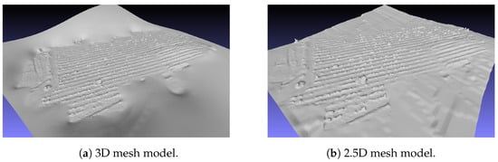
Figure 17.
Reconstructed models of the surveyed area.
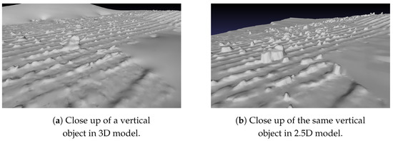
Figure 18.
Objects portrayed in the 3D model exhibit sharper edges as well as the support of vertical objects are better delineated. In contrast, 2.5D model edges are rounder and vertical objects overhung areas do not present any details.
3.5. Texturing Reconstruction
A characteristic of the mesh models is that a single neutral color, often white or gray, is attributed to the mesh surface. However, the information regarding the texture characteristics contained in the dataset is important to analyze the environment of the surveyed site and, in situations where previous surveys were done, to compare and judge the evolution of texture characteristics over time.
In this step, the texture reconstruction is performed using the image set and applied to the mesh model obtained from the step before.
From literature [106,107], the texturing process can be divided into three methods: blending, parameterizing, and projecting.
A common method for texture reconstruction is the blending-based method where images are projected on the surface of the model following its intrinsic and extrinsic camera parameters and in the end mixing all the images into a final texture [108,109,110,111,112]. The downsides of this method are the high noise sensitivity, the appearance of blurring and ghosting in situations where camera poses are inaccurate which can be due to distortion or geometric errors in in-depth map computation, or accumulation of residual camera pose leading to camera shift when computing the trajectory of the camera. Additionally, the method requires the model to be segmented, so the size of the model can affect texture reconstruction [106,107].
The second method segments the mesh surface and places image textures into each segment. The surface is segmented using criteria such as similar area size, angle preservation between directions in the same region, and segmentation that allows the least deformation of each surface [113,114,115,116]. For each segmented surface, a textured image is projected [117] and different deformations applied [118], so it fits best onto the surface. However, as the image suffers deformations, it can lead to inconsistencies. Furthermore, as the partitioning of the mesh, it can lead to artifacts similar to blending methods. Similar to the previous method, the quality of the resulting textured model can be affected by inaccuracies from the camera pose estimation. Bi et al. tried to address this issue using a patch-based method to produce textured images correcting the camera shift [112].
Projection-based techniques assign a single image to one triangle mesh its adjacent triangles forming a texture chart [106,107]. As an algorithm that needs to search all the images when one needs to be selected for a triangle surface is inefficient, Lempitsky et al. proposed a solution that used a Markov Random Field (MRF) energy function to return the best fitting image for each surface [119]. From this work, additional elements were added to improve the selection of images [107,120,121,122,123]. Multiband merging [124] and Poisson editing [125] were implemented as a way to address the issue of visual discrepancies between neighboring surface textures. The projection-based texture reconstruction techniques have the benefit of blurring and ghosting not manifesting as much on the reconstruction when compared to the two other methods [106,107]. However, as the algorithm is run on triangle segments of the mesh, the computation time can be high [106,107].
The method adopted in this work is of a projection-based technique developed by Waechter et al. in [126] and was based on algorithms similar to [119]. The algorithm is made available by Waechter et al. in [4,127]. The algorithm is composed of the three main steps of preprocessing, selection of views, and adjustment of color. The explanation is described ahead.
3.5.1. Preprocessing
The first step in texture reconstruction is to determine the image visibility of the input images. Here, a back face followed by view frustum culling is performed prior to analyzing the surfaces for any occlusion that might exist. To check for occlusion, the intersection between the mesh model and the raycast between the camera and the surface is calculated [128]. By doing this, the rendering process is more accurate without being too affected performance-wise [109].
3.5.2. View Selection
After the computation of image visibility, a label l is computed using the Markov Random Field energy formula (Equation (25)) and assigned to a surface mesh . The label informs which image view is going to be used to texture that specific surface.
where returns how good the view fits the surface, and indicates the visibility of discrepancies between the textured edges of adjacent surfaces.
For the first term, the Gal et al. [120] function was used, where the data term is calculated based on the image’s gradient value that is projected into the surface with a Sobel operator and the pixels within the surface’s projection of the gradient image are summed (Equation (26)).
This method is preferred as it recognizes out-of-focus blur where surfaces closer to the camera exhibit larger projection areas but may not be in focus, therefore leading to texture blur [126]. However, this method does not reject views where obstructing objects were captured in the images but not reconstructed as often the obstructing objects present larger gradient values than its background [126]. To provide texture cohesion, an additional step was implemented in order to maintain photo consistency.
To maintain texture consistency, the projected surface mean color is calculated for each view, and all the views that view the face are marked as inliers. The mean and covariance matrix of the mean color inliers are computed, and using a multivariable Gaussian function each view is analyzed. The Gaussian function values of views that are above a determined threshold are stored. The last three steps are repeated until either the entries of the covariance matrix are lower than , the inversion of the covariance matrix becomes unstable, the number of inliers drops below 4 views, or 10 iterations were completed [126]. This method is an adapted version of the works from [129,130] where the assumption is made that most often views will see the same color except in situations where obstructions occur. By calculating the mean or median, the views with inconsistent colors can be rejected.
3.5.3. Color Adjustment
The last step of the algorithm relates to the color correction of the texture patches. An issue that was reported from the Lempitsky et al. method was the color correction was only implemented on a single location, the vertex point between the edges of two adjacent images. This is considered an issue, as image texture might not correspond to the object texture due to inconsistencies of camera pose. Waechter et al. used the edges of adjacent images to perform the adjustment [126]. The process is illustrated in Figure 19.
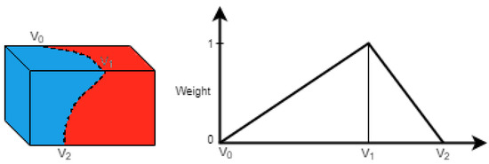
Figure 19.
Color adjustment method. The left image illustrates a mesh. The right image represents the variation in sample weight in relation to the distance to . Adapted from [126].
From the figure, it can be concluded that the point is located on the edge between the red (R) and blue (B) patches. The average sample color from the red image, , between the segments and is calculated based on the linear weight transition of the right image of the Figure 19, where sample color further away from has less influence over the average value while has a color weight of 1. The same method is applied to calculate the average color of in the blue image, . Then, both values are inserted into Equation (28)
where g is an additive correction value computed for each vertex. The first term assures the similarity between the color on the left and on the right is as close as possible while the second term aims to reduce the differences between adjacent vertices inside the same texture region. Additionally, the correction of the color of only the luminance channel is insufficient Therefore, the color optimization is performed on the three channels in parallel [126].
Furthermore, the discrepancies are not all removed by color adjustment, so a second adjustment is performed using local Poisson image editing [125]. A 20-pixel wide patch is selected to perform the Poisson editing. The outer blue and outer red borders are used as boundary limits of the Poisson equation (Figure 20). For each pixel on the outer region, its value is the mean value of the pixels of the image to which the patch is correspondent. For the pixels on the inner region, the correspondent pixel color of the image is assigned to it. All the patches are solved through parallel linear systems using Eigen’s SparseLU factorization [131]. Each patch is only factorized once as the resulted matrix remains unaltered for all color channels. Moreover, as this method does not involve the mix of two Laplacian image matrices, no blending is involved [126].
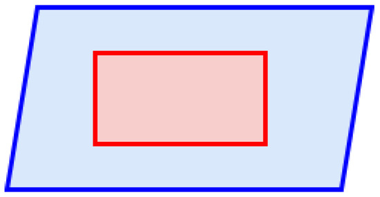
Figure 20.
A 20 pixel wide patch used in Poisson editing. The outer blue boundary, in dark blue, and outer red boundary, in dark red, are used as boundary limits of the Poisson equation. The value of the pixels on the blue patch are assigned by computing the mean pixel values of the image that corresponds to the patch. Pixels on the red patch are given the same value as of the correspondent pixel in the image. Adapted from [126].
A visual representation of the steps taken to generate texture models is illustrated in Figure 21.
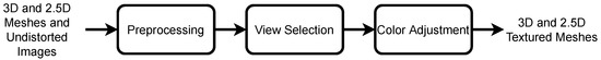
Figure 21.
Flowchart illustrating the steps taken to compute texture models.
3.6. Georeferencing
The current step of the workflow will attach the geolocation of the resulting model from the previous step into the real-world reference. For this, computed coordinate files such as coords.txt were computed at the start of the workflow when the images were being prepared to be inserted into the SfM workflow and contained the coordinates extracted from each of the images, and geocoords_transformation.txt file resulted during the SfM reconstruction where the model is built based on the relative position of the images and later aligned with the GNSS information available. In situations where these files are not present, the extracted EXIF information of the images can be used to georeference the reconstruction. On the other hand, the algorithm will favor the geocoords_transformation.txt if both files are present.
To georeference the model, information from the coordinate files is extracted and converted, if need be, to a certain format, and a transform matrix is built. The textured model is loaded and its mesh is extracted. The transform is applied to the mesh and each surface texture is iterated once and applied specific transformations using Geospatial Data Abstraction Library (GDAL) [132].
Additionally, the point cloud obtained in the filtering step can also be georeferenced by applying the transformation to the point cloud using a Point Data Abstraction Library (PDAL) [70].
It should be also of note that the georeferencing process is performed first on the 2.5D model and subsequently on the 3D mesh. This is done so that the transform matrix used on the 2.5D model can be later used for the 3D mesh. If the process was inverted, elevation models and orthophotos might not align [4]. Figure 22 represents a diagram of the georeferencing process.
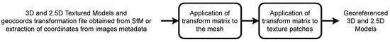
Figure 22.
Georeferencing workflow.
3.7. Orthomap
The last step of the workflow involves generating an orthomap of the model. An orthomap aims to display a general map of the surveyed area by correcting the geometry of photos, so a scale homogeneity is present. A correction of perspective is also performed over the captured images in order to give a perception that the images were captured and the camera was in parallel planes [133]. This way, a true distance between points can be measured [134].
In this step, the georeferenced model from the previous step is loaded. The mesh and the textures are extracted, and a boundary of the reconstruction is established. This boundary model consists of all the vertices that belong to the reconstruction. From the boundary model, a transform matrix is extracted and applied to the mesh using a pixel by pixel method so that the mesh can be encased into the area of an orthophoto. Following this pixel-by-pixel transformation of the mesh, textures are applied back to the mesh surface using a dictionary that mapped the ID of the surfaces with the ID of each texture patch.
The orthomap is then converted into a GeoTIFF type of file. The reason GeoTIFF type was used is that it allows the information regarding the georeferencing to be stored inside a TIFF file [135]. The conversion is done by a rasterization process using GDAL library [132]. The reason for using this library is that allows the georeferenced coordinates of the model to be preserved during the rasterization process.
Next, a cutline file is generated in order to express the zones of which should be removed, and the regions are cropped using a tool named gdalwarp of the GDAL library [132]. Additionally, sharp edges of the reconstructed orthomap are smoothed using a feathering technique [4].
The result of the orthomapping process can be seen in Figure 23.
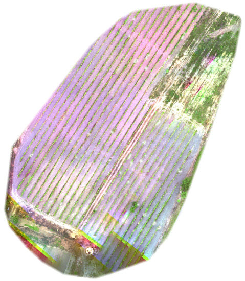
Figure 23.
The resulting orthomap of the surveyed area with approximately 0.2 m between two consecutive points of the point cloud.
Figure 24 represents the steps taken on the orthomapping process.

Figure 24.
Ortho map flowchart.
4. Experimental Results
This section aims to display the results obtained from the implementation of the workflow.
The model was implemented in Python programming language with integration of the aforementioned open-source algorithms. The maps were generated using a i7-8700@3.20 GHz processor computer with 64 Gb of RAM running a 64-bit Ubuntu 18.04 LTS distribution.
It should be noted that due to the high computational power required to process the data sets, an i7-8700@3.20 GHz processor computer was used, as a lower processor (i7-7700HQ@2.80 GHz) resulted in memory issues.
The implemented workflow was tested using data sets that were obtained using UAS. Here, the camera used was calibrated before the surveying flight and the distortion present in the images were removed. The workflow was tested on three different types of data sets. The first data set tested used the most common type of images, RGB images, as they can be collected using most cameras. This test aimed to evaluate the ability to generate models using images that could be captured using mundane devices such as smartphones.
The following data set used was the multispectral images. Here, a MicaSense RedEdge-M camera was resorted to as it allowed the capture of images on five different bands: three bands of the visible spectrum (blue, green, and red) and two bands from the invisible band of the electromagnetic spectrum, red-edge and near-infrared. Due to the design of the camera’s lenses, an image calibration process is required to correct any displacement that occurs. Additionally, image sets of a single band were also used to test digital model reconstructability.
Finally, the last data set tested used thermal images captured using a Flir Vue Pro R camera. Because of the difficulty in feature detection and as a result of matching, an adaptation was implemented.
The Table 4, located at the end of the paper, shows some characteristics obtained from each data set.
Table 4.
Characteristics of data sets and their produced models.
4.1. RGB Product
One approach taken with the program was the reconstruction of a digital model based on RGB data. This data can be obtained by any portable camera with varying degrees of resolution.
The RGB data set is composed of 353 images taken at approximately 280 m high. The altitude and velocity of the UAV enable an image to be taken approximately every 2 m, thus allowing high region overlapping which are important for the SfM workflow. Each image captured is stored, and information regarding the GNSS coordinates and the band name, in this case RGB, are stored in the metadata of the image.
A digital ortho map and 3D model reconstruction are generated by applying the workflow to the image set (Figure 25 and Figure 26).
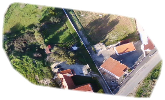
Figure 25.
Orthomap generated from RGB imagery. Two points of the point cloud are approximately distanced by 0.09 m.
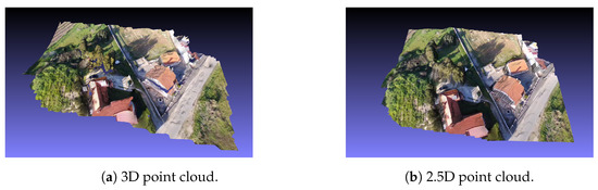
Figure 26.
Point cloud models obtained from RGB images.
4.2. Multispectral Product
A second approach taken was the reconstruction of models based on multispectral imagery [136].
In this approach, a MicaSense RedEdge-M camera is used. This camera allows the capture of images on five distinct spectral bands, three on the visible spectrum, red, green, blue, and two on the invisible spectrum, near-infrared, and RedEdge. The captured image’s metadata contains the GNSS information relayed from a Global Navigation Satellite System device to be used to georeference the model and a Downwelling Light Sensor (DLS) which will measure the ambient light during flight. The latter information is relevant to correct the brightness variation that can occur due to sunlight obstruction by clouds or any other objects during the image capture.
Furthermore, the reconstruction process presents slight divergences when a single band or multiple bands are used to reconstruct a multispectral model.
In order for the program to detect if multiple bands are present, an analysis of the metadata is performed. If multiple band names are discovered during the analysis, the algorithm is altered, so images from multiple bands are integrated into the reconstruction.
The notable differences are explained ahead.
As for a reconstruction of a single band, the blue band was chosen as the band to generate a single band model. The data set used is composed of 36 images corresponding to the blue band taken at approximately 270 m high. Based on the GNSS coordinate displacement and the image file name, it is deduced that an image was captured once every 43 m leading to a region overlapping of roughly 50%. As the band name always refers to the blue band on the metadata extracted from the image set, the program proceeds identically to the workflow taken on an RGB model.
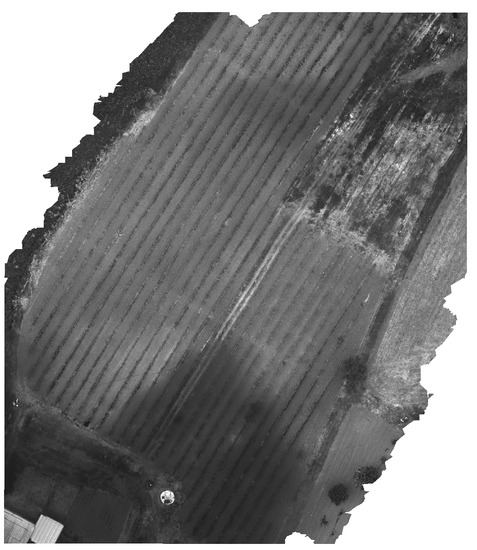
Figure 27.
Orthomap generated from single band, in this case the blue band, obtained from MicaSense camera. Two consecutive points are distanced approximately 0.2 m apart from each other.
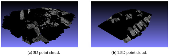
Figure 28.
Point cloud models obtained from the processing of images from a single band, in this case the blue band.
Multi Band
When multiple band names are detected on the image set, the algorithm takes the smallest band index images of the data set. From the study of the MicaSense camera documentation, the band indexes are sorted by blue, green, red, near-infrared, and red edge, from smallest to largest respectively.
The initial process of the SfM workflow, namely, metadata extraction, feature detection, feature matching, tracks creation, and finally sparse reconstruction, are performed on the blue band (primary band), the lowest index band of the data set.
From this point on, the main workflow suffers a slight deviation compared to the standard procedure.
As the reconstruction file contains the images that are integrated into it, images from the other bands (secondary bands) are matched against the images of the primary band. Alignment matrices are computed provided the secondary band images present good matches with images of the primary band. The alignment matrices are a product of homography.
Homography is described as a method to transform the perspective of a plane into another perspective, or in other words, is the reprojection of plane from one camera viewpoint into a different viewpoint. In order to accomplish this, homography uses SIFT to detect features between images. To match the features, two techniques are used. A Brute Force matcher is ran first by using the created feature descriptors of one image and matching with the features of the second image based on distance criteria, returning the closest one. The benefit of this method is that its processing time is rather short as only a few features are compared due to the distance criteria. However, a different approach is required, in case no results are returned from the Brute Force matcher.
The second approach to matching features uses Enhanced Correlation Coefficient (ECC) developed by Evangelidis et al. [137].
Image alignment algorithms can be characterized by the estimation of a suitable geometric parametric transformation that correctly maps the coordinates systems of both images and the suitability of the parameters of said transformation. The mapping of coordinate systems between two images can be done based on the discrepancies between two complete image profiles, pixel-based or, for specific features, feature-based [137]. To evaluate the suitability of parameters, two approaches are defined. A gradient-based approach, often used in computer vision applications, is adopted due to its low computation cost requirement. However, the convergence can fail when homogeneous areas are present. The second method, the direct search technique, although not suffering from the convergence on homogeneous regions, has higher computational requirements than the gradient-based techniques.
From this, Evangelidis et al. proposed a gradient-based image algorithm, Enhanced Correlation Coefficient (ECC), as a new method to compute image alignments [137]. As a gradient-based algorithm, ECC is capable of achieving high accuracy in parameter estimation. Additionally, as the correlation coefficient between two images is taken as an objective function, its performance is invariant to illumination changes in images. Therefore, the benefits of the ECC are the low computational cost and the invariability to contrast and brightness of photometric distortions. The ECC calculates the alignment of two images by estimating the 2D geometric transformation, characterized as a motion model of a reference image. This model is stored in a warp_matrix that is applied to the input image, resulting in a warped image registered in the coordinate system of the reference image.
Following the homography of images, the distortion present in the images is removed by using the distortion values present in the metadata of the image to calculate the undistorted values of each pixel and remapping them to a new image.
At the end of this, similarly to a single band reconstruction, an N-View Match file format is created for each band composed by the integrated images of the said band in the reconstruction, its normalized focal length, the transform matrix, and pose of each band in relation to the origin of the model.
From this point on, the steps are run similarly to a single band reconstruction with small deviations in the texturing and georeferencing steps.
On the texturing step, the textured 3D model is built similarly to a single band, based on the primary band. However, separate textured 2.5D models are generated for each band present.
Accordingly, the georeferencing step is performed over the created models using geocoords_transformation.txt created on the SfM step.
In order to generate a multispectral model, the images taken from the MicaSense camera were introduced as the dataset into the program. This dataset is composed of 180 images divided into the 5 captured bands, red, green, blue, near-infrared, and red edge. Similar to the single-band experiment, the images were taken at an altitude of roughly 270 m, and images were taken with a 43-m distance. This leads to an overlap of roughly 50%. The program detects the presence of multiple band names in the dataset from the analysis of the metadata extracted and follows the workflow taking the slight deviations explained above.
The result of the workflow with the additional steps explained above is shown in Figure 29 and Figure 30.
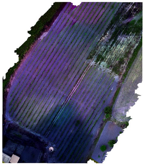
Figure 29.
Multispectral orthomap generated from images obtained using MicaSense camera. Distance between two points is approximately 0.2 m.
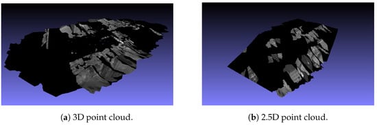
Figure 30.
Multispectral point cloud models generated from the processing of imagery obtained from MicaSense camera.
4.3. Thermal Product
Lastly, the generation of models based on thermal images has not seen great emphasis, as these images often possess a low density of distinct features which increases the difficulty of the detection and matching of features between images. Therefore, a method was developed to generate models using thermal images.
Here a Flir Vue Pro R camera was used that allows the capture of accurate and calibrated thermal images along with radiometric data from aerial platforms enabling it to be used to assist in precision agriculture.
The thermal image is extracted using a FLIR image extractor where the raw data of the thermal sensors can be extracted from the metadata of the input image [138]. The input image and the thermal sensor values are converted to temperatures and stored in a created image. The metadata of the original image is copied to the processed image. The processed thermal images are then stored in a different folder to be used later.
Following the extraction of thermal data, the original images follow the standard workflow of the program. The metadata is extracted, and the features are detected and matched between neighboring images. At this point, the image set is replaced by the processed thermal image set. Therefore, the original images are placed in a backup folder, and the thermal images take the place of the original images.
The switch of image set is done here because, as mentioned before, thermal images often present a low density of distinct features, so the matching of features becomes difficult. The intention with the switch of image set is to tell the program to use the features detected and matched of the original data set on the thermal images. As the creation of tracks only require the information regarding the features and matches of the images to create tracks and the reconstruction step expects the identifier of each image which are stored in the tracks manager generated by the track creation step, the switch of image set does not affect any of the mentioned steps. Following the reconstruction step, both sets of images, original and processed thermal images, have distortions removed as is required for the succeeding steps. The reason to undistort both image sets is that the densification requires the removal of distortion from the images to compute correctly the depth maps of each image. Additionally, the thermal images currently being used by the program are undistorted first, and the original images are undistorted afterward, placing the undistorted thermal images on the backup folder.
The original undistorted images are then used for the following steps, namely, the densification and meshing of the model. In the following step, the texturing, both image sets are switched once more. The reason for this switch is to texture the mesh using the processed thermal images. Afterward, the standard workflow is followed, as the GNSS coordinates used to georeference the model are equivalent on both image sets.
The interchanging between original imagery and thermal imagery allowed for the reconstruction of a thermal model, using the original image set to build the model and later textured using the thermal images.
The thermal dataset is composed of 321 images captured from the Flir Vue Pro R camera at approximately 313 m high. With images being taken roughly 20 m apart, allowing for an overlapping ratio of approximately 75%. The image set follows the standard reconstruction workflow with the modifications on the corresponding steps mentioned above. The result is displayed in Figure 31 and Figure 32.
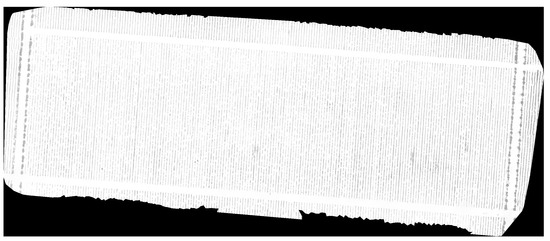
Figure 31.
Orthomap generated from thermal images. On average, a distance of 0.01 m is present between two consecutive points.
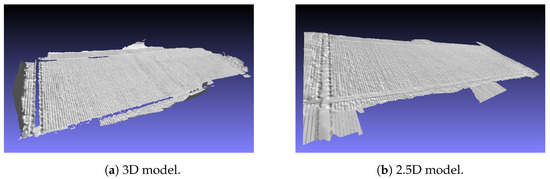
Figure 32.
Models generated from thermal images.
5. Discussion
In this paper, an overview of a 3D model creation system was studied using aerial images collected using UAVs. Three types of images were used: RGB, Multispectral, and Thermal. The first image set, the RGB, can be captured using a regular camera or smartphone, and therefore, the most common type of image is composed of three visible bands of the electromagnetic spectrum. In the second image set, the set is composed of images of five bands: three of the visible spectrum (red, green, and blue) and two of the invisible spectrum (near-infrared and red edge). For the final model, near-infrared images were used in order to build a thermal model of the surveyed region.
Using the system developed by [4], Each image set was introduced into the system, and its steps were carefully analyzed to understand the processes that affect the images and create a 3D model. Section 3 gives a detailed insight into the implemented method in the different steps of the system as well as other possible implementations in literature developed by other authors. The comparison between the systems is highlighted in Table 5.
Table 5.
Comparison between developed systems.
From this study, a conclusion was reached that different types of image sets do not follow the same workflow, and small modifications were implemented. In the case of the Multispectral image set, it followed the same workflow as that of the RGB, and then, it took a different processing path, where images of different bands were integrated into the model by comparing with images of the current band through homography, before joining back the path of the RGB workflow.
Additionally, an innovative mapping technique using thermal images was proposed as no such method was implemented in the developed system by [4], and no open-source tool was found. As these images often possess lower distinguishing features, the implemented workflow was adapted to allow the processing of the near-infrared images before analyzing the thermal data.
However, due to the current situation, the accuracy of the created models cannot be verified as it would require field survey measurements to be taken and compared to the same measurements of the model. For this, an authorization to the survey site is required that we do not possess at the moment.
All in all, the models and orthomaps obtained were extremely satisfactory, as most objects present in the real world and captured during the survey were successfully reconstructed in our experiments. Furthermore, the georeferenced models created presented excellent overlapping when displayed over google maps or interactive maps like Leaflet (Figure 33).
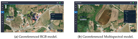
Figure 33.
Georeferenced model overlap with Leaflet interactive map. This platform was developed by [139,140].
However, future improvements are necessary. As it can be seen on the 3D and 2.5D models in the (single band and) multispectral experimental results, the models are not fully covered with texture patches obtained using the images, contrary to the results obtained using RGB and Thermal sets. It is still unclear to us why this happens, and further investigations are required. On the other hand, future surveys are required to test the robustness of the developed system. Additionally, a joint effort is being made with the developers of [4] regarding the integration of the proposed thermal mapping technique.
6. Conclusions
In this paper, an overview of an automated system to create outdoor models using aerial images collected using UAVs was conducted. A brief history of previous works and their methods is introduced, in order to give some background on the importance of shaped outdoor models in scientific fields that require mapping.
A detailed analysis is carried out on each step of a workflow based on OpenDroneMap and the processes through which the input images undergo to produce a map as the final product. For each step, an introduction of previous relevant works is displayed as well as the categories into which the algorithms can be divided. The output of each stage is used as the input of the succeeding process.
Finally, the workflow is applied to different types of datasets.
The most popular type of dataset, comprising RGB images, was used to generate the most digital models, as the cameras used to obtained such imagery are common and can be acquired using a regular camera/smartphone.
The second type of dataset was the multispectral images, where images were collected using a MicaSense camera. This camera is able to capture images on five different bands, red, green, and blue, from the visible spectrum, and near-infrared and red edge, from the invisible spectrum. Two paths were taken with this dataset, the computation of models using a single band and the combination of all the bands. Although the generated model was pretty similar in terms of mesh, the patch-based texture algorithm appeared to have suffered some difficulties. It can be stated though that the multispectral model computed using the combination of bands appears to display bigger texture patches when compared to the single-band model in both, 3D and 2.5D models. Furthermore, it should also be highlighted the resolution of the ortho map generated with all bands compared to the ortho map of the single band.
In the last dataset, thermal images were used. Due to a non-existent single open-source tool that allowed the processing of thermal images and the complications of Structure from Motion algorithms in generating products for thermal imagery, because of a low amount of distinct features and the homogeneity of outdoor environments, a strategy was devised to generate thermal models.
In summary, at the time of the writing of this paper, no literature was found that addressed in detail the computer vision processes used for mapping from image sets. The developed system, based on the work of OpenDroneMap, implements the principles of Structure from Motion to generate sparse models from aerial images, Multi-View Stereopsis to build dense models based on the sparse model, Poisson Reconstruction to compute the model’s mesh, and a patch-based texture model generated and attached to each mesh’s surface. Along with a few adjustments, the system allows the processing of RGB, multispectral, and thermal images and produces their respective models.
Author Contributions
Conceptualization, A.V., J.P.M.-C. and P.T.; Methodology, A.V., J.P.M.-C. and P.T.; Software, A.V., J.P.M.-C. and P.T.; Validation, A.V., J.P.M.-C., P.T., F.M. and N.C.G.; Investigation, A.V., J.P.M.-C. and P.T.; Resources, D.P. and F.A.; Writing—original draft preparation, A.V.; Writing—review and editing, A.V., J.P.M.-C., P.T., D.P., F.A., F.M., N.C.G. and A.M.; Supervision, J.P.M.-C. and A.M. All authors have read and agreed to the published version of the manuscript.
Funding
This project was partially funded by AI4RealAg project. The goal of the AI4RealAg project is to develop an intelligent knowledge extraction system, based in Artificial Intelligence and Data Science, to increase sustainable agricultural production. The project is financed by Portugal 2020, under the Lisbon’s Regional Operational Programme and the Competitiveness and Internationlization Operational Programme, worth 1.573.672.61 euros, from the European Regional Development Fund. This work was also partially funded by the Portuguese Fundação para a Ciência e a Tecnologia (FCT) under Project UIDB/04111/2020, Project foRESTER PCIF/SSI/0102/2017, Project IF/00325/2015, and Project UIDB/00066/2020.
Institutional Review Board Statement
Not applicable.
Informed Consent Statement
Not applicable.
Data Availability Statement
The dataset used in this work can be accessed at https://multispectral-datanet.com (accessed on 15 May 2021).
Acknowledgments
The authors would like to thank the COPELABS, Beyond Vision Research Group and PDMFC Research and Development Team.
Conflicts of Interest
The authors declare no conflict of interest.
References
- Max Roser and Hannah Ritchie—“Technological Progress”. Published online at OurWorldInData.org. 2013. Available online: https://ourworldindata.org/technological-progress (accessed on 3 February 2021).
- Lowe, D.G. Object Recognition From Local Scale-Invariant Features. In Proceedings of the Seventh IEEE International Conference on Computer Vision, Kerkyra, Greece, 20–27 September 1999; Volume 2, pp. 1150–1157. [Google Scholar] [CrossRef]
- Lowe, D.G. Distinctive Image Features From Scale-Invariant Keypoints. Int. J. Comput. Vis. 2004, 60, 91–110. [Google Scholar] [CrossRef]
- OpenDroneMap Authors ODM—A Command Line Toolkit to Generate Maps, Point Clouds, 3D Models and DEMs from Drone, Balloon or Kite Images. OpenDroneMap/ODM GitHub Page 2020. Available online: https://github.com/OpenDroneMap/ODM (accessed on 2 October 2020).
- Administrator, Agisoft Metashape. Available online: https://www.agisoft.com/ (accessed on 20 October 2020).
- Administrator, Pix4D. Available online: https://www.pix4d.com/ (accessed on 25 October 2020).
- Administrator, Arc3D. Available online: https://homes.esat.kuleuven.be/~visit3d/webservice/v2/index.php (accessed on 30 October 2020).
- Administrator, Bundler. Available online: http://www.cs.cornell.edu/~snavely/bundler/ (accessed on 1 November 2020).
- Casella, V.; Chiabrando, F.; Franzini, M.; Manzino, A.M. Accuracy Assessment of a UAV Block by Different Software Packages, Processing Schemes and Validation Strategies. ISPRS Int. J. Geo-Inf. 2020, 9, 164. [Google Scholar] [CrossRef]
- Neitzel, F.; Klonowski, J. Mobile 3D mapping with a low-cost UAV system. Int. Arch. Photogramm. Remote Sens. Spat. Inf. Sci. 2011, XXXVIII-1/C22, 39–44. [Google Scholar] [CrossRef]
- Sona, G.; Pinto, L.; Pagliari, D.; Passoni, D.; Gini, R. Experimental analysis of different software packages for orientation and digital surface modelling from UAV images. Earth Sci. Inform. 2014, 7, 97–107. [Google Scholar] [CrossRef]
- Wang, T.; Zeng, J.; Liu, D.-J.; Yang, L.-Y. Fast stitching of DOM based on small UAV. J. Inf. Optim. Sci. 2017, 38, 1211–1219. [Google Scholar] [CrossRef]
- Karantanellis, E.; Arav, R.; Dille, A.; Lippl, S.; Marsy, G.; Torresani, L.; Elberink, S.O. Evaluating the Quality of Photogrammetric Point-Clouds in Challenging Geo-Environments–A Case Study in An Alpine Valley. Int. Arch. Photogramm. Remote Sens. Spat. Inf. Sci. 2020, XLIII-B2-2020, 1099–1105. [Google Scholar] [CrossRef]
- Guimarães, N.; Pádua, L.; Adão, T.; Hruška, J.; Peres, E.; Sousa, J.J. VisWebDrone: A Web Application for UAV Photogrammetry Based on Open-Source Software. ISPRS Int. J. Geo-Inf. 2020, 9, 679. [Google Scholar] [CrossRef]
- Schütz, M. Potree: Rendering Large Point Clouds in Web Browsers. Ph.D. Thesis, Institut für Computergraphik und Algorithmen, Wien, Austria, 2016. [Google Scholar]
- Schütz, M.; Ohrhallinger, S.; Wimmer, M. Fast Out-of-Core Octree Generation for Massive Point Clouds. Comput. Graph. Forum 2020, 39, 155–167. [Google Scholar] [CrossRef]
- Crickard, P. Leaflet.js Essentials; Packt Publishing: Birmingham, UK, 2014. [Google Scholar]
- Hrushchak, Y. Visual Localization for Iseauto Using Structure From Motion. MSc Thesis, Tallinn University of Technology, Tallinn, Estonia, 2019. [Google Scholar]
- Mapillary, Opensfm. Available online: Https://Github.Com/Mapillary/Opensfm#Getting-Started (accessed on 15 October 2020).
- Administrator, Camera Distortion. Available online: http://gazebosim.org/tutorials?tut=camera_distortion (accessed on 12 October 2020).
- Frontera, F.; Smith, M.J.; Marsh, S. Preliminary Investigation into the Geometric Calibration of the Micasense Rededge-M Multispectral Camera. ISPRS-Int. Arch. Photogramm. Remote Sens. Spat. Inf. Sci. 2020, Xliii-B2-2020, 17–22. [Google Scholar] [CrossRef]
- Bay, H.; Ess, A.; Tuytelaars, T.; Gool, L.V. Speeded-Up Robust Features (SURF). Comput. Vis. Image Underst. 2008, 110, 346–359. [Google Scholar] [CrossRef]
- Rublee, E.; Rabaud, V.; Konolige, K.; Bradski, G. ORB: An Efficient Alternative to Sift or Surf. In Proceedings of the 2011 International Conference on Computer Vision, Barcelona, Spain, 6–13 November 2011; pp. 2564–2571. [Google Scholar] [CrossRef]
- Koenderink, J.J. The Structure of Images. Biol. Cybern. 1984, 50, 363–370. [Google Scholar] [CrossRef]
- Lindeberg, T. Scale-Space Theory: A Basic Tool for Analysing Structures At Different Scales. J. Appl. Stat. 1994, 21, 224–270. [Google Scholar] [CrossRef]
- Mikolajczyk, K.; Schmid, C. An Affine Invariant Interest Point Detector. In Computer Vision—Eccv 2002, Proceedings of the 7th European Conference on Computer Vision, Copenhagen, Denmark, 28–31 May 2002; Lecture Notes in Computer Science; Heyden, A., Sparr, G., Nielsen, M., Johansen, P., Eds.; Springer: Berlin/Heidelberg, Germany, 2002; Volume 2350. [Google Scholar] [CrossRef]
- Huang, M.; Mu, Z.; Zeng, H.; Huang, H. A Novel Approach for Interest Point Detection via Laplacian-of-Bilateral Filter. J. Sens. 2015, 2015, 685154. [Google Scholar] [CrossRef]
- Brown, M.; Lowe, D. Invariant Features from Interest Point Groups. In Proceedings of the British Machine Conference; Marshall, D., Rosin, P.L., Eds.; Bmva Press: Dundee, UK, 2002; pp. 23.1–23.10. [Google Scholar] [CrossRef]
- Harris, C.; Stephens, M. A Combined Corner and Edge Detector. In Proceedings of the 4th Alvey Vision Conference, Manchester, UK, 31 August–2 September 1988; pp. 147–151. [Google Scholar]
- Schmid, C.; Mohr, R. Local Grayvalue Invariants for Image Retrieval. IEEE Trans. Pattern Anal. Mach. Intell. 1997, 19, 530–535. [Google Scholar] [CrossRef]
- Edelman, S.; Intrator, N.; Poggio, T. Complex Cells and Object Recognition; NIPS*97, Visual Processing, 1997, Unpublished.
- Eichhorn, J.; Chapelle, O. Object Categorization with SVM: Kernels for Local Features; Max Planck Institute for Biological Cybernetics: Baden-Württemberg, Germany, 2004. [Google Scholar]
- Csurka, G.; Dance, C.; Fan, L.; Willamowski, J.; Bray, C. Visual Categorization with Bags of Keypoints. Workshop Stat. Learn. Comput. Vis. 2004, 1, 1–2. [Google Scholar]
- O’hara, S.; Draper, B. Introduction to the Bag of Features Paradigm for Image Classification and Retrieval. arXiv 2011, arXiv:1101.3354. [Google Scholar]
- Muja, M.; Lowe, D.G. Fast Approximate Nearest Neighbors with Automatic Algorithm Configuration. In VISAPP 2009, Proceedings of the 4th International Conference on Computer Vision Theory and Applications, Lisbon, Portugal, 5–8 February 2009; Volume 1, pp. 331–340.
- Friedman, J.H.; Bentley, J.L.; Finkel, R.A. An Algorithm for Finding Best Matches in Logarithmic Expected Time. ACM Trans. Math. Softw. 1977, 3, 209–226. [Google Scholar] [CrossRef]
- Beis, J.S.; Lowe, D.G. Shape Indexing Using Approximate Nearest-Neighbour Search in High-Dimensional Spaces. In Proceedings of the 1997 Conference on Computer Vision and Pattern Recognition (Cvpr ’97), San Juan, PR, USA, 17–19 June 1997; pp. 1000–1006. [Google Scholar]
- Hough, P.V.C. Method and Means for Recognizing Complex Patterns. U.S. Patent 3,069,654, 18 December 1962. [Google Scholar]
- Ballard, D.H. Generalizing the Hough Transform To Detect Arbitrary Shapes. Pattern Recognit. 1981, 13, 111–122. [Google Scholar] [CrossRef]
- Andrew, A.; Eric, W.; Grimson, L.; Lazano-Pérez, T.; Huttenlocher, D.P. Object Recognition By Computer: The Role of Geometric Constraints, Mit Press, Cambridge, Mass., 1990, Hard Cover, Xv 512 Pp. (£40.50). Robotica 1992, 10, 475. [Google Scholar] [CrossRef]
- Lowe, D.G. Local Feature View Clustering for 3d Object Recognition. In Proceedings of the 2001 IEEE Computer Society Conference on Computer Vision and Pattern Recognition. CVPR 2001, Kauai, HI, USA, 8–14 December 2001; p. 1. [Google Scholar] [CrossRef]
- Havlena, M.; Schindler, K. Vocmatch: Efficient Multiview Correspondence for Structure from Motion. In Computer Vision—Eccv 2014, Proceedings of the 13th European Conference, Zurich, Switzerland, 6–12 September 2014; Lecture Notes in Computer Science; Fleet, D., Pajdla, T., Schiele, B., Tuytelaars, T., Eds.; Springer: Cham, Switzerland, 2014; Volume 8691. [Google Scholar] [CrossRef]
- Levenberg, K. A Method for the Solution of Certain Non-Linear Problems In Least Squares. Q. Appl. Math. 1944, 2, 164–168. [Google Scholar] [CrossRef]
- Kataria, R.; DeGol, J.; Hoiem, D. Improving Structure from Motion with Reliable Resectioning. In Proceedings of the 2020 International Conference on 3D Vision (3DV), Fukuoka, Japan, 25–28 November 2020; pp. 41–50. [Google Scholar] [CrossRef]
- Adorjan, M. OpenSfM: A Collaborative Structure-From-Motion System. Ph.D. Thesis, Vienna University of Technology, Vienna, Austria, 2016. [Google Scholar]
- Wu, F.; Wei, H.; Wang, X. Correction of image radial distortion based on division model. Opt. Eng. 2017, 56, 013108. [Google Scholar] [CrossRef]
- Furukawa, Y.; Hernández, C. Multi-View Stereo: A Tutorial. In Foundations and TrendsR in Computer Graphics and Vision; Now Publishers Inc.: Hanover, MA, USA, 2013; Volume 9, pp. 1–148. [Google Scholar]
- Furukawa, Y.; Ponce, J. Accurate, Dense, and Robust Multiview Stereopsis. IEEE Trans. Pattern Anal. Mach. Intell. 2010, 32, 1362–1376. [Google Scholar] [CrossRef] [PubMed]
- Seitz, S.M.; Dyer, C.R. Photorealistic Scene Reconstruction By Voxel Coloring. Int. J. Comput. Vis. 1999, 35, 151–173. [Google Scholar] [CrossRef]
- Vogiatzis, G.; Esteban, C.H.; Torr, P.H.; Cipolla, R. Multiview Stereo via Volumetric Graph-Cuts and Occlusion Robust Photo-Consistency. IEEE Trans. Pattern Anal. Mach Intell. 2007, 29, 2241–2246. [Google Scholar] [CrossRef]
- Sinha, S.N.; Mordohai, P.; Pollefeys, M. Multi-View Stereo via Graph Cuts on the Dual of an Adaptive Tetrahedral Mesh. In Proceedings of the IEEE International Conference on Computer Vision, Rio de Janeiro, Brazil, 14–21 October 2007; pp. 1–8. [Google Scholar] [CrossRef]
- Shen, S. Accurate Multiple View 3d Reconstruction Using Patch-Based Stereo for Large-Scale Scenes. IEEE Trans. Image Process. 2013, 22, 1901–1914. [Google Scholar] [CrossRef] [PubMed]
- Faugeras, O.; Keriven, R. Variational Principles, Surface Evolution, Pdes, Level Set Methods and the Stereo Problem. IEEE Trans. Image Process. 1998, 7, 336–344. [Google Scholar] [CrossRef]
- Esteban, C.H.; Schmitt, F. Silhouette and Stereo Fusion for 3D Object Modeling. Comput. Vis. Image Underst. 2004, 96, 367–392. [Google Scholar] [CrossRef]
- Hiep, V.H.; Keriven, R.; Labatut, P.; Pons, J.P. Towards High-Resolution Large-Scale Multi-View Stereo. In Proceedings of the 2009 IEEE Computer Society Conference on Computer Vision And Pattern Recognition, Miami, FL, USA, 20–25 June 2009; pp. 1430–1437. [Google Scholar] [CrossRef]
- Kolev, K.; Cremers, D. Integration of Multiview Stereo And Silhouettes Via Convex Functionals on Convex Domains. In Computer Vision—Eccv 2008: 10th European Conference on Computer Vision, Marseille, France, 12–18 October 2008, Proceedings, Part I; Lecture Notes in Computer Science, Volume 5302; Forsyth, D., Torr, P., Zisserman, A., Eds.; Springer: Berlin/Heidelberg, Germany, 2008. [Google Scholar] [CrossRef]
- Goesele, M.; Curless, B.; Seitz, S.M. Multi-View Stereo Revisited. In Proceedings of the 2006 IEEE Computer Society Conference on Computer Vision and Pattern Recognition (CVPR’06), New York, NY, USA, 17–22 June 2006; pp. 2402–2409. [Google Scholar] [CrossRef]
- Merrell, P.; Akbarzadeh, A.; Wang, L.; Mordohai, P.; Frahm, J.M.; Yang, R.; Nistér, D.; Pollefeys, M. Real-Time Visibility-Based Fusion of Depth Maps. In Proceedings of the 2007 IEEE 11th International Conference on Computer Vision, Rio de Janeiro, Brazil, 14–21 October 2007; pp. 1–8. [Google Scholar] [CrossRef]
- Fuhrmann, S.; Goesele, M. Fusion of Depth Maps with Multiple Scales. ACM Trans. Graph. 2011, 30, 148. [Google Scholar] [CrossRef]
- Lhuillier, M.; Quan, L. A Quasi-Dense Approach To Surface Reconstruction from Uncalibrated Images. IEEE Trans. Pattern Anal. Mach. Intell. 2005, 27, 418–433. [Google Scholar] [CrossRef] [PubMed]
- Goesele, M.; Snavely, N.; Curless, B.; Hoppe, H.; Seitz, S.M. Multi-View Stereo for Community Photo Collections. In Proceedings of the 2007 IEEE 11th International Conference on Computer Vision, Rio de Janeiro, Brazil, 14–21 October 2007; pp. 1–8. [Google Scholar] [CrossRef]
- Cernea, D. Openmvs: Multi-View Stereo Reconstruction Library. 2020. Available online: https://github.com/cdcseacave/openMVS (accessed on 10 February 2021).
- Barnes, C.; Shechtman, E.; Finkelstein, A.; Goldman, D.B. Patchmatch: A Randomized Correspondence Algorithm for Structural Image Editing. ACM Trans. Graph. 2009, 28, 24. [Google Scholar] [CrossRef]
- Li, J.; Li, E.; Chen, Y.; Xu, L.; Zhang, Y. Bundled Depth-Map Merging for Multi-View Stereo. In Proceedings of the 2010 IEEE Computer Society Conference on Computer Vision and Pattern Recognition, San Francisco, CA, USA, 13–18 June 2010; pp. 2769–2776. [Google Scholar] [CrossRef]
- Bleyer, M.; Rhemann, C.; Rother, C. Patchmatch Stereo-Stereo Matching with Slanted Support Windows. In Jesse Hoey, Stephen Mckenna and Emanuele Trucco, Proceedings of the British Machine Vision Conference; Bmva Press: Dundee, UK, 2011; pp. 14.1–14.11. [Google Scholar] [CrossRef]
- Jamwal, N.; Jindal, N.; Singh, K. A Survey on Depth Map Estimation Strategies. In Proceedings of the International Conference on Signal Processing (ICSP 2016), Vidisha, India, 7–9 November 2016; pp. 1–5. [Google Scholar] [CrossRef]
- Pustelnik, N.; Laurent, C. Proximity Operator of A Sum of Functions; Application to Depth Map Estimation. IEEE Signal Process. Lett. 2017, 24, 1827–1831. [Google Scholar] [CrossRef][Green Version]
- Choe, J.; Joo, K.; Imtiaz, T.; Kweon, I.S. Volumetric Propagation Network: Stereo-Lidar Fusion for Long-Range Depth Estimation. IEEE Robot. Autom. Lett. 2021, 6, 4672–4679. [Google Scholar] [CrossRef]
- Zheng, E.; Dunn, E.; Raguram, R.; Frahm, J.M. Efficient and Scalable Depthmap Fusion. In Proceedings of the British Machine Vision Conference 2012, Surrey, UK, 3–7 September 2012. [Google Scholar] [CrossRef]
- PDAL Contributors. PDAL Point Data Abstraction Library. 2018. Available online: https://doi.org/10.5281/zenodo.2556738 (accessed on 19 February 2021).
- Khatamian, A.; Arabnia, H.R. Survey on 3D Surface Reconstruction. J. Inf. Process. Syst. 2016, 12, 338–357. [Google Scholar] [CrossRef]
- Digne, J.; Cohen-Steiner, D.; Alliez, P.; De Goes, F.; Desbrun, M. Feature-Preserving Surface Reconstruction and Simplification from Defect-Laden Point Sets. J. Math. Imaging Vis. 2014, 48, 369–382. [Google Scholar] [CrossRef]
- DeCarlo, D.; Metaxas, D. Blended Deformable Models. IEEE Trans. Pattern Anal. Mach. Intell. 1996, 18, 443–448. [Google Scholar] [CrossRef]
- Terzopoulos, D.; Witkin, A.; Kass, M. Constraints on Deformable Models:Recovering 3d Shape and Nonrigid Motion. Artif. Intell. 1988, 36, 91–123. [Google Scholar] [CrossRef]
- Taubin, G. An Improved Algorithm for Algebraic Curve and Surface Fitting. In Proceedings of the 1993 4th International Conference on Computer Vision, Berlin, Germany, 11–14 May 1993; pp. 658–665. [Google Scholar] [CrossRef]
- Szeliski, R.; Tonnesen, D.; Terzopoulos, D. Modeling Surfaces of Arbitrary Topology with Dynamic Particles. In Proceedings of the IEEE Conference on Computer Vision and Pattern Recognition, New York, NY, USA, 15–17 June 1993; pp. 82–87. [Google Scholar] [CrossRef]
- Hoffmann, C.; Hopcroft, J. The Geometry of Projective Blending Surfaces. Artif. Intell. 1988, 37, 357–376. [Google Scholar] [CrossRef][Green Version]
- Muraki, S. Volumetric Shape Description of Range Data Using “Blobby Model”. In SIGGRAPH ’91: Proceedings of the 18th Annual Conference on Computer Graphics and Interactive Techniques; Association for Computing Machinery: New York, NY, USA, 1991; pp. 227–235. [Google Scholar] [CrossRef]
- Hanson, A.J. Hyperquadrics: Smoothly Deformable Shapes with Convex Polyhedral Bounds. Comput. Vis. Graph. Image Process. 1988, 44, 191–210. [Google Scholar] [CrossRef]
- Terzopoulos, D.; Metaxas, D. Dynamic 3d Models with Local and Global Deformations: Deformable Superquadrics. IEEE Trans. Pattern Anal. Mach. Intell. 1991, 13, 703–714. [Google Scholar] [CrossRef]
- Barr, A.H. Superquadrics and Angle-Preserving Transformations. IEEE Comput. Graph. Appl. 1981, 1, 11–23. [Google Scholar] [CrossRef]
- O’Donnell; Boult; Fang, X.-S.; Gupta. The Extruded Generalized Cylinder: A Deformable Model for Object Recovery. In Proceedings of the 1994 IEEE Conference on Computer Vision and Pattern Recognition, Seattle, WA, USA, 21–23 June 1994; pp. 174–181. [Google Scholar] [CrossRef]
- Marr, D.; Nishihara, H.K. Representation and Recognition of the Spatial Organization of Three-Dimensional Shapesproc. Proc. R. Soc. Lond. Ser. B Biol. Sci. 1978, 200, 269–294. [Google Scholar] [CrossRef]
- Hoppe, H.; DeRose, T.; Duchamp, T.; McDonald, J.; Stuetzle, W. Surface Reconstruction from Unorganized Point Clouds. In SIGGRAPH ’92: Proceedings of the 19th Annual Conference on Computer Graphics and Interactive Techniques; Association for Computing Machinery: New York, NY, USA, 1992. [Google Scholar]
- Klein, R. Voronoi Diagrams and Delaunay Triangulations. In Encyclopedia of Algorithms; Kao, M.Y., Ed.; Springer: New York, NY, USA, 2016. [Google Scholar] [CrossRef]
- Amenta, N.; Bern, M.; Kamvysselis, M. A New Voronoi-Based Surface Reconstruction Algorithm. In SIGGRAPH ’98: Proceedings of the 25th Annual Conference on Computer Graphics and Interactive Techniques; Association for Computing Machinery: New York, NY, USA, 1998; pp. 415–421. [Google Scholar] [CrossRef]
- Amenta, N.; Choi, S.; Kolluri, R.K. The Power Crust. In SMA ’01: Proceedings of the Sixth ACM Symposium on Solid Modeling and Applications; Association for Computing Machinery: New York, NY, USA, 2001; pp. 249–266. [Google Scholar] [CrossRef]
- Bernardini, F.; Mittleman, J.; Rushmeier, H.; Silva, C.; Taubin, G. The Ball-Pivoting Algorithm for Surface Reconstruction. IEEE Trans. Vis. Comput. Graph. 1999, 5, 349–359. [Google Scholar] [CrossRef]
- Gopi, M.; Krishnan, S.; Silva, C.T. Surface Reconstruction Based on Lower Dimensional Localized Delaunay Triangulation. Comput. Graph. Forum 2000, 19, 467–478. [Google Scholar] [CrossRef]
- Gopi, M.; Krishnan, S. A Fast and Efficient Projection-Based Approach for Surface Reconstruction. In Proceedings of the XV Brazilian Symposium on Computer Graphics and Image Processing, Fortaleza, Brazil, 10 October 2002. [Google Scholar] [CrossRef]
- Dinh, H.Q.; Turk, G.; Slabaugh, G. Reconstructing Surfaces Using Anisotropic Basis Functions. In Proceedings of the Eighth IEEE International Conference on Computer Vision. ICCV 2001, Vancouver, BC, Canada, 7–14 July 2001; Volume 2, pp. 606–613. [Google Scholar] [CrossRef]
- Huang, H.; Li, D.; Zhang, H.; Ascher, U.; Cohen-Or, D. Consolidation of Unorganized Point Clouds for Surface Reconstruction. ACM Trans. Graph. 2009, 28, 1–7. [Google Scholar] [CrossRef]
- Alexa, M.; Behr, J.; Cohen-Or, D.; Fleishman, S.; Levin, D.; Silva, C.T. Computing and Rendering Point Set Surfaces. IEEE Trans. Vis. Comput. Graph. 2003, 9, 3–15. [Google Scholar] [CrossRef]
- Öztireli, A.C.; Guennebaud, G.; Gross, M. Feature Preserving Point Set Surfaces Based on Non-Linear Kernel Regression. Comput. Graph. Forum 2009, 28, 493–501. [Google Scholar] [CrossRef]
- Kazhdan, M.; Bolitho, M.; Hoppe, H. Poisson Surface Reconstruction. In SGP ’06: Proceedings of the Fourth Eurographics Symposium on Geometry Processing; Eurographics Association: Goslar, Germany, 2006; pp. 61–70. [Google Scholar]
- Li, X.; Wan, W.; Cheng, X.; Cui, B. An Improved Poisson Surface Reconstruction Algorithm. In Proceedings of the 2010 International Conference on Audio, Language and Image Processing, Shanghai, China, 23–25 November 2010; pp. 1134–1138. [Google Scholar] [CrossRef]
- Bolitho, M.; Kazhdan, M.; Burns, R.; Hoppe, H. Parallel Poisson Surface Reconstruction. In Advances In Visual Computing: 5th International Symposium, ISVC 2009, Las Vegas, NV, USA, 30 November–2 December 2009, Proceedings, Part I; Lecture Notes in Computer Science, Volume 5875; Bebis, G., Boyle, R., Parvin, B., Koracin, D., Kuno, Y., Wang, J., Pajarola, R., Lindstrom, P., Hinkenjann, A., Encarnação, M.L., et al., Eds.; Springer: Berlin/Heidelberg, Germany, 2009. [Google Scholar] [CrossRef]
- Kazhdan, M.; Maloney, A. Poissonrecon. Available online: Https://Github.Com/Mkazhdan/Poissonrecon (accessed on 2 March 2021).
- Lorensen, W.E.; Cline, H.E. Marching Cubes: A High Resolution 3d Surface Construction Algorithm. In SIGGRAPH ’87: Proceedings of the 14th Annual Conference on Computer Graphics and Interactive Techniques; Association for Computing Machinery: New York, NY, USA, 1987; pp. 163–169. [Google Scholar] [CrossRef]
- Fletcher, C.A.J. Computational Galerkin Methods; Springer Series in Computational Physics; Springer: Berlin/Heidelberg, Germany, 1984. [Google Scholar] [CrossRef]
- Kazhdan, M.; Hoppe, H. Screened poisson surface reconstruction. ACM Trans. Graph. 2013, 32, 1–13. [Google Scholar] [CrossRef]
- Kazhdan, M.; Hoppe, H. An Adaptive Multi-Grid Solver for Applications in Computer Graphics. Comput. Graph. Forum 2019, 38, 138–150. [Google Scholar] [CrossRef]
- Kazhdan, M.; Chuang, M.; Rusinkiewicz, S.; Hoppe, H. Poisson Surface Reconstruction with Envelope Constraints. Comput. Graph. Forum 2020, 39, 173–182. [Google Scholar] [CrossRef]
- Höllig, K.; Reif, U.; Wipper, J. Weighted Extended B-Spline Approximation of Dirichlet Problems. SIAM J. Numer. Anal. 2001, 39, 442–462. [Google Scholar] [CrossRef]
- Elizabeth, Full 3D vs. 2.5D Processing. Available online: https://support.dronesmadeeasy.com/hc/en-us/articles/207855366-Full-3D-vs-2-5D-Processing (accessed on 8 March 2021).
- Li, S.; Xiao, X.; Guo, B.; Zhang, L. A Novel OpenMVS-Based Texture Reconstruction Method Based on the Fully Automatic Plane Segmentation for 3D Mesh Models. Remote Sens. 2020, 12, 3908. [Google Scholar] [CrossRef]
- Fu, Y.; Yan, Q.; Yang, L.; Liao, J.; Xiao, C. Texture Mapping for 3D Reconstruction with RGB-D Sensor. In Proceedings of the 2018 IEEE/CVF Conference on Computer Vision and Pattern Recognition, Salt Lake City, UT, USA, 18–23 June 2018; pp. 4645–4653. [Google Scholar] [CrossRef]
- Kehl, W.; Navab, N.; Ilic, S. Coloured Signed Distance Fields for Full 3D Object Reconstruction. BMVC. 2014. Available online: http://www.bmva.org/bmvc/2014/papers/paper012/index.html (accessed on 20 March 2021).
- Callieri, M.; Cignoni, P.; Corsini, M.; Scopigno, R. Masked photo blending: Mapping dense photographic data set on high-resolution sampled 3D models. Comput. Graph. 2008, 32, 464–473. [Google Scholar] [CrossRef]
- Fausto, B.; Martin, I.M.; Rushmeier, H. High-Quality Texture Reconstruction from Multiple Scans. IEEE Trans. Vis. Comput. Graph. 2001, 7, 318–332. [Google Scholar]
- Hoegner, L.; Stilla, U. Automatic 3D Reconstruction and Texture Extraction for 3D Building Models from Thermal Infrared Image Sequences. Quant. InfraRed Thermogr. 2016. [Google Scholar] [CrossRef]
- Bi, S.; Kalantari, N.K.; Ramamoorthi, R. Patch-based optimization for image-based texture mapping. ACM Trans. Graph. 2017, 36, 1–11. [Google Scholar] [CrossRef]
- Zhao, H.; Li, X.; Ge, H.; Lei, N.; Zhang, M.; Wang, X.; Gu, X. Conformal mesh parameterization using discrete Calabi flow. Comput. Aided Geom. Des. 2018, 63, 96–108. [Google Scholar] [CrossRef]
- Li, S.; Luo, Z.; Zhen, M.; Yao, Y.; Shen, T.; Fang, T.; Quan, L. Cross-Atlas Convolution for Parameterization Invariant Learning on Textured Mesh Surface. In Proceedings of the 2019 IEEE/CVF Conference on Computer Vision and Pattern Recognition (CVPR), Long Beach, CA, USA, 15–20 June 2019; pp. 6136–6145. [Google Scholar] [CrossRef]
- Liu, L.; Ye, C.; Ni, R.; Fu, X.-M. Progressive parameterizations. ACM Trans. Graph. 2018, 37, 1–12. [Google Scholar] [CrossRef]
- Inzerillo, L.; Di Paola, F.; Alogna, Y. High Quality Texture Mapping Process Aimed at the Optimization of 3D Structured Light Models. ISPRS-Int. Arch. Photogramm. Remote Sens. Spat. Inf. Sci. 2019, XLII-2/W9, 389–396. [Google Scholar] [CrossRef]
- Eisemann, M.; De Decker, B.; Magnor, M.; Bekaert, P.; De Aguiar, E.; Ahmed, N.; C Theobalt, A. Sellent. Floating Textures. Comput. Graph. Forum 2008, 27, 409–418. [Google Scholar] [CrossRef]
- Aganj, E.; Monasse, P.; Keriven, R. Multi-view Texturing of Imprecise Mesh. In Computer Vision—ACCV 2009; Lecture Notes in Computer Science, Voumel 5995; Zha, H., Taniguchi, R., Maybank, S., Eds.; Springer: Berlin/Heidelberg, Germany, 2010. [Google Scholar] [CrossRef]
- Lempitsky, V.; Ivanov, D. Seamless Mosaicing of Image-Based Texture Maps. In Proceedings of the 2007 IEEE Conference on Computer Vision and Pattern Recognition, Minneapolis, MN, USA, 17–22 June 2007; pp. 1–6. [Google Scholar] [CrossRef]
- Gal, R.; Wexler, Y.; Ofek, E.; Hoppe, H.; Cohen-Or, D. Seamless Montage for Texturing Models. Comput. Graph. Forum 2010, 29, 479–486. [Google Scholar] [CrossRef]
- Allene, C.; Pons, J.P.; Keriven, R. Seamless image-based texture atlases using multi-band blending. In Proceedings of the 2008 19th International Conference on Pattern Recognition, Tampa, FL, USA, 8–11 December 2008; pp. 1–4. [Google Scholar] [CrossRef]
- Yang, Y.; Zhang, Y. A High-Realistic Texture Mapping Algorithm Based on Image Sequences. In Proceedings of the 2018 26th International Conference on Geoinformatics, Kunming, China, 28–30 June 2018; pp. 1–8. [Google Scholar] [CrossRef]
- Li, W.; Gong, H.; Yang, R. Fast Texture Mapping Adjustment via Local/Global Optimization. IEEE Trans. Vis. Comput. Graph. 2019, 25, 2296–2303. [Google Scholar] [CrossRef]
- Burt, P.J.; Adelson, E.H. A multiresolution spline with application to image mosaics. ACM Trans. Graph. 1983, 24, 217–236. [Google Scholar] [CrossRef]
- Pérez, P.; Gangnet, M.; Blake, A. Poisson image editing. ACM Trans. Graph. 2003, 22, 313–318. [Google Scholar] [CrossRef]
- Waechter, M.; Moehrle, N.; Goesele, M. Let There Be Color! Large-Scale Texturing of 3D Reconstructions. In Computer Vision—ECCV 2014: 13th European Conference, Zurich, Switzerland, 6–12 September 2014, Proceedings, Part V; Lecture Notes in Computer Science, Volume 8693; Fleet, D., Pajdla, T., Schiele, B., Tuytelaars, T., Eds.; Springer: Cham, Switzerland, 2014. [Google Scholar] [CrossRef]
- Waechter, M.; Moehrle, N.; Goesele, M. MVS-Texturing. 2014. Available online: https://github.com/nmoehrle/mvs-texturing (accessed on 30 March 2021).
- Geva, A. ColDet—3D Collision Detection Library. 2000. Available online: https://github.com/fougue/claudette (accessed on 28 March 2021).
- Sinha, S.N.; Steedly, D.; Szeliski, R.; Agrawala, M.; Pollefeys, M. Interactive 3D architectural modeling from unordered photo collections. ACM Trans. Graph. 2008, 27, 1–10. [Google Scholar] [CrossRef]
- Grammatikopoulos, L.; Kalisperakis, I.; Karras, G.; Petsa, E. Automatic Multi-View Texture Mapping of 3D Surface Projections. 2012. Available online: https://www.researchgate.net/publication/228367713_Automatic_multi-view_texture_mapping_of_3D_surface_projections (accessed on 23 March 2021).
- Guennebaud, G.; Jacob, B.; Capricelli, T.; Garg, R.; Hertzberg, C.; Holoborodko, P.; Lenz, M.; Niesen, J.; Nuentsa, D.; Steiner, B.; et al. Eigen v3. 2010. Available online: http://eigen.tuxfamily.org (accessed on 3 April 2021).
- GDAL/OGR Contributors, GDAL/OGR Geospatial Data Abstraction Software Library, Open Source Geospatial Foundation. 2021. Available online: https://gdal.org (accessed on 12 April 2021).
- Engineers, A.S.C. Glossary of the Mapping Sciences; American Society of Civil Engineers: Reston, VA, USA, 1994; ISBN 9780784475706. Available online: https://books.google.pt/books?id=jPVxSDzVRP0C (accessed on 15 April 2021).
- Smith, G.S. Digital Orthophotography and Gis, Green Mountain GeoGraphics, Ltd. Available online: https://proceedings.esri.com/library/userconf/proc95/to150/p124.html (accessed on 20 April 2021).
- Ritter, N.; Brown, E. Libgeotiff. 2020. Available online: https://github.com/OSGeo/libgeotiff (accessed on 20 April 2021).
- Salvado, A.B.; Mendonça, R.; Lourenço, A.; Marques, F.; Matos-Carvalho, J.P.; Campos, L.M.; Barata, J. Semantic Navigation Mapping from Aerial Multispectral Imagery. In Proceedings of the 2019 IEEE 28th International Symposium on Industrial Electronics (ISIE), Vancouver, BC, Canada, 12–14 June 2019; pp. 1192–1197. [Google Scholar] [CrossRef]
- Evangelidis, G.D.; Psarakis, E.Z. Parametric Image Alignment Using Enhanced Correlation Coefficient Maximization. IEEE Trans. Pattern Anal. Mach. Intell. 2008, 30, 1858–1865. [Google Scholar] [CrossRef]
- NationalDronesAu. Flir Image Extractor CLI. Available online: https://github.com/nationaldronesau/FlirImageExtractor (accessed on 1 May 2021).
- Pino, M.; Matos-Carvalho, J.P.; Pedro, D.; Campos, L.M.; Seco, J.C. UAV Cloud Platform for Precision Farming. In Proceedings of the 2020 12th International Symposium on Communication Systems, Networks and Digital Signal Processing (CSNDSP), Porto, Portugal, 20–22 July 2020; pp. 1–6. [Google Scholar] [CrossRef]
- Pedro, D.; Matos-Carvalho, J.P.; Azevedo, F.; Sacoto-Martins, R.; Bernardo, L.; Campos, L.; Fonseca, J.M.; Mora, A. FFAU—Framework for Fully Autonomous UAVs. Remote Sens. 2020, 12, 3533. [Google Scholar] [CrossRef]


Publisher’s Note: MDPI stays neutral with regard to jurisdictional claims in published maps and institutional affiliations. |
© 2021 by the authors. Licensee MDPI, Basel, Switzerland. This article is an open access article distributed under the terms and conditions of the Creative Commons Attribution (CC BY) license (https://creativecommons.org/licenses/by/4.0/).