Airborne LiDAR Point Cloud Processing for Archaeology. Pipeline and QGIS Toolbox

Abstract

The use of topographic airborne LiDAR data has become an essential part of archaeological prospection. However, as a step towards theoretically aware, impactful, and reproducible research, a more rigorous and transparent method of data processing is required. To this end, we set out to create a processing pipeline for archaeology-specific point cloud processing and derivation of products that are optimized for general-purpose data. The proposed pipeline improves on ground and building point cloud classification. The main area of innovation in the proposed pipeline is raster grid interpolation. We have improved the state-of-the-art by introducing a hybrid interpolation technique that combines inverse distance weighting with a triangulated irregular network with linear interpolation. State-of-the-art solutions for enhanced visualizations are included and essential metadata and paradata are also generated. In addition, we have introduced a QGIS plug-in that implements the pipeline as a one-step process. It reduces the manual workload by 75 to 90 percent and requires no special skills other than a general familiarity with the QGIS environment. It is intended that the pipeline and tool will contribute to the white-boxing of archaeology-specific airborne LiDAR data processing. In discussion, the role of data processing in the knowledge production process is explored.

1. Introduction

The use of topographic airborne LiDAR data, where available, has become an essential part of archaeological prospection, e.g., [1,2]. Using a combination of perception and comprehension, archaeologists interpret enhanced visualizations of high-resolution raster grids interpolated from point clouds derived from airborne LiDAR data [3,4,5]. The results have proven to be very efficacious in detecting archaeological features and have already dramatically changed our understanding of archaeological sites, monuments, and landscapes, especially in forested areas, e.g., [6,7,8,9,10,11,12,13,14,15].

A key part of the remarkable pace of adoption of airborne LiDAR data in archaeology is its apparent simplicity of use: a visual inspection of a shaded relief accessed via a web application can lead to the discovery of new archaeological sites, even without any training in remote sensing. However, the simplicity is deceptive. Data processing from project planning to enhanced visualization is subject to a constant stream of subjective archaeology-specific (or non-archaeology-specific) decisions [16,17,18]. Thus, shaded relief is not “hard” data [5,19,20], but complex theory-laden archaeological data, just like any other digital reconstruction (cf., [21]). The negative consequences of accepting “LiDAR images” as hard data were best described by Doneus and colleagues [19]: “The downside of... [the aforementioned] ease of use is a certain ignorance of the underlying modeling and data processing strategies combined with a naivety of expectations, followed by an incorrect use that might lead to disappointment.”

The situation described is not new, but deeply rooted in archaeological theory. More than half a century ago, Clarke [22] set archaeology as a discipline on a new course by redefining the nature of archaeological “facts.” He showed how “facts” turn out to be observations in which the nature of the observer and his intentions play a major role. Some two decades later, Shanks and Tilley reminded us in their reflections on critical archaeology that the distinction between fact and value results from a denial of the active role of the subject in research [23]. And yet today we are faced with the same situation as Clarke, Shanks, and Tilley. Airborne LiDAR data are used as an opaque black-boxed digital method [24,25]. “LiDAR visualizations” are accepted as facts (n. b., not “facts”) that objectively reflect the passive subject of research [5,17,19,20,26,27,28], which in this case is the archaeological landscape.

We argue that a change in attitude is essential if the interpretive mapping of airborne LiDAR data is to elevate beyond a mechanical recording of archaeological features and become more akin to a practice of “reading the past” [29]. And such a shift requires the adoption of, to paraphrase Garstki [30], critical airborne LiDAR archaeology. Training and information on data processing have been proposed [19] as steps towards such critical airborne LiDAR archaeology, which we fully support. However, we argue that the first step must be taken by the community of LiDAR specialists, who must adopt a more rigorous and transparent method of data processing. Furthermore, we strongly believe that this is most likely to be achieved if appropriate tools for archaeology-specific LiDAR data processing are widely and easily available.

To this end, we have already contributed a method for documenting the archaeology-specific workflow for airborne LiDAR data processing [5], leading to a comprehensive processing workflow from mission planning to data archiving (

Table 1. Archaeology-specific airborne LiDAR data processing workflow from mission planning to archiving. Arch(aeological) engagement: o nonessential; + as consultant; ++ important; +++ essential. The processing steps that are the subject of this article are in black, and all others are greyed out. (Adopted from [5]: Table 2, published under CC-BY 4.0.).

Phase		Step	Workflow Step	Arch. Engagement
1	Raw data acquisition & Processing	1.1	Project planning	+
		1.2	System calibration	o
		1.3	Data acquisition	o
		1.4	Registering	+
		1.5	Strip adjustment	o
2	Point cloud processing & Derivation of products	2.1	Automatic ground point classification	++
		2.2	Object-type classification	++
		2.3	Manual reclassification	+++
		2.4	DFM interpolation	+
		2.5	Enhanced visualization	+++
3	Archaeological interpretation	3.1	Data integration	++
		3.2	Interpretative mapping	+++
		3.3	Ground assessment	+++
		3.4	‘Deep’ interpretation	+++
		3.5	Automated mapping	++
4	Dissemination & Archiving	4.1	Data management	+
		4.2	Dissemination	+
		4.3	Archiving	+

).

Filters for archaeology-specific ground extraction [20] and interpolators for rasterization were also analyzed [31]. A digital feature model (hereafter DFM) (Figure 1) and morphological types of archaeological features that can be detected by airborne LiDAR were also defined (Figure 2).

To build on this, in this paper we set out to create a processing pipeline for archaeology-specific point cloud processing and derivation of products (Table 1, steps 2.1 to 2.5). For two reasons, the pipeline is optimized for general-purpose data, such as those stemming from nationwide data acquisition projects. First, the availability of general-purpose data is widespread and even ubiquitous in some parts of the world [33,34]. Second, research teams investing in custom data acquisition have both the need and usual resources for custom data processing that exceeds the capabilities of a general-purpose pipeline.

Similar pipelines have already been proposed for custom [19] and general-purpose data [35], but are not yet widely used. Two reasons are that they rely on expensive software and/or are too complex for many users. To overcome these hurdles, we implemented the pipeline as a software toolbox that is (i) well documented, (ii) off-the-shelf and easy to master, (iii) free-to-use, and (iv) it outputs metadata in addition to data.

We believe that the pipeline and the associated toolbox will help advance archaeology-specific processing of general-purpose point cloud data, thereby promoting “white box” use of airborne LiDAR data in archaeology.

2. Materials and Methods

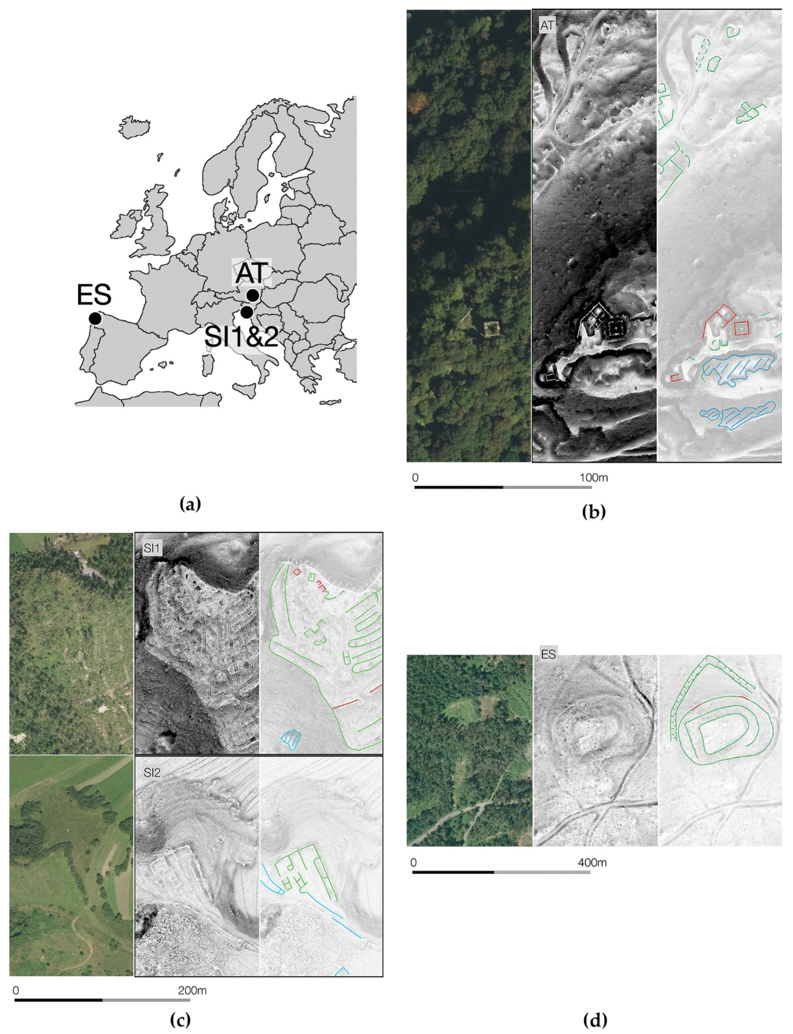
2.1. Test Data

Test data from Austria (AT), Slovenia (SI1), and Spain (ES) were selected based on their archaeological and morphological similarity. Each site features a hilltop settlement (archaeology), buildings (modern), vegetation on steep slopes, and sharp discontinuities. An additional test site (SI2) was chosen as an example of relentlessly dense low vegetation. Each test site is 1000 × 1000 m (Appendix A), but only the most relevant windows are shown in illustrations (Figure 3). All data sets are stemming from nationwide data acquisitions and are publicly available. The key difference between them is the average density: AT 18.79 pts/m², SI 12.43 pts/m², and ES 1.83 pts/m². Test data is described in more detail elsewhere [20].

2.2. Automatic Ground Point and Object-Type Classification

In our approach, automatic ground point and object-type classification are intertwined and presented together.

Despite great progress in the last two decades (e.g., [36,37,38,39,40,41,42,43,44]), ground point classification–also known as semantic labeling of the dataset–remains the most challenging part of airborne LiDAR data processing [19,45]. Recently, the performance of nine automatic filters implemented in free or low-cost off-the-shelf software was qualitatively and quantitatively compared [20] (Figure 4). It was found that no filter is best in all conditions, but the Progressive Triangulated Irregular Network filter (implemented in commercial LAStools: lasground_new by Rapidlasso GmbH, Gilching, Germany) and the hybrid filter from Blue Marble Geographic (implemented in commercial GlobalMapper by Blue Marble Geographics, Hallowell, ME, USA) are consistently at the top in all categories, followed by slope-based filtering (implemented in open source WhiteboxTools: LidarGroundPointFilter by Whitebox Geospatial Inc., Guelph, Canada). The full results of the qualitative comparison are summarized in Figure 5. Two noteworthy conclusions emerge from the study. First, the two commercial filters consistently outperform open access filters. Second, filters based on an older generation of algorithms consistently outperform the newer ones.

Building on these results, an archaeology-specific pipeline for point cloud processing can be proposed. The best practice approach is to first assess the data quality, for example, using the DFM confidence map tool [32]. Then, the archaeological and morphological characteristics of the area are evaluated against the performance of different filters (Figure 5). Based on this, the most appropriate filter and filter settings are selected ([20]: Appendix A). However, such an approach is best suited for small areas, for example, an area of a single site and its surroundings. If larger areas with different conditions need to be processed, there are two possible solutions: averaging or segmentation.

In archaeological practice, the averaging approach–using default settings that are not optimized for any specific conditions, but perform satisfactorily in all conditions [46]—is most commonly used. However, the default settings are usually optimized to eliminate the anomalies that are most unsettling for general-purpose DTM. This, however, is not desirable in archaeology-specific processing. The reason is that, morphologically speaking, archaeological features are anomalies, i.e., sporadically occurring atypical features of the terrain [32]. In terms of processing, archaeological features are therefore often the very anomalies that the default settings were designed to remove, whereas archaeology-specific processing favors feature retention over anomaly removal (as long as the size of the anomalies is significantly smaller and/or significantly different from archaeological features). At the very least, therefore, archaeology-specific average settings must be used [20].

In the segmentation approach, the area is partitioned so that the most suitable filter or filter settings are applied to each segment. For example, in a case study addressing bathymetric green laser LiDAR data, the area was partitioned according to the vegetation point density [19]. However, for red laser topographic airborne LiDAR data, there is no disadvantage in processing the entire dataset with settings for dense vegetation [20]. In a similar vein, within a single project, data quality and expected archaeological features can usually be considered constant. The remaining differentiating factor is geomorphology.

The effects of geomorphology on automatic ground point and object type classification can be demonstrated by AT test data, which includes both plains and sharp discontinuities such as sharp ridges and cliffs. The latter in particular are among the most difficult situations to process [20,47] (Figure 5), as it is difficult to distinguish between vegetation and ground on a forested sharp ridge. Settings can be optimized either for vegetation removal or ridge retention. However, this either/or decision could be circumvented with segmentation. First, a coarse DTM would be created, analyzed, and segmented into areas with or without sharp ridges. Then, the segments without sharp ridges would be processed with settings optimized for vegetation removal, and the segments with sharp ridges would be processed with settings optimized for ridge retention. Finally, the segments would be merged in the final point cloud (Figure 6). However, this is difficult to do with the existing off-the-shelf tools due to the so-called edge effect (points on the edge cannot be processed optimally) and the problems with processing non-rectangular datasets. The workaround would be to process the entire dataset twice, once for each setting, and then segment it. This would multiply the processing time by the number of segments. More importantly, such an approach is too complex to implement in a robust, unified pipeline and it can produce severe negative results under some fringe conditions.

Morphologically similar is the problem between building detection accuracy and archaeological feature retention. For example, several filters use the size of the initial search window, where a large search window negatively affects the classification of potential archaeological features as ground, while a small window classifies large buildings as ground [20]. In this case, however, either/or choice can be avoided by sequential processing. Unlike ridges, which are part of the ground (classified as class 2 according to the classification scheme of the American Society for Photogrammetry and Remote Sensing [48]—hereafter ASPRS class), buildings are classified separately (ASPRS class 6). Therefore, ground points can first be classified in a manner optimal for building classification, and then buildings are classified. Second, the classification of ground points is repeated with settings optimized to retain archaeological features, but already classified buildings are withheld. The result is an optimal classification of both ground and building points. Although this doubles the processing time, the solution is straightforward to implement with existing tools and there are no (known) negative effects under any conditions.

Two further point cloud processing issues can be addressed here. First, all filters tested in [20] perform the ground classification by default only for the last return points. The intention is to minimize T2 error (false positive classification) at the expense of higher T1 error (false negative classification) [47]. In other words, less noise at the expense of lower ground point density. If the data density is sufficient, this is a desirable result. However, if the data density is low, this can lead to poorer recognition of archaeological features. Correct classification of non-last-return ground points can be achieved by a relatively simple additional processing step. After the initial classification of last-return ground points, all non-classified points within a certain Z-axis distance to the last-return ground points, for example ± 0.2 m, are also classified as ground.

Second, vegetation points are addressed. They are only occasionally directly relevant to archaeological interpretation, e.g., [49], but low vegetation density can be used both for planning ground surveys [5] and as one of the proxies for the accuracy of the final model [32]. Regarding the latter, the actual height of relevant vegetation depends on the specific vegetation structure [50], but in the context of a multipurpose pipeline, the widely accepted ASPRS standard [48] makes the most sense (low vegetation between 0.5 and 2.0 m, medium vegetation between 2.0 and 5.0 m, and high vegetation above 5.0 m).

In summation, despite the obvious shortcomings and trade-offs, the averaging approach is still currently the best option for point cloud processing to be incorporated into a general-purpose rigid processing pipeline. We have proposed some improvements by introducing sequential processing. A segmentation approach would probably further improve the results, but the problems of instability and unpredictability need to be solved first.

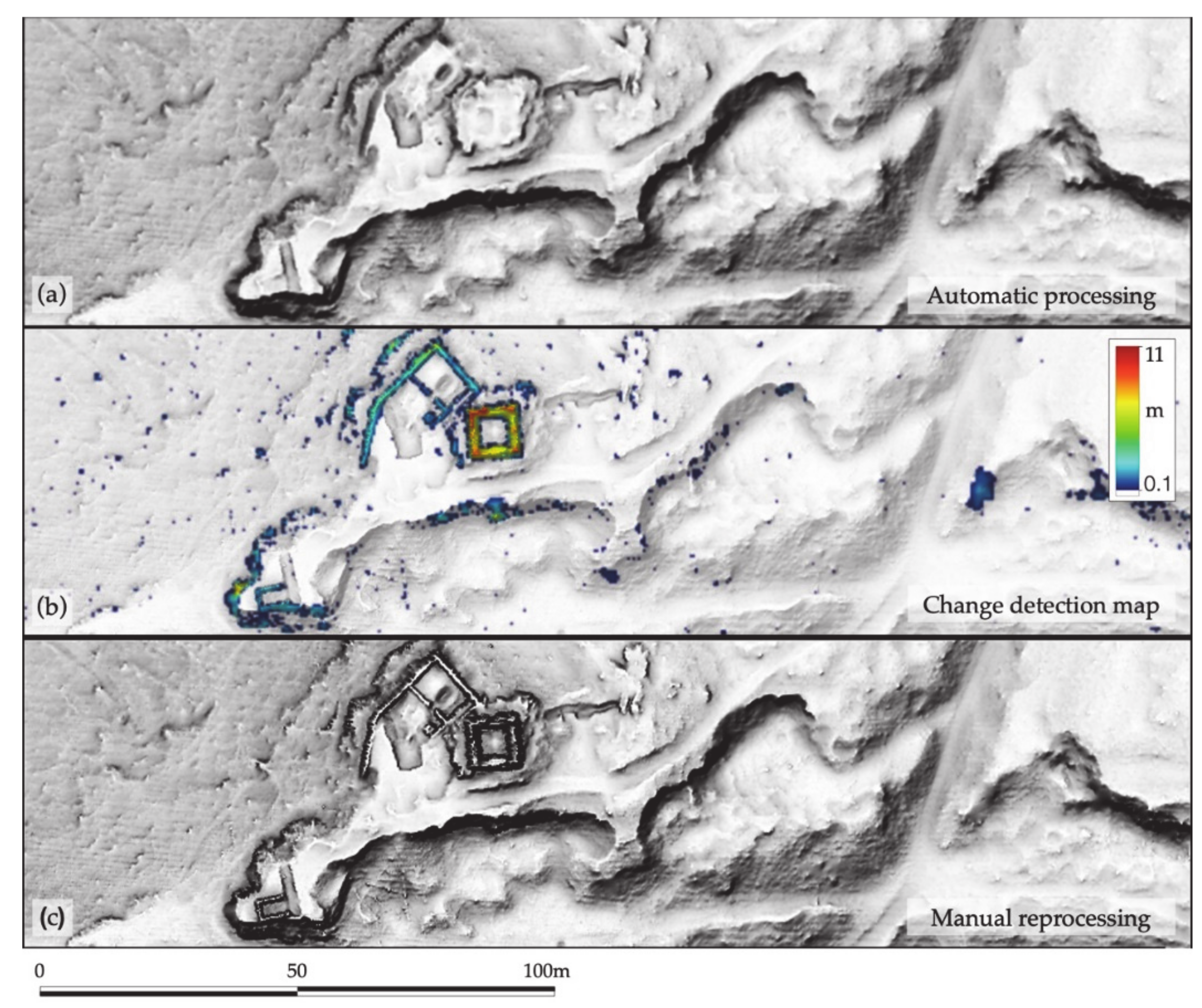
2.3. Manual Reclassification

Manual reclassification has received relatively little attention in archaeology. However, total errors in archaeology-specific automatic ground point classification can range from 0.1% to 63% [20]. If the total error is considered too high, additional manual reclassification of the point cloud is required. Archaeological features near ground discontinuities and standing archaeological features are particularly prone to error, both exacerbated by dense vegetation. A typical context where manual reclassification is required is a castle ruin standing in woodland on the top of a cliff (Figure 7). A typical context where automatic classification is sufficient is embedded features in an undulating grassland (Figure 3c). Regardless of the severity of the total error, manual reclassification is typically limited to areas of high archaeological significance [18,35].

Manual reclassification is performed by viewing the points in the profile and reclassifying those that are incorrectly assigned. The process is guided by the operator’s experience and knowledge of the specific geomorphology, vegetation structure, and typical archaeological features. Multitemporal aerial photographs are a welcome aid, as is the fact that the operator is personally familiar with the area. To this end, on rare occasions, a field survey is conducted to assist in manual reclassification for selected small areas. One such example was carried out on a medium-sized site of a Roman military camp and took one day of fieldwork by a team of two people [35]. In comparison, mapping the same site with a laser total station and a dGPS [51] took a team of three people almost a week.

Manual reclassification thus consists of a series of subjective “microdecisions” by the operator (for example, when a single point in the point cloud is considered individually). If the result is to be admissible as scientific data, this process must be documented. There is currently no standard way to document metadata for each point in the point cloud. One possibility would be to assign manually reclassified ground points to one of the user-definable classes, for example, class 64. This would be accurate, but impractical. Therefore, we proposed a change detection map. The change detection map takes the form of a Z-coded absolute difference calculated by subtracting the DFM before and the DFM after manual reclassification. Such a change detection map is informative, it adequately documents the location (x, y) and magnitude (z) of the effect that the manual reclassification has on the final DFM, and it is straightforward to produce with map algebra [5] (Figure 7).

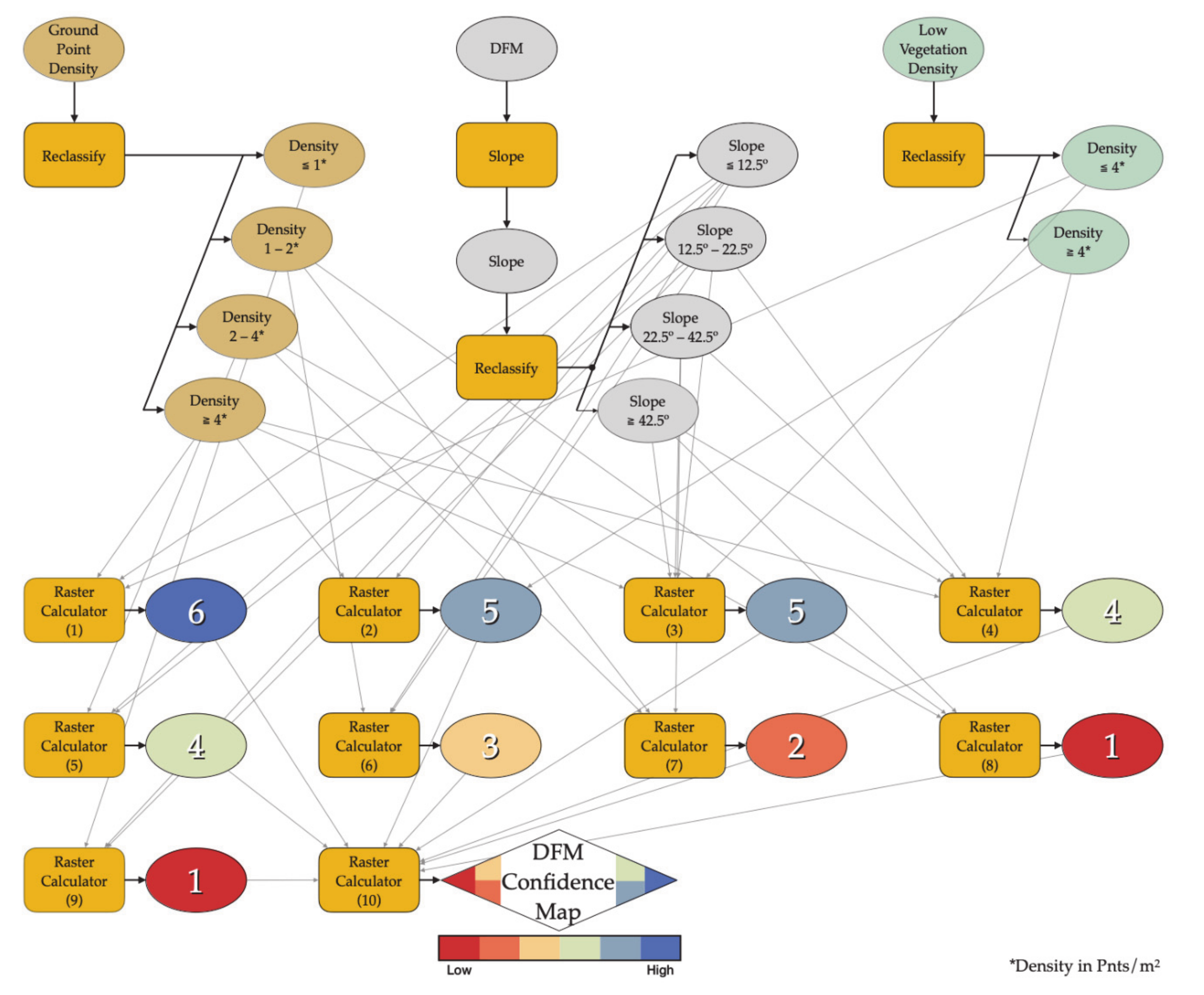
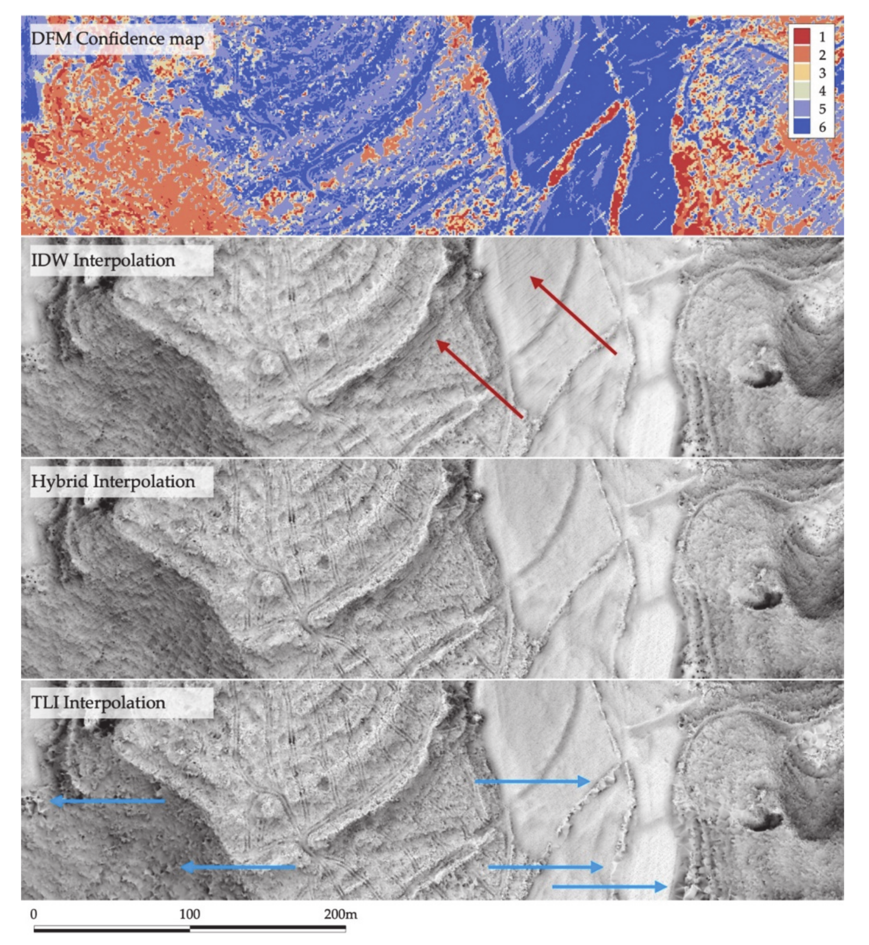
2.4. DFM Interpolation

Interpolation is also referred to as rasterization or gridding and has a direct impact on the accuracy and visual quality of the final DEM. It is a process of fitting a surface to point elevation data by effectively draping a grid of defined cell size over the point data. This means that the points are derived from the original data and do not consist of the actual data points [52,53,54]. Despite numerous studies, interpolation remains a challenge. A recent review concluded that existing methods for generating DEM from airborne LiDAR data have difficulties when used either in sharply changing terrain, or in areas with dense non-ground features, or complex landscapes [55]. The multitude of accuracy assessment analyses shows that choosing the appropriate interpolator is problematic, as each method has its advantages and disadvantages [56]. In practice, Kriging-based methods are considered capable of producing more accurate DEMs, but are computationally intensive. Inverse distance weighting (IDW), nearest neighbor, and triangulation with linear interpolation (TLI) are simple and fast methods to generate relatively accurate DEMs, but their performances decrease and become sensitive to topographic variations as the spatial resolution of DEM increases. Spline appears to offer a trade-off between computation time and accuracy at high resolutions but becomes less reliable at low resolutions [57].

In contrast to the extensive literature on DEM interpolation, interpolation of archaeology-specific DFM has until recently been briefly considered in only a handful of studies with conflicting results: TLI [58], Kriging [35,59], spline interpolator [60], and nearest neighbor [61] were all declared as the most suitable interpolator. A recent study was therefore dedicated to finding the most suitable interpolator for archaeology-specific processing of airborne LiDAR data. Six of the most commonly used interpolators were reviewed and their archaeology-specific precision was tested at four test sites. In addition to visual precision, accessibility and computational cost were also considered. The study found that although Kriging gives the best results, IDW is currently the most suitable archaeology-specific interpolator, mainly because of its accessibility [31].

This is not to say that IDW is without flaws, as the aforementioned study shows. In severely undersampled areas (where the density of measurement points is much lower than the density of grid cells), it introduced a relatively dense pattern of negative interpolation artifacts, i.e., errors in the form of exaggerated negative values. In moderately undersampled areas it was most pleasing to the eye as there were no positive artifacts, but there were very small negative artefacts and a slight scaling effect (artefacts in the form of fish scales) on slopes. This effect was not too visually disturbing, but it may lead an inexperienced interpreter (or an experienced interpreter without sufficient metadata) to erroneously conclude that the slope was terraced. In slightly undersampled areas IDW tends to show data noise resulting from the pattern of measurement points that could be mistaken for geologic features or the like. In areas where the density of measurement points is similar to or higher than the density of grid cells, IDW exhibited some over-smoothing, which is not optimal for archaeology-specific interpolation.

In the same study, the ephemeral nature of the results was also mentioned. Ordinary Kriging is a superior interpolator, but it lacks accessibility in most relevant software packages. With improved accessibility, it could instantly become the most suitable archaeology-specific interpolator. The study also highlighted the potential of a hybrid interpolator that would combine IDW and TLI. IDW and TLI both excel in high accessibility and low computational cost; TLI is the best interpolator for oversampled areas and IDW’s comparative strength is in undersampled areas [31].

In the past, the key missing component for such a hybrid interpolator was a suitable segmentation method that allows the partition of the data into areas best suited for each interpolator [56]. Recently, this has been solved by using classification and regression tree analysis to derive the DTM uncertainty prediction map [62,63]. We modified this method to create an archaeology-specific DFM confidence map that assigns a confidence level between one and six to each grid cell. The quality of the DFM is thus quantified at the cell level [32] (Figure 8). When the interpolators were assessed against the DFM confidence map, TLI is the best interpolator for areas with confidence map levels five and six and performs well in levels three and four. IDW is the best among widely accessible interpolators in areas with confidence map levels one and two and performs well in levels three and four [31].

Once the segmentation was resolved the only remaining problem for implementing a hybrid interpolator was that TLI and IDW interpolators, by definition, produce a slightly different grid model. If they were simply merged by the map algebra, artifacts in the form of steps would be produced in the contact zones between the two interpolators. This is inherent in any hybrid interpolator and cannot be completely avoided, but it can be mitigated.

We undertook three separate mitigating measures. First, contact zones can be reduced by defragmentation. Namely, under certain landscape and/or data acquisition conditions—such as a test site SI1 (Figure 9)—the confidence map values are highly fragmented. In such conditions, the contact area grows exponentially and at the same time, the positive effects of hybrid interpolation are diminished. This can be alleviated by setting a minimum area size of each interpolation patch well above the single-cell size.

Experimentally, the zonal statistic with the neighborhood size 11 cells (which ensures that there are no patches smaller than 6 cells) was chosen as the most efficient. Second, the deviations between the two interpolators are not uniform. TLI and IDW are most similar in confidence zones three and four, and thus the deviations between the two are smallest there (Figure 10). Therefore, the contact zone is smoothest when it lies between confidence levels three and four. Third, measures can be taken to smooth the remaining step-artifact. We introduced a buffer in the contact zone within which the elevation is the mean of the TLI and IDW. We experimented with one-, three-, and five-cell buffers with weighted averages. In most cases, the results were very similar, but in rare extreme examples, wider buffers led to even larger artifacts. Therefore, we decided to use the single-cell buffer.

After initial testing, we found that certain donut-shaped artifacts occurred where areas with DFM confidence map level one were directly adjacent to level four or higher (Figure 11). To counteract this, the contact zone was “grown”, i.e., moved further into the level four areas. Experimentally, the 3-cell shift proved to be sufficient.

Thus, all requirements for implementing hybrid interpolation have been met (Figure 9). The procedure is as follows. First, the entire point cloud is interpolated using both interpolators. Then, the area is segmented by reclassifying the DFM confidence map into “red” (levels one to three for IDW) and “blue” segments (levels four to six for TLI). Then, defragmentation and a three-cell shift are performed. Afterward, a one-cell wide contact zone buffer is defined, within which the mean elevation value of the two interpolators is used. The final step is to merge “red”, “blue”, and buffer segments using map algebra (Figure 12).

2.5. Enhanced Visualization

Enhanced visualization is needed to take advantage of the archaeological information embedded in DFM. Hillshading (also known as relief shading or shaded relief) was one of the earliest [64] and remains the most widely used DEM visualization technique because it is simple to compute and unambiguous to interpret [33]. However, on its own, it is insufficient for archaeology-specific workflows and several enhanced DFM visualization techniques have been proposed. Some have reused existing DEM -derivatives for visualization (for example, sky view factor [65], openness [66], multiscale topographic position [67]), while others have been developed specifically for archaeology (for example principal component analysis [68], local relief model [69], solar insolation models [70]; enhanced multi-scale topographic position [71]. A representative review discussed 11 techniques in detail [33], although the list is even more extensive. Several comparative studies emphasized that no single technique reveals all archaeological details in a landscape and that multiple techniques should be used simultaneously [70,72,73].

Several techniques are in use in archaeological practice (

Table 2. Qualitative assessment (based on the subjective experience of the authors) of visualizations commonly used in archaeology-specific workflows (compare to [33]). Table heading, archaeological features: e.—embedded; p. e.—partially embedded; s. f.—standing features; s. o.—standing objects (see Figure 2). Table body: 1—poor; 2—medium; 3—good; Y—yes; N—no; W—white (0% black); B—black (100% black); N—neutral, no saturation.

Visualization		Archaeological Features				Relief	Isotropic	Saturation
		e.	p. e.	s. f.	s. o.
HSD	Hillshading	1	1	2	3	2	N	B/W
SVF	Sky view factor	1	2	3	3	3	Y	N
OPP	Opennes (positive)	1	3	3	3	1	Y	B
SIL	Sky illumination	1	1	2	3	3	Y	W
SLP	Slope	2	2	2	3	3	Y	W
LRM	Local relief model	3	2	2	2	2	Y	N
LDO	Local dominance	3	2	2	2	2	Y	N
DME	Difference f/mean elev.	3	2	2	2	2	Y	N
VAT	Vis. f/arch. topography	2	3	3	3	3	Y	N
MTP	Multiscale topo. position	3	1	2	2	1–3 1	Y	N/A
EMS	Enhanced multiscale topographic position	3	3	2	3	1–3 1	Y	N/A

¹ Depending on the training of the operator for this specific visualization technique.

). Viewed through the narrow perspective of visualizing archaeological features and their context, the listed techniques differ in several characteristics. First, anisotropic visualizations (Table 2: HSD) suffer from local saturation, making isotropic solutions superior. Second, a saturation of the image at the black or white end of the spectrum results in loss of detail. Third, different visualizations are differently informative for each morphological type of archaeological feature: embedded features are best visualized with detrending techniques that average the local environment (Table 2: LRM, LDO, DME, MST) and standing features with those techniques that focus the feature (Table 2: SVF, OPP). Among the latter, the sky view factor splits the contrast between the archaeological feature and the relief, while the openness allots it all to the feature.

Despite the undisputed need for the concurrent use of multiple visualizations, there is a need for a single “best” visualization for dissemination, fieldwork, and as an input to machine learning. A recent development in this area in the field of archaeological LiDAR is image fusion, a well-known technique in remote sensing that creates in which a meaningful image combination that preserves the positive characteristics of each input image [71,74,75,76,77,78]. However, applying image fusion to DFM visualizations can further exacerbate the shortcomings typical of complex visualizations: as the complexity grows, it becomes increasingly difficult to interpret the image without specialized training. An example of such a complex image fusion visualization technique is the enhanced multi-scale topographic position [71]. It adopts the color scheme of multiscale topographic position, which requires a key–and thus special training–to interpret (for example, the color blue occurs when a site has highly deviated at the local scale but averagely positioned at the meso- and broad scales [79]). To avoid this, some techniques are specifically designed to be intuitive and straightforward to interpret. An example of this is the visualization for archaeological topography [74].

The above refers to 2D (also known as 2.5D) terrain representations since the 2D GIS environment forms the basis for most interpretive mapping of airborne LiDAR data. Perhaps one of the greatest advantages of 2D is that no parts of the dataset are obscured at any time. Some studies also indicate that 2D visualizations are more comprehensible, accurate, and efficient to interpret than 3D representations in tasks involving spatial memory, spatial identification, and precision [74]. However, when used properly the 3D output additionally allows to extract accurate metric information about the archaeology under study that is not possible with just 2.5D, but there is still a serious lack of tools that allow for easy interaction with these models in a metrical and coordinate system-aware environment [80,81]. However, with the recent development of software and hardware, working side by side in 2D and 3D is becoming increasingly inviting and will undoubtedly eventually be fully integrated into archaeology-specific workflows.

In summary, the archaeology-specific workflow is currently still based on a 2D GIS environment using multiple complementary DFM visualization techniques. In our subjective opinion, visualization for archaeological topography is currently the best overall solution for human-based interpretative mapping (Table 2) and a recent objective analysis proposed enhanced multiscale topographic index as the best solution for machine-learning-supported interpretative mapping [71]. Given the strengths and weaknesses of commonly used visualization techniques (Table 2), we advocate as a minimum the concurrent use of sky view factor, opennes, the difference from mean elevation (LRM, LDO, and DME are almost indistinguishable visually, but DME is by far the least computationally intensive and it outputs Z-axis values in realistic map units; see [79]), and visualization for archaeological topography.

2.6. Pipeline and Toolbox

Above, each step of the workflow from point cloud to DFM visualization (Table 1: 2.1 to 2.5) was discussed separately. This paper aims to present a unified pipeline that executes all steps. As mentioned earlier, a rigid pipeline with static settings will inevitably lead to trade-offs, such as between vegetation removal and retention of archaeological features. The future lies in adaptive solutions that will be based on segmentation. However, as a first viable solution, we present an archaeology-specific rigid pipeline optimized for low- to medium-density data, typically obtained from national repositories of general-purpose datasets.

We implemented a mixture of averaging and segmentation techniques (Figure 13). The point cloud processing is based on averaging enhanced by sequential processing. First, the buildings are classified with settings optimized for building detection. Then, the entire point cloud without buildings is reprocessed with settings optimized for ground point detection, which favors the retention of archaeological features over vegetation removal. An additional step, targeting low-density data, is to classify all unclassified points that are within ± 0.2 m of ground points as ground points. Vegetation points are classified according to the ASPR scheme. However, due to software limitations and streamlining of the pipeline, medium and high vegetation are combined into class 5. The classified point cloud is used to derive the ground point density map, the low vegetation density map, and to interpolate the DFM. The latter is based on the segmentation approach. The DFM is used to derive the DFM confidence map and four DFM visualizations (sky view factor, opennes, difference from mean elevation, visualization for archaeological topography).

To facilitate the computation, we have developed an open-source tool in the form of a QGIS plug-in. It is called One-step-processing or One for short and it comes as a part of the Open LiDAR toolbox [82]. It is important to note that One only calls individual tools that must already be installed in QGIS. In other words, One provides an envelope for six different GIS software packages (Figure 13): QGIS native algorithms [82], GRASS GIS [83], GDAL library [84], LAStools [85], Whitebox tools [86], and Relief Visualization Toolbox [74]. The first three are included with most QGIS installers, and the last three are QGIS plug-ins that must be installed manually. This also means that the original copyright licenses of the listed tools apply (LAStools is a hybrid licensed software, the rest are open source).

In the first step of creating the One, we built the pipeline in the graphical model designer of QGIS (Figure 13). In the second step, the pipeline was implemented in the Python programming language to create a QGIS plug-in. The plug-in was tested in the latest long-term release of QGIS 3.16.x on Windows 10, macOS Big Sur, and Linux Ubuntu 20.04.

3. Results

In this section, the pipeline and toolbox presented above were tested on data from four test sites (Figure 3). Each step of the processing pipeline was tested separately and compared to the results of the conventional processing method previously developed by the authors [35] (

Table 3. Paradata for conventional point cloud processing and derivation of products to which the proposed pipeline has been compared (paradata structure after [5]).

Step	Type	Paradata
(2.1) Automatic ground point classification	Software	LAStools 1.4 Rapidlasso GmbH
	Filter	lasground_new
	Settings	st: 5; g:/; off: 0.05; s+: 1.0; s−: 1.0; b: no; terrain type: wilderness; pre-processing: ultra fine
(2.2) Object-type classification	Software	LAStools 1.4 Rapidlasso GmbH
	Filter	lasheight
	Settings	classify between: 0.5 and 2 as 3; classify between: 2 and 5 as 4; classify above: 5 as 5
	Software	LAStools 1.4 Rapidlasso GmbH
	Filter	lasclassify
	Settings	building planarity: 0.1; forest ruggedness: 0.4; ground offset: 1.8
(2.3) Manual reclassification	Yes	See ŠtuLoz2020
(2.4) DFM interpolation	Software	Surfer 19.2.x, Golden Software
	Filter	Kriging
	Settings	Kriging type: point; Drift: none; No. sectors: 4; Max. all sectors: 64; Max. each sector: 16; Min. all sectors: 8; Radius 1: 20; Radius 2: 20; cell size: 0.25 m.
(2.5) Enhanced visualization	Software	RVT 2.2.1, ZRC SAZU
	Filter	Sky view factor
	Settings	No. search directions: 32; Search radius: 10; Remove noise: no; scale: linear stretch between 0.6 and 1.0.

). For example, when point cloud classification is discussed, the point cloud is processed according to the proposed pipeline and interpolation according to Table 3, and vice versa, when interpolation is discussed, the point cloud is processed according to Table 3. In this process, 273 files were generated.

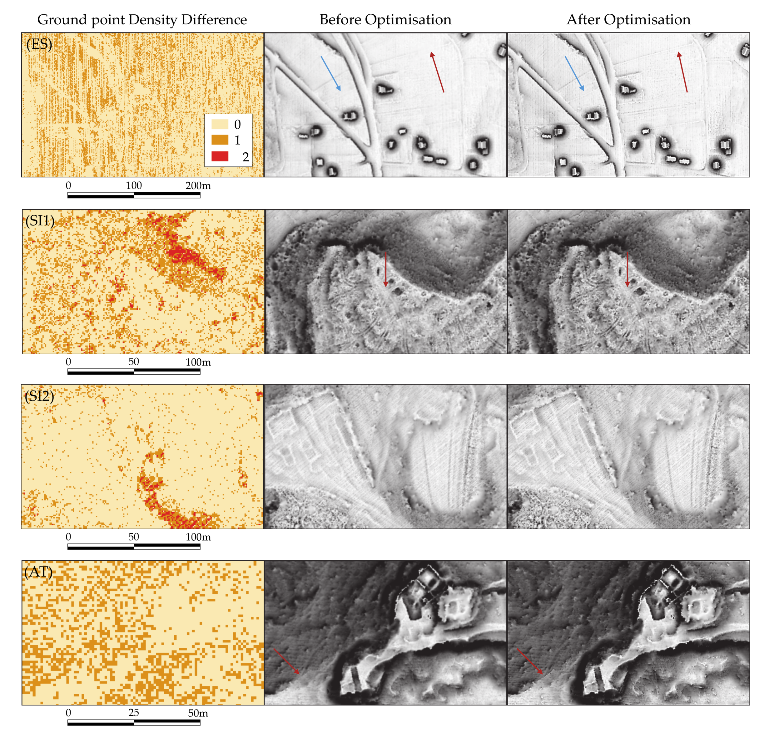
3.1. Automatic Ground Point and Object-Type Classification

The proposed pipeline introduces several additional steps compared to a traditional approach. The first additional step optimizes the correct classification of buildings. This step specifically targets suburban contexts where archaeological features are adjacent to, for example, large industrial buildings (Appendix A: SI2). Misclassification of buildings by archaeology-optimized processing has limited impact on the DFM but produces incorrect DTMs. On the other hand, building-optimized processing leads to significant deficiencies, for example, in sharp terrain. The proposed sequential processing mitigates all issues as it combines the qualities of each step (Figure 14). Thus, if the only goal of point cloud classification is to produce DFM for visual inspection, the benefits of the proposed approach are limited to a more accurate building representation. However, the real advantages lie in the ability to generate DTMs for further analysis and in the classification of certain types of archaeological standing objects as buildings. The latter is particularly useful, for example, in a situation where standing objects are ubiquitous and modern buildings are absent, e.g., [87,88,89,90,91]. In such morphological contexts, the proposed pipeline (with possible tweaks to the settings) can be used for automatic feature detection at the point cloud level, which has many advantages.

The final step in ground point classification is the detection of non-last-return ground points. As mentioned earlier, in general-purpose processing this step is largely avoided because it introduces noise, i.e., it reduces false-negative errors at the expense of increasing false positive errors. The key to implementing this feature is therefore to balance noise and feature detection. As expected, the actual gain in point density is greatest in an open landscape without vegetation (that is higher than 0.5 m above ground), where non-last-return pulses are reflected from the ground. As for archaeological feature detection in our test areas, the gains were moderate (Figure 15). The difference was most pronounced in the open landscape of the low-density test site ES, where additional field boundaries could be detected. There were very limited benefits for test site SI1 and no benefits for SI2. Perhaps the greatest improvement was observed on the steep slope of the high-density data from the test site AT. This was encouraging since the procedure was largely developed with steep slopes in mind. Another very positive result was that noise increase was undetectable (ES, SI2, and AT) or negligible (SI1). Thus, this processing step is moderately beneficial for the pipeline with negligible negative effects.

3.2. DFM Interpolation

As mentioned earlier, DFM interpolation has been largely overlooked in the relevant archaeological literature. One of the reasons for this is that its effects are visually less profound than those of point cloud processing or the use of appropriate visualization techniques. Nevertheless, the differences between, for example, ordinary Kriging and nearest-neighbor interpolation can mean the difference between detection and non-detection of an archaeological feature [31]. The differences between the interpolators are particularly apparent for low-density data, such as the test site ES (Figure 16). Interpolation is also the area where, as is often the case [31,92], the quality of the results is software specific. Pertaining to the matter at hand is the fact that open source solutions for Kriging and IDW fall short of the best commercial solutions [31]. Consequently, interpolation is the only part of the proposed pipeline where the quality of the final product must be compromised to make the functionality available through the QGIS platform. Namely, the hybrid interpolation results are significantly better when the input IDW is computed using the commercial Golden Software Surfer (Figure 16d) than using the Whitebox tools (Figure 16c), which represent the best available open-source solution [31].

Regardless, the main drawback of the proposed hybrid interpolation is the interpolation artifacts in the contact zones, which can resemble potential standing features (Figure 11). The measures introduced to minimize this effect were 100% successful in our test data, but this may not be the case for all datasets. Therefore, anyone using this interpolator for interpretative mapping of archaeological features must be trained to recognize these noise artifacts. It must also be emphasized that hybrid interpolation is primarily intended for use in creating DFMs for visual analysis. Its use for creating DTMs, for example, for hydrological analysis, has not yet been tested. An avenue of possible further development is to use the same approach for combining ordinary Kriging and TLI interpolations. Somewhat surprisingly, the current version of the hybrid algorithm has produced very satisfactory results without any changes to the mechanics of merging (Figure 16e).

Overall, the hybrid interpolation performed surprisingly well on our test data. No introduced artifacts were detected and the strength of the interpolation came through clearly. The results obtained by interpolating TLI and IDW in Golden Software Surfer are a very close approximation to the perfect archaeology-specific interpolation. The results obtained by interpolating TLI and IDW in the Whitebox tools used by our tool are noticeably inferior in the IDW parts, but overall the result is still superior to any free-to-use solution known to us [31].

3.3. Enhanced Visualization

Enhanced visualization is not an area of innovation in the proposed pipeline. We provide four DFM visualizations that are the most useful and versatile in our own subjective experience (Figure 17). They have been selected to cover all aspects of intended use for archaeology-specific interpretative mapping (

Table 4. DFM visualization techniques included in the pipeline and their primary use in interpretative mapping of archaeological features.

Visualization Technique		Primary Use
SVF	Sky view factor	Standing objects, relief
OPP	Opennes (positive)	Standing f., partially embedded f.; steep slopes
DME	Difference f/mean elev.	Embedded features; flats
VAT	Vis. f/arch. topography	Overall performance; dissemination

). However, users are able and indeed encouraged, to create additional visualizations using the DFM generated by the pipeline.

3.4. Documenting the Process (Metadata and Paradata)

Documentation of archaeology-specific workflow for processing airborne lidar data was not a topic in the relevant literature until recently, when the first step towards standardization was proposed [5]. In this paper, we adhere to the proposed schema for documenting the paradata. Specifically, the paradata are documented for the proposed pipeline implemented by the provided tool One (

Table 5. Paradata for the proposed pipeline as implemented with Open LiDAR Toolbox tool One (paradata structure after [5]). Since the One only calls different tools, the original software packages are listed.

Step	Type	Paradata
(2.1) Automatic ground point classification	Software	LAStools 1.4 Rapidlasso GmbH
	Filter	lasground_new
	Settings	s St: 5; g:/; Off: 0.05; s+: 1.0; s−: 1.0; b: no; Terrain type: city; Pre-processing: fine
	Software	LAStools 1.4 Rapidlasso GmbH
	Filter	lasground_new
	Settings	St: 5; g:/; Off: 0.05; s+: 1.0; s−: 1.0; b: no; Terrain type: wilderness; Pre-processing: ultra fine
(2.2) Object-type classification	Software	LAStools 1.4 Rapidlasso GmbH
	Filter	lasheight
	Settings	classify between: −0.2 and 0.2 as 2; classify between: 0.5 and 2 as 3; Classify above: 2 as 5
	Software	LAStools 1.4 Rapidlasso GmbH
	Filter	lasclassify
	Settings	Building planarity: 0.1; Forest ruggedness: 0.4; Ground offset: 1.8
(2.3) Manual reclassification	Yes	See Figure 7
(2.4) DFM interpolation	Software	Open LiDAR Toolbox
	Filter	Hybrid
	Settings	Cell size: 0.5 m
(2.5) Enhanced visualization	Software	Relief Visualization Toolbox 0.6.x (QGIS plug-in)
	Filter	Sky view factor
	Settings	No. search directions: 32; Search radius: 10; Remove noise: no; Scale: linear stretch between 0.6 and 1.0.
	Software	Relief Visualization Toolbox 0.6.x (QGIS plug-in)
	Filter	Opennes–positive
	Settings	No. search directions: 32; Search radius: 10; Remove noise: no; Scale: linear stretch between 0.6 and 1.0.
	Software	Relief Visualization Toolbox 0.6.x (QGIS plug-in)
	Filter	Blender
	Settings	Combination: Archaeological (VAT); Terrain type: general
	Software	Whitebox tools 1.2 (QGIS plug-in)
	Filter	DiffFromMeanElev
	Settings	Filter X dimension: 10; Filter Y dimension: 10

). However, whenever the One is used in a scientific process, we suggest that a simple bibliographic reference to the pipeline presented in this paper will suffice in lieu of the paradata.

In addition to the above paradata, the pipeline produces three outputs that are aimed at visualizing the metadata of the LiDAR source data.

Ground point density and low vegetation density, both calculated within a 1 m radius and for a grid cell size of 1 m, visualize point cloud properties. Ground point density is the most common tool for visualizing the quality of airborne LiDAR data. The 1 m setting is archaeology specific as this metadata visualization is to be used at the feature level. Low vegetation point density is a less common proxy for data quality [50]. It was included primarily to be used for planning ground assessment expeditions. For example, areas with a high density of low vegetation should be targeted during the low vegetation season (for example, Winter in temperate zones), while the same areas may not be accessible during the height of the growing season (for example, Summer in temperate zones) [5].

The DFM confidence map provides metadata that is a necessary part of the workflow documentation, helps in the process of interpretative mapping, and also enables the determination of the appropriate DFM resolution. While ground point density is an indirect proxy, the DFM confidence map is a direct measure of the quality of the DFM used for interpretative mapping. We propose that at the very least, the DFM confidence map should become a standard part of reporting the airborne LiDAR data quality, both at a dataset and feature levels [32].

3.5. Open LiDAR Toolbox

As mentioned earlier, we have developed a software tool–One-step-processing or One for short–to complement the proposed pipeline, which is a part of our Open LiDAR Toolbox (see Supplementary Materials). The One provides a one-click implementation of the entire pipeline. Selected parts of the pipeline will eventually be available as separate tools to enable different use case scenarios. The tool is provided as a QGIS plug-in and, for users who need more control over settings, as a QGIS model [93]. We chose the QGIS platform for its accessibility (open-source, multi-platform) and functionality. The latter is powered by the fact that in recent years most community-driven GIS software projects and many commercial ones have also been made available as QGIS plug-ins. Our focus was on open source tools, but we include the commercial LAStools because they are unique in their functionality [20] and are free-to-use (under certain conditions and with certain drawbacks [85]).

The One tool leverages the power of the QGIS platform to automate the pipeline, which consists of 17 algorithms from five software packages or libraries and includes 62 processing steps (Figure 8, Figure 12, and Figure 13). On a modern notebook, our test data runs for 192 (ES, 1.8 × 10⁶ points, 1 × 10⁶ grid cells), 408 (SI1 and SI2, 12.5 × 10⁶ points, 5 × 10⁶ grid cells), and 604 s (AT, 18.8 × 10⁶ points, 16 × 10⁶ grid cells). If the same pipeline is executed manually and the user spends only 30 s to set up each of the 62 steps, the whole process is between 4 and 10 times longer. In addition, the QGIS platform includes powerful batching tools that allow the One to be applied to mosaicked datasets (for optimal results the data must be mosaicked with overlap) of unlimited size. Another important advantage of the QGIS platform is that it runs on most major OS platforms and modest hardware configurations.

As for the results, it is important to emphasize the difference between the pipeline (which can be executed on different software platforms) and the tool (which is limited to the QGIS platform). The only processing step where the solutions available in QGIS lag behind the industry leader is interpolation. This is somewhat surprising since interpolation is a mature field in GIS science and the same interpolators have been in use for decades. However, most of the open-source tools have not been updated for LiDAR data and cannot be used in a production environment [31]. To compensate for the shortcomings of QGIS, we developed a hybrid interpolator. However, despite the significant improvements, the results are still underwhelming (Figure 16). We are hopeful that this can be addressed in the future.

4. Discussion

From the outside, processing airborne LiDAR data may seem like a dull and repetitive task that is completely objective. However, this is not the case [5]. But this misconception runs deep in archaeological practice, especially outside the community of LiDAR data specialists [18,19]. In practice, archaeologists all too often depend on external experts to process the airborne LiDAR data from raw data to visualizations, and sometimes even interpretive mapping is outsourced to non-archaeologists, e.g., [91]. The consequence, as we indicated in the introduction, is that derivatives (for example, DTM visualizations) are most often accepted as facts rather than “facts” (sensu Clarke [22]), which is at least partly the consequence of black-boxing the data processing. In this discussion, we want to present our personal and somewhat subjective view on the extension of the dichotomy between facts and “facts” in the particular context of landscape archaeology and airborne lidar data processing. The discussion perhaps strays somewhat from the main topic of the article, but it is necessary to place the processing pipeline in the context of contemporary landscape archaeology.

First, we need to describe the dichotomy between facts and “facts” in a little more detail and look at LiDAR data more closely. Despite the lack of an agreeable set of definitions of data, information, and knowledge, there is a general consensus to use Ackoff’s Data-Information-Knowledge-Wisdom hierarchy [94] as a starting point, e.g., [95]. For the purpose of our discussion this general classification suffices and furthermore, we are following Chen and colleagues [96] in believing that for our purpose we can generalize knowledge to include also wisdom, and any other high-level of understanding, without losing generality. In LiDAR point cloud processing we are dealing with data (i.e., numbers or graphs produced by, for example, sensors and smart meters), information (i.e., data that are processed to be useful, providing answers to ‘who’, ‘what’, ‘where’, and ‘when’ questions), and knowledge (i.e., application of data and information, providing answers to ‘how’ questions). Taking a somewhat simplistic and rigid view, one could say that raw data and point cloud processing is predominantly about data, interpretative mapping is about information, and deep interpretation with possible subsequent steps of archaeological interpretation is predominantly about knowledge production (Figure 18a). However, as is almost invariably the case, archaeological practice is messy and the process is fuzzy and often recursive. If pressed, pure hard data can be identified at the beginning of raw data processing, when sensor data is acquired and transferred to the computer. It is even more difficult to pinpoint “pure knowledge,” if it exists at all. Not to delve too deeply into the philosophy of science, it may be said that knowledge is certainly the predominant aspect of the workflow step called “deep interpretation” [5,27] (Figure 18b).

The key message of the above is that, almost immediately after the raw data is acquired, we are no longer dealing solely with hard data and facts. The data derivatives that archaeologists most often rely on to provide meaningful information are, by definition, amalgams of hard and soft data with injected knowledge. In short, they are “facts”.

Having defined the dichotomy, we can turn to its implications in landscape archaeology. Landscape studies in archaeology rely on the ability to see large tracts of land or urban landscapes at once and to identify and document patterns and relationships in the data [97]. Knowledge, however, is not discovered but constructed, that is, produced through scientific practice [98], which often includes the need for scientists to resort to complex devices [24]. Airborne LiDAR scanning systems are a prime example of such complex assemblages of technologies, e.g., [99]. It has been argued that these instruments are the “interface” between the archaeological landscape and the knowledge-producing landscape archaeologist [100]. Understanding the full impact that this knowledge construction process has on the interpretative and analytical framework of airborne LiDAR data requires introspection in digital archaeology; an approach that consciously seeks to understand the processes behind the tools, techniques, and technologies used in the creation of archaeological knowledge [101]. It is therefore beneficial to consider how digital tools force us to think differently [30]. For example, traditional field-based mapping can provide a deeper insight into the complexity of a site than a digital recording [102].

We argue that airborne LiDAR data processing is an intricate part of the above-mentioned technology that provides the “interface” between the landscape and the archaeologist. In this particular example, data processing accounts for more than 90 percent of the “interface”, if the work hours spent and the involvement of archaeologists (Table 1) are taken as indicators. Therefore, the creation of knowledge about the archaeological landscape, i.e., archaeological interpretation, cannot be separated from data processing. The negative effects of such a separation [5,17,18,19,20,27] have already been highlighted in the introduction and include unreasonable expectations, obliviousness to the subjective in decision-making, shifting the responsibility of interpretation to data processing and, as a final consequence, either complete disregard of or blind trust in the results of interpretative mapping. Illustrative examples of this are numerous published figures where the interpretive drawing obscures the relevant parts of the underlying enhanced visualizations of LiDAR data. For example, a hillfort is marked with a barely transparent polygon, e.g., [103,104,105,106]. From the semantic point of view, it can be said that the created knowledge in such a representation obscures the (soft) data and the reader is forced either to believe or not to believe. The intricate link between data and knowledge–which is the cornerstone of any scientific practice–is obliterated. The process of knowledge production is reduced to making unverifiable statements of beliefs.

The inevitability of the “interface” can be further illustrated from the perspective of the personal engagement of landscape archaeologists. Landscape archaeology, and perhaps archaeology in general, is a field-based discipline [107], as perhaps best summarised in a candid description by Johnson: “In landscape archaeology, a central arena of everyday practice is ‘the field.’ The encounter with primary data in the field remains central in the hearts and minds of archaeologists. ‘Direct field experience’ is routinely cited as a primary determinant of evidence. A routine device in the praise of archaeologists is to praise the length and arduous nature of their time in the field” [108]. Without denying the centrality of the “field” in the process of knowledge production, we argue that within the analytical and interpretive framework of the airborne LiDAR data workflow, “the field” is encountered in an immersive virtual reality of the GIS environment. Most practitioners of “LiDAR” develop the same deep connection to “their” data as field archaeologists tend to develop to “their” site or “their” archaeological landscape. Just as “field experience” is cited as primary evidence by “muddy boots” archaeologists, “I can just see it” is cited by “LiDAR” archaeologists.

If we accept this simile, then the process of knowledge production that emerges from airborne LiDAR data can be understood through Tim Ingold’s remark about the world being perceived through the feet. He writes that when shoed people walk across paved streets, they leave no trace of their movements and no record of having passed them. This leads to a detachment from the ground, and it seems as if people are merely skimming the surface of the world rather than contributing to its ongoing creation through their movements. But it was the “footwork of dwelling” that enriched the environment in the past, and it was the “free foot of the savage” that was within the sphere of operation of the intellect. When the business of travel was distinguished from the activity of walking, the feet regressed to the status of a mere mechanical apparatus [109]. There is a lot of information to unpack in this quote, and anyone interested in the movement must refer to Ingold in full. Here we are only interested in the metaphor about the relationship between technology (pavement) and intellectual engagement (the operation of the intellect). If we project this onto airborne LiDAR data processing, we can say that people who are merely engaging with data derivatives in their interpretive framework are not unlike Ingold’s shoed people walking the pavement. However, the deeper the engagement with data processing, the deeper the intellectual connection. It is the “making” that creates the knowledge [110,111].

The reason “making” is so important, in our experience, is that technical engagement necessitates problem-solving, and problem solving requires opening the black box of processing. This leads to critical engagement with the data, which is essential if the discipline is to realize the full potential of LiDAR data. We have no choice but to engage critically with data when so much of our practice is or can be influenced by digital technologies [30]. Such thoughtful integration of data sources and methods into theoretically aware archaeological practice [112] is necessary to conduct ethical, impactful, and reproducible research [1]. In this way, the archaeological community as a whole will be better able to distinguish between Clarke’s [22] facts and “facts”. This white-boxing (i.e., the unveiling of the black box) is necessary for the transition of airborne LiDAR archaeology from a specialist discipline within archaeology to a background method for all aspects of landscape and environmental archaeology.

Perhaps this discussion can be concluded with a somewhat abrupt insight into the broader field of airborne LiDAR data processing beyond archaeology. We dare not claim to be able to provide a concise overview, but following Saussure’s notion of meaning embedded in the causes of linguistic change over time [113], a brief look at terminology may be informative. The process of labeling ground points in the point cloud was at first referred to as filtering, e.g., [114]. The term filtering has been used to describe the process of applying a ground extraction filter to the data. However, the ground extraction filters are used to classify each point in the point cloud and no point is deleted (filtered) [5]. The term filtering was therefore potentially misleading and was gradually replaced by the term classification, e.g., [115]. More recently, however, the term semantic labeling has been adopted from machine learning to describe this process, e.g., [116]. The dynamic terminology reflects the gradual progression of the field, which initially focused primarily on the raw mechanics of how to process the data (filtering), then shifted to what the results of the processing are (classification), and only recently begun to wonder why the data is being processed (semantic labeling).

It took two decades for the airborne LiDAR as a scientific field to make the how–what–why shift. Archaeology, then, is neither late nor alone in shifting the perception of airborne LiDAR data processing from facts to “facts”, but an active participant in the field.

5. Conclusions

The primary goal of this paper was to propose a pipeline and tool for archaeology-specific point cloud processing and product derivation. For point cloud processing, we chose the averaging approach due to its practicality and robustness. The proposed pipeline introduces several additional steps compared to a traditional approach. The novelty is the introduction of sequential processing, i.e., two additional steps in the point cloud classification process. The results are a moderate improvement in ground point classification (ASPRS class 2) and a significant improvement in building classification (ASPRS class 6). The latter is particularly important for a DTM to be used for further processing. The overall improvements in the visual quality of the DFM are moderate, but still sufficient to make the difference between a positive identification of an archaeological feature or not. The improvements are not sufficient, though, to eliminate the need for manual reclassification. For this reason, we emphasize the importance of creating metadata for this step in the form of the change detection map. DFM interpolation is the most important area of innovation in the proposed pipeline. Despite its long history, interpolation has been somewhat neglected in non-commercial software that can process LiDAR datasets. We have improved upon the state-of-the-art by introducing a hybrid interpolation technique that, not unlike image fusion, combines the positive features of two different interpolation techniques. The crucial element that enabled the proposed hybrid interpolator was the application of the DFM confidence map as a segmentation key. Regardless, the proposed solution falls short of what can be achieved with some commercial software tools, which we hope will be an incentive to the open-source software community. Enhanced visualizations are a crucial step in the archaeological workflow and are constantly evolving. Therefore, we have used the state-of-the-art solutions available.

We introduced a tool–a QGIS plug-in–that implements the pipeline as a one-step process with DFM resolution as a single, easy-to-understand custom setting. The main advantages of the one-step approach are that it is time and cost-efficient and does not require any specialist knowledge beyond a general familiarity with the QGIS environment. We also provided a QGIS model that allows for a more hands-on approach, such as changing settings or customizing the pipeline.

The greatest advantage of the Open LiDAR Toolbox–combining the strengths of many software packages–is also its major weakness, as it exposes it to instabilities and/or incompatibilities caused by frequent updates. While most of the algorithms used are long-term stable versions, disruptive changes are still possible. We hope to engage the open-source community in our project, which will keep the tool up-to-date and hopefully constantly improve it. One area of improvement we are reaching out to the community for is to optimize the settings for specific nationwide datasets. Other avenues for development include segmentation in point cloud processing, additional tools for manual reclassification, and the gradual introduction of machine learning pipelines.

The direct benefits of the pipeline and the tool presented in this paper are obvious: improved quality, improved access to appropriate tools, and between 75 and 90 percent fewer work hours spent on the data processing task.

There are also important indirect benefits. First, by providing easy access to meta- and paradata in a compact and visual format. This, we hope, will increase the likelihood that metadata and paradata will be published, possibly in an increasingly standardized form. A particular area where we are seeking improvement is in the use of the DFM confidence map to document the archaeological interpretation confidence at the feature level.

Second, we hope that the tool will allow more researchers who do not specialize in processing airborne LiDAR data to engage with point cloud processing. Anecdotally, there is a gap in the archaeological community between different types of users of airborne LiDAR data. On the one hand, there are data processing specialists and on the other archaeologists use readily available general-purpose data derivatives (mostly DTM visualizations) in the GIS environment or even just engage with them visually via web services (Figure 19). We hope that the proposed tool will help to bridge the gap by attracting more of the latter to point cloud processing.

But perhaps more importantly, we believe that the Open LiDAR Toolbox will contribute to the white-boxing of airborne LiDAR in archaeology. We believe that in the archaeology-specific LiDAR workflow, the process of knowledge production begins not with interpretative mapping or even deep interpretation, but with the processing of data (and information). We justify this by arguing that airborne LiDAR data processing is an essential part of the “interface” between the landscape and the archaeologist, and therefore archaeological interpretation cannot be completely separated from data processing. The Open LiDAR Toolbox has been designed to be as open and welcoming as possible to archaeologists, to attract as many as possible to process their data. This, we believe and hope, will help to bridge the gap between “specialists” and “consumers”, alleviating many of the problems that currently exist in the field due to the black-boxing of data processing.

References

1. Cohen, A.; Klassen, S.; Evans, D. Ethics in Archaeological Lidar. J. Comput. Appl. Archaeol. 2020, 3, 76–91. [Google Scholar] [CrossRef]
2. Chase, A.S.Z.; Chase, D.; Chase, A. Ethics, New Colonialism, and Lidar Data: A Decade of Lidar in Maya Archaeology. J. Comput. Appl. Archaeol. 2020, 3, 51–62. [Google Scholar] [CrossRef]
3. Crutchley, S. Light Detection and Ranging (Lidar) in the Witham Valley, Lincolnshire: An Assessment of New Remote Sensing Techniques. Archaeol. Prospect. 2006, 13, 251–257. [Google Scholar] [CrossRef]
4. Challis, K.; Carey, C.; Kincey, M.; Howard, A.J. Assessing the Preservation Potential of Temperate, Lowland Alluvial Sediments Using Airborne Lidar Intensity. J. Archaeol. Sci. 2011, 38, 301–311. [Google Scholar] [CrossRef]
5. Lozić, E.; Štular, B. Documentation of Archaeology-Specific Workflow for Airborne LiDAR Data Processing. Geosciences 2021, 11, 26. [Google Scholar] [CrossRef]
6. Chase, A.F.; Chase, D.Z.; Weishampel, J.F.; Drake, J.B.; Shrestha, R.L.; Slatton, K.C.; Awe, J.J.; Carter, W.E. Airborne LiDAR, Archaeology, and the Ancient Maya Landscape at Caracol, Belize. J. Archaeol. Sci. 2011, 38, 387–398. [Google Scholar] [CrossRef]
7. Evans, D.; Fletcher, R.J.; Pottier, C.; Chevance, J.-B.; Soutif, D.; Tan, B.S.; Im, S.; Ea, D.; Tin, T.; Kim, S.; et al. Uncovering Archaeological Landscapes at Angkor Using Lidar. Proc. Natl. Acad. Sci. USA 2013, 110, 12595–12600. [Google Scholar] [CrossRef] [Green Version]
8. Chase, A.F.; Chase, D.Z.; Fisher, C.T.; Leisz, S.J.; Weishampel, J.F. Geospatial Revolution and Remote Sensing LiDAR in Mesoamerican Archaeology. Proc. Natl. Acad. Sci. USA 2012, 109, 12916–12921. [Google Scholar] [CrossRef] [PubMed] [Green Version]
9. Devereux, B.J.; Amable, G.; Crow, P.; Cliff, A. The Potential of Airborne Lidar for Detection of Archaeological Features under Woodland Canopies. Antiquity 2005, 79, 648–660. [Google Scholar] [CrossRef]
10. Bewley, R.; Crutchley, S.; Shell, C. New Light on an Ancient Landscape: Lidar Survey in the Stonehenge World Heritage Site. Antiquity 2005, 79, 636–647. [Google Scholar] [CrossRef]
11. Rowlands, A.; Sarris, A. Detection of Exposed and Subsurface Archaeological Remains Using Multi-Sensor Remote Sensing. J. Archaeol. Sci. 2007, 34, 795–803. [Google Scholar] [CrossRef]
12. Canuto, M.A.; Estrada-Belli, F.; Garrison, T.G.; Houston, S.D.; Acuña, M.J.; Kováč, M.; Marken, D.; Nondédéo, P.; Auld-Thomas, L.; Castanet, C.; et al. Ancient Lowland Maya Complexity as Revealed by Airborne Laser Scanning of Northern Guatemala. Science 2018, 361, eaau0137. [Google Scholar] [CrossRef] [Green Version]
13. Rosenswig, R.M.; López-Torrijos, R. Lidar Reveals the Entire Kingdom of Izapa during the First Millennium BC. Antiquity 2018, 92, 1292–1309. [Google Scholar] [CrossRef]
14. Johnson, K.M.; Ouimet, W.B. Rediscovering the Lost Archaeological Landscape of Southern New England Using Airborne Light Detection and Ranging (LiDAR). J. Archaeol. Sci. 2014, 43, 9–20. [Google Scholar] [CrossRef]
15. Štular, B. The Use of Lidar-Derived Relief Models in Archaeological Topography The Kobarid Region (Slovenia) Case Study. Arheol. Vestn. 2011, 62, 393–432. [Google Scholar]
16. Crutchley, S.; Crow, P. The Light Fantastic: Using Airborne Lidar in Archaeological Survey; English Heritage: Swindon, UK, 2010. [Google Scholar]
17. Doneus, M.; Briese, C. Airborne Laser Scanning in forested areas—Potential and limitations of an archaeological prospection technique. In Remote Sensing for Archaeological Heritage Management; Cowley, D.C., Ed.; Europae Archaeologia Consilium (EAC): Brussels, Belgium, 2011; pp. 59–76. ISBN 978-963-9911-20-8. [Google Scholar]
18. Opitz, R.S. Interpreting Archaeological Topography. Airborne Laser Scanning, 3D Data and Ground Observation; Opitz, R.S., Cowley, D.C., Eds.; Oxbow Books: Oxford, UK, 2013; pp. 13–31. ISBN 978-1-84217-516-3. [Google Scholar]
19. Doneus, M.; Mandlburger, G.; Doneus, N. Archaeological Ground Point Filtering of Airborne Laser Scan Derived Point-Clouds in a Difficult Mediterranean Environment. J. Comput. Appl. Archaeol. 2020, 3, 92–108. [Google Scholar] [CrossRef] [Green Version]
20. Štular, B.; Lozić, E. Comparison of Filters for Archaeology-Specific Ground Extraction from Airborne LiDAR Point Clouds. Remote Sens. 2020, 12, 3025. [Google Scholar] [CrossRef]
21. Dallas, C. Curating Archaeological Knowledge in the Digital Continuum: From Practice to Infrastructure. Open Archaeol. 2015, 1, 176–207. [Google Scholar] [CrossRef]
22. Clarke, D.L. Analytical Archaeology; Routledge: Abingdon-on-Thames, UK, 1978; pp. 19–23. ISBN 0-416-85450-8. [Google Scholar]
23. Shanks, M.; Tilley, C. Facts and Values in Archaeology. In Re-Constructing Archaeology: Theory and Practice; Routledge: Abingdon-on-Thames, UK, 1992; pp. 46–67. ISBN 978-0-415-08870-1. [Google Scholar]
24. Latour, B. Pandora’s Hope: Essays on the Reality of Science Studies; Harvard University Press: Cambridge, MA, USA, 1999; ISBN 0-674-65335-1. [Google Scholar]
25. Dennis, L.M. Digital Archaeological Ethics: Successes and Failures in Disciplinary Attention. J. Comput. Appl. Archaeol. 2020, 3, 210–218. [Google Scholar] [CrossRef]
26. Briese, C.; Pfennigbauer, M.; Ullrich, A.; Doneus, M. Multi-Wavelength Airborne Laser Scanning for Archaeological Prospection. Int. Arch. Photogramm. Remote Sens. Spatial Inf. Sci. 2013, XL-5/W2, 119–124. [Google Scholar] [CrossRef] [Green Version]
27. Doneus, M.; Kühteiber, T. Airborne laser scanning and archaeological interpretation—Bringing back the people. In Interpreting Archaeological Topography: Airborne Laser Scanning, 3D Data and Ground Observation; Opitz, R.S., Cowley, D.C., Eds.; Occasional Publication of the Aerial Archaeology Research Group; Oxbow Books: Oxford, UK, 2013; pp. 32–50. ISBN 978-1-84217-516-3. [Google Scholar]
28. Opitz, R.S.; Cowley, D.C. (Eds.) Interpreting archaeological topography: Lasers, 3D data, observation, visualisation and applications. In Interpreting Archaeological Topography: Airborne Laser Scanning, 3D Data and Ground Observation; Occasional Publication of the Aerial Archaeology Research Group; Oxbow Books: Oxford, UK, 2013; pp. 1–12. ISBN 978-1-84217-516-3. [Google Scholar]
29. Hodder, I.; Hutson, S. Reading the Past. Current Approaches to Interpretation in Archaeology; Cambridge University Press: Cambridge, UK, 2003; ISBN 0-521-82132-0. [Google Scholar]
30. Garstki, K. Introduction: Disruptive Technologies and Challenging Futures. In Critical Archaeology in the Digital Age; Garstki, K., Ed.; Cotsen Insititute of Archaeology Press: Los Angeles, CA, USA, In press.
31. Štular, B.; Lozić, E.; Eichert, S. Interpolation of Airborne LiDAR Data for Archaeology. HAL Preprints. 2021. Available online: https://hal.archives-ouvertes.fr/hal-03196185 (accessed on 21 June 2021).
32. Štular, B.; Lozić, E.; Eichert, S. Airborne LiDAR-Derived Digital Elevation Model for Archaeology. Remote Sens. 2021, 13, 1855. [Google Scholar] [CrossRef]
33. Kokalj, Ž.; Hesse, R. Airborne Laser Scanning Raster Data Visualization: A Guide to Good Practice; Založba ZRC: Ljubljana, Slovenia, 2017; ISBN 978-961-254-984-8. [Google Scholar]
34. Hobič, J. Arheologija Slovenije/Archaeology of Slovenia. Blog. 2020. Available online: https://arheologijaslovenija.blogspot.com/2016/05/ (accessed on 21 June 2021).
35. Štular, B.; Lozić, E. Digitalni podatki. In GIS v Sloveniji; Ciglič, R., Geršič, M., Perko, D., Zorn, M., Eds.; Geografski inštitut Antona Melika ZRC SAZU: Ljubljana, Slovenia, 2016; Volume 13, pp. 157–166. ISBN 978-961-254-929-9. [Google Scholar]
36. Vosselman, G. Slope Based Filtering of Laser Altimetry Data. Int. Arch. Photogramm. Remote Sens. 2000, 33, 935–942. [Google Scholar]
37. Meng, X.; Currit, N.; Zhao, K. Ground Filtering Algorithms for Airborne LiDAR Data: A Review of Critical Issues. Remote Sens. 2010, 2, 833–860. [Google Scholar] [CrossRef] [Green Version]
38. Meng, X.; Wang, L.; Silván-Cárdenas, J.L.; Currit, N. A Multi-Directional Ground Filtering Algorithm for Airborne LIDAR. ISPRS J. Photogramm. Remote Sens. 2009, 64, 117–124. [Google Scholar] [CrossRef] [Green Version]
39. Mongus, D.; Žalik, B. Computationally Efficient Method for the Generation of a Digital Terrain Model From Airborne LiDAR Data Using Connected Operators. IEEE J. Sel. Top. Appl. Earth Obs. Remote Sens. 2014, 7, 340–351. [Google Scholar] [CrossRef]
40. Tóvári, D.; Pfeifer, N. Segmentation Based Robust Interpolation-a New Approach to Laser Data Filtering. Int. Arch. Photogramm. Remote Sens. Spat. Inf. Sci. 2005, 36, 79–84. [Google Scholar]
41. Zhang, W.; Qi, J.; Wan, P.; Wang, H.; Xie, D.; Wang, X.; Yan, G. An Easy-to-Use Airborne LiDAR Data Filtering Method Based on Cloth Simulation. Remote Sens. 2016, 8, 501. [Google Scholar] [CrossRef]
42. Buján, S.; Cordero, M.; Miranda, D. Hybrid Overlap Filter for LiDAR Point Clouds Using Free Software. Remote Sens. 2020, 12, 1051. [Google Scholar] [CrossRef] [Green Version]
43. Axelsson, P. DEM Generation from Laser Scanner Data Using Adaptive Tin Models. Int. Arch. Photogramm. Remote Sens. 2000, 33, 110–117. [Google Scholar]
44. Pingel, T.J.; Clarke, K.C.; McBride, W.A. An Improved Simple Morphological Filter for the Terrain Classification of Airborne LIDAR Data. ISPRS J. Photogramm. Remote Sens. 2013, 77, 21–30. [Google Scholar] [CrossRef]
45. Pfeifer, N.; Mandlburger, G. LiDAR Data Filtering and Digital Terrain Model Generation. In Topographic laser ranging and scanning: Principles and processing; Shan, J., Toth, C.K., Eds.; CRC Press, Taylor & Francis Group: Boca Raton, FL, USA, 2018; pp. 349–378. ISBN 978-1-4987-7227-3. [Google Scholar]
46. Cosenza, D.N.; Pereira, L.G.; Guerra-Hernández, J.; Pascual, A.; Soares, P.; Tomé, M. Impact of Calibrating Filtering Algorithms on the Quality of LiDAR-Derived DTM and on Forest Attribute Estimation through Area-Based Approach. Remote Sens. 2020, 12, 918. [Google Scholar] [CrossRef] [Green Version]
47. Sithole, G.; Vosselman, G. Experimental Comparison of Filter Algorithms for Bare-Earth Extraction from Airborne Laser Scanning Point Clouds. ISPRS J. Photogramm. Remote Sens. 2004, 59, 85–101. [Google Scholar] [CrossRef]
48. ASPRS. LAS Specification Version 1.4-R13; The American Society for Photogrammetry & Remote Sensing: Bethesda, MD, USA, 2013. [Google Scholar]
49. Hightower, J.; Butterfield, A.; Weishampel, J. Quantifying Ancient Maya Land Use Legacy Effects on Contemporary Rainforest Canopy Structure. Remote Sens. 2014, 6, 10716–10732. [Google Scholar] [CrossRef]
50. Simpson, J.; Smith, T.; Wooster, M. Assessment of Errors Caused by Forest Vegetation Structure in Airborne LiDAR-Derived DTMs. Remote Sens. 2017, 9, 1101. [Google Scholar] [CrossRef] [Green Version]
51. Laharnar, B. The Roman Stronghold at Nadleški Hrib, Notranjska Region. Arheol. Vestn. 2013, 64, 123–147. [Google Scholar]
52. Dong, P.; Chen, Q. Basics of LiDAR Data Processing. In LiDAR Remote Sensing and Applications; CRC Press, Taylor & Francis Group: Boca Raton, FL, USA, 2018; pp. 41–62. ISBN 978-1-4822-4301-7. [Google Scholar]
53. Moore, I.D.; Grayson, R.B.; Ladson, A.R. Digital Terrain Modelling: A Review of Hydrological, Geomorphological, and Biological Applications. Hydrol. Process. 1991, 5, 3–30. [Google Scholar] [CrossRef]
54. Shepard, D. A Two-Dimensional Interpolation Function for Irregularly-Spaced Data. In ACM ’68, Proceedings of the 1968 23rd ACM National Conference, USA, January 1968; ACM Press: New York, NY, USA, 1968; pp. 517–524. [Google Scholar] [CrossRef]
55. Chen, Z.; Gao, B.; Devereux, B. State-of-the-Art: DTM Generation Using Airborne LIDAR Data. Sensors 2017, 17, 150. [Google Scholar] [CrossRef] [Green Version]
56. Mesa-Mingorance, J.L.; Ariza-López, F.J. Accuracy Assessment of Digital Elevation Models (DEMs): A Critical Review of Practices of the Past Three Decades. Remote Sens. 2020, 12, 2630. [Google Scholar] [CrossRef]
57. Guo, Q.; Li, W.; Yu, H.; Alvarez, O. Effects of Topographic Variability and Lidar Sampling Density on Several DEM Interpolation Methods. Photogramm. Eng. Remote Sens. 2010, 76, 701–712. [Google Scholar] [CrossRef] [Green Version]
58. De Boer, A.G.; Laan, W.N.; Waldus, W.; Van Zijverden, W.K. LiDAR-based surface height measurements: Applications in archaeology. In Beyond Illustration: 2D and 3D Digital Technologies as Tools for Discovery in Archaeology; Frischer, B., Dakouri-Hild, A., Eds.; Archaeopress: Oxford, UK, 2008; pp. 76–84, 154–156. ISBN 978-1-4073-0292-8. [Google Scholar]
59. Fernandez-Diaz, J.; Carter, W.; Shrestha, R.; Glennie, C. Now You See It. Now You Don’t: Understanding Airborne Mapping LiDAR Collection and Data Product Generation for Archaeological Research in Mesoamerica. Remote Sens. 2014, 6, 9951–10001. [Google Scholar] [CrossRef] [Green Version]
60. Riley, M.A.; Tiffany, J.A. Using LiDAR Data to Locate a Middle Woodland Enclosure and Associated Mounds, Louisa County, Iowa. J. Archaeol. Sci. 2014, 52, 143–151. [Google Scholar] [CrossRef]
61. Rochelo, M.J.; Davenport, C.; Selch, D. Revealing Pre-Historic Native American Belle Glade Earthworks in the Northern Everglades Utilizing Airborne LiDAR. J. Archaeol. Sci. Rep. 2015, 2, 624–643. [Google Scholar] [CrossRef]
62. Bater, C.W.; Coops, N.C. Evaluating Error Associated with Lidar-Derived DEM Interpolation. Comput. Geosci. 2009, 35, 289–300. [Google Scholar] [CrossRef]
63. Montealegre, A.; Lamelas, M.; Riva, J. Interpolation Routines Assessment in ALS-Derived Digital Elevation Models for Forestry Applications. Remote Sens. 2015, 7, 8631–8654. [Google Scholar] [CrossRef] [Green Version]
64. Yoëli, P. Analytical Hill Shading. Surv. Mapp. 1965, 25, 573–579. [Google Scholar]
65. Kokalj, Ž.; Zakšek, K.; Oštir, K. Application of Sky-View Factor for the Visualisation of Historic Landscape Features in Lidar-Derived Relief Models. Antiquity 2011, 85, 263–273. [Google Scholar] [CrossRef]
66. Doneus, M. Openness as Visualization Technique for Interpretative Mapping of Airborne Lidar Derived Digital Terrain Models. Remote Sens. 2013, 5, 6427–6442. [Google Scholar] [CrossRef] [Green Version]
67. Guyot, A.; Hubert-Moy, L.; Lorho, T. Detecting Neolithic Burial Mounds from LiDAR-Derived Elevation Data Using a Multi-Scale Approach and Machine Learning Techniques. Remote Sens. 2018, 10, 225. [Google Scholar] [CrossRef] [Green Version]
68. Devereux, B.J.; Amable, G.S.; Crow, P. Visualisation of LiDAR Terrain Models for Archaeological Feature Detection. Antiquity 2008, 82, 470–479. [Google Scholar] [CrossRef]
69. Hesse, R. LiDAR-Derived Local Relief Models—A New Tool for Archaeological Prospection. Archaeol. Prospect. 2010, 17, 67–72. [Google Scholar] [CrossRef]
70. Challis, K.; Forlin, P.; Kincey, M. A Generic Toolkit for the Visualization of Archaeological Features on Airborne LiDAR Elevation Data. Archaeol. Prospect. 2011, 18, 279–289. [Google Scholar] [CrossRef]
71. Guyot, A.; Lennon, M.; Hubert-Moy, L. Objective Comparison of Relief Visualization Techniques with Deep CNN for Archaeology. J. Archaeol. Sci. Rep. 2021, 38, 103027. [Google Scholar] [CrossRef]
72. Štular, B.; Kokalj, Ž.; Oštir, K.; Nuninger, L. Visualization of Lidar-Derived Relief Models for Detection of Archaeological Features. J. Archaeol. Sci. 2012, 39, 3354–3360. [Google Scholar] [CrossRef]
73. Bennett, R.; Welham, K.; Hill, R.A.; Ford, A. A Comparison of Visualization Techniques for Models Created from Airborne Laser Scanned Data. Archaeol. Prospect. 2012, 19, 41–48. [Google Scholar] [CrossRef]
74. Kokalj, Ž.; Somrak, M. Why Not a Single Image? Combining Visualizations to Facilitate Fieldwork and On-Screen Mapping. Remote Sens. 2019, 11, 747. [Google Scholar] [CrossRef] [Green Version]
75. Tu, T.-M.; Su, S.-C.; Shyu, H.-C.; Huang, P.S. A New Look at IHS-like Image Fusion Methods. Inf. Fusion 2001, 2, 177–186. [Google Scholar] [CrossRef]
76. Wang, Z.; Ziou, D.; Armenakis, C.; Li, D.; Li, Q. A Comparative Analysis of Image Fusion Methods. IEEE Trans. Geosci. Remote Sens. 2005, 43, 1391–1402. [Google Scholar] [CrossRef]
77. Zhang, X.; Huang, W.; Wang, Q.; Li, X. SSR-NET: Spatial-Spectral Reconstruction Network for Hyperspectral and Multispectral Image Fusion. IEEE Trans. Geosci. Remote Sens. 2020, 59, 5953–5965. [Google Scholar] [CrossRef]
78. Zhang, H.; Huang, B. A New Look at Image Fusion Methods from a Bayesian Perspective. Remote Sens. 2015, 7, 6828–6861. [Google Scholar] [CrossRef] [Green Version]
79. Lindsay, J.B.; Cockburn, J.M.H.; Russell, H.A.J. An Integral Image Approach to Performing Multi-Scale Topographic Position Analysis. Geomorphology 2015, 245, 51–61. [Google Scholar] [CrossRef]
80. Verhoeven, G.J. Mesh Is More-Using All Geometric Dimensions for the Archaeological Analysis and Interpretative Mapping of 3D Surfaces. J. Archaeol. Method Theory 2017, 24, 999–1033. [Google Scholar] [CrossRef]
81. Verhoeven, G.; Doneus, M.; Doneus, N.; Štuhec, S. From Pixel to Mesh—Accurate and Straightforward 3D Documentation of Cultural Heritage from the Cres/Lošinj Archipelago. Izd. Hrvat. Arheol. Društva 2015, 30, 165–176. [Google Scholar]
82. QGIS Project. QGIS Desktop 3.16 User Guide. 2021. Available online: https://docs.qgis.org/3.16/en/docs/user_manual/index.html (accessed on 21 June 2021).
83. Neteler, M.; Bowman, M.H.; Landa, M.; Metz, M. GRASS GIS: A Multi-Purpose Open Source GIS. Environ. Model. Softw. 2012, 31, 124–130. [Google Scholar] [CrossRef] [Green Version]
84. GDAL/OGR Contributors. GDAL/OGR Geospatial Data Abstraction software Library. 2021. Available online: https://gdal.org (accessed on 21 June 2021).
85. Isenburg, M. Efficient LiDAR Processing Software (Version 170322). Rapidlasso. 2021. Available online: https://rapidlasso.com/lastools/ (accessed on 21 June 2021).
86. Lindsay, J.B. Whitebox Tools. 2020. Available online: https://www.whiteboxgeo.com (accessed on 21 June 2021).
87. Henry, E.R.; Wright, A.P.; Sherwood, S.C.; Carmody, S.B.; Barrier, C.R.; Van de Ven, C. Beyond Never-Never Land: Integrating LiDAR and Geophysical Surveys at the Johnston Site, Pinson Mounds State Archaeological Park, Tennessee, USA. Remote Sens. 2020, 12, 2364. [Google Scholar] [CrossRef]
88. Evans, D. Airborne Laser Scanning as a Method for Exploring Long-Term Socio-Ecological Dynamics in Cambodia. J. Archaeol. Sci. 2016, 74, 164–175. [Google Scholar] [CrossRef] [Green Version]
89. Carter, A.; Heng, P.; Stark, M.; Chhay, R.; Evans, D. Urbanism and Residential Patterning in Angkor. J. Field Archaeol. 2018, 43, 492–506. [Google Scholar] [CrossRef]
90. Ringle, W.M.; Negrón, T.G.; Ciau, R.M.; Seligson, K.E.; Fernandez-Diaz, J.C.; Zapata, D.O. Lidar Survey of Ancient Maya Settlement in the Puuc Region of Yucatan, Mexico. PLoS ONE 2021, 16, e0249314. [Google Scholar] [CrossRef]
91. Šprajc, I.; Dunning, N.P.; Štajdohar, J.; Gómez, Q.H.; López, I.C.; Marsetič, A.; Ball, J.W.; Góngora, S.D.; Olguín, O.Q.E.; Esquivel, A.F.; et al. Ancient Maya Water Management, Agriculture, and Society in the Area of Chactun, Campeche, Mexico. J. Anthropol. Archaeol. 2021, 61, 101261. [Google Scholar] [CrossRef]
92. Mattivi, P.; Franci, F.; Lambertini, A.; Bitelli, G. TWI Computation: A Comparison of Different Open Source GISs. Open Geospat. DataSoftware Stand. 2019, 4, 6. [Google Scholar] [CrossRef]
93. Eichert, S.; Štular, B.; Lozić, E. Open LiDAR Tools. 2021. Available online: https://github.com/stefaneichert/OpenLidarToolbox (accessed on 21 June 2021).
94. Ackoff, R.L. From Data to Wisdom. J. Appl. Syst. Anal. 1989, 16, 3–9. [Google Scholar]
95. Liew, A. Understanding Data, Information, Knowledge and Their Inter-Relationships. J. Knowl. Manag. Pract. 2007, 8, 1–16. [Google Scholar]
96. Chen, M.; Ebert, D.; Hagen, H.; Laramee, R.S.; Van Liere, R.; Ma, K.-L.; Ribarsky, W.; Scheuermann, G.; Silver, D. Data, Information, and Knowledge in Visualization. IEEE Comput. Graph. Appl. 2008, 29, 12–19. [Google Scholar] [CrossRef] [Green Version]
97. Darvill, T. Pathways to a Panoramic Past: A Brief History of Landscape Archaeology in Europe. In Handbook of Landscape Archaeology; David, B., Thomas, J., Eds.; Left Coast Press, Inc.: Walnut Creek, CA, USA, 2008; pp. 60–76. ISBN 978-1-59874-294-7. [Google Scholar]
98. Latour, B. Ethnography of a “High-Tech” Case. About Aramis. In Technological Choices: Transformation in Material Cultures Since the Neolithic; Lemonnier, P., Ed.; Routledge: London, UK; New York, NY, USA, 1993; pp. 372–398. ISBN 0-415-07331-6. [Google Scholar]
99. Petrie, G.; Toth, C.K. Airborne and Spaceborne Laser Profilers and Scanners. In Topographic Laser Ranging and Scanning: Principles and Processing; Shan, J., Toth, C.K., Eds.; CRC Press, Taylor & Francis Group: Boca Raton, FL, USA; London, UK; New York, NY, USA, 2018; pp. 89–157. ISBN 978-1-4987-7227-3. [Google Scholar]
100. Mlekuž, D. Airborne Laser Scanning and Landscape Archaeology. Opvscula Archaeol. 2018, 39, 85–95. [Google Scholar] [CrossRef]
101. Huggett, J. A Manifesto for an Introspective Digital Archaeology. Open Archaeol. 2015, 1, 86–95. [Google Scholar] [CrossRef]
102. Morgan, C.; Wright, H. Pencils and Pixels: Drawing and Digital Media in Archaeological Field Recording. J. Field Archaeol. 2018, 43, 136–151. [Google Scholar] [CrossRef]
103. Dular, J. Gradivo Za Topografijo Dolenjske, Posavja in Bele Krajine v Železni Dobi; Založba ZRC: Ljubljana, Slovenia, 2021; ISBN 978-961-05-0510-5. [Google Scholar]
104. Dular, J. Nova Spoznanja o Poselitvi Dolenjske v Starejši Železni Dobi. Arheol. Vestn. 2020, 71, 395–420. [Google Scholar] [CrossRef]
105. Črešnar, M.; Mušič, B.; Horn, B.; Vinazza, M.; Leskovar, T.; Harris, S.E.; Batt, C.M.; Dolinar, N. Interdisciplinary Research of the Early Iron Ageiron Production CentreCvinger near Dolenjske Toplice (Slovenia) = Interdisciplinarne Raziskave Železarskega Središča Cvinger Pri Dolenjskih Toplicah Iz Starejše Železne Dobe. Arheol. Vestn. 2020, 71, 529–554. [Google Scholar] [CrossRef]
106. Mele, M.; Mušič, B.; Horn, B. Poselitev Doline Reke Solbe v Pozni Bronasti in Starejši Železni Dobi—Nove Raziskave Graškega Joanneuma = Settlements in the Sulm River Valley during the Late Bronze Age and Early Iron Age—New Research of the Universalmuseum Joanneum. Graz. Arheol. Vestn. 2019, 70, 353–380. [Google Scholar]
107. Hoskins, W.G. The Making of the English Landscape; Hodder and Stoughton: London, UK, 1954; ISBN 978-0-14-015410-8. [Google Scholar]
108. Johnson, M. Landscape studies: The future of the field. In Landscape Archaeology between Art and Science. From a Multi- to an Interdisciplinary Approach; Kluiving, S.J., Guttmann-Bond, E.B., Eds.; Amsterdam University Press: Amsterdam, The Netherlands, 2012; pp. 515–525. ISBN 978 90 4851 607 0. [Google Scholar]
109. Ingold, T. Culture on the ground: The world perceived through the feet. In Being Alive: Essays on Movement, Knowledge and Description; Routledge: New York, NY, USA, 2011; pp. 33–50. ISBN 978-0-415-57683-3. [Google Scholar]
110. Ingold, T. Tools, minds and machines: An excursion in the philosophy of technology. In The Perception of the Environment. Essays on Livelihood, Dwelling and Skill; Routledge: New York, NY, USA, 2000; pp. 294–311. ISBN 0-203-46602-0. [Google Scholar]
111. Ingold, T. Making: Anthropology, Archaeology, Art and Architecture; Routledge: New York, NY, USA, 2013; ISBN 978-0-415-56722-0. [Google Scholar]
112. Cowley, D.; Verhoeven, G.; Traviglia, A. Editorial for Special Issue: “Archaeological Remote Sensing in the 21st Century: (Re)Defining Practice and Theory”. Remote Sens. 2021, 13, 1431. [Google Scholar] [CrossRef]
113. De Saussure, F. Immutability and Mutability of the Sign. In Course in General Linguistics; Meisel, P., Haun, S., Eds.; Columbia University Press: New York, NY, USA, 2011; pp. 71–79. ISBN 978-0-231-52795-8. [Google Scholar]
114. Pfeifer, N.; Köstli, A.; Kraus, K. Interpolation and Filtering of Laser Scanner Data—Implementation and First Results. Int. Arch. Photogramm. Remote Sens. 1998, 32, 153–159. [Google Scholar]
115. Evans, J.S.; Hudak, A.T. A Multiscale Curvature Algorithm for Classifying Discrete Return LiDAR in Forested Environments. IEEE Trans. Geosci. Remote Sens. 2007, 45, 1029–1038. [Google Scholar] [CrossRef]
116. Yang, Z.; Jiang, W.; Xu, B.; Zhu, Q.; Jiang, S.; Huang, W. A Convolutional Neural Network-Based 3D Semantic Labeling Method for ALS Point Clouds. Remote Sens. 2017, 9, 936. [Google Scholar] [CrossRef] [Green Version]
Figure 1. An outline of the differences between digital elevation model (DEM), digital feature model (DFM), digital terrain model (DTM), and digital surface model (DSM) (After [32]: Figure 1, published under CC-BY 4.0).
Remotesensing 13 03225 g001
Figure 2. Morphological types of archaeological features detectable on DFM (after [32]: Figure 5, published under CC-BY 4.0).
Remotesensing 13 03225 g002
Figure 3. Test data. Previous page: (a) location of test sites: AT—N 46°53′05″, E 15°30′48″, SI1—N 45°40′21″, E 14°11′40′′, SI2—N 45°40′56″, E 14°12′25″, ES—N 42°44′30″, E 8°33′02″; (b) test site AT. This page: (c) test sites SI1 and SI2; (d) test site ES. (b, c, d): shown at 100% crop size; left—digital orthophoto; middle—sky view factor visualization of manually processed DFM; right—archaeological features (blue—embedded features, green—partially embedded features, red—standing features). (After [20]: Figure 1, published under CC-BY 4.0).
Remotesensing 13 03225 g003
Figure 4. Test site AT, comparison of different filters for ground point classification. DFM processing: filter as stated in the caption, cell size 0.25 m; other processing according to Table 3. (After [20]: Figure 2, published under CC-BY 4.0.).
Remotesensing 13 03225 g004
Figure 5. Qualitative assessment of the filters for ground point classification: good ***; fair **; poor *; Average (AVG) values. (After [20]: Figure 5, published under CC-BY 4.0.).
Remotesensing 13 03225 g005
Figure 6. Test site AT simulated segmentation classification filter combining the strengths of filters optimized for vegetation removal and ridge retention: (a)—manual reclassification representing the ground “truth”; (b)—filter optimized for vegetation removal; (c)—simulated segmentation filter; (d)—filter optimized for ridge retention. Red arrows indicate noise typical of vegetation removal optimization and blue arrows indicate ridge retention optimization; neither is present in the hybrid filter. DFM processing: point cloud processing optimized for ridge retention with slope-based filter (implemented in WhiteboxTools: LidarGroundPointFilter); grid cell size 0.25 m; other processing according to Table 3.
Remotesensing 13 03225 g006
Figure 7. Test site AT, change detection map clearly demonstrates the location and intensity of manual reclassification: (a)—automatic processing DFM; (b)—change detection map (calculated as |(c)−(a)|); (c)—manual reclassification DFM. Note the color scale, changes under 0.1 m are not shown. DFM processing: see Table 3.
Remotesensing 13 03225 g007
Figure 8. DFM confidence map algorithm for a 0.5 m DFM confidence map (after [32]: Figure 4; published under CC-BY 4.0).
Remotesensing 13 03225 g008
Figure 9. Test site SI1, hybrid interpolator compared to DFM confidence map, IDW, and TLI. Specific IDW (red arrows) and TLI (blue arrows) artifacts are not present in the hybrid interpolation. DFM processing: IDW and TLI calculated with default settings in Golden Software Surfer 19.2.x, other processing steps as in Table 3.
Remotesensing 13 03225 g009
Figure 10. Zonal statistics of the absolute difference between DFMs interpolated with IDW and TLI (each calculated with default settings in Golden Software Surfer 19.2.x). Range and standard deviation within confidence map levels 1 to 6 are shown for each test site (calculated using ArcGIS 10.3 tool Zonal Statistics Table).
Remotesensing 13 03225 g010
Figure 11. Test site SI2, examples of donut-shaped interpolation artifacts that occur where areas with DFM confidence map level one border directly with level four or higher. Donut-shaped artifacts are avoided by adjusting the “Grow radius” setting: (a) grow radius 0; (b) grow radius 3. DFM processing: hybrid interpolator, other processing steps as in Table 3.
Remotesensing 13 03225 g011
Figure 12. Hybrid interpolation algorithm.
Remotesensing 13 03225 g012
Figure 13. Pipeline algorithm.
Remotesensing 13 03225 g013
Figure 14. Test site SI1, automatic ground point and object-type classification: (a)––classified point cloud after building-detection-optimized processing; (b)—classified point cloud after archaeological-feature-detection-optimized processing (both: brown–ground points; orange–modern buildings; grey–unclassified; turquoise- noise); (c)—DFM after building-detection-optimized processing; (d)—DFM after archaeological-feature-detection-optimized processing; (e)—DTM after building-detection-optimized processing; (f)—DTM after archaeological-feature-detection-optimized processing; (g)—DFM processed with the proposed pipeline; (h)—DEM processed with the proposed pipeline; red arrows: DFM deficiencies; blue arrows: DTM deficiencies. Processing other than indicated above: see Table 3.
Remotesensing 13 03225 g014
Figure 15. Benefits of non-last-return ground point classification. Ground point density difference is a measure of ground points gained per grid cell. Arrows point to observable differences potentially relevant to archaeology before and after optimization. Processing other than ground point optimization: see Table 3.
Remotesensing 13 03225 g015
Figure 16. Test site ES, comparison of interpolations: (a) nearest neighbor (Golden Software Surfer 19.2.x); (b) ordinary Kriging (Golden Software Surfer 19.2.x); (c) hybrid (TLI and IDW calculated with Whitebox tools); (d) hybrid (TLI and IDW calculated with Golden Software Surfer 19.2.x); (e) hybridOK (TLI and ordinary Kriging calculated with Golden Software Surfer 19.2.x). The solution produced with the Open LiDAR toolbox is highlighted with a red box.
Remotesensing 13 03225 g016
Figure 17. Test site AT, DFM visualization techniques included in the pipeline: (a) sky view factor (SVF); (b) Openness–positive (OPP); (c) Difference from mean elevation (DME); (d) Visualization for archaeological topography (VAT).
Remotesensing 13 03225 g017
Figure 18. Schematic overview of the archaeology-specific knowledge production process based on airborne LiDAR data: (a)—“rigid” binary approach; (b)—fuzzy approach (“data” and “knowledge” icons by Vecteezy.com published under CC-BY license).
Remotesensing 13 03225 g018
Figure 19. Positioning of the Open LiDAR Toolbox within the archaeological community, which is currently split between specialists (red) and archaeologists consuming data derivatives (blue) with a noticeable gap between the two (white).
Remotesensing 13 03225 g019