Article

EasyIDP: A Python Package for Intermediate Data Processing in UAV-Based Plant Phenotyping

1
International Field Phenomics Research Laboratory, Institute for Sustainable Agro-Ecosystem Services, Graduate School of Agricultural and Life Science, The University of Tokyo, Tokyo 188-0002, Japan
2
Key Laboratory of Agricultural Remote Sensing, Ministry of Agriculture, Beijing 100081, China
3
Institute of Agricultural Resources and Regional Planning, Chinese Academy of Agricultural Sciences, Beijing 100081, China
4
International Rice Research Institute, Metro Manila 1226, Philippines
5
Plant Phenomics Research Center, Jiangsu Collaborative Innovation Center for Modern Crop Production, Nanjing Agricultural University, Nanjing 210095, China
*
Author to whom correspondence should be addressed.
Remote Sens. 2021, 13(13), 2622; https://doi.org/10.3390/rs13132622
Submission received: 5 June 2021 / Revised: 1 July 2021 / Accepted: 1 July 2021 / Published: 3 July 2021
(This article belongs to the Special Issue 3D Modelling and Mapping for Precision Agriculture)

Abstract

:
Unmanned aerial vehicle (UAV) and structure from motion (SfM) photogrammetry techniques are widely used for field-based, high-throughput plant phenotyping nowadays, but some of the intermediate processes throughout the workflow remain manual. For example, geographic information system (GIS) software is used to manually assess the 2D/3D field reconstruction quality and cropping region of interests (ROIs) from the whole field. In addition, extracting phenotypic traits from raw UAV images is more competitive than directly from the digital orthomosaic (DOM). Currently, no easy-to-use tools are available to implement previous tasks for commonly used commercial SfM software, such as Pix4D and Agisoft Metashape. Hence, an open source software package called easy intermediate data processor (EasyIDP; MIT license) was developed to decrease the workload in intermediate data processing mentioned above. The functions of the proposed package include (1) an ROI cropping module, assisting in reconstruction quality assessment and cropping ROIs from the whole field, and (2) an ROI reversing module, projecting ROIs to relative raw images. The result showed that both cropping and reversing modules work as expected. Moreover, the effects of ROI height selection and reversed ROI position on raw images to reverse calculation were discussed. This tool shows great potential for decreasing workload in data annotation for machine learning applications.

1. Introduction

Compared with traditional manual field mensuration, which is time consuming, labor intensive, and subjective, the recently emerged 3D reconstruction technologies provide a non-destructive and high-throughput solution for plant phenotyping [1,2,3]. As one branch of 3D reconstruction, photogrammetry (structure from motion and multi-view stereo (SfM-MVS)) technology, which requires only a standard digital camera, has been widely used on both ground [4,5,6] and unmanned aerial vehicle (UAV) platforms [7,8] in the open field. As the ground platform is often constrained by field conditions and vehicle in-field movement, the UAV platform opens the door for large-scale experimental fields with higher flexibility, efficiency, and throughput [9].
The general workflow of UAV-based plant phenotyping by photogrammetry is demonstrated in Figure 1 with four main parts:
(1) The flight design stage. Setting ground control points (GCPs) appropriately [10] and designing an appropriate flight route with enough overlap between images are critical before flight tasks.
(2) The UAV imaging stage. Fly the UAVs with a predefined plan and collect and organize images to the computer. Most researchers remain manually operating at this stage. However, some fully automated UAV systems have started showing up recently, such as Scout (https://www.american-robotics.com, accessed on 1 June 2021), sunflower (https://www.sunflower-labs.com, accessed on 1 June 2021), and Airobotics (https://www.airoboticsdrones.com, accessed on 1 June 2021), which can be expected to make this stage fully automated in the near future.
(3) The 3D reconstruction procedure. Commercial software, such as Pix4Dmapper (Pix4D, Lausanne, Switzerland) or Agisoft Metashape (Agisoft LLC, St. Petersburg, Russia), significantly decreases the workload of obtaining whole-field reconstruction in the format of the point cloud (PCD), digital surface model (DSM), and digital orthomosaic (DOM). Most of the steps at this stage can be processed by photogrammetry software once proper parameters are set. Although human intervention is required for those raw images for which GCPs cannot be precisely and automatically detected, some pipelines have been proposed to make this step automated [11,12,13].
(4) The plant phenotyping stage. Intermediate data processing is used to prepare the proper quality and size of plant data for later trait calculation. However, in the intermediate data processing steps, some challenges still exist.
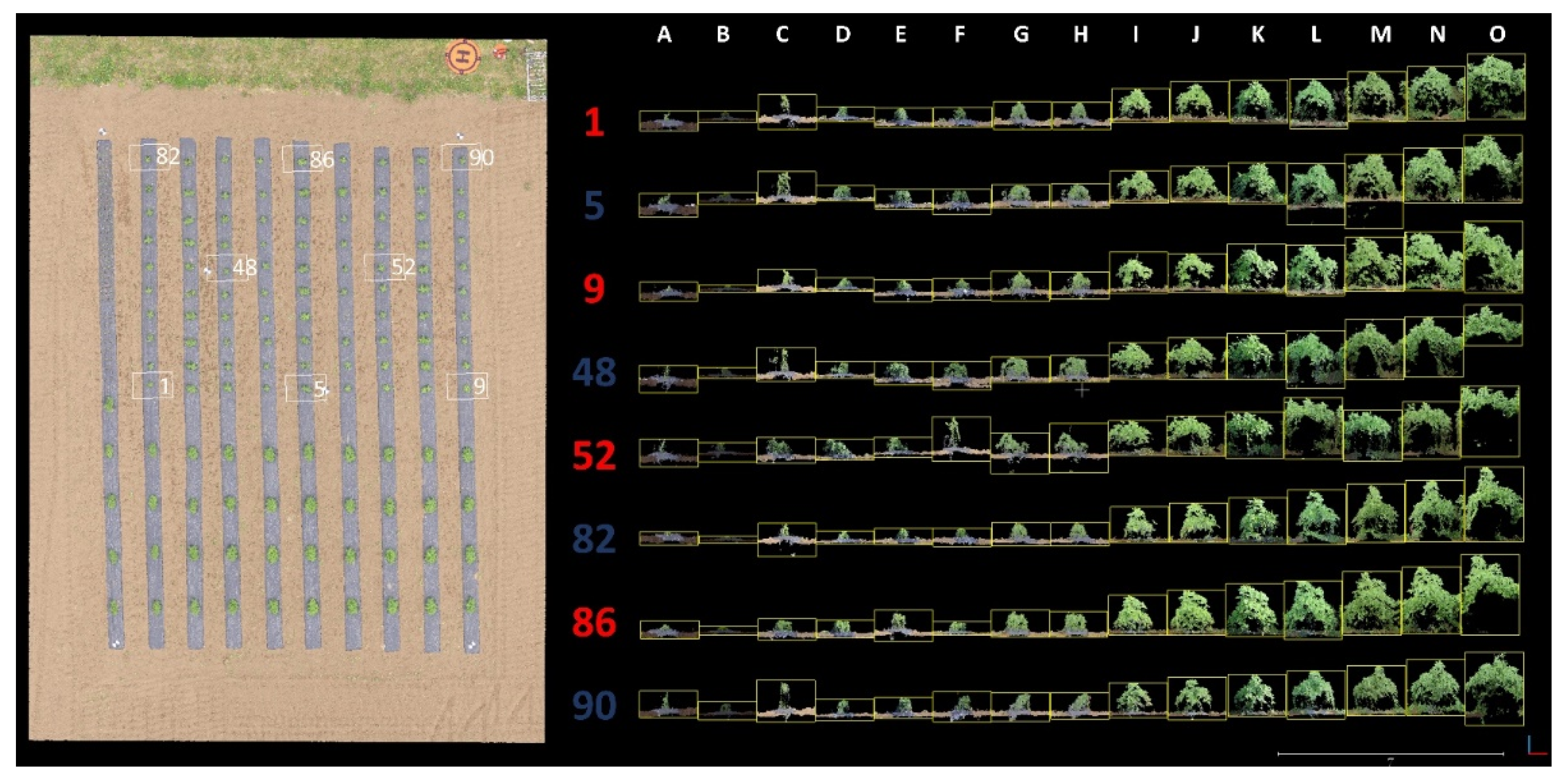
First, the reconstruction quality is fundamental for all follow-up steps. However, the current quality assessment is still operated manually. When it comes to high-throughput phenotyping (HTP) applications in large-scale fields, this tedious manual step remains an ongoing challenge. One possible semi-automated solution is cropping each plot over time and detecting sudden changes [14]. The detected sudden change points may meet bad reconstruction quality (e.g., Column C in Figure A1, Appendix A). This idea relies on a handy tool for batch-cropping time series point cloud data, but no such tool has been developed yet.
Second, agronomists and breeders are often only interested in a specific area in the entire field, called the region of interest (ROI) [13]. ROIs can be individual plots with different treatments or production organs, such as lettuce leaves, broccoli flowers, sorghum, and rice head. It is a standard operation to extract corresponding ROIs from the whole field for better data management. Alternatively, the whole field is split into several small parts, facilitating organ detection and segmentation. Currently, this cropping step is still manually operated by geographic information system (GIS) software [15], for example, ArcGIS (Esri, Redlands, CA, USA) and QGIS (www.qgis.org, accessed on 1 June 2021). When it comes to HTP in the large field, although GIS-programmable APIs and the “drone-dataflow” toolbox [13] in MATLAB (MathWorks Inc., Natick, MA, USA) are available for batch processing, it requires professional programming and GIS operating skills. These tools are still difficult to directly focus on agriculture-related output.
Third, limited by the complex field conditions, the concatenated DOM often has image quality diminution compared to raw images [16]. A technique called reverse calculation, which links the same place from DOM back to relative raw UAV images, has attracted extensive interest [8,16,17,18], as it not only improves the ground cover estimation accuracy [8] but also enables small-organ (e.g., sorghum head) detection tasks from UAV images [17,18]. However, previous studies have applied Pix4D, while Metashape is also used in many plant phenotyping studies [19,20,21,22], but these techniques have not been examined and supported yet. Furthermore, there are no handy tools available for agronomists and breeders without professional programming skills.
The objective of the proposed software package (easy intermediate data processor (EasyIDP), MIT license) is to address previously identified difficulties and decrease the workload in intermediate data processing for agronomists and breeders, including (1) cropping both large PCD and DOM to small parts by given ROIs; (2) reverse-calculating given ROIs on the corresponding place on raw UAV images for both Pix4D and Metashape projects; and (3) testing the accuracy and performance of the developed functions using six different plots with various crops.

2. Materials and Methods

2.1. Study Sites and Image Acquisition

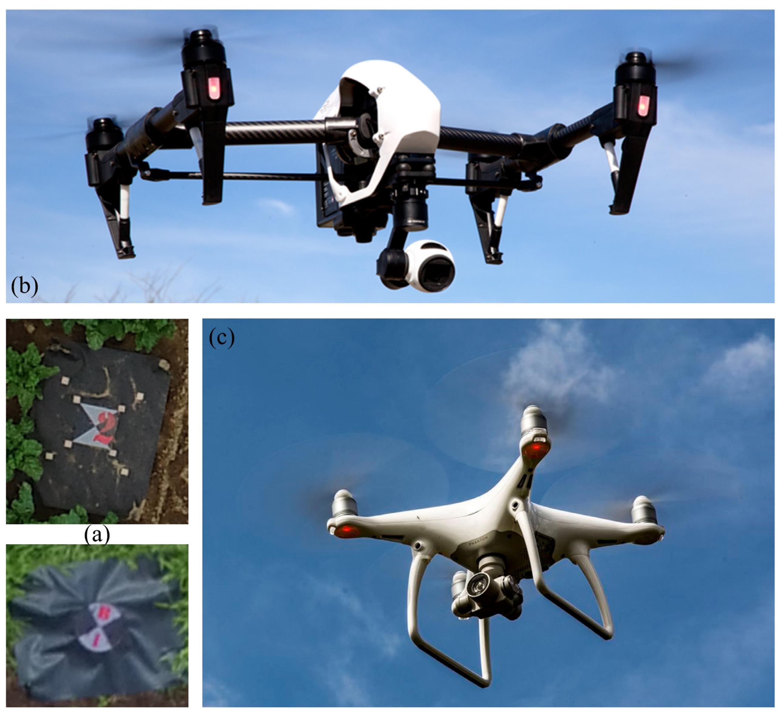
Six field datasets with different characteristics of crops were selected to develop and test the performance of the proposed package (Table 1). For datasets 1–3 and 6, several coded targets were set in the field before sowing crops as GCPs (Figure A2a in Appendix B). For dataset 5, three distinguishable corners of the field were used as GCPs. For dataset 4, no GCP was picked. All the GCPs were measured using Hemisphere RTK differential GNSS devices (Hemisphere GNSS) to obtain the precise geographical position for producing the georeferenced digital orthomosaic (DOM) and DSM in the later SfM-MVS procedure.
DJI Inspire 1 (Figure A2b in Appendix B) with an FC550 onboard camera (SZ DJI Technology Co., Ltd., Shenzhen, China) and DJI Phantom 4 (Figure A2b in Appendix B) with FC6310 and FC6310S onboard cameras (SZ DJI Technology Co., Ltd., Shenzhen, China) were used to acquire images with a flight height of 30/50 m. The flight plan was designed using a double-grid style with LitchAPP software (VC Technology Ltd., London, UK), with >90% overlap of the pictures with the front and sides.

2.2. Three-Dimensional Reconstruction by SfM-MVS

Two commercial software programs, Pix4Dmapper Pro (Pix4D, S.A., Prilly, Switzerland) and Agisoft Metashape Pro (Agisoft LLC, St. Petersburg, Russia), were used to process all six fields. Most of the parameters were used as software defaults. All the GCPs and their geographical positions were detected by built-in software tools. For each GCP, its related position in four UAV raw images was manually picked.
Agricultural fields are often flat and homogenous, and it is hard to provide enough visual information for camera calibration optimization [23], which often causes curved ground. To minimize this effect, for the initial processing procedure in Pix4D, the “calibration method” was set to “alternative” and “camera optimization” was set to “all prior” [23]. For the “align photos” procedure in Metashape, the “reference preselection” was selected and “generic preselection” was deselected, as mentioned in its user manual [24] (p. 30).
Sometimes, the z-axis (height) scale was incorrect. After processing aligned photos, the derived camera height was checked. If the derived height was not close to the actual flight height, the image height was manually modified. In addition, z-axis accuracy was set to 0.05 m to fix the flight height, helping correct the z-axis scaling issue.
The configuration of the computer used in this manuscript is as follows: Intel(R) Core (TM) i9-7980XE CPU @2.60GHz, 64GB RAM, two NVIDIA GeForce GTX 1080Ti GPUs, and Windows 10 Pro, 64-bit operating system.

2.3. ROI Making

The EasyIDP package has no graphical user interface (GUI) for manual ROI marking of all kinds of outputs. Therefore, some external software to mark the ROI on different outputs is required.
Standard GIS software, such as QGIS or ArcGIS, can be used to produce 2D XY polygon shapefiles (*.shp) on the georeferenced GeoTiffs (DOM and DSM; please refer to Guo et al. [25] and https://github.com/oceam/UAVPP/wiki, accessed on 1 June 2021 for guidance on drawing shapes). The missing Z values (height) in the 2D ROI can be extracted from the DSM by EasyIDP. The open source CloudCompare (http://cloudcompare.org, accessed on 1 June 2021) can be used to produce 3D XYZ ROIs by picking several points and exporting them to the .txt file. Please refer to the user manual (https://github.com/HowcanoeWang/EasyIDP/wiki, accessed on 1 June 2021) for detailed tutorials.

2.4. ROI-Cropping Module

The function of this module is cropping ROIs from entire georeferenced GeoTIFF data (DOM and DSM) or point clouds (PCDs). Several external Python packages were used to implement this function, including “tifffile” (https://github.com/cgohlke/tifffile, accessed on 1 June 2021), “pyshp” (https://github.com/GeospatialPython/pyshp, accessed on 1 June 2021), “pyproj” (https://github.com/pyproj4/pyproj, accessed on 1 June 2021), “plyfile” (https://github.com/dranjan/python-plyfile, accessed on 1 June 2021), and “open3d” [26].
For GeoTIFF files, the “tifffile” package was used to read the geo-header data and channel image data. The geo-header data contain the offset, resolution, and geographic projection information. It was used for transforming pixel coordinates into channel images and real-world geographic coordinates. Note that the channel image data were only partially loaded, when necessary, to save the memory usage for large-size GeoTIFFs.
For ROI shapefiles, the “pyshp” package was used to read polygon ROIs from the *.shp files. Ideally, the ROI shapefile was the same geographic projection as the GeoTIFF file. The “pyproj” package was used to deal with inconsistent geographic projections. After properly loading ROIs and GeoTIFFs, the bounding box of ROIs was calculated and transformed to a binary mask to crop the ROIs from the whole field. Finally, the clipped ROIs were saved to the GeoTIFF file for later usage.
The whole GeoTIFF can also be split into regular grids with a given width and height. The cropping module transformed each grid as one ROI and cropped them into small GeoTIFF files without using any GIS software or APIs. This function may benefit data batch preprocessing for deep learning applications, especially on the web server.
For point cloud files, the “open3d” package was used to read their data. The ”plyfile” package was used to fix colors missing for some *.ply files. The point cloud crop function in “open3d” was modified to crop ROIs and saved to a single point cloud file.

2.5. ROI-Reversing Module

The function of this module is projecting ROIs from world coordinates to relative UAV raw images. In this section, the external and internal camera parameters generated from SfM-MVS reconstruction projects were loaded by two internal Python packages, “zipfile” and “xml.” Then, reverse calculation algorithms driven by a pinhole camera model and camera distortion calibration were introduced. Some Python scientific computation packages, such as “numpy” [27], “matplotlib” [28], and “pandas”(https://pandas.pydata.org, accessed on 1 June 2021), were used in this calculation step.

2.5.1. Camera Parameter Loading

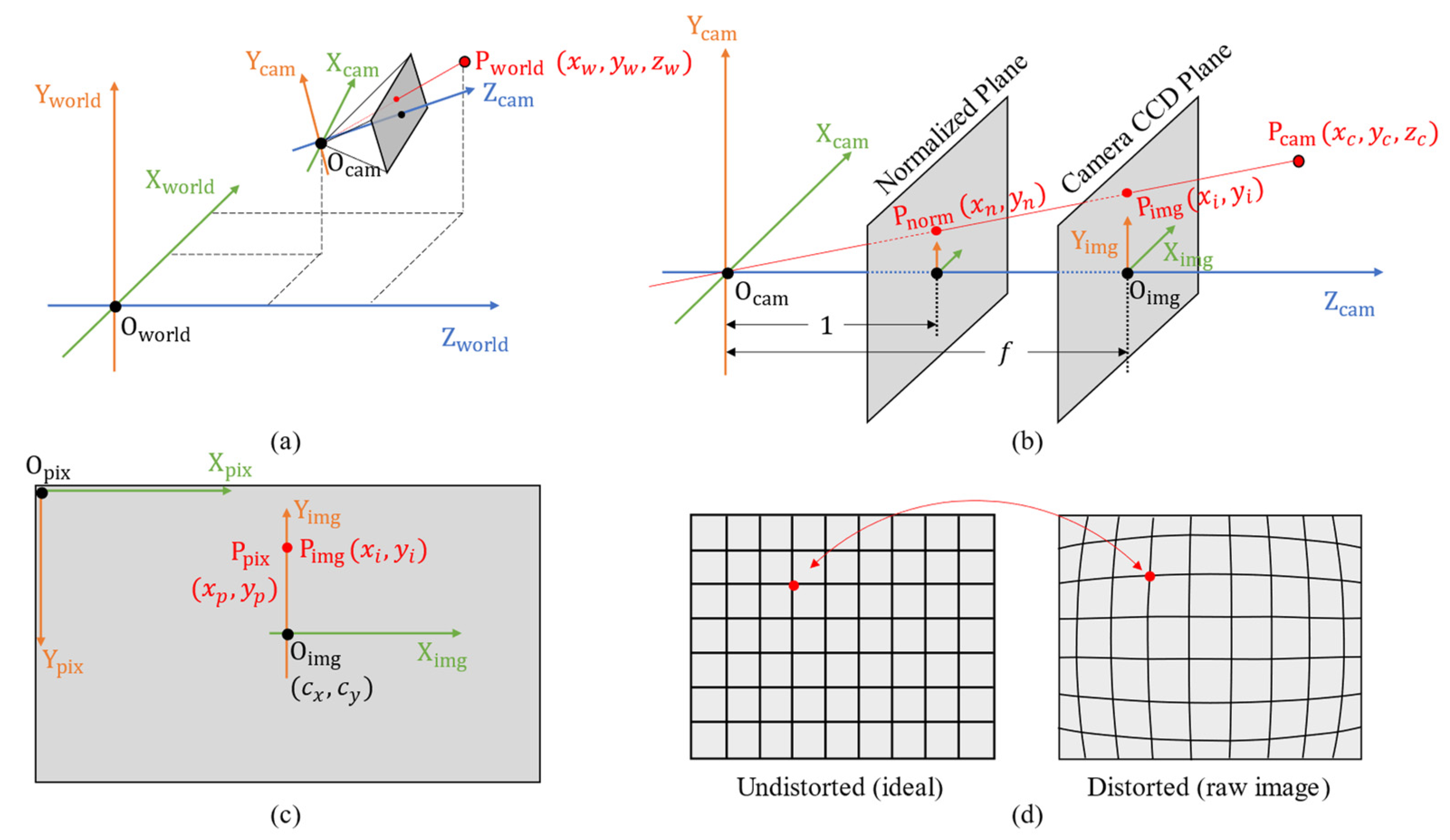
The relationship between field and UAV raw images was built after running SfM-MVS software. It has two main parts, external and internal parameters. The external parameters are different for each raw image, including the camera position (x, y, z) in the real-world coordinate ( O w o r l d , Figure 2a) and the camera rotation (yaw, pitch, roll). The internal parameters describe the characteristics of the sensor and are the same of each raw image, such as focal length, camera charge-coupled device (CCD) size, and lens distortion calibration parameters.
For Metashape projects, all these parameters can be obtained either by calling APIs (professional license required) or by reading zipped .xml files in the project file “project.files/0/chunks.zip/doc.xml.” The EasyIDP package chose the zipped xml way without a professional license. The “zipfile” and “xml” packages were used to unzip and parse these parameters in .xml files.
For Pix4D projects, all these parameters are located in the “pix4d_project/1_initial/params” folder, the “calibrated_internal_camera_parameters.cam,” “calibrated_camera_paramters.txt,” “pmatrix.txt” and “offset.xyz” are loaded as text directly and parsed in the EasyIDP package without any external packages. For more details about these files, please refer to the Pix4D official documentation [29].

2.5.2. Reverse Calculation

The geometry from the real-world coordinate ( O w o r l d ) to image the pixel coordinate ( O p i x ) is shown in Figure 2a–c. There are four coordinate systems. The first is O w o r l d , whose unit is often meter (Figure 2a). The second is the camera coordinate ( O c a m , Figure 2b), which makes the camera position to the origin (0,0,0) of coordinates, and the camera optical axis is used as the z-axis (commonly, the point O i m g is not the center point of plane). The third is the camera CCD coordinate ( O i m g , Figure 2c), whose unit is often millimeter. The last one is the pixel coordinate ( O p i x ), whose origin is the top-left corner in O i m g and the unit is pixel.
Let us assume a point P w o r l d ( x w ,   y w , z w ) in O w o r l d . To transform that point into P c a m ( x c ,   y c ,   z c ) in O c a m (Figure 2a), the 4 × 4 transform matrix T could be derived from the camera position ( t , translational transformation) and camera rotation ( R , rotational transformation):
P c a m = T P w o r l d [ x c y c z c 1 ] = [ R 11 R 12 R 13 t 1 R 21 R 22 R 23 t 2 R 31 R 32 R 33 t 3 0 0 0 1 ] [ x w y w z w 1 ]
where t is the 3 × 1 position matrix and R is the 3 × 3 rotation matrix derived by ( ω , ϕ ,   κ ) from camera rotation parameters (yaw, pitch, roll) [29,30]:
R = R x ( ω ) R y ( ϕ ) R z ( κ ) = [ 1 0 0 0 cos ( ω ) sin ( ω ) 0 sin ( ω ) cos ( ω ) ] [ cos ( ϕ ) 0 sin ( ϕ ) 0 1 0 sin ( ϕ ) 0 cos ( ϕ ) ] [ cos ( κ ) sin ( κ ) 0 sin ( κ ) cos ( κ ) 0 0 0 1 ] = [ cos κ cos ϕ sin κ cos ϕ sin ϕ cos κ sin ω sin ϕ + sin κ cos ω cos κ cos ω sin κ sin ω sin ϕ sin ω cos ϕ sin κ sin ω cos κ cos ω sin ϕ sin κ cos ω sin ϕ + cos κ sin ω cos ω cos ϕ ]
The distance from the normalized plane to the origin O c a m is 1 mm, while the distance from the camera CCD plane to the origin O c a m is focal length f (Figure 2b) in millimeters. The transformation from P c a m ( x c ,   y c , z c ) to normalized plane P n o r m ( x n , y n ) and camera CCD plane P i m g ( x i ,   y i ) can be derived by triangle similarity:
[ x i y i ] = f [ x n y n ] = f [ x c z c y c z c ] = f z c [ x c y c z c ]
To transform P i m g ( x i , y i ) in millimeters to the image pixel coordinate position P p i x ( x p , y p ) in pixels (Figure 2c), the following set of equations should be applied:
[ x p y p ] = [ α x i + c x β y i + c y ] = [ f α x n + c x f β y n + c y ] [ x p y p 1 ] = [ f α 0 c x 0 f β c y 0 0 1 ] [ x n y n 1 ] = K [ x n y n 1 ]
where α and β are the pixel resolution whose unit is pixel/mm and often are the same in pinhole camera models. f α and f β is the focal length in pixels. Notably, Pix4D ( c x ,   c y ) can be obtained directly, while for Metashape [24] (p. 176), ( c x ,   c y ) in the .xml file is not what is defined here; it is the offset to the image center, which actually equals ( 0.5 w + c x ,   0.5 h + c y ) , where w and h are the pixel width and height, respectively.
To sum up Equations (1) to (4), transform P w ( x w ,   y w ,   z w ) directly to P p i x ( x p , y p ) , which can be derived by:
[ x p y p 1 ] = 1 z c [ f α 0 c x 0 f β c y 0 0 1 ] [ x c y c z c ] = 1 z c K [ x c y c z c ] = 1 z c K   T [ x w y w z w 1 ] = P m a t [ x w y w z w 1 ]
where the 3 × 4 matrix P m a t is often called the projection matrix, which can directly transform points in 3D world coordinates to 2D pixel coordinates.

2.5.3. Camera Distortion Calibration

The Equation (5) transformation is idealized, and the distortion caused by the camera lens is neglected (Figure 2d). Several camera calibration parameters are used to correct this distortion, including three or four radial distortion coefficients ( K i in MetaShape and R i in Pix4D) and two tangential distortion coefficients ( P i in MetaShape and T i in Pix4D). Metashape sometimes provides affinity ( B 1 ) and non-orthogonality ( B 2 ) coefficients in pixels. The correction equations for the distorted pixel position ( x p ,   y p ) are as follows:
r = x n 2 + y n 2 x = x n ( 1 + K 1 r 2 + K 2 r 4 + K 3 r 6 + K 4 r 8 ) + P 1 ( r 2 + 2 x n 2 ) + 2 P 2 x n y n y = y n ( 1 + K 1 r 2 + K 2 r 4 + K 3 r 6 + K 4 r 8 ) + P 2 ( r 2 + 2 y n 2 ) + 2 P 1 x n y n x p = c x + x f + x B 1 + y B 2 y p = c y + y f

2.5.4. Performance Evaluation

To evaluate the performance of reverse calculation and identify the factors contributing to the deviation, the lotus field (dataset 5) with a clear plot boundary (pond edges) was used for evaluation. The expected reference results were made manually by LabelMe annotation software (https://github.com/wkentaro/labelme, accessed on 1 June 2021) and were used to compare with those calculated by the EasyIDP reversing module. Three indicators, namely the intersection of union (IoU) performance criterion [31], precision, and recall, were used to evaluate the similarities between the package output (program area) and manual marking (manual area) and could be calculated by (refer to Figure 3 in Tresch et al. [16] for the IoU diagram of each area)
I o U = i n t e r s e c t i o n   a r e a u n i o n   a r e a p r e c i s i o n = i n t e r s e c t i o n   a r e a p r o g r a m   a r e a r e c a l l = i n t e r s e c t i o n   a e r a m a n u a l   a r e a
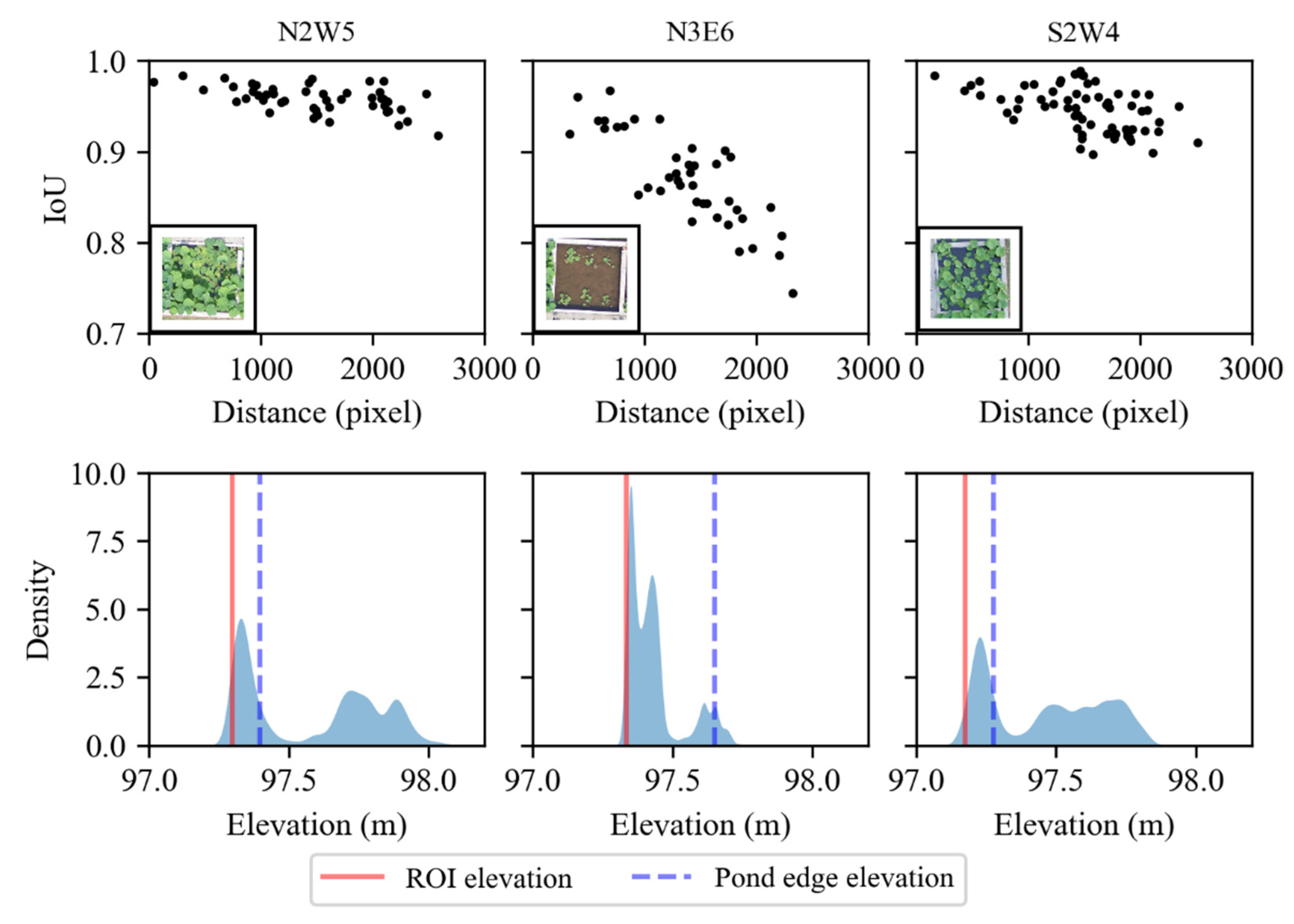
Two kinds of comparisons were involved. For the first one, three plots with different lotus densities (N3E6: sparsest; S2W4: medium sparse; N2W5: densest) were selected, and all related raw images were marked manually. The pixel Euclidean distance from the IoU center to the image center was also calculated, and the relationship between the indicator values and Euclidean distance was simply discussed. Second, for each plot, the smallest IoU Euclidean distance raw image was selected to mark the manual reference, and the overall trend of the indicators was simply analyzed.

2.6. Implementation

The cropping and reversing modules mentioned above were implemented into a Python package called EasyIDP using the MIT license. The source code can be downloaded from https://github.com/HowcanoeWang/EasyIDP, accessed on 1 June 2021. For specific package documentation, please refer to https://github.com/HowcanoeWang/EasyIDP/wiki, accessed on 1 June 2021. Although the source codes were cross-platform owing to the characteristics of the Python language, they were programmed and tested on a Windows 10 64-bit platform and an Intel CPU with a math kernel library (MKL). More than 8 GB RAM and 3.0 GHz CPU are recommended for better performance.

3. Results

As mentioned in the introduction, intermediate data processing has three points that need to be solved: (1) cropping the point cloud to small sectors of a given ROI; (2) cropping the given ROI from GeoTiffs; and (3) reverse-calculating the ROI to the corresponding position on raw UAV images. PCD and GeoTiff cropping was integrated into the cropping module, while reverse-calculating was implemented by the reversing module. The accuracy evaluation by manually marked references was also included.

3.1. ROI Cropping

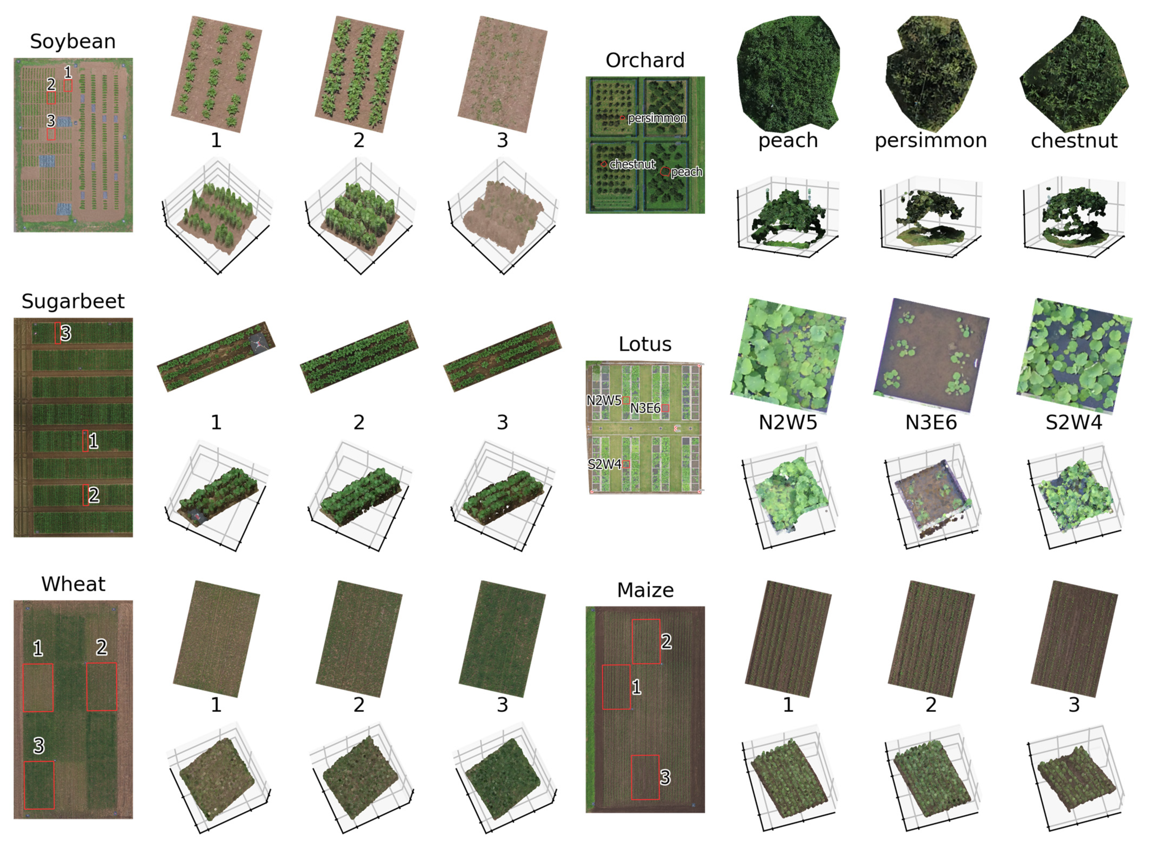
Some examples of the cropping function are shown in Figure 3. Three ROIs were randomly chosen for each dataset with different cultivars or treatments. For each image group (dataset), the left side with the plot name was the DOM generated by MetaShape. The positions of randomly selected ROIs in the field are displayed on it. The first row of each group is the cropped sector of the DOM, while the second row is the cropped point cloud. According to this figure, similar patterns between PCD and DOM sectors were observed, and the cropping module worked, as expected.

3.2. ROI Reversing

3.2.1. Reversing Results for Pix4D and Metashape

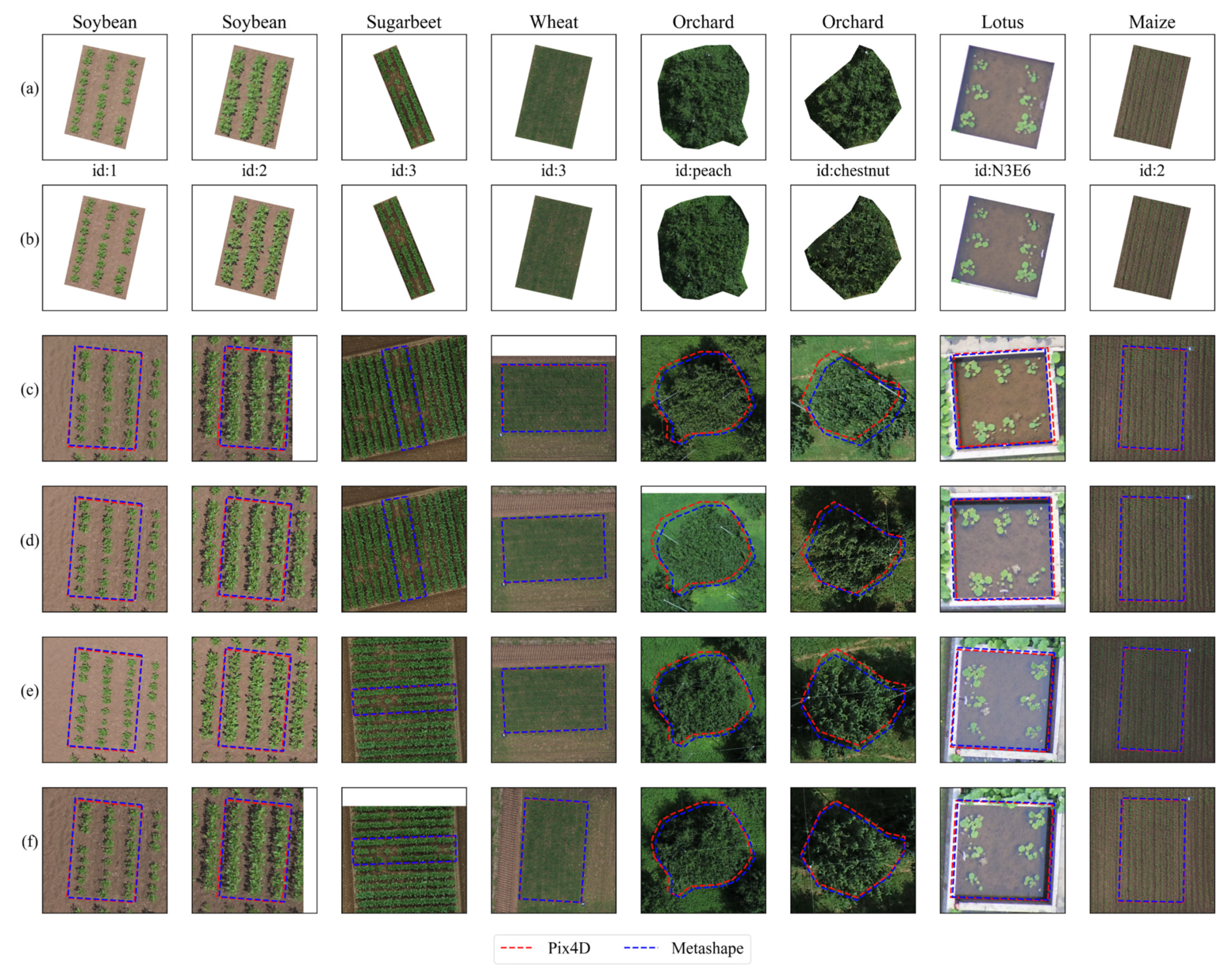
Some parts of the reverse calculation are shown in Figure 4. The first and second rows are the ROIs clipped from the DOM generated by Pix4D and Metashape, respectively. Some slight differences between the Pix4D- and Metashape-produced DOM were observed for the Orchard field (Figure 4, columns 5 and 6). Pix4D was clearer for canopy details. The other rows are relative positions on raw UAV images; broken red lines represent Pix4D results, and blue ones represent MetaShape results. A slight deviation was observed on those fields with GCPs (<5 pixels). The Orchard field without GCPs had bigger deviations, but the target crown was still covered by reversed results correctly. In addition, the deviations were variant to different view angles (raw image positions, different rows in Figure 4c–f). Nevertheless, compared with the ROI size, these deviations should have no significant impact on the obtained results.

3.2.2. Reverse Accuracy Evaluation

To quantitatively evaluate the performance of reverse calculation, the dataset 5 Lotus field with a clear plot boundary was used to examine the accuracy by manually drawn references. There were two different comparisons involved. The first one was single plot reversing on all raw images, while the second one was all plots reversing on only single centered images.
The results of the performance evaluation for the first kind of comparison are shown in Figure 5. For plots N2W5 and S2W4 with a complex canopy, most of the IoU values were over 90%, and surprisingly, for the simplest and sparse-canopy plot N3E6, although the IoU values were still greater than 75%, the performance was moderate. The reason may be the automatic z value (height) calculation of ROIs. The z values used for ROIs were the mean height of the ROI (ROI elevation, solid red lines), while for manually marked references, it was the height of the plot edge. By manually picking some points of the edge in QGIS, the height of the pond edge was represented in broken blue lines. The plot N3E6 had almost 25 cm differences between the auto mean ROI elevation and the referenced pond elevation, mainly caused by the transparent water. The 3D reconstruction built the bed mud rather than the water surface for this plot, showing that the ROI height selection is of great importance for the reverse calculation accuracy. Another trend in this figure is that the IoU decreased with the distance increasing from the ROI center to the photo center. This result means that the ROI position on raw UAV images (the view angle of raw UAV images) also affects the reverse calculation accuracy.
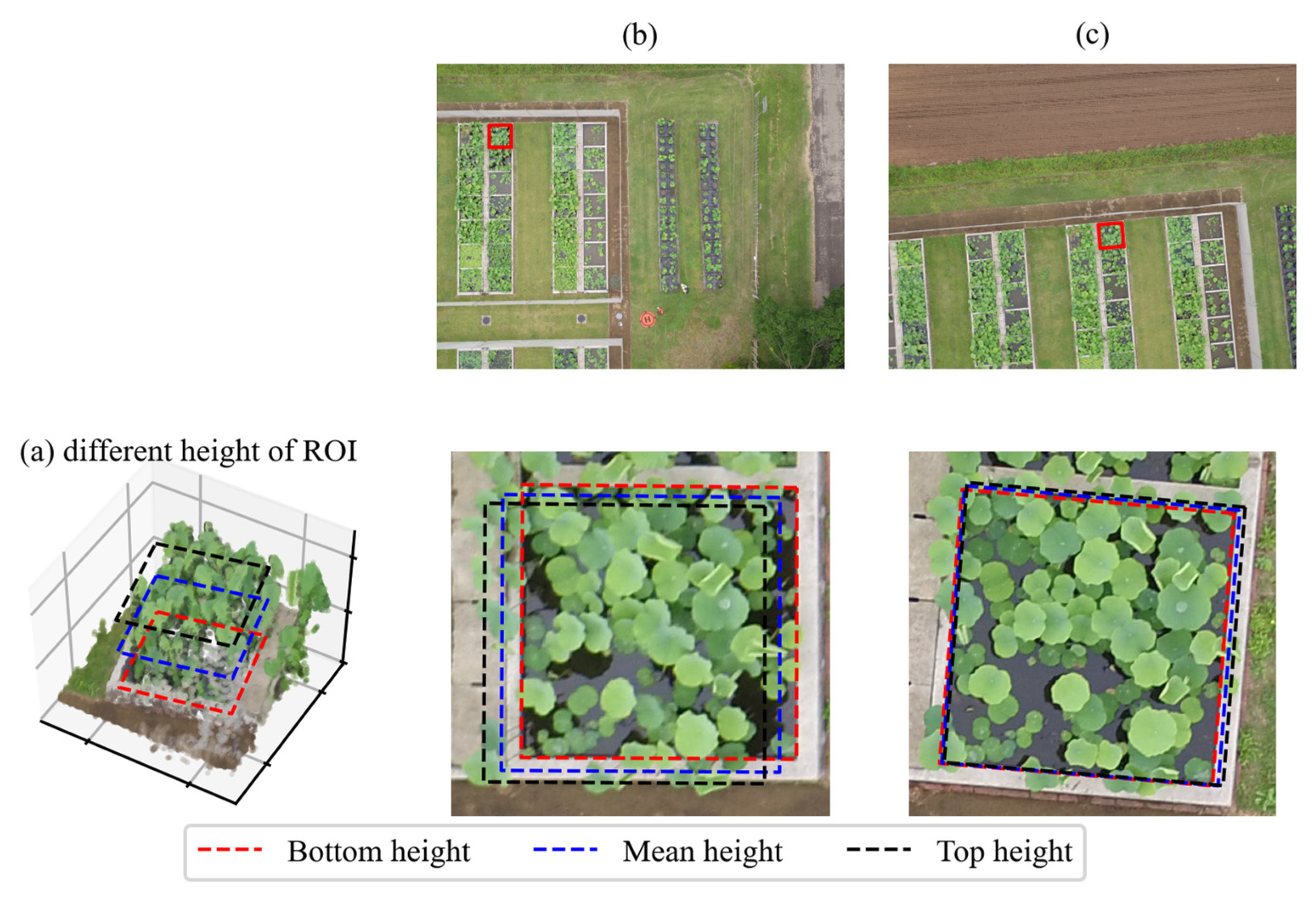
The effects of ROI height selection and its position are shown in Figure 6. Three different heights were used. The broken red lines “bottom height,” m e a n ( Z p 5 ) , were the mean of all points <5th percentile within the ROI. The blue broken lines “mean height,” m e a n ( Z ) , were the mean of all points in the ROI. The black broken lines “top height,” m e a n ( Z p 95 ) , were the mean of points >95th percentile within the ROI (Figure 6a). The closer the reversed ROI to the raw image center, the fewer the deviations caused by different ROI heights (Figure 6b,c). Figure 5 shows that once the pixel distance to the image center was smaller than 800 (the size of the image was 4608 × 3456 pixels), even the moderate-performance plot N3E6 could achieve an IoU greater than 90%. Hence, to minimize the unsuitable ROI elevation selection effects, ROI-centered raw images (like Figure 6c) are recommended. This idea of choosing a centered raw image has also been applied by some studies that used reverse calculation [16,17].
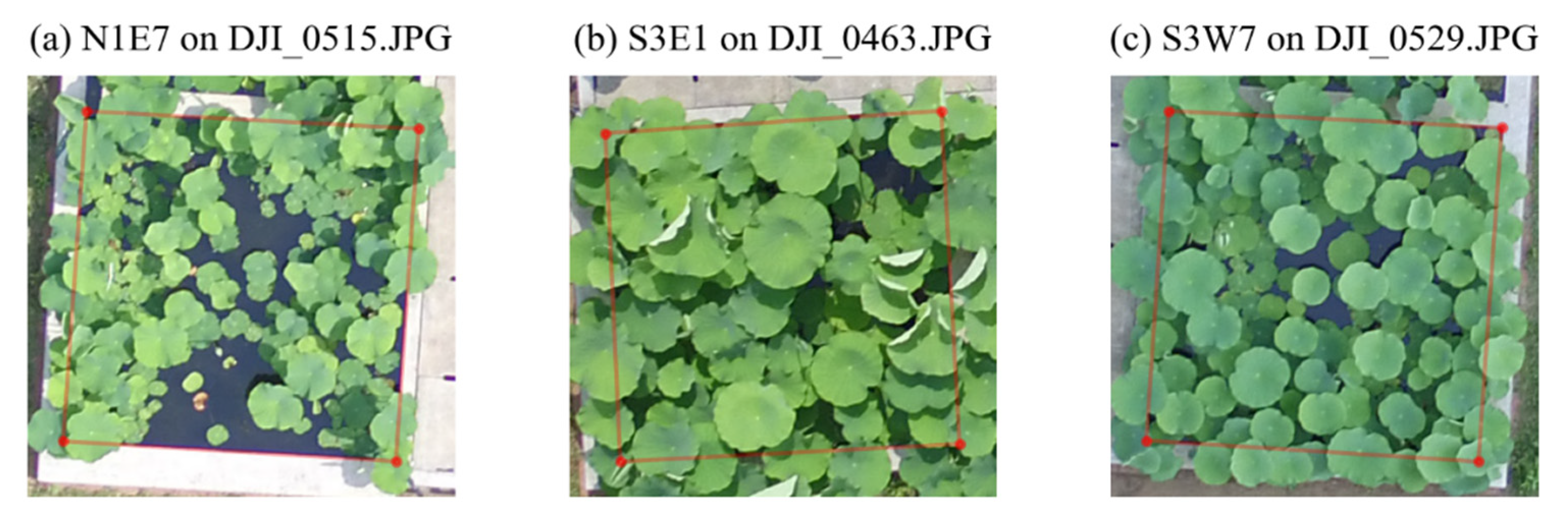
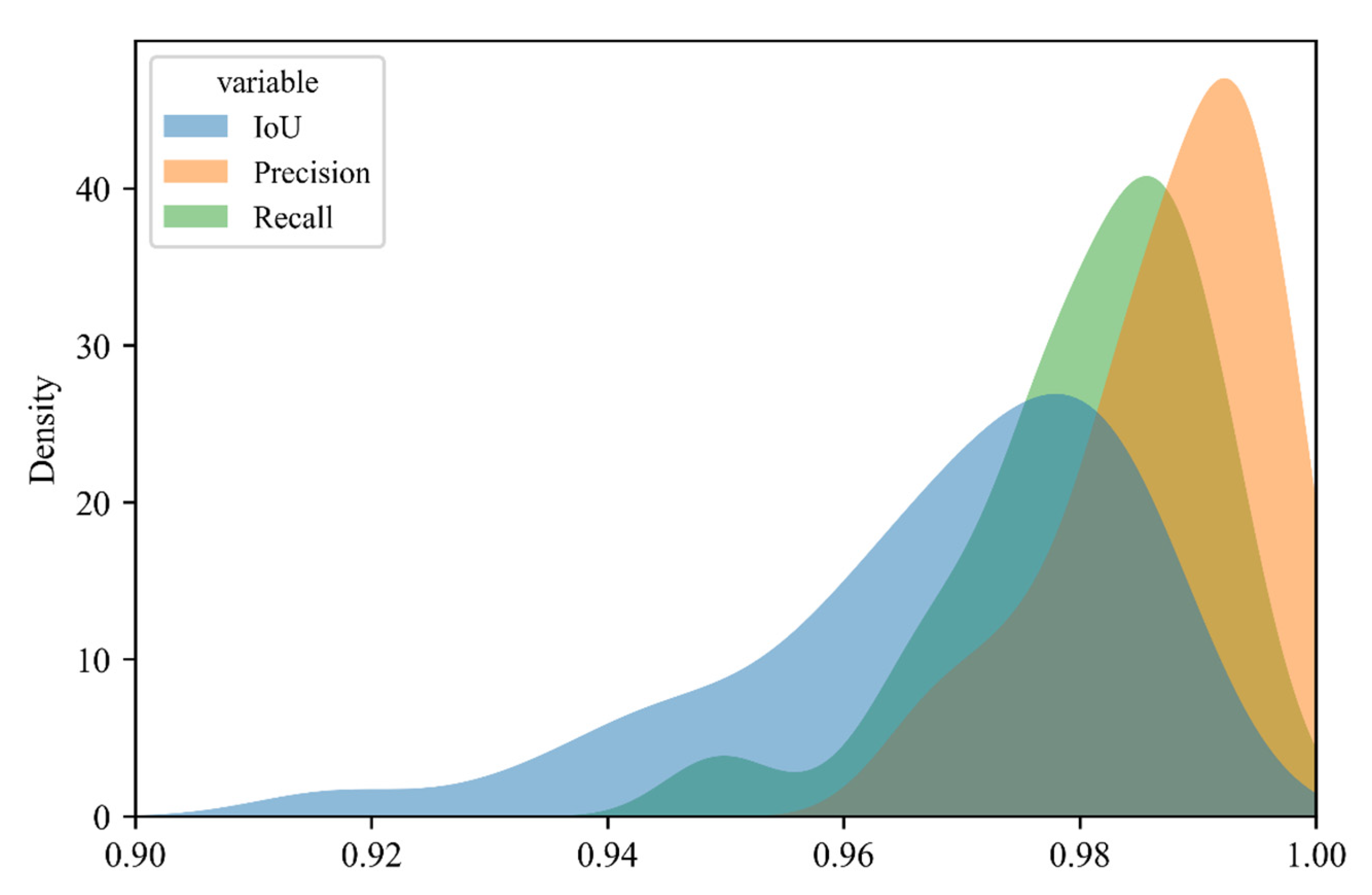
For the second kind of comparison of all 112 plots, only ROI-centered raw images were selected, and the referenced results were marked manually. The distributions of the accuracy assessment indicators are shown in Figure 7. The peaks were around 98%, while the minimum value was still greater than 90%. Considering the difficulties in manual marking in some plots where all corners were covered in leaves and were non-identical (Figure A3 in Appendix C), the reverse transformation accuracy was determined to be acceptable.

4. Discussion

4.1. Reconstruction Quality Control and Assessment in Agriculture

Good reconstruction quality by photogrammetry is fundamental for plant phenotyping accuracy. Furthermore, it is challenging to ensure the quality of open-field agriculture. The core algorithm SfM assumes the object is a rigid body with enough distinguishable feature points. However, in open-field agriculture, complicated plant structures can be deformed easily by wind, and continuous crop canopies with homogeneous surfaces make processing difficult. For horizontal (xy plane) adjustment, one common solution is properly setting GCPs in the field. The spatial distribution should be paid more attention to than the number [10]. In most practices, four corners and one or two in the center could be the most cost-effective way. For vertical (elevation or z-axis) adjustment, it is recommended to check the estimated flight height in software. When a significant deviation to the actual flight height is observed, manually specifying the flight height in software is a possible solution. Some other methods, such as oblique photographs [32] and vertical scalebar setting, such as GCP cube, e.g., magic cube [33], are also applicable.
It is still unavoidable to assess the reconstruction quality manually, even though the above operations have been performed. Generally, the layering problem caused by mismatching in the point cloud should be checked. Partially, the quality of each plant in point clouds and the DOM should also be examined one by one. Hence, for HTP in a large-scale open field, previous time-consuming manual assessment is now becoming a bottleneck for practical applications. One possible semi-automated solution is that cropped ROIs follow the time. Here, the data published in [14] were used as an example to demonstrate this concept. In Figure A1 of Appendix A, a sudden global change in column C (date) is observed as a system error. Moreover, for 52F, 52L, and 86E, sudden individual changes are observed as random errors. These error points indicate the potential imperfect reconstruction quality and need manual assessment, and other cases can be omitted. The results in Figure 3 show that the developed EasyIDP has the ability to crop ROIs correctly. In addition, it opens the door to decrease the workload in quality assessment. Nevertheless, at the current stage, these sudden change detections have not been implemented. An automatic sudden-change-detection pipeline based on the EasyIDP cropping module should be developed in the future.

4.2. Whole DOM Cropping to Small Parts

Object detection and segmentation at different levels are also basic operations in plant phenotyping. At the plot level, agricultural experiments often set different treatments by plot. Hence, cropping the entire field by the plot range decreases the workload in both phenotypic calculation and data management. In addition, at the individual or organ level, this touches the key point in precision agriculture and makes monitoring and predicting crop status and yield more accurate, for example, using computer vision or machine learning algorithms to estimate the size of whole lettuce [34], broccoli flowers [35,36], sorghum, and rice head [17,18,37]. Operating these algorithms directly on the whole-field DOM is often impossible because the memory requirement for some algorithms increases exponentially with the image size.
In both cases, splitting the whole DOM into small sectors, either by ROIs of the plot boundary or by regular generated grids, is necessary for the data preprocessing step. Currently, this step is manually operated by standard GIS software, such as ArcGIS or QGIS. For HTP, the batch operation demand can also be satisfied by the GIS API or the “drone-dataflow” toolbox of MATLAB [13]. However, using these tools requires professional GIS or programming skills. Moreover, in our pre-experiment, their memory cost for a large DOM is still numerous. It is still difficult for users to focus on agriculture-related outputs.
The developed EasyIDP tool showed acceptable cropping results (Figure 3). Using a partial load technique supported by the “tifffile” package, the memory cost is acceptable for large-field DOM data. For example, cropping a 10 GB DOM file to small grids only costs a few lines of code, 0.5 GB memory, and 10 min.

4.3. Reverse Calculation

Using previous quality control operations mentioned in Section 4.1, even though the whole field looks good in general, the connection boundary between two raw images projected on the DOM often has problems, which is caused by complex sunlight and wind conditions. One idea is optimizing the DOM concatenation method, changing those connection boundaries outside plots or ROIs [38]. An alternative idea is giving up optimizing the DOM and finding the relative position on the raw image directly, named reverse calculation [8,16,17]. Though these studies have shown its potential, the detailed calculation algorithm and its accuracy have never been mentioned.
In our results, Figure 4 shows that reverse calculation works on both Pix4D and MetaShape outputs. Only slight deviations are observed between the two software programs. The deviations become larger for the Orchard field without a GCP. Moreover, these differences are acceptable compared to the size of the ROI. The accuracy of reverse calculation on all available raw images was analyzed, and the results are shown in Figure 5. Though generally, an acceptable result is observed on most raw images, the height of the ROI and its positions on raw images significantly affect the accuracy. Their impacts are visualized in Figure 6; the closer the reversed ROI to the raw image center, the smaller the deviation caused by different heights. Once only those closest raw images are chosen, as many studies have done [8,16,17], the accuracy indicators can reach 0.95 or more.
Reverse calculation can also be used to decrease the workload in training data annotation, especially for current popular deep learning applications in agricultural research [36,37,39]. A massive amount of annotations on training images is required to avoid overfitting and ensure the robustness of the deep learning model [18]. Unfortunately, it is hard to use available computer vision annotation databases (e.g., ImageNet [40] and COCO [41]) directly for specialized agricultural tasks. Data annotation is still unavoidable for most plant phenotyping applications [42,43]. One solution is data augmentation. The annotated data are applied by rotation, zooming, flipping, contrast-modifying, and other computer vision algorithms as new annotation data [44], applied in some agricultural deep learning studies [36,45]. However, this image-processing-based data augmentation has failed in many cases and needs smart choices [46]. Another solution is collecting images from the real world from different view angles. Hence, Beck et al. [47] proposed an automatic indoor robotic annotation system to collect natural augmented crop training data in agriculture systems. However, such a device is hard to apply under open-field conditions.
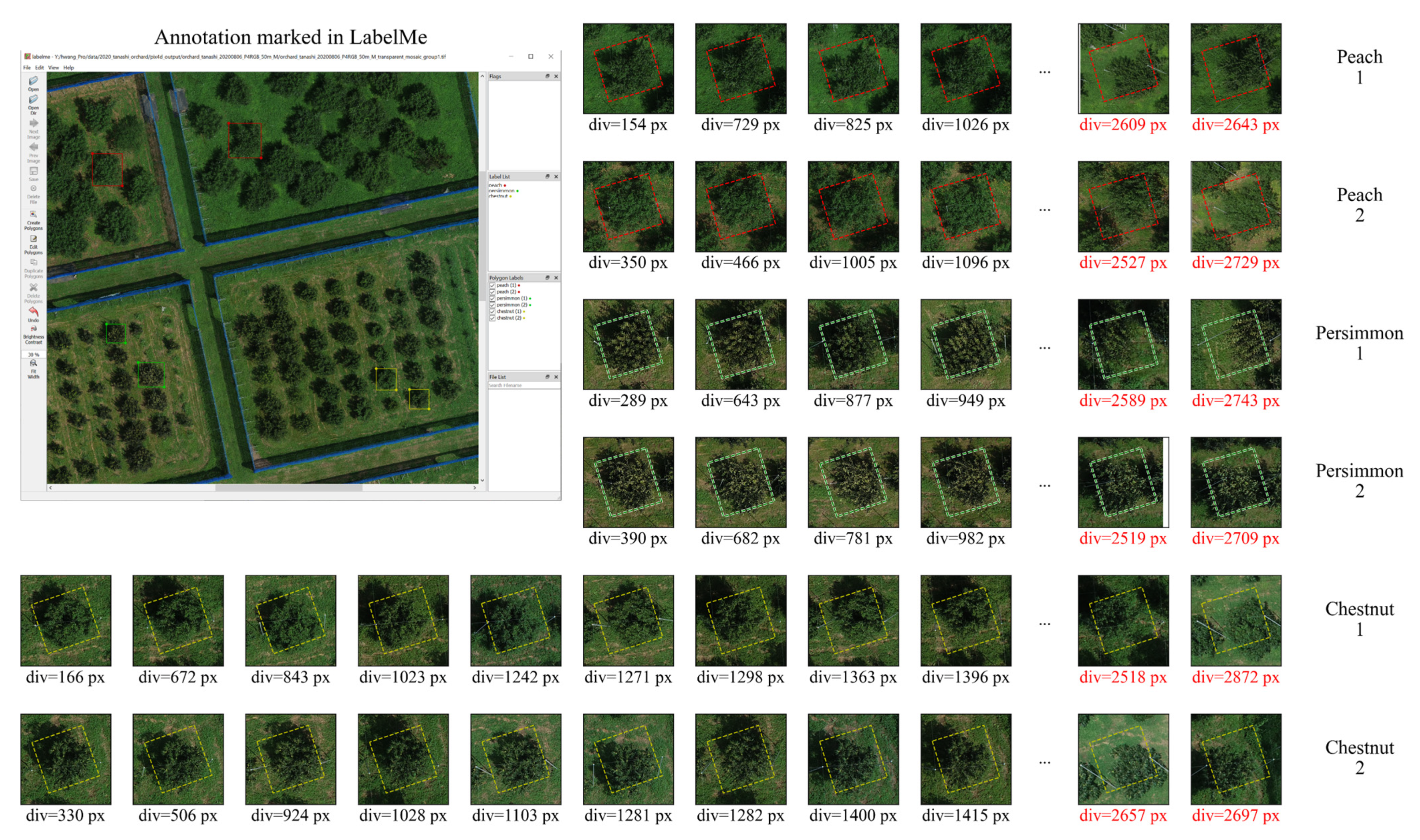
Reverse calculation builds a bridge between real-world and all raw UAV images, which naturally contain abundant view angles (rotation in 3D) and environmental conditions (sunlight, cloud shadow, soil color of different wetness). Figure 8 and Figure 9 exemplify how the idea works for decreasing the workload of data augmentation by reverse calculation at the individual and the organ level, respectively. In both cases, only six rectangle annotations (12 clicks) are labeled by LabelMe on the DOM directly. Then, these annotated rectangles are reversed to all available raw images. Moreover, they are sorted by the distance to the image center. When the object is big enough (Figure 8), such as fruit trees, the farthest is still acceptable for most cases, while it is another story at the organ level for lotus flowers (Figure 9). In both cases, for each annotation on the DOM, at least 10 usable annotations on raw images can be found with various view angles and light conditions.
This data annotation by reverse calculation is not the across-the-board panacea and has some potential limitations. The high quality of 3D reconstruction by SfM is fundamental. Based on that, an object that has a large area (plot level), has a flat terrain or surface (fixed object top height), and is solid (hard to shake by wind) should achieve acceptable results. For example, as our pre-experiment showed, for the sorghum head, which is small and easily affected by wind, the result is far beyond acceptable to use.
All the previously mentioned data augmentation methods share the same idea of automatically enlarging labeled annotation data. Another concept to decrease the labeling workload is to increase the quality and representativeness of each labeled data item, for example, by weakly supervised learning [48], active learning [18,49], generative adversarial networks (GANs) generate synthetic data [50].

4.4. Future Works

The EasyIDP package is currently still a pre-release and under construction for more features. Many aspects could be further modified and developed. Currently, only two commercial software programs, Pix4D and MetaShape, are supported. There are still some other open source programs not supported yet; for instance, OpenDroneMap (www.opendronemap.org, accessed on 1 June 2021) and VisualSfM (http://ccwu.me/vsfm, accessed on 1 June 2021) have also been used in some agricultural phenotyping studies [5,51,52]. In addition, the EasyIDP package is Python script based, which requires users to have some fundamental knowledge about Python programming. The GUI could be developed for easier use. Further, as a tool only for intermediate data preprocessing, this tool can be applied for more advanced open-field agriculture phenotyping, such as decreasing the workload for deep learning training data annotation, predicting the best harvest time, or assisting the cultivar selection for breeders.

5. Conclusions

EasyIDP, a Python package, was proposed to decrease the workload in several manual operation tasks for HTP in large open fields, especially for assessing reconstruction quality and cropping ROIs from the whole field by GIS software. Meanwhile, the reverse calculation used in many studies for both Pix4D and Metashape was also included. The results showed that this tool works, as expected, on both cropping tasks and reversing tasks on both software programs for a variety of crops. Manually marked references validated the reverse calculation accuracy. The effects of ROI height selection and reversed ROI position were discussed. This tool also shows great potential for decreasing the data annotation workload in machine learning applications.

Author Contributions

H.W. and W.G. conceived the ideas and designed the methodology; W.G. collected UAV images; H.W. obtained the outputs of SfM-MVS, programmed the package, and analyzed the data; Y.D. and Y.S. contributed to the part of DOM cropping and annotation transformation; and Y.K. and S.N. supervised this study. All authors discussed, wrote the manuscript, and gave final approval for publication. All authors have read and agreed to the published version of the manuscript.

Funding

This study was partially funded by the JST AIP Acceleration Research “Studies of CPS platform to raise big-data-driven AI agriculture”; the SICORP Program JPMJSC16H2; CREST Programs JPMJCR16O2 and JPMJCR16O1; the International Science & Technology Innovation Program of Chinese Academy of Agricultural Sciences (CAASTIP); and the National Natural Science Foundation of China U19A2061.

Institutional Review Board Statement

Not applicable.

Informed Consent Statement

Not applicable.

Data Availability Statement

Not applicable.

Acknowledgments

We thank the technical staff of the Institute for Sustainable Agro-ecosystem Services (ISAS) for orchard and lotus field management and Kunihiro Kodama from the Laboratory of Plant DNA Analysis, Kazusa DNA Research Institution, Chiba, Japan for meaningful discussions about MetaShape API usage.

Conflicts of Interest

The authors declare that they have no competing interests.

Abbreviations

DOMDigital orthomosaic
DSMDigital surface model
GANGenerative adversarial network
GCPGround control point
GISGeographic information system
GUIGraphical user interface
HTPHigh-throughput phenotyping
LiDARLight detection and ranging
MKL(Intel) Math kernel library
MVSMulti-view stereo
PCDPoint cloud
RGBRed, green, and blue
ROIRegion of interest
RTKReal-time kinematic
SfMStructure from motion
UAVUnmanned aerial vehicle

Appendix A

Examples of reconstruction quality assessment by point cloud cropping; the data are published in [14].
Figure A1. Examples of time series point cloud cropping. Each column is a flight during the growing season.
Remotesensing 13 02622 g0a1

Appendix B

Figure A2. Ground control point (GCP) and unmanned aerial vehicle (UAV) systems used in the field. (a) Square and circle GCPs, (b) DJI Inspire 1, and (c) DJI Phantom 4 (V1 and V2 share a similar appearance).
Remotesensing 13 02622 g0a2

Appendix C

Figure A3. Complex examples for manually marking the expected (reference) transformation results. The plot corner or edge is partly or mostly covered by lotus leaves and cannot be identified.
Remotesensing 13 02622 g0a3

References

  1. Wu, S.; Wen, W.; Xiao, B.; Guo, X.; Du, J.; Wang, C.; Wang, Y. An Accurate Skeleton Extraction Approach From 3D Point Clouds of Maize Plants. Front. Plant Sci. 2019, 10, 248. [Google Scholar] [CrossRef] [PubMed] [Green Version]
  2. Ten Harkel, J.; Bartholomeus, H.; Kooistra, L. Biomass and Crop Height Estimation of Different Crops Using UAV-Based Lidar. Remote Sens. 2019, 12, 17. [Google Scholar] [CrossRef] [Green Version]
  3. Jin, S.; Su, Y.; Song, S.; Xu, K.; Hu, T.; Yang, Q.; Wu, F.; Xu, G.; Ma, Q.; Guan, H.; et al. Non-Destructive Estimation of Field Maize Biomass Using Terrestrial Lidar: An Evaluation from Plot Level to Individual Leaf Level. Plant Methods 2020, 16, 69. [Google Scholar] [CrossRef]
  4. Sun, S.; Li, C.; Chee, P.W.; Paterson, A.H.; Jiang, Y.; Xu, R.; Robertson, J.S.; Adhikari, J.; Shehzad, T. Three-Dimensional Photogrammetric Mapping of Cotton Bolls in Situ Based on Point Cloud Segmentation and Clustering. ISPRS J. Photogramm. Remote Sens. 2020, 160, 195–207. [Google Scholar] [CrossRef]
  5. Zhu, B.; Liu, F.; Xie, Z.; Guo, Y.; Li, B.; Ma, Y. Quantification of Light Interception within Image-Based 3D Reconstruction of Sole and Intercropped Canopies over the Entire Growth Season. Ann. Bot. 2020, 126, mcaa046. [Google Scholar] [CrossRef] [PubMed] [Green Version]
  6. Jay, S.; Rabatel, G.; Hadoux, X.; Moura, D.; Gorretta, N. In-Field Crop Row Phenotyping from 3D Modeling Performed Using Structure from Motion. Comput. Electron. Agric. 2015, 110, 70–77. [Google Scholar] [CrossRef] [Green Version]
  7. Zermas, D.; Morellas, V.; Mulla, D.; Papanikolopoulos, N. 3D Model Processing for High Throughput Phenotype Extraction—The Case of Corn. Comput. Electron. Agric. 2020, 172, 105047. [Google Scholar] [CrossRef]
  8. Duan, T.; Zheng, B.; Guo, W.; Ninomiya, S.; Guo, Y.; Chapman, S.C. Comparison of Ground Cover Estimates from Experiment Plots in Cotton, Sorghum and Sugarcane Based on Images and Ortho-Mosaics Captured by UAV. Funct. Plant Biol. 2017, 44, 169. [Google Scholar] [CrossRef]
  9. Hu, P.; Chapman, S.C.; Zheng, B. Coupling of Machine Learning Methods to Improve Estimation of Ground Coverage from Unmanned Aerial Vehicle (UAV) Imagery for High-Throughput Phenotyping of Crops. Funct. Plant Biol. 2021, 48, 766–779. [Google Scholar] [CrossRef]
  10. Oats, R.; Escobar-Wolf, R.; Oommen, T. Evaluation of Photogrammetry and Inclusion of Control Points: Significance for Infrastructure Monitoring. Data 2019, 4, 42. [Google Scholar] [CrossRef] [Green Version]
  11. Feldman, A.; Wang, H.; Fukano, Y.; Kato, Y.; Ninomiya, S.; Guo, W. EasyDCP: An Affordable, High-throughput Tool to Measure Plant Phenotypic Traits in 3D. Methods Ecol. Evol. 2021. [Google Scholar] [CrossRef]
  12. Young, D. Ucdavis/Metashape: Easy, Reproducible Metashape Workflows. Available online: https://github.com/ucdavis/metashape (accessed on 2 June 2021).
  13. Mortensen, A.K.; Laursen, M.S.; Jørgensen, R.N.; Gislum, R. Drone dataflow—A MATLAB toolbox for extracting plots from images captured by a UAV. In Precision Agriculture ’19; Wageningen Academic Publishers: Montpellier, France, 2019; pp. 959–965. [Google Scholar]
  14. Guo, W.; Fukano, Y.; Noshita, K.; Ninomiya, S. Field-based Individual Plant Phenotyping of Herbaceous Species by Unmanned Aerial Vehicle. Ecol. Evol. 2020, 10, 12318–12326. [Google Scholar] [CrossRef]
  15. Fukano, Y.; Guo, W.; Aoki, N.; Ootsuka, S.; Noshita, K.; Uchida, K.; Kato, Y.; Sasaki, K.; Kamikawa, S.; Kubota, H. GIS-Based Analysis for UAV-Supported Field Experiments Reveals Soybean Traits Associated With Rotational Benefit. Front. Plant Sci. 2021, 12, 637694. [Google Scholar] [CrossRef]
  16. Tresch, L.; Mu, Y.; Itoh, A.; Kaga, A.; Taguchi, K.; Hirafuji, M.; Ninomiya, S.; Guo, W. Easy MPE: Extraction of Quality Microplot Images for UAV-Based High-Throughput Field Phenotyping. Plant Phenomics 2019, 2019, 1–9. [Google Scholar] [CrossRef] [Green Version]
  17. Guo, W.; Zheng, B.; Potgieter, A.B.; Diot, J.; Watanabe, K.; Noshita, K.; Jordan, D.R.; Wang, X.; Watson, J.; Ninomiya, S.; et al. Aerial Imagery Analysis—Quantifying Appearance and Number of Sorghum Heads for Applications in Breeding and Agronomy. Front. Plant Sci. 2018, 9, 1544. [Google Scholar] [CrossRef] [PubMed] [Green Version]
  18. Ghosal, S.; Zheng, B.; Chapman, S.C.; Potgieter, A.B.; Jordan, D.R.; Wang, X.; Singh, A.K.; Singh, A.; Hirafuji, M.; Ninomiya, S.; et al. A Weakly Supervised Deep Learning Framework for Sorghum Head Detection and Counting. Plant Phenomics 2019, 2019, 1–14. [Google Scholar] [CrossRef] [PubMed] [Green Version]
  19. Zhang, Y.; Teng, P.; Shimizu, Y.; Hosoi, F.; Omasa, K. Estimating 3D Leaf and Stem Shape of Nursery Paprika Plants by a Novel Multi-Camera Photography System. Sensors 2016, 16, 874. [Google Scholar] [CrossRef] [PubMed] [Green Version]
  20. Andújar, D.; Calle, M.; Fernández-Quintanilla, C.; Ribeiro, Á.; Dorado, J. Three-Dimensional Modeling of Weed Plants Using Low-Cost Photogrammetry. Sensors 2018, 18, 1077. [Google Scholar] [CrossRef] [PubMed] [Green Version]
  21. Zhou, J.; Fu, X.; Zhou, S.; Zhou, J.; Ye, H.; Nguyen, H.T. Automated Segmentation of Soybean Plants from 3D Point Cloud Using Machine Learning. Comput. Electron. Agric. 2019, 162, 143–153. [Google Scholar] [CrossRef]
  22. Martinez-Guanter, J.; Ribeiro, Á.; Peteinatos, G.G.; Pérez-Ruiz, M.; Gerhards, R.; Bengochea-Guevara, J.M.; Machleb, J.; Andújar, D. Low-Cost Three-Dimensional Modeling of Crop Plants. Sensors 2019, 19, 2883. [Google Scholar] [CrossRef] [PubMed] [Green Version]
  23. Pix4D Support Menu Process > Processing Options > 1. Initial Processing > Calibration. Available online: https://support.pix4d.com/hc/en-us/articles/205327965-Menu-Process-Processing-Options-1-Initial-Processing-Calibration (accessed on 14 May 2021).
  24. Agisoft LCC. Agisoft Metashape User Manual—Professional Edition, Version 1.7. Available online: https://www.agisoft.com/metashape-pro_1_7_en (accessed on 14 May 2021).
  25. Guo, W.; Carroll, M.E.; Singh, A.; Swetnam, T.; Merchant, N.; Sarkar, S.; Singh, A.K.; Ganapathysubramanian, B. UAS Based Plant Phenotyping for Research and Breeding Applications. Plant Phenomics 2021, 2021, 9840192. [Google Scholar] [CrossRef]
  26. Zhou, Q.-Y.; Park, J.; Koltun, V. Open3D: A Modern Library for 3D Data Processing. arXiv 2018, arXiv:1801.09847. [Google Scholar]
  27. van der Walt, S.; Colbert, S.C.; Varoquaux, G. The NumPy Array: A Structure for Efficient Numerical Computation. Comput. Sci. Eng. 2011, 13, 22–30. [Google Scholar] [CrossRef] [Green Version]
  28. Hunter, J.D. Matplotlib: A 2D Graphics Environment. Comput. Sci. Eng. 2007, 9, 90–95. [Google Scholar] [CrossRef]
  29. Pix4D Support How Are the Internal and External Camera Parameters Defined? Available online: https://support.pix4d.com/hc/en-us/articles/202559089-How-are-the-Internal-and-External-Camera-Parameters-defined (accessed on 21 October 2020).
  30. Pix4D Support Yaw, Pitch, Roll and Omega, Phi, Kappa Angles. Available online: https://support.pix4d.com/hc/en-us/articles/202558969-Yaw-Pitch-Roll-and-Omega-Phi-Kappa-angles (accessed on 21 October 2020).
  31. Everingham, M.; Van Gool, L.; Williams, C.K.I.; Winn, J.; Zisserman, A. The Pascal Visual Object Classes (VOC) Challenge. Int. J. Comput. Vis. 2010, 88, 303–338. [Google Scholar] [CrossRef] [Green Version]
  32. Liu, F.; Hu, P.; Zheng, B.; Duan, T.; Zhu, B.; Guo, Y. A Field-Based High-Throughput Method for Acquiring Canopy Architecture Using Unmanned Aerial Vehicle Images. Agric. For. Meteorol. 2021, 296, 108231. [Google Scholar] [CrossRef]
  33. Xiao, S.; Chai, H.; Shao, K.; Shen, M.; Wang, Q.; Wang, R.; Sui, Y.; Ma, Y. Image-Based Dynamic Quantification of Aboveground Structure of Sugar Beet in Field. Remote Sens. 2020, 12, 269. [Google Scholar] [CrossRef] [Green Version]
  34. Bauer, A.; Bostrom, A.G.; Ball, J.; Applegate, C.; Cheng, T.; Laycock, S.; Rojas, S.M.; Kirwan, J.; Zhou, J. Combining Computer Vision and Deep Learning to Enable Ultra-Scale Aerial Phenotyping and Precision Agriculture: A Case Study of Lettuce Production. Hortic. Res. 2019, 6, 1–12. [Google Scholar] [CrossRef] [Green Version]
  35. Zhou, C.; Hu, J.; Xu, Z.; Yue, J.; Ye, H.; Yang, G. A Monitoring System for the Segmentation and Grading of Broccoli Head Based on Deep Learning and Neural Networks. Front. Plant Sci. 2020, 11, 402. [Google Scholar] [CrossRef] [PubMed]
  36. Zhou, C.; Ye, H.; Yu, G.; Hu, J.; Xu, Z. A Fast Extraction Method of Broccoli Phenotype Based on Machine Vision and Deep Learning. Smart Agric. 2020, 2, 121. [Google Scholar] [CrossRef]
  37. Desai, S.V.; Balasubramanian, V.N.; Fukatsu, T.; Ninomiya, S.; Guo, W. Automatic Estimation of Heading Date of Paddy Rice Using Deep Learning. Plant Methods 2019, 15, 76. [Google Scholar] [CrossRef] [Green Version]
  38. Lin, Y.-C.; Zhou, T.; Wang, T.; Crawford, M.; Habib, A. New Orthophoto Generation Strategies from UAV and Ground Remote Sensing Platforms for High-Throughput Phenotyping. Remote Sens. 2021, 13, 860. [Google Scholar] [CrossRef]
  39. Feng, A.; Zhou, J.; Vories, E.; Sudduth, K.A. Evaluation of Cotton Emergence Using UAV-Based Imagery and Deep Learning. Comput. Electron. Agric. 2020, 177, 105711. [Google Scholar] [CrossRef]
  40. Deng, J.; Dong, W.; Socher, R.; Li, L.-J.; Kai, L.; Li, F.-F. ImageNet: A Large-Scale Hierarchical Image Database. In Proceedings of the 2009 IEEE Conference on Computer Vision and Pattern Recognition, Miami, FL, USA, 20–25 June 2009; IEEE: Piscataway, NJ, USA, 2009; pp. 248–255. [Google Scholar]
  41. Lin, T.-Y.; Maire, M.; Belongie, S.; Hays, J.; Perona, P.; Ramanan, D.; Dollár, P.; Zitnick, C.L. Microsoft COCO: Common Objects in Context. In Proceedings of the Computer Vision—ECCV 2014; Fleet, D., Pajdla, T., Schiele, B., Tuytelaars, T., Eds.; Springer International Publishing: Cham, Switzerland, 2014; pp. 740–755. [Google Scholar]
  42. David, E.; Madec, S.; Sadeghi-Tehran, P.; Aasen, H.; Zheng, B.; Liu, S.; Kirchgessner, N.; Ishikawa, G.; Nagasawa, K.; Badhon, M.A.; et al. Global Wheat Head Detection (GWHD) Dataset: A Large and Diverse Dataset of High-Resolution RGB-Labelled Images to Develop and Benchmark Wheat Head Detection Methods. Plant Phenomics 2020, 2020, 1–12. [Google Scholar] [CrossRef] [PubMed]
  43. David, E.; Serouart, M.; Smith, D.; Madec, S.; Velumani, K.; Liu, S.; Wang, X.; Espinosa, F.P.; Shafiee, S.; Tahir, I.S.A.; et al. Global Wheat Head Dataset 2021: More Diversity to Improve the Benchmarking of Wheat Head Localization Methods. arXiv 2021, arXiv:2105.07660. [Google Scholar]
  44. Mikolajczyk, A.; Grochowski, M. Data Augmentation for Improving Deep Learning in Image Classification Problem. In Proceedings of the 2018 International Interdisciplinary PhD Workshop (IIPhDW), Swinoujście, Poland, 9–12 May 2018; IEEE: Piscataway, NJ, USA, 2018; pp. 117–122. [Google Scholar]
  45. Han, J.; Shi, L.; Yang, Q.; Huang, K.; Zha, Y.; Yu, J. Real-Time Detection of Rice Phenology through Convolutional Neural Network Using Handheld Camera Images. Precis. Agric. 2020, 22, 154–178. [Google Scholar] [CrossRef]
  46. Perez, L.; Wang, J. The Effectiveness of Data Augmentation in Image Classification Using Deep Learning. arXiv 2017, arXiv:1712.04621. [Google Scholar]
  47. Beck, M.A.; Liu, C.-Y.; Bidinosti, C.P.; Henry, C.J.; Godee, C.M.; Ajmani, M. An Embedded System for the Automated Generation of Labeled Plant Images to Enable Machine Learning Applications in Agriculture. PLoS ONE 2020, 15, e0243923. [Google Scholar] [CrossRef]
  48. Perez, F.; Lebret, R.; Aberer, K. Weakly Supervised Active Learning with Cluster Annotation. arXiv 2019, arXiv:1812.11780. [Google Scholar]
  49. Chandra, A.L.; Desai, S.V.; Balasubramanian, V.N.; Ninomiya, S.; Guo, W. Active Learning with Point Supervision for Cost-Effective Panicle Detection in Cereal Crops. Plant Methods 2020, 16, 34. [Google Scholar] [CrossRef]
  50. Zhang, W.; Chen, K.; Wang, J.; Shi, Y.; Guo, W. Easy Domain Adaptation Method for Filling the Species Gap in Deep Learning-Based Fruit Detection. Hortic. Res. 2021, 8, 119. [Google Scholar] [CrossRef] [PubMed]
  51. Hui, F.; Zhu, J.; Hu, P.; Meng, L.; Zhu, B.; Guo, Y.; Li, B.; Ma, Y. Image-Based Dynamic Quantification and High-Accuracy 3D Evaluation of Canopy Structure of Plant Populations. Ann. Bot. 2018, 121, 1079–1088. [Google Scholar] [CrossRef] [PubMed]
  52. Muangprakhon, R.; Kaewplang, S. Estimation of Paddy Rice Plant Height Using UAV Remote Sensing. Eng. Access 2021, 7, 93–97. [Google Scholar] [CrossRef]
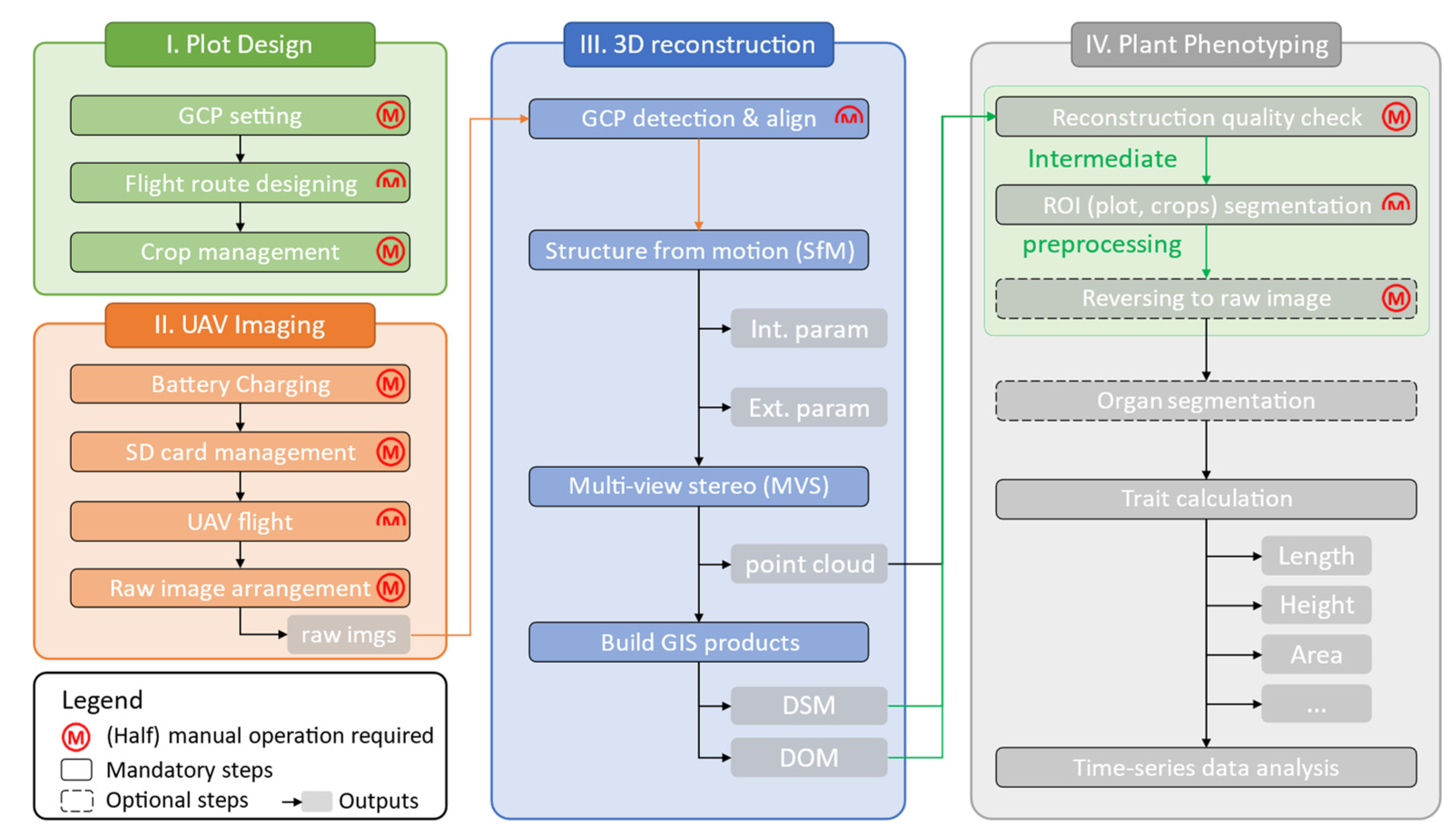
Figure 1. General workflow of UAV-based field plant phenotyping in agriculture. The developed tool focused on decreasing the workload of the intermediate data processing steps (green parts in IV). “Int. param” represents internal parameters (e.g., focal length), and “Ext. param” represents external parameters (e.g., camera position, rotation.). DSM represents the digital surface model, and DOM represents the digital orthomosaic.
Remotesensing 13 02622 g001
Figure 2. Example of reverse-calculating one point from the 3D world coordinates to the 2D pixel coordinates on raw UAV images by a pinhole camera model. (a) Relationship between world coordinate ( O w o r l d ) and camera coordinate ( O c a m ), linked by camera external parameters (position and rotation). (b) Relationship between camera coordinate ( O c a m ) and image coordinate ( O i m g ). (c) Relationship between image coordinate ( O i m g ) and pixel coordinate ( O p i x ). (d) Camera distortion calibration between undistorted images and distorted images caused by the lens.
Remotesensing 13 02622 g002
Figure 3. Cropping results for three randomly chosen ROIs of six fields representing different cultivars or treatments. The digital orthomosaic (DOM) and the point cloud (PCD) used in this figure are from the outputs of Metashape.
Remotesensing 13 02622 g003
Figure 4. Reverse calculation results for six fields. Both Metashape and Pix4D results are used. (a) ROI from Pix4D-produced DOM and (b) ROI from MetaShape-produced DOM. (cf) Randomly selected examples of ROIs on four raw UAV images. The Pix4D lines could be covered by the blue Metashape lines once no significant differences were observed.
Remotesensing 13 02622 g004
Figure 5. Transformation accuracy examination results. Three plots with different lotus leaf densities and heights were selected. All the expected ROI transformation positions were marked manually on raw images using LabelMe annotation software. The distance is the Euclidean pixel distance from the reversed region of interest (ROI) center to the photo center. The distribution of each pixel point height is shown in the blue area, the height of the ROI (solid red lines) is the mean value of all the pixel points smaller than the 5th percentile threshold, and the height of the plot edge (blue broken lines) is the mean value of random 10 points picked from QGIS on the DSM.
Remotesensing 13 02622 g005
Figure 6. Effects of the ROI position and ROI height on the transformation. (a) Three different height choices of ROIs (5th percentile, mean, 95th percentile) by point cloud display, and (b,c) two different ROI positions on the raw images and related ROI transformation results.
Remotesensing 13 02622 g006
Figure 7. Distribution of the transformation accuracy indicators for all 112 lotus plots. For each plot, only ROI-centered raw images (minimum Euclidean distance between ROI center and raw image center) were selected and the references manually marked.
Remotesensing 13 02622 g007
Figure 8. Potential usage of reverse calculation for individual-level training data annotation and augmentation in deep learning. The DOM file of dataset 4 (Orchard) was loaded into LabelMe directly, 6 rectangle annotations (2 for each species) were made, and the annotation JSON file was saved (left-corner screenshot). Reverse calculation was performed on all annotation rectangles for all raw images. “div” means the distance from the annotation center to the image center; smaller is closer.
Remotesensing 13 02622 g008
Figure 9. Potential usage of reverse calculation for organ-level training data annotation and augmentation in deep learning. The DOM file of dataset 5 (lotus) was split into several 500   px × 500   px grids, and the grid “x6-y7” was marked with 6 annotation rectangles for flowers by LabelMe. Reverse calculation was performed on all annotation rectangles for all raw images. “div” means the distance from the annotation center to the image center; smaller is closer.
Remotesensing 13 02622 g009
Table 1. Trial field and image acquisition information.
DatasetCropField LocationFlight Date (yy/mm/dd)UAV ModelCameraModelFlight Height (m)Image Num.Size of Images (px)
1SoybeanTanashi 119/08/07DJI Inspire 1FC550302024608 × 3456
2Sugar beetMemuro 218/06/26DJI Phantom 4 v1FC6310301205472 × 3648
3WheatTanashi19/03/14DJI Inspire 1FC550301384608 × 3456
4OrchardTanashi20/08/06DJI Phantom 4 v2FC6310S501195472 × 3648
5LotusTanashi17/05/31DJI Inspire 1FC550301424608 × 3456
6MaizeTanashi19/07/29DJI Inspire 1FC550301384608 × 3456
1 Nishi-Tokyo, Japan; 2 Hokkaido, Japan.
Publisher’s Note: MDPI stays neutral with regard to jurisdictional claims in published maps and institutional affiliations.