Abstract
Wetlands are important ecosystems that are linked to climate change mitigation. As 25% of global wetlands are located in Canada, accurate and up-to-date wetland classification is of high importance, nationally and internationally. The advent of deep learning techniques has revolutionized the current use of machine learning algorithms to classify complex environments, specifically in remote sensing. In this paper, we explore the potential and possible limitations to be overcome regarding the use of ensemble deep learning techniques for complex wetland classification and discusses the potential and limitation of various solo convolutional neural networks (CNNs), including DenseNet, GoogLeNet, ShuffleNet, MobileNet, Xception, Inception-ResNet, ResNet18, and ResNet101 in three different study areas located in Newfoundland and Labrador, Canada (i.e., Avalon, Gros Morne, and Grand Falls). Moreover, to improve the classification accuracies of wetland classes of bog, fen, marsh, swamp, and shallow water, the results of the three best CNNs in each study area is fused using three supervised classifiers of random forest (RF), bagged tree (BTree), Bayesian optimized tree (BOT), and one unsupervised majority voting classifier. The results suggest that the ensemble models, in particular BTree, have a valuable role to play in the classification of wetland classes of bog, fen, marsh, swamp, and shallow water. The ensemble CNNs show an improvement of 9.63–19.04% in terms of mean producer’s accuracy compared to the solo CNNs, to recognize wetland classes in three different study areas. This research indicates a promising potential for integrating ensemble-based learning and deep learning for operational large area land cover, particularly complex wetland type classification.
1. Introduction
Wetlands cover 3% to 8% of the Earth’s land surface and are amongst the most valuable ecosystems across the world [1]. Wetlands make invaluable contributions to the maintenance and quality of life for nature and humanity. Since the plants, bacteria, and animals in wetlands filter the water, trapping nutrients like phosphorus, one of the main reasons for harmful algae blooms in water bodies, wetlands are usually referred to as the kidneys of the earth [2,3]. Carbon sequestration, food security, water storage, as well as flood and shoreline protection are only some of the services provided by wetlands [4,5]. Also, they provide critical habitat that supports plant and animal biodiversity [6,7]. Despite these benefits, agricultural activities, industrialization, urbanization, and climate change are destroying these ecosystems at an alarming rate [1]. As such, systematic monitoring of these threatened ecosystems is needed for their preservation.
Remote sensing is preferred to conventional labor-intensive methods, such as field surveying, as it provides a relatively cost-effective large-scale methodology for monitoring wetlands [8,9,10]. Large-scale monitoring of wetland areas can be achieved through the use of optical and synthetic aperture radar (SAR) remote sensing using state-of-the-art machine learning (ML) algorithms in cloud computing platforms [11,12]. However, large-scale wetland mapping is considered a challenging task relative to conventional land use land cover (LULC) classification. This is largely due to difficulties that are a result of the inherent biological and ecological characteristics of wetland ecosystems. For instance, wetlands are not unified by a common type of vegetation or land cover [1], but are instead unified based on the presence of water below the vegetation canopy or at or near the surface of the ground. Additionally, the complexity of wetlands in terms of vegetation composition, shape, and position in the landscape means that satellite sensors’ capacity for their classification is often insufficient. As a result, several conventional and advanced ML models have been developed and tested for wetland classification [13,14].
Conventional ML classification consists of two different components, feature extraction, and classification [15,16,17,18]. In the feature extraction stage, spatial, spectral, and temporal Earth observation (EO) data are transformed into feature vectors. In the classifier stage, those extracted features are used to train and deploy the ML model [19]. Recently, deep learning (DL) has been frequently employed in remote sensing image classification [12,20,21,22]. DL algorithms learn from representation rather than an empirical feature design. The representations of internal features are automatically learned, and thus these methods are considered highly efficient approaches for image classification [19]. Among the deep learning algorithms, convolutional neural networks (CNN), inspired by biological processes, are frequently applied for remote sensing image classification and has achieved very high accurate results in high-dimensional and complex environments [11,22,23,24,25,26,27]. The main reason for this superiority is that DL models usually can find more generalized patterns compared to shallow ML models [28,29]. The superior performance of deep learning methods can also be attributed to their ability to include feature extraction in the optimization process [30]. It should be noted that, although DL models achieve remarkable accuracies, they require more training data as well as advanced computing resources compared to ML methods [31]. The input of a CNN model is a feature map (i.e., a patch of image) rather than a single pixel used in traditional classification methods. CNN can then learn the boundaries, textural, and topological characteristics of those patches [30]. An advantage of CNN is described as its translational invariance, which allows shifted or distorted objects to be discovered. Generally, CNN has two layers, including convolutional and subsampling layers (i.e., pooling layers). First, through multiple groups of convolutional layers, the characteristics of different objects are recognized. Then, the pooling layer is used for downscaling the feature maps to reduce computation cost. Finally, a flattening layer transfers the feature maps into a one-dimensional vector where they are categorized into several classes [28,32,33].
In this study, we discuss the potential and possible limitations of the DL model and based on that we compare the results of solo versus ensemble deep learning models for complex wetland classification. We also discuss the potential and limitation of various CNNs, including DenseNet, GoogLeNet, ShuffleNet, MobileNet, Xception, Inception-ResNet, ResNet18, and ResNet101 in three different study areas located in Newfoundland and Labrador, Canada (i.e., Avalon, Gros Morne, and Grand Falls). To do that, we examine the ability of a proposed ensemble CNN model with two different classification strategies: (1) employing majority voting in the last layer; (2) applying a machine learning classifier, including random forest (RF), bagged tree (BTree), and Bayesian optimized tree (BOT) in the last layer. To the best of our knowledge, this is the first attempt to investigate the ability of ensemble CNNs for wetland classification using multispectral satellite imagery. Therefore, this study contributes to the support of the use of the state-of-the-art deep learning model for wetland mapping using high-resolution remote sensing data.
2. The Study Area and Training Data
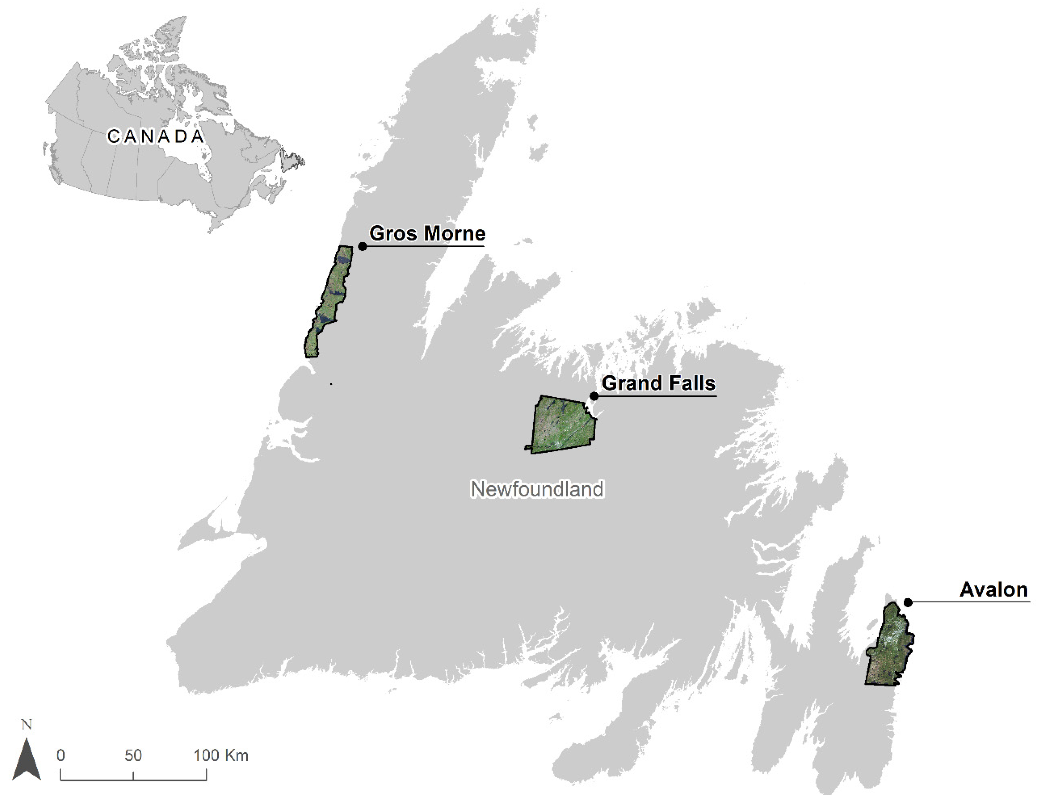
In this study, three different study areas are used, located in and around the region of Avalon, the town of Grand Falls-Windsor, and Gros Morne National Park, on the island of Newfoundland in Canada, as presented in Figure 1. Within the study areas, the dominant land cover is highly productive coniferous forests and vast peatlands [34]. Essential wetland habitat for waterfowl for nesting and raising of young and other natural ecosystems are found within these study areas. All wetland classes (including bog, fen, marsh, swamp, and shallow water) are located within the study areas’ borders. The most dominant wetland classes are bog and fen, broadly referred to as peatlands. Ground-truth data were collected by a team of ecologists and wetland specialists in the summers of 2015, 2016, and 2017. Before field visitation, potential wetland sites were identified based on the visual interpretation of RapidEye and Google Earth imagery. Then, sites were visited in the field where wetlands were classified as bog, fen, swamp, marsh, or shallow water classes based on the Canadian Wetland Classification System (CWCS), a wetland classification standard for the country. Dominant vegetation groups, the presence of certain plant species, hydrology, and landscape position were considered when assigning a wetland a class.
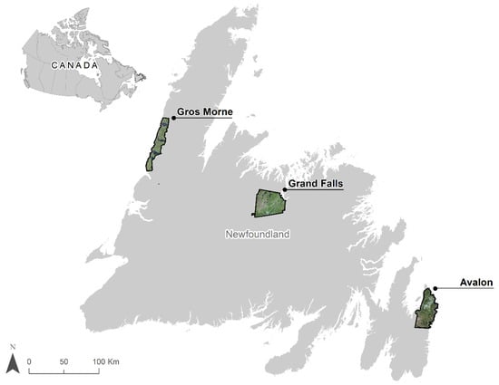
Figure 1.
The study areas located on the Island of Newfoundland in Canada.
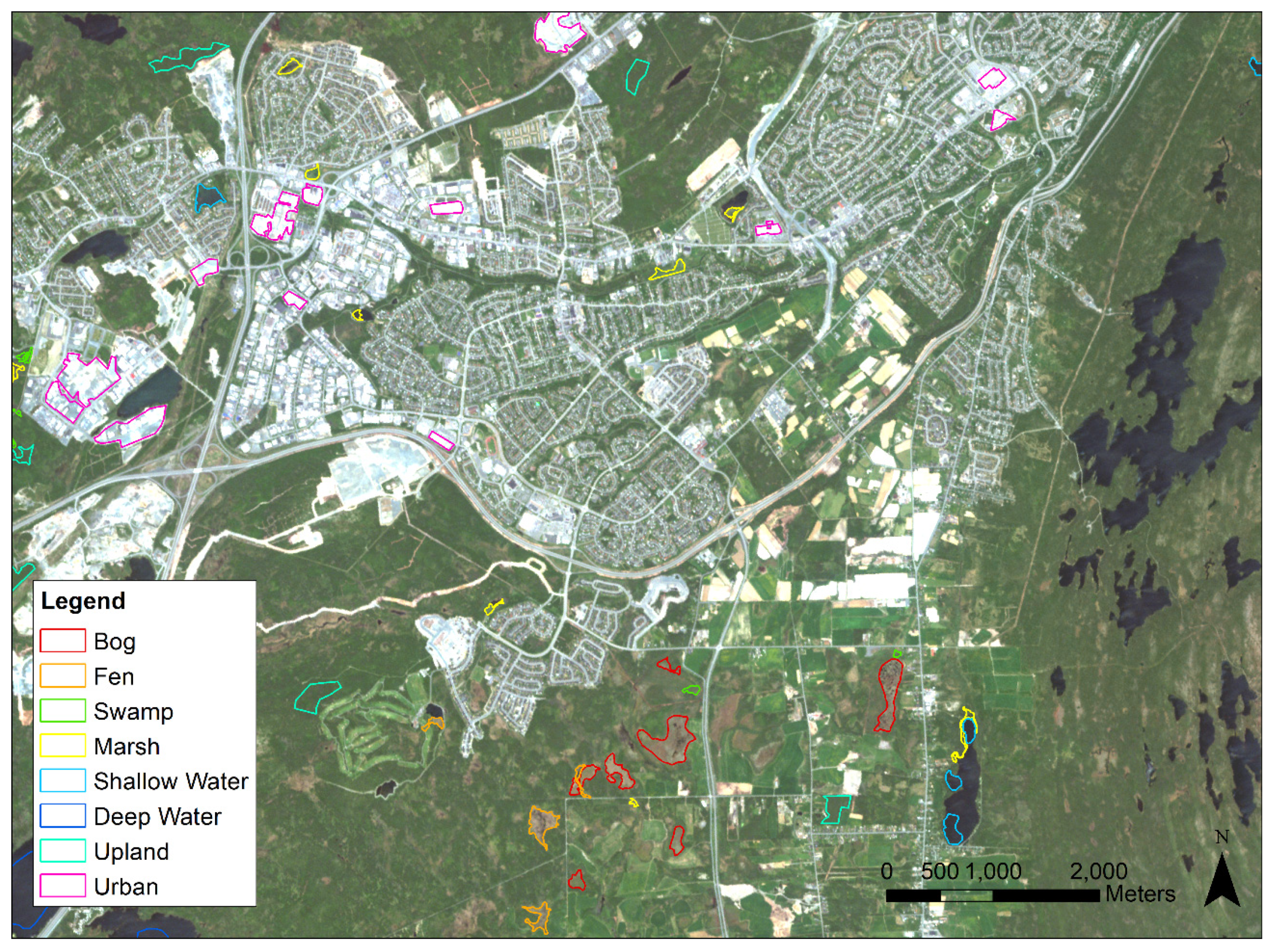
Global positioning system (GPS) points, along with notes and photos, were taken in the field for use as a guide for the delineation of polygons representing the wetlands visited. Refer to Figure 2 for examples of the delineated polygons. To improve the accuracy of delineation, multi-season, and multi-year, Google Earth imagery is used as ancillary data. See Table 1 for the number of training and test data (i.e., pixels).
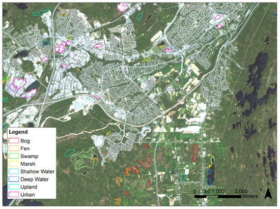
Figure 2.
A sample of ground-truthed wetlands in the Avalon.

Table 1.
The number of training and test data.
In this study, five bands of blue (440–510 nm), green (520–590 nm), red (630–685 nm), red edge (690–730 nm), and near-infrared (760–850 nm) of RapidEye imageries are used. In particular, two level 3a RapidEye imagery with a spatial resolution of five meter, collected on 18 June and 22 October 2015, were used for wetland mapping. To improve the wetland classification accuracy, three spectral indices, namely red edge normalized difference vegetation index (RENDVI), ratio-vegetation index (RVI), and green NDVI (GNDVI), are utilized as well (Table 2).

Table 2.
The spectral bands and indices used in this research.
It is worth noting that for the CNN model results evaluation, we used the pixel-based comparison of the ground truth and predicted classes in each study area of the Avalon, Grand Falls, and Gros Morne. In this study, different polygons were selected for training and test data to avoid the autocorrelation between the datasets. Reference polygons, sorted by size, were alternatingly assigned to testing and training datasets for each class. The reason was to ensure that both the training and test data had a comparable number of pixels for each class. Due to the limited number of data and the wide variation of size within each wetland class (some large, some small), random assignment of polygons training and test groups may result in the group having highly uneven pixel numbers. This method may result in lower accuracy; however, in comparison to random sampling, the confidence level of the achieved results will be high.
3. Methods
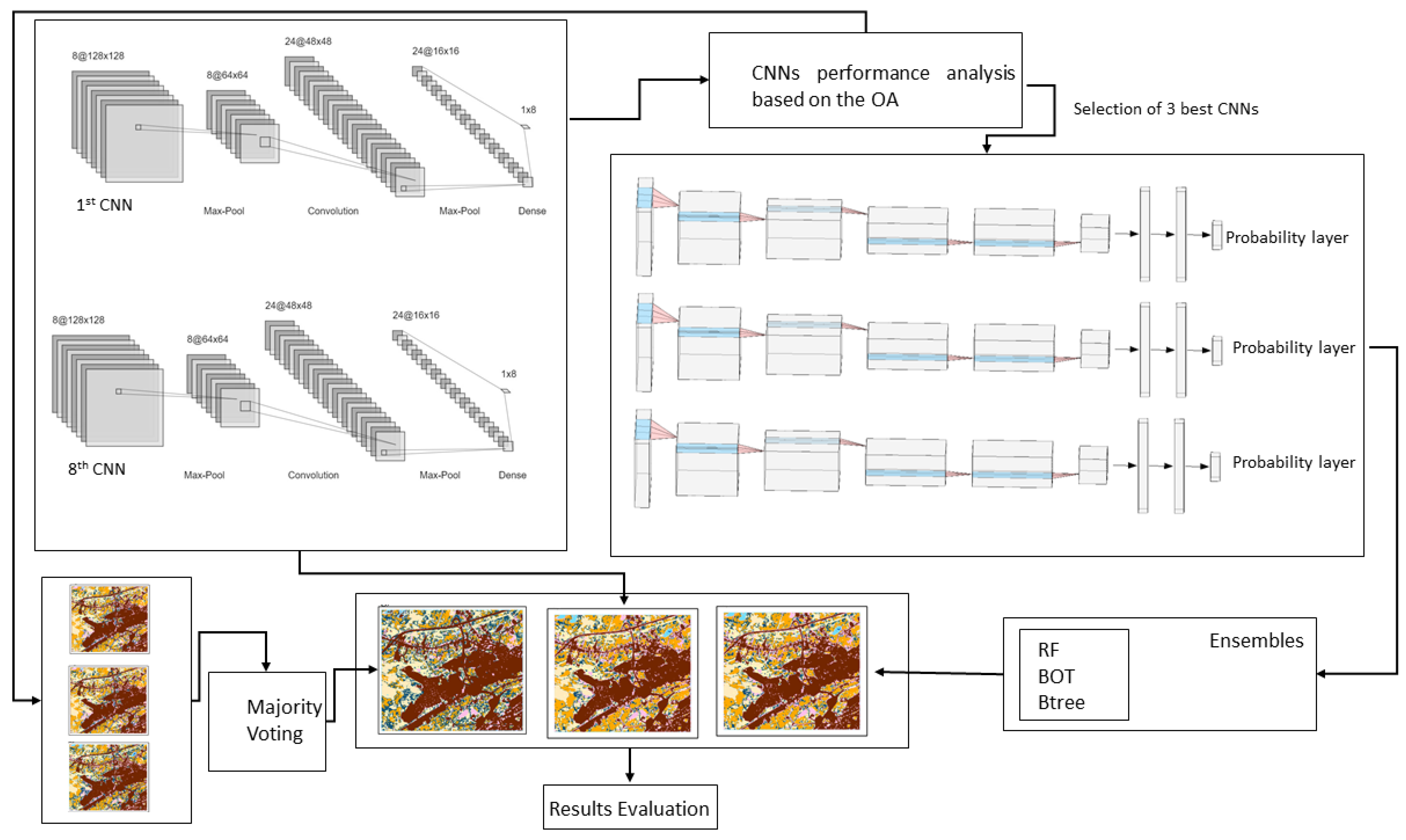
The flowchart of the proposed ensemble modeling for complex wetland classification is shown in Figure 3. As seen, the proposed framework can be summarized in four steps: (1) evaluate the performance of each solo CNN model for wetland classification using multi-spectral RapidEye satellite data, (2) select the best three CNN models based on accuracy assessments indices, (3) apply ensemble modeling using two different strategies of majority voting and employing supervised machine learning models (i.e., RF, BTree, and BOT), (4) Evaluate of results of solo versus ensemble CNN models for wetland classification. In this section, the processing steps are explained in more detail.
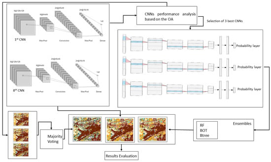
Figure 3.
The framework of the proposed ensemble deep learning model for wetland classification.
3.1. Convolutional Neural Networks (CNNs)
CNNs are the most popular deep learning techniques and have recently attracted a substantial amount of attention in the remote sensing community. These supervised non-linear models can automatically extract important features without any human supervision. Specifically, CNNs are multi-layer interconnected neural networks that hierarchically extract powerful low-, intermediate-, and high-level features. In each layer (l), these features are extracted based on the weights (W) and biases (B) of the previous layers, which are updated in each iteration as follows (Equations (1) and (2)):
where λ, x, and n denote a regularization parameter, learning rate, the total number of training samples, and m, t, and C are momentum, updating step, and cost function, respectively. According to the dataset, the regularizing parameter (λ), learning rate (x), momentum (m) will be tuned to achieve optimum performance.
In particular, the optimum λ prevents overfitting of the data, the learning rate controls the training time, and momentum can help to converge the data. A typical CNN framework consists of three different layers, namely a convolutional layer, a pooling layer, and a fully connected layer, which are described in more detail below.
Convolutional layer: The main body of a CNN architecture is the convolutional layer, which contains several filters sliding across the image. General speaking, convolution is a mathematical operation that merges two different sources of information (i.e., input image and filter) given by:
where y is the feature map and x, f, and n are the input image, filter, and the number of pixels in the image, respectively.
Pooling layer: This layer is usually implemented after the convolution layer to reduce the dimensionality and number of parameters. This also helps to reduce training time and to prevent overfitting. The down-sampling layer is another term that has been used for the pooling layer because it spatially down-samples each feature map. Although several functions such as average pooling or even L2-norm pooling can be used as a pooling layer, most studies use max-pooling operation (with filters of size 2 × 2 and stride 2).
Fully connected layer: Similar to typical neural networks (NNs), the neurons in this layer have full connections to all of the activations in the previous layer. The overfitting problem mostly occurs in the fully connected layer because it contains a higher number of parameters. Dropout is a regularization solution in neural networks that reduces interdependent learning amongst neurons in fully connected layers. The classification layer is the last layer of a CNN model. The SoftMax function is the most commonly used classification layer that outputs a vector representing the probability distributions of the potential classes.
3.2. Models
3.2.1. GoogLeNet (GN)
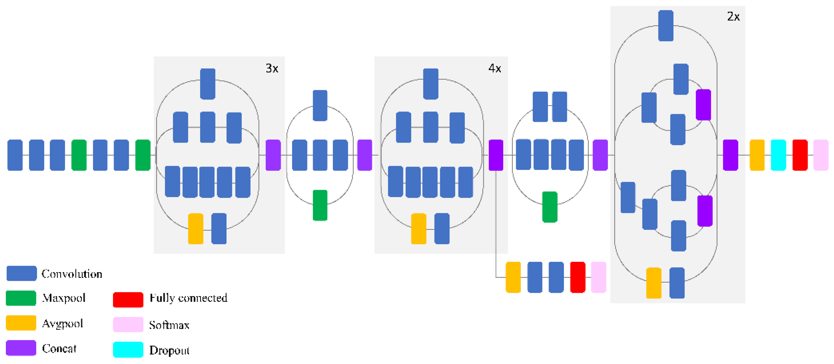
GN has been proposed by [36] for computer vision applications, such as image classification and object recognition. In this CNN algorithm, an innovative approach called the Inception module was introduced. There are nine operations of convolution and pooling layers in the structure of the GN method. Besides that, to reduce the cost of computation, a one-by-one window size was suggested for the convolutional layers at the end of its structure. As a consequence of using a one-by-one window size, input sizes of the convolution layers are decreased, resulting in a faster and more efficient computation (Figure 4). The GN algorithm was proposed to solve two issues of conventional CNNs. Notably, there are too many parameters in the deep CNN model to be estimated. A high number of parameters, in this case, would result in overfitting. Moreover, having too many layers in the CNN model means increasing the computation cost. By replacing the fully connected layer with sparse layers, the GN algorithm solved these issues.
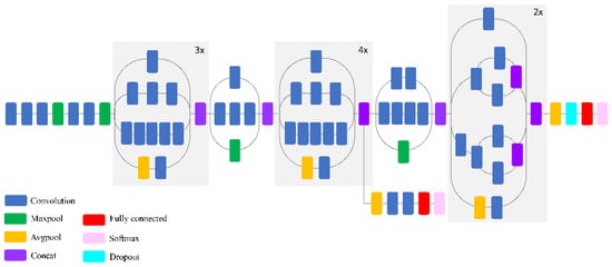
Figure 4.
Schematic diagram of the InceptionV3 model (compressed view) [11].
3.2.2. MobileNet
Given the limited hardware and computation restrictions of mobile devices, image recognition MobileNet architectures were introduced and are considered to be efficiently designed CNNs [37]. The highly efficient MobileNet-224 was proposed by [38], which uses depth-wise separable convolutions. In MobileNet-224, for each input feature map separately, three by three convolution stacks are used, which are considered highly efficient (Figure 5).
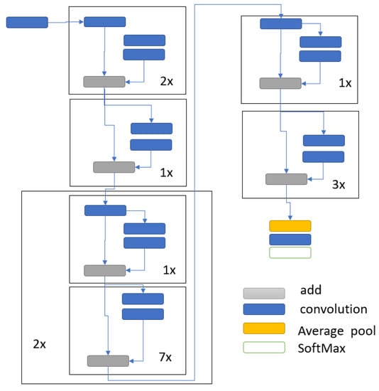
Figure 5.
Schematic diagram of the MobileNet (compressed view).
3.2.3. Xception
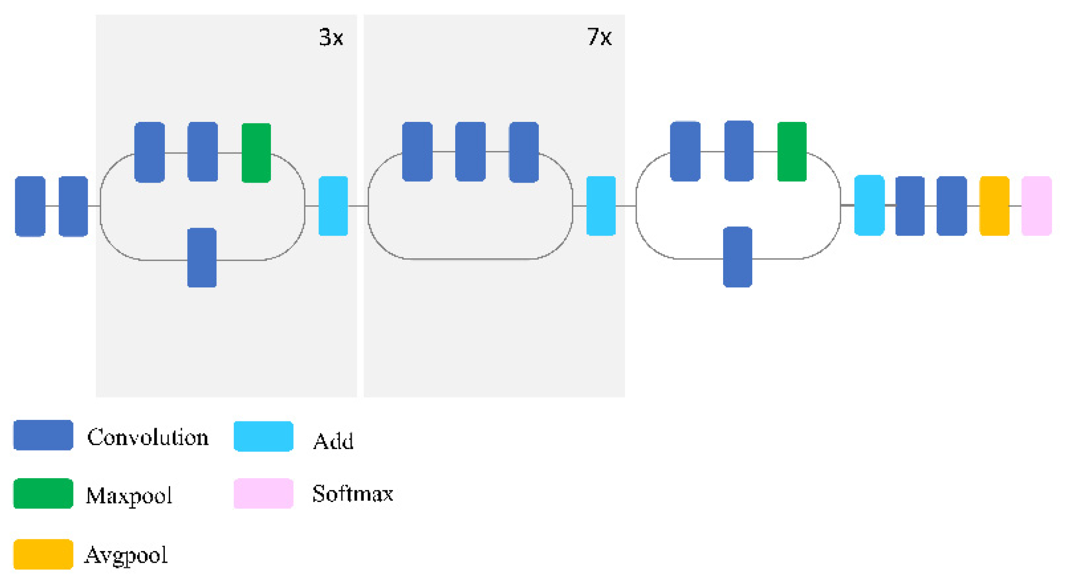
Xception is considered to be a family member of Inception networks proposed by [39]. Inception models introduced complex building block structures, bottleneck design, batch normalization, as well as space and depth factorization. The Xception networks implement the use of factorization in its structure, where for feature extraction, it uses depth-wise separable convolutions (Figure 6). For each output channel, without using any non-linear activation function, the Xception uses a point-wise convolution of one-by-one with an adjacent three by three depth-wise convolution [37].

Figure 6.
Schematic diagram of the Xception model (compressed view) [11].
3.2.4. ShuffleNet
To decrease computation cost, point-wise group convolution and channel shuffle were utilized in the ShuffleNet [40]. Particularly, this model maintains the accuracy level of very deep CNN algorithms while having efficient computation costs. It is worth noting that the computation complexity and target platform, which define the computation budget, were a major consideration in the creation of the ShuffleNet method. As a result, under the equal setting with the ResNet and ResNetX [41], the ShuffleNet model has lower complexity (Figure 7). Also, with accuracy comparable to AlexNet, the ShuffleNet was almost thirteen times faster on a mobile device.
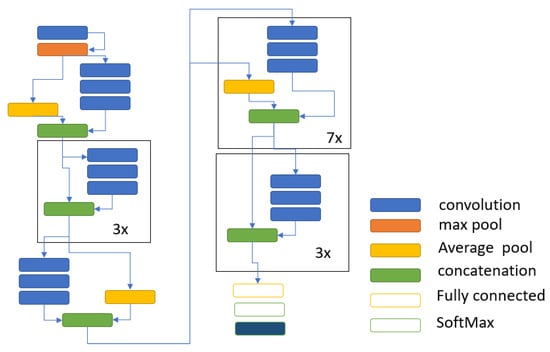
Figure 7.
Schematic diagram of the ShuffleNet model (compressed view).
3.2.5. ResNet
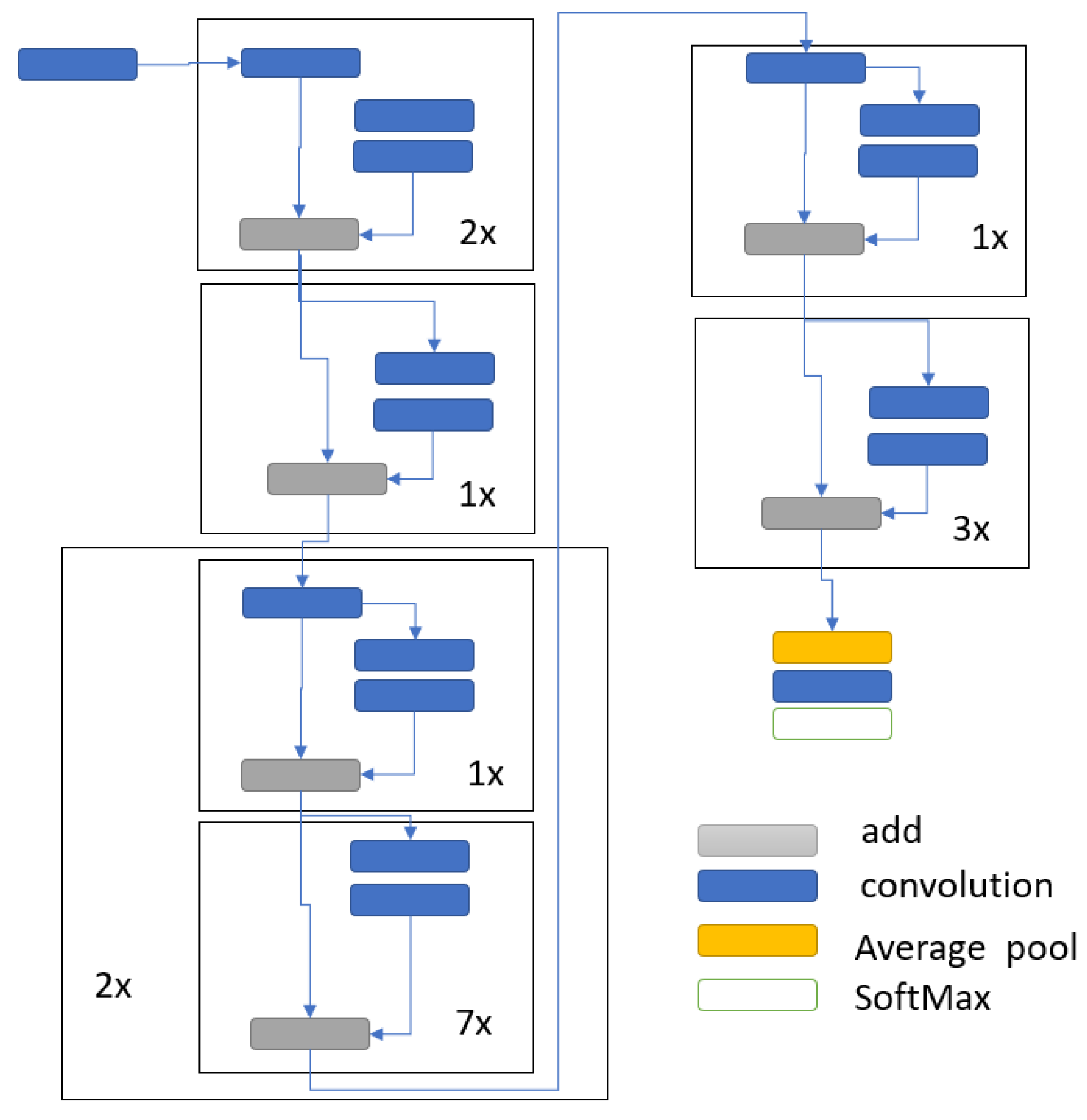
The bottleneck structure was proposed in the ResNet method, achieving an impressively high accuracy [41,42]. In ResNet, instead of learning unreferenced functions, layers are created as the residual learning functions (Figure 8). By increasing the depth of the network [43], residual networks of the ResNet were easier to optimize, achieving higher accuracy. Moreover, the degradation problem of very deep CNNs was solved by the deep residual learning framework in the ResNet method. It is worth noting that, in conventional CNNs, degradation occurs as depth increases where the accuracy will first be saturated and then degraded.

Figure 8.
Schematic diagram of the ResNet model (compressed view) [11].
3.2.6. Inception-ResNet
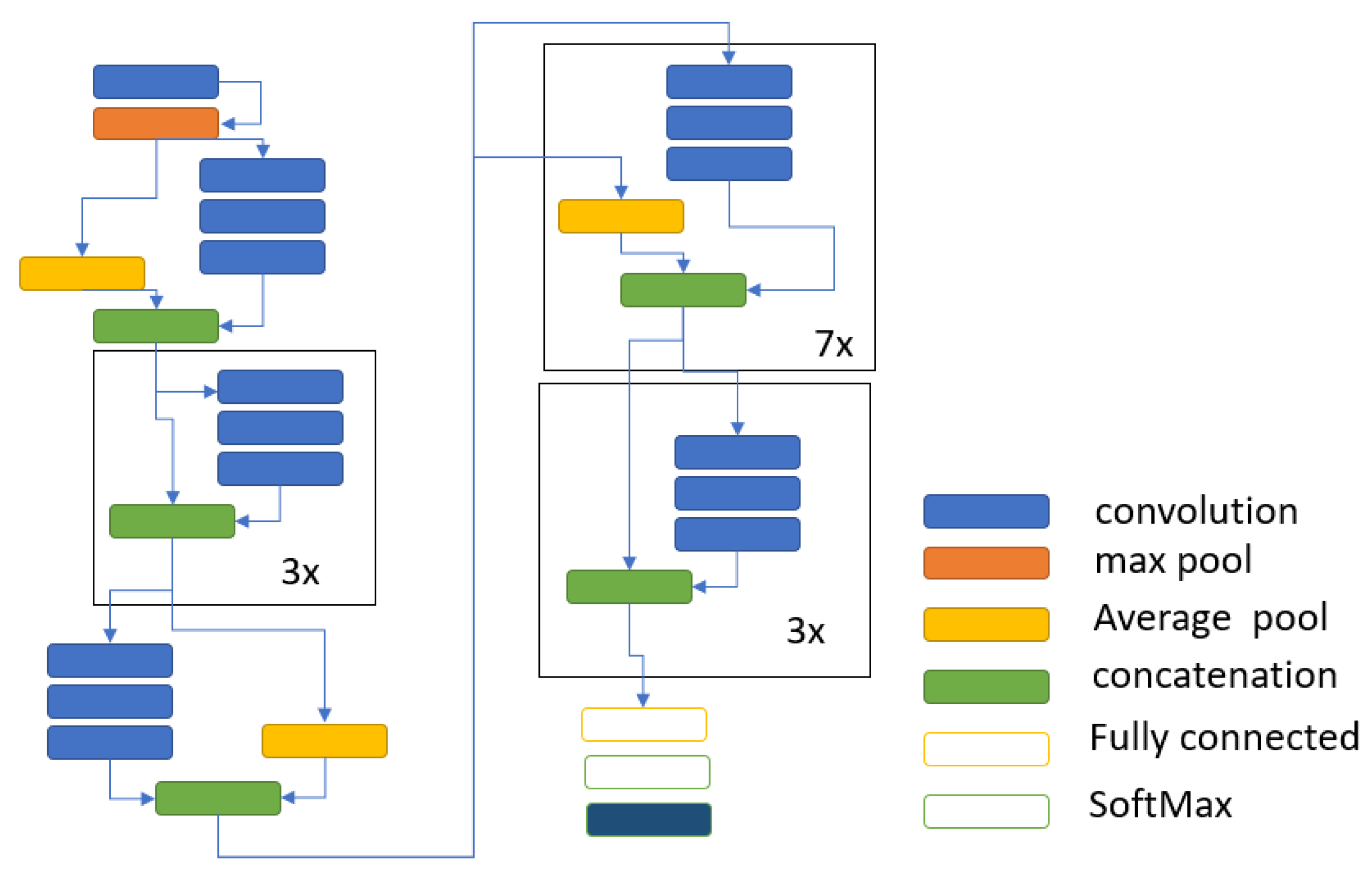
Inception-ResNet is a combined version of Inception and ResNet modules developed by [44]. Inception-ResNet utilizes both characteristics of Inception and ResNet networks. This model has a similar architecture to Inception while benefiting from the bottleneck structure, batch normalization, and residual connections of ResNet [37]. It is deeper than the ResNet and Inception modules, where, unlike its ancestors, it does not require any auxiliary classifiers. Moreover, with fewer parameters, the Inception-ResNet has equal or better results than the ResNet and Inception networks (Figure 9).

Figure 9.
Schematic diagram of the Inception-ResNet model (compressed view) [11].
3.2.7. DenseNet
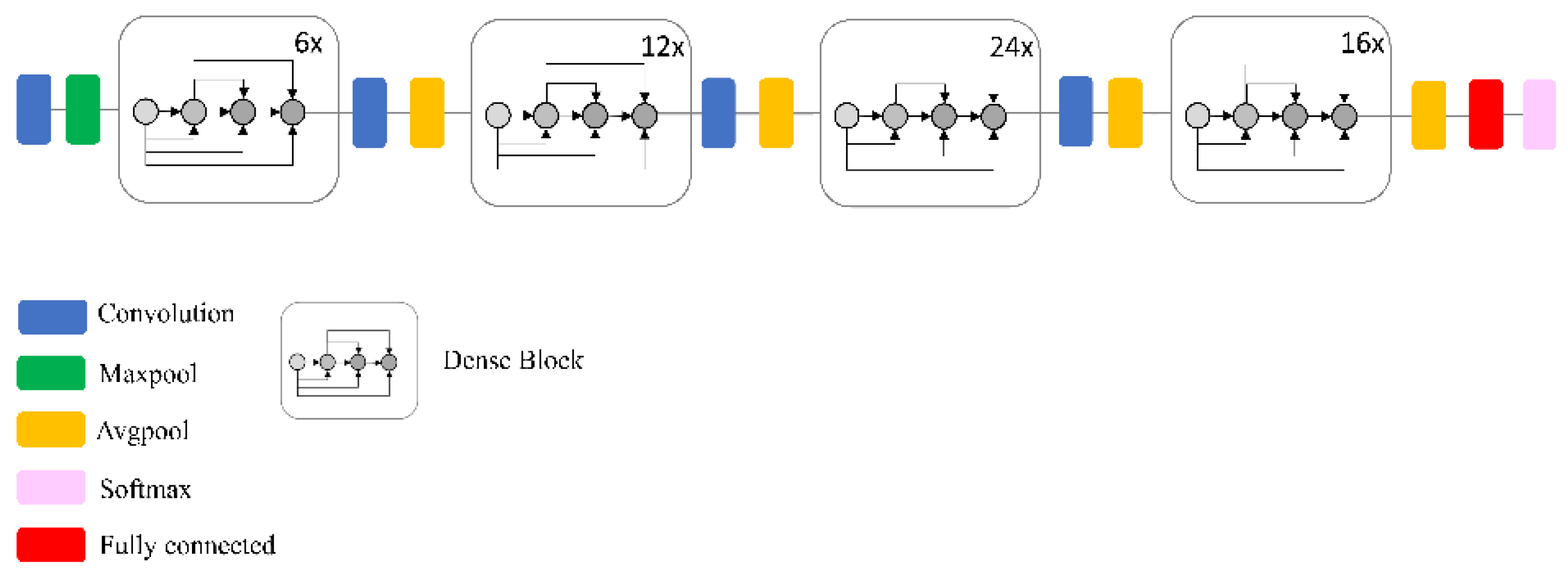
DenseNet, proposed by [45] is amongst those ResNet networks that use intensively residual connections. DenseNet, as its name suggests, has a densely connected building block where each convolutional layer uses the output of previous convolutions and all inputs inside its block using several residual networks. Layers in DenseNet are merged by the concatenation layer, which results in a very deep feature map. Like other Resnet networks, DenseNet uses a bottleneck design to reduce its depth [37] (Figure 10).

Figure 10.
Schematic diagram of the DenseNet model (compressed view) [11].
3.3. Ensemble CNN Models
In this study, we trained several well-known CNN models where each model assigns different labels to each region of the image. Due to classification errors resulting from insufficient or poor training, different models will sometimes assign different labels to the same image patch. This classification error can be minimized through an ensemble model, where the outputs of different trained models are ensembled to minimize error. In this section, we introduce two main ensemble techniques that we used to enhance the performance of the trained solo CNN models.
3.3.1. Majority Voting Algorithm
As described by Equation (4), majority voting is the most simple ensemble technique where for each image patch, the label produced by the majority of the models is assigned to that patch:
where mode(.) is the “mode” or majority function, is the label produced by the mth CNN model, M is the number of the CNN models, and is the final label assigned to the image patch. It should be noted that majority voting is an unsupervised ensemble approach as it does not require an additional training step for training.
3.3.2. Machine Learning-Based Approach
To improve the classification results of the solo CNN networks, the probabilities produced by the softmax layer of a CNN model can be used for another phase of training. The probabilities generated by the CNN models can be classified using well-known machine learning classification techniques, such as Support Vector Machine (SVM), k-nearest neighbors (KNN), or decision tree-based algorithms. In this paper, we employ supervised classifiers of RF, BTree, and BOT to classify these features. In contrast to the majority voting method, this approach is a supervised method as it requires an additional training step. The trained CNNs are evaluated in terms of the overall accuracy and producer’s accuracy based on the test data, which are derived from different sets of polygons and are unseen for the model during hyper-parameters tuning and the training phase (Equations (5) and (6)). It is worth noting that the test data are evaluated individually for each of the three study regions:
4. Results and Discussion
This research phase consisted of results evaluation designed to assess if solo CNNs can detect complex wetland classes to an acceptable accuracy. To do so, the overall and producer’s accuracies were used to evaluate the capability of different models for identification of the wetland classes (i.e., bog, fen, marsh, swamp, and shallow water) as well as non-wetland classes (i.e., urban, upland, and deep water).
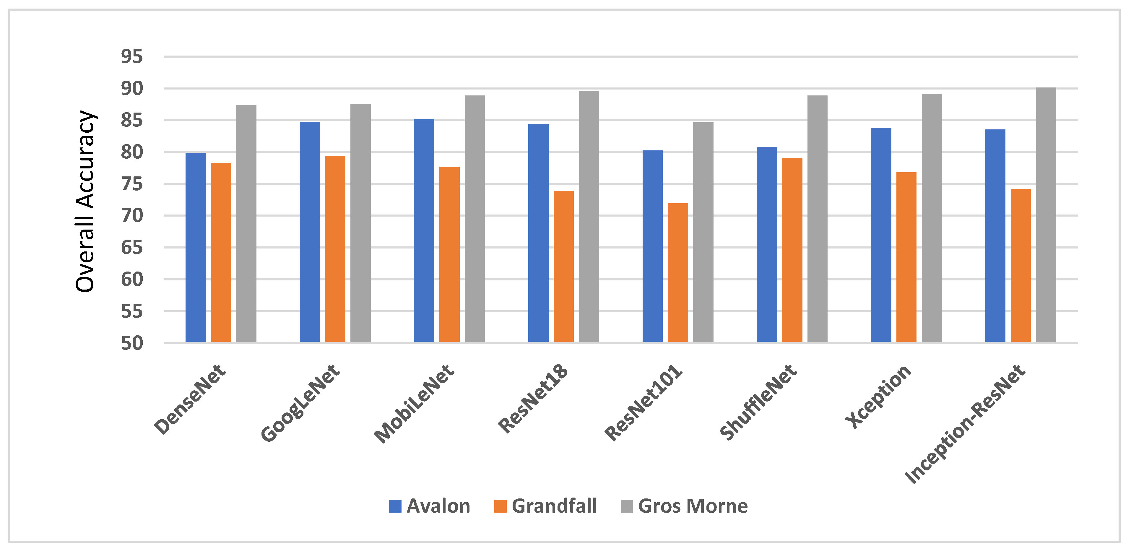
The overall accuracy values for the solo CNNs from a comparison of reference and predicted classes are summarized in Figure 11. Comparisons were made for three different study areas of Avalon, Grand Falls, and Gros Morne. The overall accuracies indicated a strong level of agreement between the reference and predicted classes of wetland in the Gros Morne region (OA = 84.63–90.14%), followed by the Avalon area (OA = 79.86–85.16%) and the Grand Falls (OA = 71.93–79.34%). Generally, the lower level of accuracy of the Grand Falls can be explained by the lower numbers of training data for non-wetlands and the high level of complexity in wetlands in this study area.
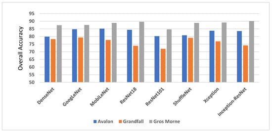
Figure 11.
Results of CNNs for the test data sets of the three study areas (in percent).
To evaluate the time cost of different CNN models, their training time was assessed, as shown in Figure 12. The Inception-ResNet and DenseNet models required the longest time for training at 1392 and 1181 min, respectively. In contrast, the ResNet18 model required the least amount of time for training at 73 min. The comparison revealed the advantage of shallow CNNs compared to deep CNNs in terms of overall accuracy and time. This is because there are a higher number of parameters to be fine-tuned in the deeper CNNs, which increases the time and computational costs. Also, these CNN models with a high number of layers require larger training samples to achieve their full potential, which may result in a lower level of accuracy. It is worth highlighting that the experiments were done with an Intel processor (i.e., i5-6200U Central Processing Unit (CPU) of 2.30 GHz) and an 8 GB Random Access Memory (RAM) operating on 64-bit Windows 10.
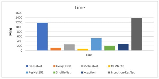
Figure 12.
The time required to train the CNN networks (the total value is equal to 4036 min).
We also evaluated the efficiency of different solo CNN models in each study area in terms of producer’s accuracy, as described in more detail in the following subsections.
4.1. Avalon Study Area
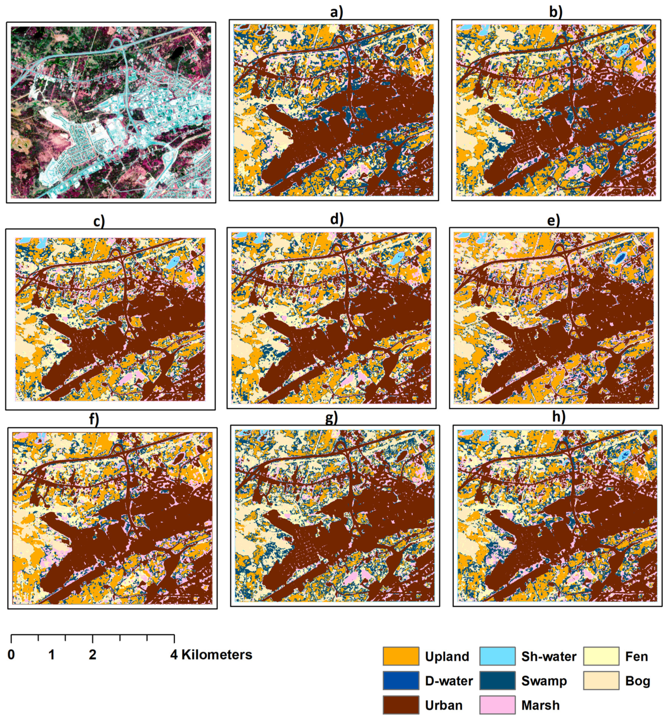
A part of the Avalon study area with approximately 4.2 km by 4.9 km was used for the classification mapping (Figure 13). As seen in Table 3, all the solo CNN models have demonstrated poor performances in identifying fen, marsh, and swamp wetland classes. There were few training data for fen, marsh, and swamp wetland classes in this study area. Consequently, the classification results of the CNN models in terms of producer’s accuracy were less than 60%. It is worth mentioning that wetland classes do not have a clear-cut boundary (e.g., wetlands have irregular boundary shapes), and some of these classes may have similar vegetation types and structures, resulting in similar spectral reflectance values. For example, the accuracy of fen classification was low and incorrectly classified as bog.
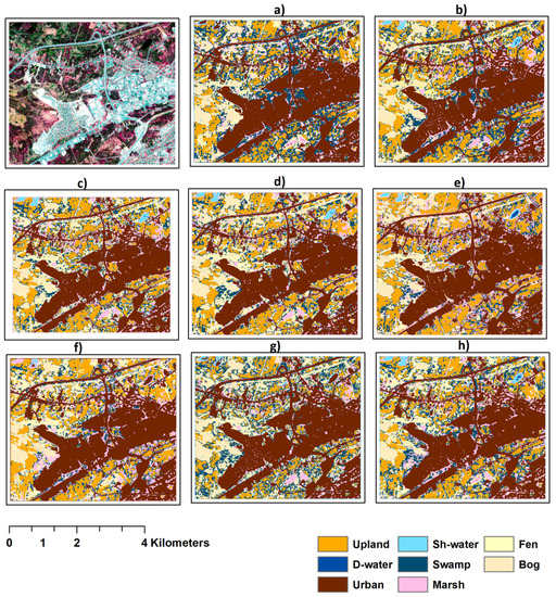
Figure 13.
Map of a part of the Avalon area showing the classification results of the CNN models using (a) DenseNet, (b) GoogLeNet, (c) Inception-ResNet, (d) MobileNet, (e) ResNet101, (f) ResNet18, (g) ShuffleNet, and (h) Xception.

Table 3.
The producer’s accuracy of the CNNs for the Avalon region (in percent).
Additionally, some marsh regions were classified as fen areas. Moreover, most of the swamp areas were recognized as uplands. Generally, these can be explained as a result of the similarity shared between bog, fen, and marsh classes in terms of vegetation pattern (i.e., wet soils, some emergent, and saturated vegetation), as well as the similarity between the swamp and upland forest in terms of tree dominance, in addition to the overall low amount of training data required for training very deep learning models (Figure 13 and Table 3).
In terms of the overall classification accuracy, the MobileNet CNN network with a value of 85.16% had the best classification accuracy in the Avalon, while the least performance was for the CNN network of DenseNet with an overall accuracy of 79.86% (Figure 11).
4.2. Grand Falls Study Area
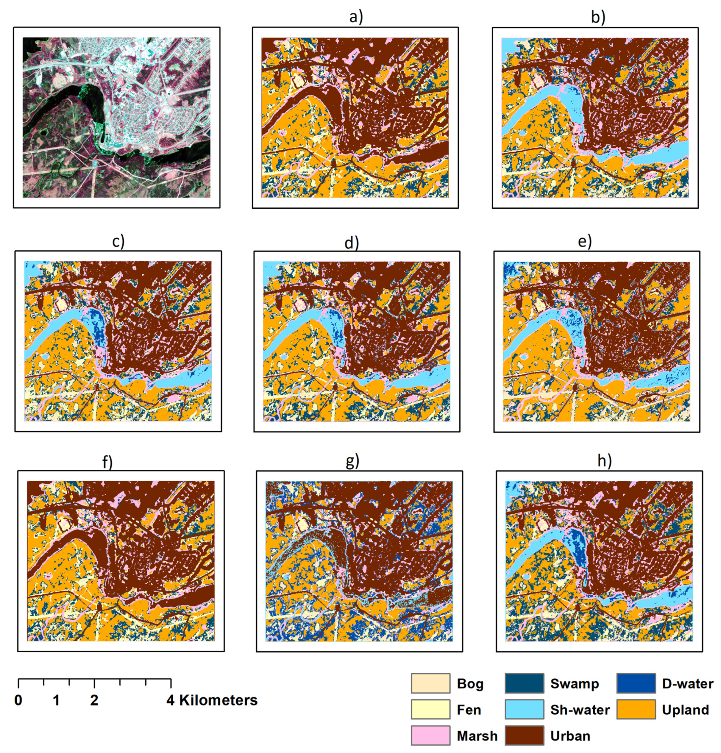
A part of the Grand Falls study area with approximately 4.2 km by 4.9 km is used for the classification mapping (Figure 14). Like the Avalon area, the CNN models had poor performances for distinguishing the bog, fen, and marsh classes, likely due to their spectral similarity and the low amount of training data. In the Grand Falls, most of the swamp areas were incorrectly classified as bog, followed by fen, marsh, and upland classes. Also, shallow water was classified as deep water in some cases, potentially resulting from spectral similarities (Table 4). Results indicated that all CNN models had achieved a high producer’s accuracy for recognizing non-wetland classes of urban and upland. It can be generally explained by their higher number of training data relative to that of wetland training samples.
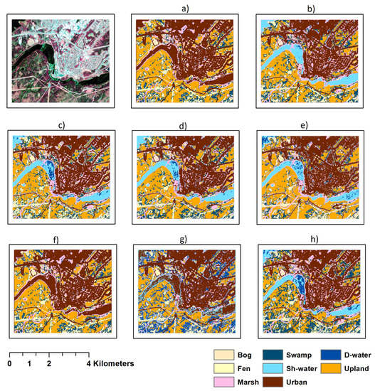
Figure 14.
Map of a part of the Grand Falls area showing the classification results of the CNN models using (a) DenseNet, (b) GoogLeNet, (c) Inception-ResNet, (d) MobileNet, (e) ResNet101, (f) ResNet18, (g) ShuffleNet, and (h) Xception.

Table 4.
The producer’s accuracy of the CNNs for the Grand Falls region (in percent).
The CNN models had a lower producer’s accuracy in the Grand Falls than that of the Avalon and Gros Morne regions due to the relative complexity of this study area. Fen, marsh, and swamp regions were better recognized by the CNN models in this study region than the Avalon. This could be attributed to the higher number of training data in the Grand Falls for the fen and marsh classes relative to the Avalon and Gros Morne regions. However, they demonstrated relatively poor performances on the classification of shallow water class than that of the Avalon.
In addition, as the number of training data for urban, deep water, and upland classes was less in the Grand Falls, the overall accuracy obtained in this area was much less compared to the Avalon and Gros Morne. The CNN networks of GoogLeNet and ShuffleNet, with the overall accuracies of 79.34% and 79.07%, were superior over the other CNN models, while the least overall accuracy belonged to the CNN network of ResNet18 (Table 4 and Figure 11 and Figure 14).
In the Grand Falls with much less training data, CNN networks, including ShuffleNet and GoogLeNet, were superior over the deeper CNN models of Inception-ResNet and ResNet101. It is due to the reason that there are fewer parameters to be fine-tuned in CNN networks of ShuffleNet and GoogLeNet. There were a higher number of training data for wetland classes in the Grand Falls; consequently, the classification accuracy was higher in this study area than the Avalon and Gros Morne. On the other hand, the training data for the non-wetland classes were relatively low in the Grand Falls, resulting in a lower overall accuracy ranging from 73.87% to 79.34% (Figure 11 and Figure 14).
4.3. Gros Morne Study Area
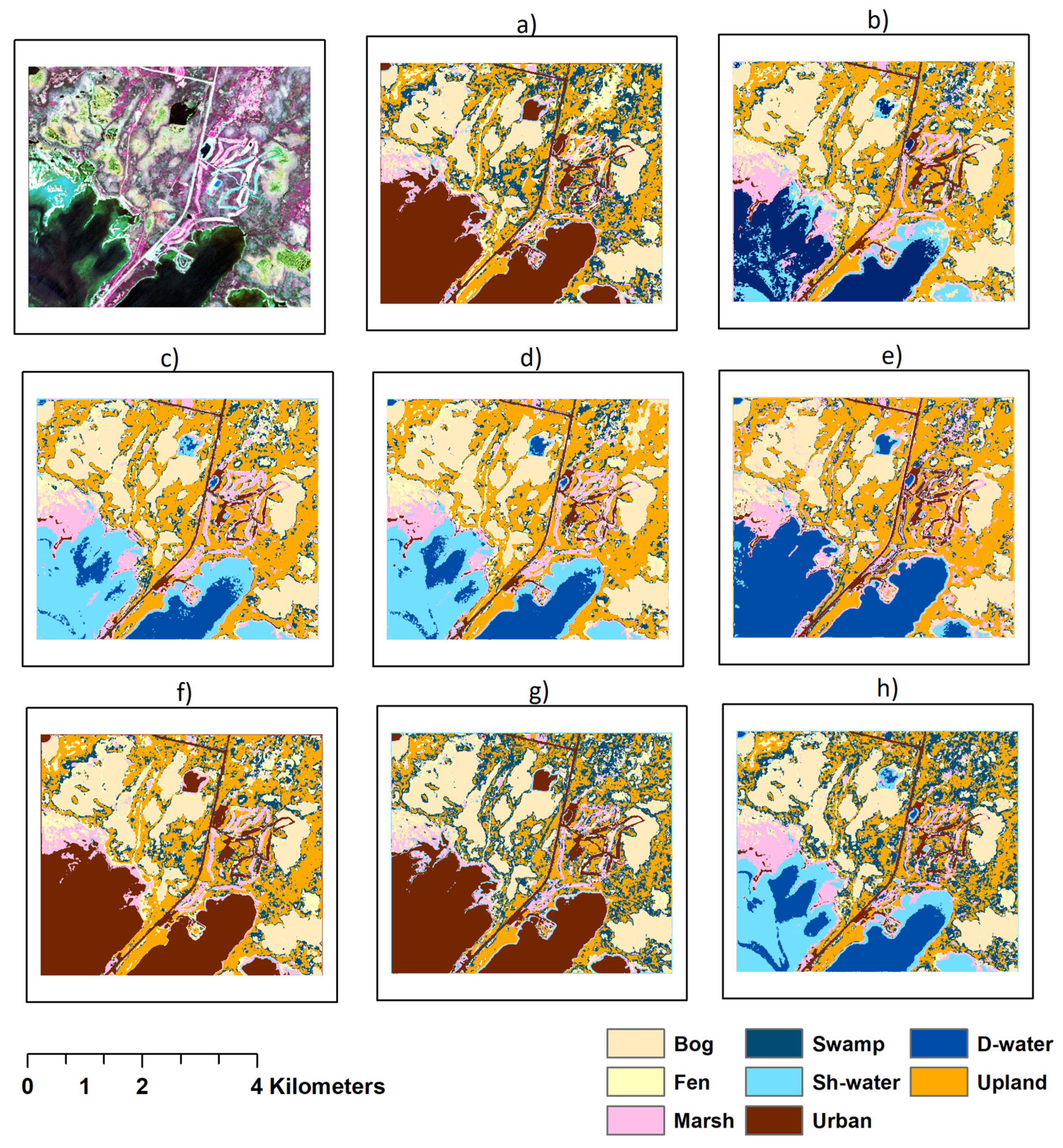
A part of the Gros Morne study area with about 4.2 km by 4.9 km was used for the classification mapping (Figure 15). In the Gros Morne region, the same issue exists for the incorrect classification of bog, fen, and marsh with solo CNN models. Most of the swamp areas were recognized as the upland class, and most of the CNNs had an issue with the correct classification of shallow and deep waters. It is worth mentioning that swamp and upland classes may have similar structure and vegetation types, specifically in the low water seasons. Consequently, their spectral reflectance can be similar, which leads to their misclassifications. Generally, wetlands are a complex environment where some of their classes have similar spectral signatures, specifically, bog, fen, and marsh wetland classes. All the solo CNNs presented a high level of accuracy for the classification of non-wetlands classes of urban, deep water, and uplands (Table 5 and Figure 15). In this study area similar to the Avalon, there were fewer training data for wetland classes of fen, marsh, swamp, and shallow water. Consequently, the performance of the solo CNNs was relatively poor compared to the Grand Falls. Moreover, as the number of training data for non-wetland classes of deep water and upland and wetland class of bog was higher in this region, the achieved overall accuracy was higher than the Avalon and Grand Falls. With an overall accuracy of 90.14%, the Inception-ResNet network was superior over the other solo CNNs (Figure 11 and Figure 14 and Table 5).
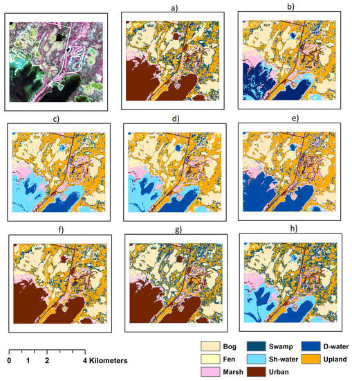
Figure 15.
Map of a part of the Gros Morne area showing the classification results of the CNN models using (a) DenseNet, (b) GoogLeNet, (c) Inception-ResNet, (d) MobileNet, (e) ResNet101, (f) ResNet18, (g) ShuffleNet, and (h) Xception.

Table 5.
The producer’s accuracy of the CNNs for the Gros Morne region (in percent).
There were more training data for bog, urban, deep water, and upland classes in the Avalon and Gros Morne. As a result, CNN models including MobileNet and Inception-ResNet with more parameters outperformed the CNN networks of ShuffleNet and GoogLeNet with fewer parameters.
4.4. Results of Ensemble Models
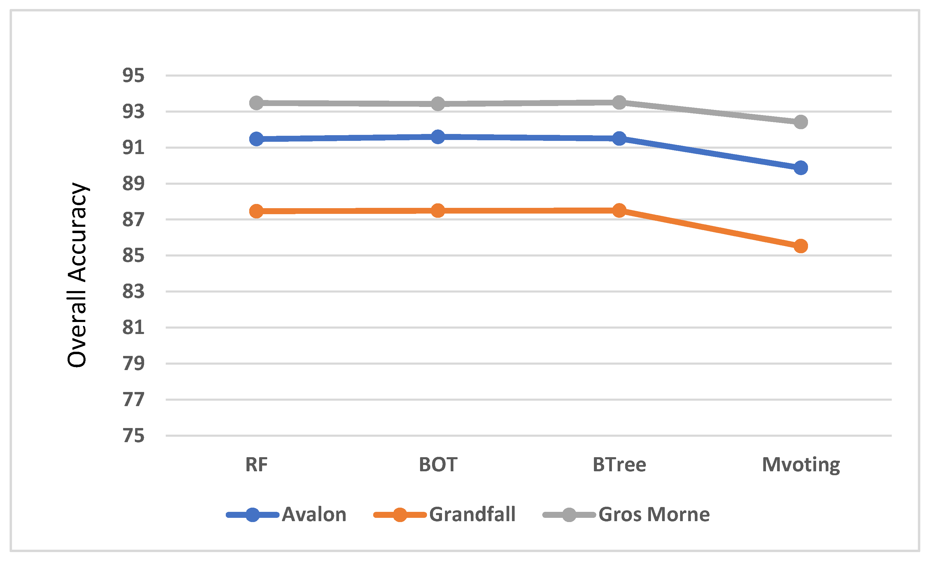
In this study, the main objective of integrating CNN models is to improve the wetland classification accuracy. As such, the probability layers extracted from the three solo CNN models with the highest accuracy for wetland classification in each study area were fused using four different approaches, which are RF, BTree, BOT, and majority voting. The overall accuracy from a comparison of predicted and reference classes is presented in Figure 16. Overall, RF, BOT, and BTree models showed higher accuracy in the Gros Morne region, followed by the Avalon and Grand Falls regions. In the Avalon area, the BOT classifier improved the overall accuracy of wetland classes by 6.43% through the ensemble of CNN models of DenseNet, ResNet18, and Xception networks (i.e., they had better results for wetland classification). Overall accuracy between the reference and predicted classes in the Avalon were generally lower compared to that of the Gros Morne study area. With the ensemble of Inception-ResNet, Xception, and MobileNet using the BTree algorithm, the overall accuracy was improved by 3.36% in the Gros Morne study area. The Grand Falls had the least overall accuracy compared to that of the Avalon and Gros Morne, where the BTree obtained higher accuracy than the majority voting, BOT, and RF classifiers, improving the overall accuracy by about 8.16% using the ensemble of GoogLeNet, Xception, and MobileNet.
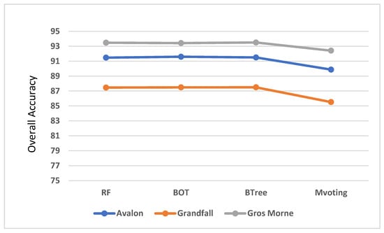
Figure 16.
The overall accuracy of the ensemble algorithms in the three study areas (in percent)..
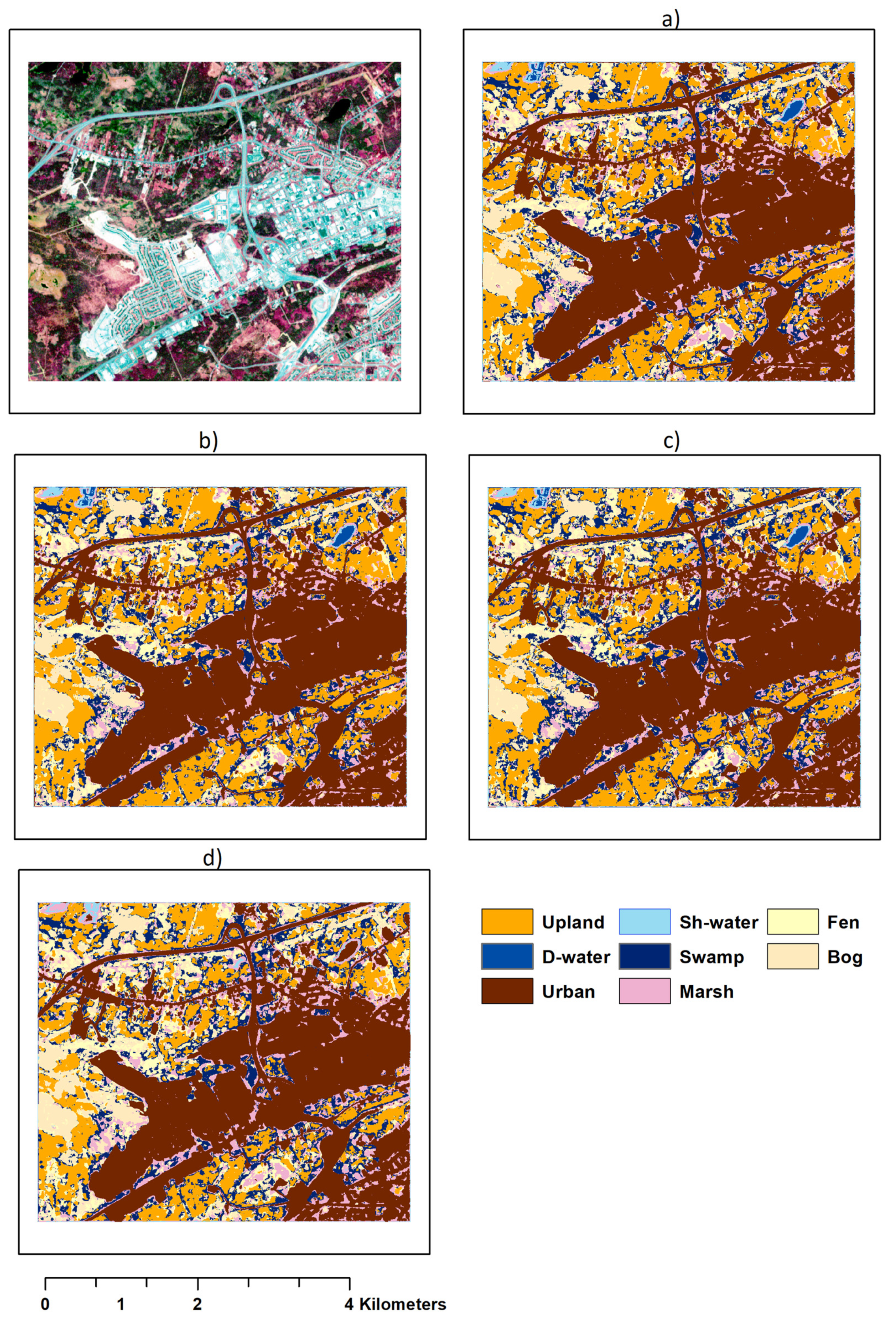
It can be seen that, in the Avalon region, the BTree classifier improved the results of the best solo CNN (i.e., MobileNet) for the classification of marsh, swamp, and fen classes by 36.68%, 25.76%, and 20.01%, respectively. However, the classification accuracies of shallow water and bog were decreased by 12.5% and 3.29%, respectively (Table 6 and Figure 17).

Table 6.
The producer’s accuracy of the ensemble models for the Avalon region (in percent).
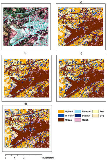
Figure 17.
Map of a part of the Avalon area based on the ensemble models using (a) BOT (b) BTree (c) RF (d) Majority voting.
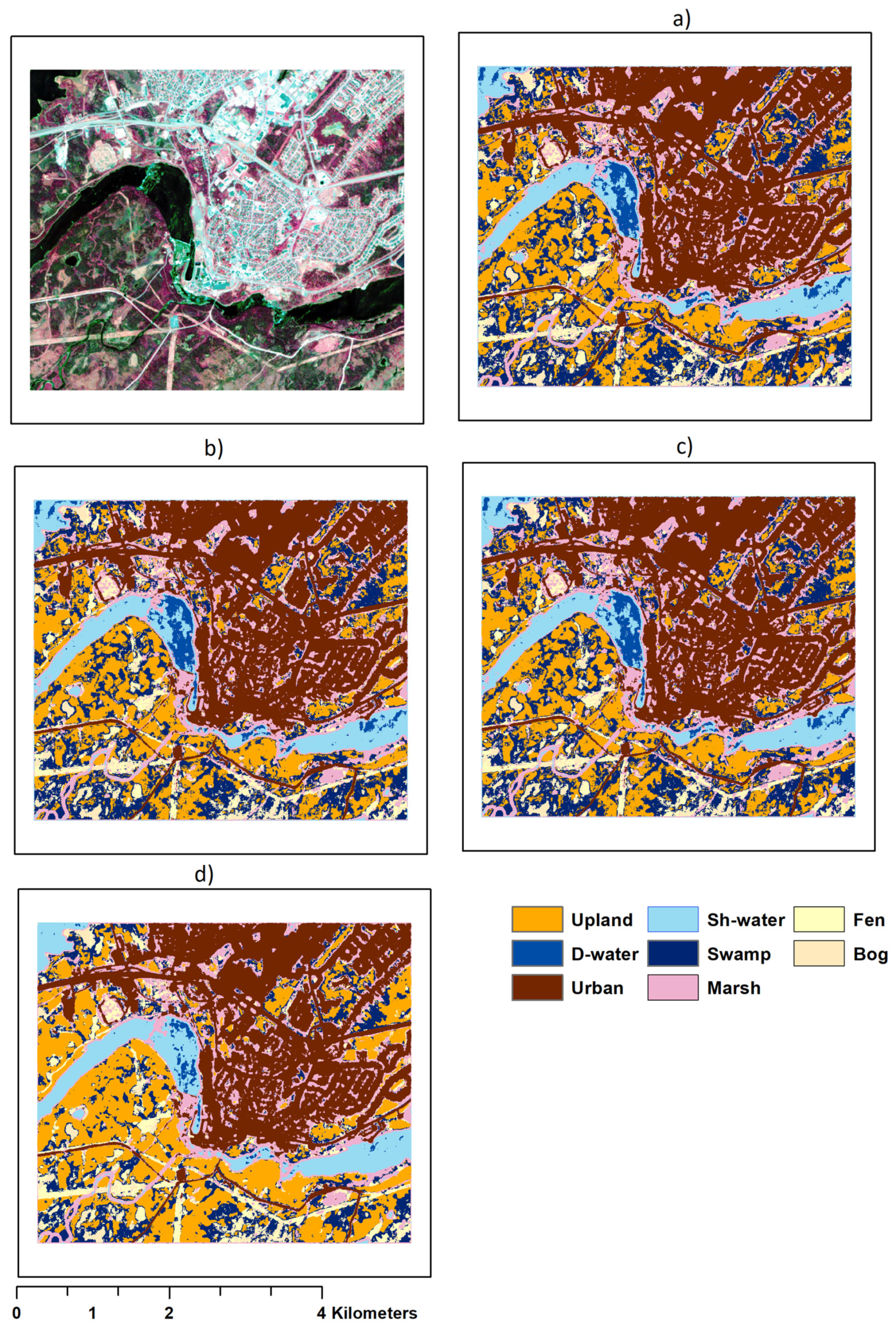
Results obtained by the BTree classifier indicated an improvement of the resulting shallow water, marsh, swamp, and bog classification of the best solo CNN (i.e., GoogLeNet) by 30.28%, 24.27%, 15.99%, and 5.72%, respectively. However, the classification accuracy of fen was decreased by 6.27%. The results of ensemble modeling indicated a significant improvement of wetland classification compared to that of the solo CNNs (Table 7 and Figure 18).

Table 7.
The producer’s accuracy of the ensemble models for the Grand Falls region (in percent).
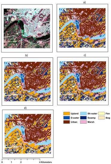
Figure 18.
Map of a part of the Grand Falls area based on the ensemble models using (a) BOT (b) BTree (c) RF (d) Majority voting.
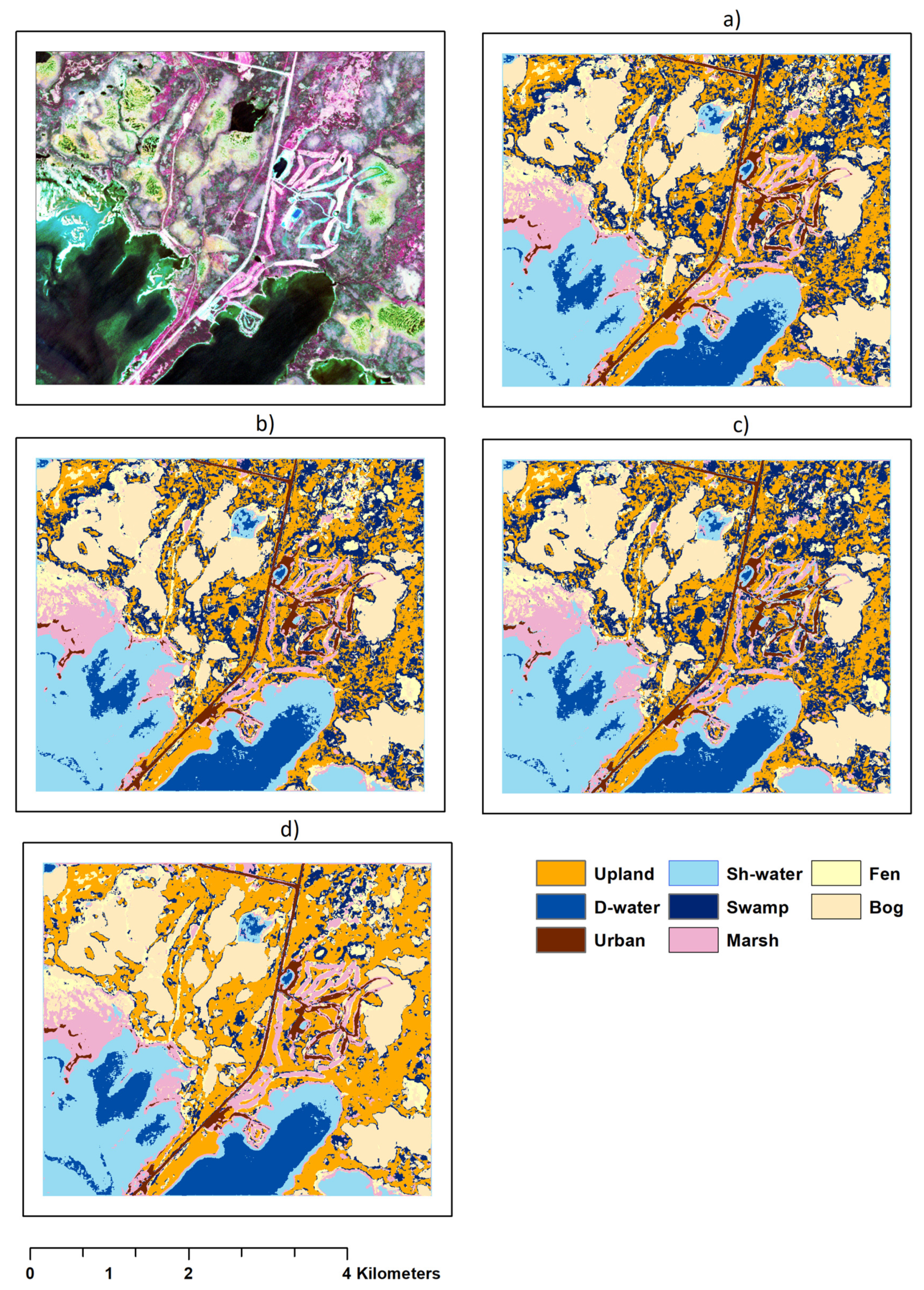
It is worth noting that, in the Gros Morne region, even though the overall accuracy did not increase substantially, the ensemble models achieved better classification accuracies for the wetland classes of swamp, fen, marsh, and shallow water. In more detail, the classification accuracy of these classes improved by 62.06%, 32.95%, 26.09%, and 9.79%, respectively, using the BTree classifier compared to that of the best solo CNN (i.e., Inception-ResNet) (Table 8 and Figure 19). Although, the classification accuracy of bog was decreased by 14.38%.

Table 8.
The producer’s accuracy of the ensemble models for the Gros Morne region (in percent).
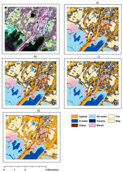
Figure 19.
Map of a part of the Gros Morne area based on the ensemble models using (a) BOT (b) BTree (c) RF (d) Majority voting.
To evaluate the efficiency and effectiveness of the solo CNNs and ensemble models for the classification of the wetland classes of bog, fen, marsh, swamp, and shallow water, their mean producer’s accuracy was assessed and summarized in Figure 20.
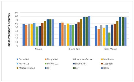
Figure 20.
The mean of producer’s accuracy for five wetland classes of bog, fen, marsh, swamp, and shallow water in the Avalon, Grand Falls, and Gros Morne.
The comparison revealed the superiority of the ensemble models compared to the solo CNN networks in terms of the mean producer’s accuracy. Results indicated a strong agreement between the predicted and reference wetland classes in the Gros Morne region using the ensemble models. In more detail, the ensemble model of the RF algorithm had the highest accuracy with a mean producer’s accuracy of 78%, where it improved the results of the best solo CNN model for the wetland classification (i.e., Xception with a mean producer’s accuracy of 58.96%) by more than 19%. In the Grand Falls, the ensemble model of the BTree improved the accuracy of the best solo CNN model (i.e., Xception with a mean producer’s accuracy of 63.51%) by 16.7%, with a mean producer’s accuracy of 80.21%. Finally, the Avalon area had the least agreement between the predicted and reference wetland classes using the ensemble models.
The BTree classifier improved the results of the best solo CNN model of ResNet18 (with a mean producer’s accuracy of 61.96%) by 9.63%, with a mean producer’s accuracy of 71.59%. Results obtained by the solo and ensemble CNNs indicated the advantage of shallower CNN models, including ResNet18 and Xception, over very deep learning models, such as DenseNet. Besides that, classification accuracies achieved by the solo CNN models were substantially improved in all three study areas for the wetland classification of bog, fen, marsh, swamp, and shallow water (Table 6, Table 7 and Table 8).
The number of parameters that are required to be fine-tuned for each solo CNNs is presented in Table 9. It is evident from Table 9 that Inception-ResNet, ResNet101, and MobileNet CNN networks with approximately 50.2, 42.5, and 40.5 million parameters, respectively, had the highest number of parameters that are required to be fine-tuned. On the other hand, the CNN networks of ShuffleNet, GoogLeNet, and ResNet18 with about 1, 6, and 11.2 million parameters, respectively, had the least number of parameters.

Table 9.
The number of parameters required to be fine-tuned in each solo CNN model utilized in this research.
The solo CNNs with a higher number of parameters (e.g., Inception-ResNet) require a higher number of training data to reach their full classification potential capability. This contrasts with the situation in remote sensing applications, specifically in wetland classification. As discussed in the previous sections, creating a high number of training data is labor-intensive and quite costly in remote sensing. Overall, this research demonstrated that with a limited number of training data, CNN networks with fewer parameters had better classification performance (e.g., ShuffleNet).
Moreover, the results demonstrated that the supervised classifiers, including BTree, BOT, and RF, were superior in terms of the overall accuracy and mean producer’s accuracy over the unsupervised classifier of majority voting in the Avalon, Grand Falls, and Gros Morne. Their different strategy of data fusion can explain their better classification results. In majority voting classifier, results of the best CNNs are simply fused by their majority values. In contrast, in the supervised tree-based classifiers such as BTree algorithm, results are trained once more to minimize the classification error, resulting in much better classification accuracy.
5. Conclusions
Due to the valuable benefits obtained by humans and Nature provided by wetland functions, new techniques and technologies for wetland mapping/monitoring are of great importance. Wetlands are considered among the most complex ecosystems to classify due to their dynamic and complex structure with no clear-cut boundaries with similar vegetation structures. In this regard, for high-resolution complex wetland classification, the results of various solo CNN models, including DenseNet, GoogLeNet, ShuffleNet, MobileNet, Xception, Inception-ResNet, ResNet18, and ResNet101, were compared and evaluated against several proposed ensemble-based approaches. Regarding the solo CNNs, due to the different number of existing training data in each study area, obtained results were relatively inconsistent. For example, in the Grand Falls, the number of training data for wetland classes was higher than the other two study regions, resulting in a better producer’s accuracy in this region. The overall accuracy of the solo CNNs was low in the Grand Falls; the number of training data for non-wetland classes was less than the Avalon and Gros Morne (overall accuracy ranged from 73.87% to 79.34%). In addition, in both the Avalon and Gros Morne, producer’s accuracy for the classification of wetlands was low due to the limited number of wetlands training in these regions.
In contrast, in the Avalon and Gros Morne, their overall accuracy was better, resulting from a higher number of training data of non-wetlands. It was concluded that the classification performances of the solo CNNs highly depend on the existing training data, specifically, deeper CNNs such as Inception-ResNet and DenseNet with a higher number of parameters (Table 3, Table 4 and Table 5). Overall, CNNs with fewer parameters to be fine-tuned (i.e., ShuffleNet) were more successful in recognizing wetlands in terms of classification accuracy (Figure 11). On the other hand, the proposed ensemble of solo CNNs using the results of the best three CNNs in each study area significantly improved the classification accuracy of wetlands (Table 6, Table 7 and Table 8). The ensemble models were superior over the solo CNNs as they include one more classification step minimizing the classification error of the solo CNNs, specifically for wetland classification. The classification results of the solo CNNs improved by the supervised classifiers of BTree, BOT, and RF and the unsupervised algorithms of majority voting in terms of the mean producer’s accuracy by 9.63%, 16.7%, and 19.04% in the Avalon, Grand Falls, and Gros Morne, respectively.
Author Contributions
Conceptualization, A.J. and M.M.; methodology, A.J. and M.M.; formal analysis, A.J. and M.M.; writing—original draft preparation, A.J. and M.M.; writing—review and editing, A.J., M.M., B.B., J.G., F.M., and B.S.; supervision, M.M., B.B., J.G., F.M., and B.S.; funding acquisition, M.M. All authors have read and agreed to the published version of the manuscript.
Funding
This research received no external funding.
Institutional Review Board Statement
Not applicable.
Informed Consent Statement
Not applicable.
Data Availability Statement
Not applicable.
Conflicts of Interest
The authors declare no conflict of interest.
References
- Slagter, B.; Tsendbazar, N.-E.; Vollrath, A.; Reiche, J. Mapping wetland characteristics using temporally dense Sentinel-1 and Sentinel-2 data: A case study in the St. Lucia wetlands, South Africa. Int. J. Appl. Earth Obs. Geoinf. 2020, 86, 102009. [Google Scholar] [CrossRef]
- Mahdianpari, M.; Granger, J.E.; Mohammadimanesh, F.; Salehi, B.; Brisco, B.; Homayouni, S.; Gill, E.; Huberty, B.; Lang, M. Meta-Analysis of Wetland Classification Using Remote Sensing: A Systematic Review of a 40-Year Trend in North America. Remote Sens. 2020, 12, 1882. [Google Scholar] [CrossRef]
- Tiner, R.W. Wetlands: An overview. In Remote Sensing of Wetlands: Applications and Advances; Tiner, R.W., Lang, M.W., Klemas, V.V., Eds.; CRC Press: Boca Raton, FL, USA, 2015; pp. 20–35. [Google Scholar]
- Board, M.A. Millennium Ecosystem Assessment; New Island: Washington, DC, USA, 2005. [Google Scholar]
- Davidson, N.C. The Ramsar Convention on Wetlands. In The Wetland Book I: Structure and Function, Management and Methods; Springer Publishers: Dordrecht, The Netherlands, 2016. [Google Scholar]
- Bansal, J.C. Particle swarm optimization. In Evolutionary and Swarm Intelligence Algorithms; Springer: Cham, Switzerland, 2019; Volume 779, pp. 11–23. [Google Scholar]
- Mahdianpari, M.; Salehi, B.; Mohammadimanesh, F.; Homayouni, S.; Gill, E. The First Wetland Inventory Map of Newfoundland at a Spatial Resolution of 10 m Using Sentinel-1 and Sentinel-2 Data on the Google Earth Engine Cloud Computing Platform. Remote Sens. 2018, 11, 43. [Google Scholar] [CrossRef]
- Bansal, S.; Katyal, D.; Garg, J. A novel strategy for wetland area extraction using multispectral MODIS data. Remote Sens. Environ. 2017, 200, 183–205. [Google Scholar] [CrossRef]
- Chatziantoniou, A.; Psomiadis, E.; Petropoulos, G.P. Co-Orbital Sentinel 1 and 2 for LULC Mapping with Emphasis on Wetlands in a Mediterranean Setting Based on Machine Learning. Remote Sens. 2017, 9, 1259. [Google Scholar] [CrossRef]
- Stratoulias, D.; Balzter, H.; Sykioti, O.; Zlinszky, A.; Tóth, V.R. Evaluating Sentinel-2 for Lakeshore Habitat Mapping Based on Airborne Hyperspectral Data. Sensors 2015, 15, 22956–22969. [Google Scholar] [CrossRef] [PubMed]
- Mahdianpari, M.; Salehi, B.; Rezaee, M.; Mohammadimanesh, F.; Zhang, Y. Very Deep Convolutional Neural Networks for Complex Land Cover Mapping Using Multispectral Remote Sensing Imagery. Remote Sens. 2018, 10, 1119. [Google Scholar] [CrossRef]
- Rezaee, M.; Mahdianpari, M.; Zhang, Y.; Salehi, B. Deep Convolutional Neural Network for Complex Wetland Classification Using Optical Remote Sensing Imagery. IEEE J. Sel. Top. Appl. Earth Obs. Remote Sens. 2018, 11, 3030–3039. [Google Scholar] [CrossRef]
- Wen, L.; Hughes, M. Coastal Wetland Mapping Using Ensemble Learning Algorithms: A Comparative Study of Bagging, Boosting and Stacking Techniques. Remote Sens. 2020, 12, 1683. [Google Scholar] [CrossRef]
- Zhang, A.; Sun, G.; Ma, P.; Jia, X.; Ren, J.; Huang, H.; Zhang, X. Coastal Wetland Mapping with Sentinel-2 MSI Imagery Based on Gravitational Optimized Multilayer Perceptron and Morphological Attribute Profiles. Remote Sens. 2019, 11, 952. [Google Scholar] [CrossRef]
- Jamali, A. Land use land cover modeling using optimized machine learning classifiers: A case study of Shiraz, Iran. Model. Earth Syst. Environ. 2020, 1–12. [Google Scholar] [CrossRef]
- Jamali, A. Improving land use land cover mapping of a neural network with three optimizers of multi-verse optimizer, genetic algorithm, and derivative-free function. Egypt. J. Remote Sens. Space Sci. 2020. [Google Scholar] [CrossRef]
- Jamali, A. Land use land cover mapping using advanced machine learning classifiers: A case study of Shiraz city, Iran. Earth Sci. Informatics 2020, 13, 1015–1030. [Google Scholar] [CrossRef]
- Moayedi, H.; Jamali, A.; Gibril, M.B.A.; Foong, L.K.; Bahiraei, M. Evaluation of tree-base data mining algorithms in land used/land cover mapping in a semi-arid environment through Landsat 8 OLI image; Shiraz, Iran. Geomat. Nat. Hazards Risk 2020, 11, 724–741. [Google Scholar] [CrossRef]
- Ji, S.; Zhang, C.; Xu, A.; Shi, Y.; Duan, Y. 3D Convolutional Neural Networks for Crop Classification with Multi-Temporal Remote Sensing Images. Remote Sens. 2018, 10, 75. [Google Scholar] [CrossRef]
- Krizhevsky, A.; Sutskever, I.; Hinton, G.E. Imagenet classification with deep convolutional neural networks. Adv. Neural Inf. Process. Syst. 2012, 25, 1097–1105. [Google Scholar] [CrossRef]
- Shao, Z.; Cai, J. Remote Sensing Image Fusion With Deep Convolutional Neural Network. IEEE J. Sel. Top. Appl. Earth Obs. Remote Sens. 2018, 11, 1656–1669. [Google Scholar] [CrossRef]
- Zhang, C.; Pan, X.; Li, H.; Gardiner, A.; Sargent, I.; Hare, J.; Atkinson, P.M. A hybrid MLP-CNN classifier for very fine resolution remotely sensed image classification. ISPRS J. Photogramm. Remote Sens. 2018, 140, 133–144. [Google Scholar] [CrossRef]
- Sedona, R.; Cavallaro, G.; Jitsev, J.; Strube, A.; Riedel, M.; Benediktsson, J.A. Remote Sensing Big Data Classification with High Performance Distributed Deep Learning. Remote Sens. 2019, 11, 3056. [Google Scholar] [CrossRef]
- DeLancey, E.R.; Simms, J.F.; Mahdianpari, M.; Brisco, B.; Mahoney, C.; Kariyeva, J. Comparing Deep Learning and Shallow Learning for Large-Scale Wetland Classification in Alberta, Canada. Remote Sens. 2019, 12, 2. [Google Scholar] [CrossRef]
- Redmon, J.; Divvala, S.; Girshick, R.; Farhadi, A. You only look once: Unified, real-time object detection. In Proceedings of the IEEE Conference On Computer Vision And Pattern Recognition, Las Vegas, NV, USA, 27–30 June 2016; pp. 779–788. [Google Scholar]
- Redmon, J.; Farhadi, A. YOLO9000: Better, faster, stronger. In Proceedings of the IEEE Conference on Computer Vision and Pattern Recognition, Honolulu, HI, USA, 21–26 July 2017; pp. 7263–7271. [Google Scholar]
- Taghizadeh-Mehrjardi, R.; Mahdianpari, M.; Mohammadimanesh, F.; Behrens, T.; Toomanian, N.; Scholten, T.; Schmidt, K. Multi-task convolutional neural networks outperformed random forest for mapping soil particle size fractions in central Iran. Geoderma 2020, 376, 114552. [Google Scholar] [CrossRef]
- Pan, X.; Zhao, J. A central-point-enhanced convolutional neural network for high-resolution remote-sensing image classification. Int. J. Remote Sens. 2017, 38, 6554–6581. [Google Scholar] [CrossRef]
- Jamali, A.; Mahdianpari, M.; Brisco, B.; Granger, J.; Mohammadimanesh, F.; Salehi, B. Wetland Mapping Using Multi-Spectral Satellite Imagery and Deep Convolutional Neural Networks: A Case Study in Newfoundland and Labrador, Canada. Can. J. Remote Sens. 2021, 1–18. [Google Scholar] [CrossRef]
- Jeppesen, J.H.; Jacobsen, R.H.; Inceoglu, F.; Toftegaard, T.S. A cloud detection algorithm for satellite imagery based on deep learning. Remote Sens. Environ. 2019, 229, 247–259. [Google Scholar] [CrossRef]
- Mohammadimanesh, F.; Salehi, B.; Mahdianpari, M.; Gill, E.; Molinier, M. A new fully convolutional neural network for semantic segmentation of polarimetric SAR imagery in complex land cover ecosystem. ISPRS J. Photogramm. Remote Sens. 2019, 151, 223–236. [Google Scholar] [CrossRef]
- Han, M.; Feng, Y.; Zhao, X.; Sun, C.; Hong, F.; Liu, C. A Convolutional Neural Network Using Surface Data to Predict Subsurface Temperatures in the Pacific Ocean. IEEE Access 2019, 7, 172816–172829. [Google Scholar] [CrossRef]
- Ji, M.; Liu, L.; Du, R.; Buchroithner, M.F. A Comparative Study of Texture and Convolutional Neural Network Features for Detecting Collapsed Buildings After Earthquakes Using Pre- and Post-Event Satellite Imagery. Remote Sens. 2019, 11, 1202. [Google Scholar] [CrossRef]
- Newfoundland and Labrador Fisheries and Land Resources, “High Boreal Forest Ecoregion”. Government of Newfoundland and Labrador. 2008. Available online: https://www.gov.nl.ca/flr/files/publications-parks-ecoregions-lab-6-high-boreal.pdf (accessed on 29 July 2020).
- Amani, M.; Salehi, B.; Mahdavi, S.; Brisco, B. Spectral analysis of wetlands using multi-source optical satellite imagery. ISPRS J. Photogramm. Remote Sens. 2018, 144, 119–136. [Google Scholar] [CrossRef]
- Szegedy, C.; Liu, W.; Jia, Y.; Sermanet, P.; Reed, S.; Anguelov, D.; Erhan, D.; Vanhoucke, V.; Rabinovich, A. Going deeper with convolutions. In Proceedings of the IEEE conference on computer vision and pattern recognition, Boston, MA, USA, 7–12 June 2015; Volume 1, pp. 1–9. [Google Scholar]
- Hoeser, T.; Kuenzer, C. Object Detection and Image Segmentation with Deep Learning on Earth Observation Data: A Review-Part I: Evolution and Recent Trends. Remote Sens. 2020, 12, 1667. [Google Scholar] [CrossRef]
- Qin, Z.; Zhang, Z.; Chen, X.; Wang, C.; Peng, Y. Fd-mobilenet: Improved mobilenet with a fast downsampling strategy. In Proceedings of the 2018 25th IEEE International Conference on Image Processing (ICIP), Athens, Greece, 7–10 October 2018; pp. 1363–1367. [Google Scholar] [CrossRef]
- Chollet, F. Xception: Deep Learning with Depthwise Separable Convolutions. In Proceedings of the IEEE Conference on Computer Vision and Pattern Recognition (CVPR), Honolulu, HI, USA, 21–26 July 2017; pp. 1251–1258. [Google Scholar]
- Zhang, X.; Zhou, X.; Lin, M.; Sun, J. ShuffleNet: An Extremely Efficient Convolutional Neural Network for Mobile Devices. In Proceedings of the 2018 IEEE/CVF Conference on Computer Vision and Pattern Recognition, Salt Lake City, MA, USA, 18–23 June 2018; pp. 6848–6856. [Google Scholar]
- Xie, S.; Girshick, R.; Dollar, P.; Tu, Z.; He, K. Aggregated ’residual transformations for deep neural networks. In Proceedings of the IEEE Conference on Computer Vision and Pattern Recognition, Las Vegas, NV, USA, 27–30 June 2016; pp. 1492–1500. [Google Scholar]
- He, K.; Zhang, X.; Ren, S.; Sun, J. Deep residual learning for image recognition. In Proceedings of the IEEE Conference on Computer Vision and Pattern Recognition, Las Vegas, NV, USA, 27–30 June 2016; pp. 770–778. [Google Scholar]
- He, K.; Zhang, X.; Ren, S.; Sun, J. Identity mappings in deep residual networks. In ECCV 2016: Computer Vision—ECCV 2016; Springer: Cham, Switzerland, 2016; Volume 9908, pp. 630–645. [Google Scholar]
- Szegedy, C.; Ioffe, S.; Vanhoucke, V.; Alemi, A.A. Inception-v4, Inception-ResNet and the Impact of Residual Connections on Learning. In Proceedings of the Thirty-First AAAI Conference on Artificial Intelligence, San Francisco, CA, USA, 4–9 February 2017; Volume 31, pp. 4278–4284. [Google Scholar]
- Huang, G.; Liu, Z.; van der Maaten, L.; Weinberger, K.Q. Densely connected convolutional networks. In Proceedings of the IEEE Conference on Computer Vision and Pattern Recognition, Honolulu, HI, USA, 21–26 July 2017; pp. 4700–4708. [Google Scholar]
Publisher’s Note: MDPI stays neutral with regard to jurisdictional claims in published maps and institutional affiliations. |
© 2021 by the authors. Licensee MDPI, Basel, Switzerland. This article is an open access article distributed under the terms and conditions of the Creative Commons Attribution (CC BY) license (https://creativecommons.org/licenses/by/4.0/).

