Abstract
A long-term dataset of 38 years (1982–2019) from the Advanced Very High Resolution Radiometer (AVHRR) satellite observations is applied to investigate the spatio-temporal seasonal trends in cloud fraction, surface downwelling longwave flux, and surface upwelling longwave flux over the Arctic seas (60~90° N) by the non-parametric methods. The results presented here provide a further contribution to understand the cloud cover and longwave surface radiation trends over the Arctic seas, and their correlations to the shrinking sea ice. Our results suggest that the cloud fraction shows a positive trend for all seasons since 2008. Both surface downwelling and upwelling longwave fluxes present significant positive trends since 1982 with higher magnitudes in autumn and winter. The spatial distribution of the trends is nearly consistent between the cloud fraction and the surface longwave radiation, except for spring over the Chukchi and Beaufort Seas. We further obtained a significant negative correlation between cloud fraction (surface downwelling/upwelling longwave fluxes) and sea-ice concentration during autumn, which is largest in magnitude for regions with substantial sea ice retreat. We found that the negative correlation between cloud fraction and sea-ice concentration is not as strong as that for the surface downwelling longwave flux. It indicates the increase in cloudiness may result in positive anomalies in surface downwelling longwave flux which is highly correlated with the sea-ice retreat in autumn.
1. Introduction
Sea ice has been accepted to be the most significant component of the Arctic climate system. As an efficient barrier, the Arctic sea ice could limit absorbing solar energy and meanwhile reduce the flux exchanges (e.g., water vapor, momentum, and heat) between the atmosphere and the underlying ocean [1,2]. According to the Sea Ice Index derived from the National Snow and Ice Data Center (NSIDC), a persistent negative trend in Arctic sea ice is exhibited ever since November 1978, the initial time of satellite record. In recent decades, the rapid decline of sea ice [3,4,5,6,7] has come into notice, which indicates the Arctic climate has undergone significant changes.
Arctic climate is influenced by different physical parameters through negative or positive feedback [8,9,10,11]. Among these parameters, clouds and radiation, contributing to the Arctic sea-ice stability by the cloud-radiative process, have become the focus of studies [12,13,14,15]. It is well-known that clouds have an important influence on the net surface radiation budget. The changes in clouds could result in profound effects on the radiative balance [16,17]. The influence of clouds on the surface is determined by multiple cloud physical parameters [12]. The cloud amount/fraction is one of the most commonly used parameters in analyzing the cloud-radiation and sea ice interactions [18].
For further interpreting the complex feedbacks of clouds in the Arctic climate system, the trends and variations of the Arctic cloud cover with associated radiation are analyzed through in situ, satellite and reanalysis datasets, e.g., [19,20,21]. In general, the cloud fraction in Arctic shows a distinct annual cycle, e.g., [9,22,23]. Its maximum always appears from early summer to late autumn, and its minimum appears in late spring [20]. However, regarding the long-term trend of the Arctic cloud cover, different datasets or datasets with different time scales lead to different conclusions. Schweiger [24] used three independent long-term datasets (TIROS Operation Vertical Sounder (TOVS) Polar Pathfinder Retrieval (1980–2001), Advanced Very High Resolution Radiometer (AVHRR) Polar Pathfinder (APP) dataset (1982–1999), and another dataset (1981–2000) from AVHRR using a different algorithm) to compare cloud cover in winter and spring for 1982–1999. In their study, the authors reported a significant negative trend in winter cloudiness for the Arctic sea regions and a noticeable positive trend in spring cloudiness, especially over the Central Arctic [24]. Using APP dataset (1982–1999), Wang and Key [25] reported that Arctic cloud cover in spring and summer increased at about 0.32%/yr and 0.16%/yr, respectively, while in winter, it decreased at a rate of −0.60%/yr. On the contrary, from the AVHRR data during 1981–2000, Comiso [26] found that the cloudiness showed negative trends in all seasons, except for summer Greenland with a positive trend at 0.30%/yr. A recent publication [27], through analyzing a dataset of 16 years (2000–2015) derived from the Clouds and Earth’s Radiant Energy System (CERES) [28], found that for the September sea-ice retreat regions from 1 March to 14 May, the cloud amount showed a positive trend, while from 15 May to 28 June, it showed a negative trend. There have been many more studies about the long-term trend of Arctic cloud cover and the interactions between clouds and sea ice, which still need further investigation.
Previous studies have attempted to analyze the cloud-radiation interaction and its correlations with the Arctic sea-ice melting [12,18,29,30,31,32,33]. In general, Arctic clouds are supposed to maintain a warming effect for all seasons except a brief period of cooling in summer [12,18,30,32]. Some studies showed that the springtime clouds and surface longwave radiation may contribute to the sea-ice decline. For example, the study by Kapsch et al. proved that the springtime longwave radiation to the surface could be a key parameter that promoted the melting of the Arctic sea ice [34]. A recent study [27] found that during springtime the increasing downward longwave flux tended to enhance sea-ice melting as well. The results from climate model also revealed that in spring and early summer positive anomalies of the longwave radiation to the surface have a considerable impact on the extent of sea ice in September [10]. Some studies focused on the relationships between autumnal clouds and sea-ice variations. Schweiger et al. pointed out that the cloud cover near the sea-ice edge was closely related to the sea-ice changes through the study of the relationships between autumnal Arctic clouds and sea ice [35]. Wu and Lee found that during autumn the enhanced warming air temperature near surface could be caused by the increasing clouds in October, which may result in the Arctic sea-ice decline [36]. A recent study [37] proposed the importance of the interactions in winter. They found that in winter the large sea-ice loss may strengthen the upward transport of water vapor and thus promote the cloud formation. This could further result in considerable longwave radiative forcing and enhance the relationship between clouds, moisture, and temperature in the lower troposphere [37].
The above research results show that there are complex inter-correlations between Arctic clouds, radiation, and sea ice. Long-term datasets would provide useful help in understanding the relationships between them. As it is extremely challenging to obtain long-term continuous ground-based observations due to the harsh weather in the Arctic, the observations from satellite are critically required to investigate the interactions between Arctic clouds, radiation, and sea ice. This study is based on the satellite dataset of AVHRR Polar Pathfinder-Extended (APP-x) project.
In purview of the above, previous studies are predominately focused on the trends or variability of individual seasons and lack of comparisons between seasons. This study aims at further investigating the seasonal trends and variations in clouds and surface longwave radiation over the Arctic seas by the APP-x dataset from 1982 to 2019. In particular, this study will present a temporal and spatial analysis of cloud fraction (CF), surface downwelling longwave flux (DLF), and surface upwelling longwave flux (ULF) for all seasons and examine their possible connections with the autumn sea ice. As a result, the manuscript is arranged as follows: Section 2 explains the data and research methods. Section 3 shows the key study results and related discussions. Finally, the discussion and key research conclusions together with some suggestions for continuing further the present research are summarized in Section 4 and Section 5, respectively.
2. Materials and Methods
2.1. Data
APP-x, a thematic climate data record (CDR), is derived from APP dataset (navigated and calibrated AVHRR data) [38]. It provides continuous daily data, including surface and cloud characteristic parameters as well as radiant flux in polar regions ever since 1982 [25,38,39,40]. The daily dataset consists of two separate processing time at 04:00 and 14:00 local solar time (LST) [38]. All data are projected on the Equal-Area Scalable Earth (EASE) gridding map with a resolution of 25 km.
The APP-x version 2 dataset is used in this study. The detailed algorithm descriptions and corresponding improvements are given in the references [41,42]. The dataset contains 19 geophysical variables. The DLF, ULF, and cloud mask, which are marked as CDR quality, are applied for the following analysis. Products were validated by the data from the Surface HEat Budget of the Arctic (SHEBA) experiment. It was reported that the biases of CF, DLF, and ULF were 0.14, 2.1 Wm−2, and 1.9 Wm−2, with the root-mean-square error (RMSE) of 0.26, 22.4 Wm−2, and 9.4 Wm−2 [25,38,39]. The time series of APP-x dataset are completed except for the period from September to December of 1994 due to partial data missing. We computed monthly data based on the valid daily data. The monthly cloud fraction is derived from the daily cloud mask.
The Passive Microwave Sea Ice Concentration (version 3) product, provided by NSIDC/NOAA, is applied here for the sea ice concentration (SIC) analysis [43,44,45,46]. This dataset provides a CDR of SIC based on passive microwave observations. The outputs from two well-established algorithms, including the NASA Team (NT) algorithm [47] and NASA Bootstrap (BT) algorithm [48], are combined by defined rules to generate the SIC product. It was reported that the bias is +1.0~+3.5% during winter [49] and +5~+10% during summer in Arctic [50]. It provides daily and monthly SIC since 9 July 1987 for both the Arctic and Antarctic. The SIC product is processed on a 25 × 25 km EASE grid. For long-term analysis, the monthly SIC data from July 1987 to December 2019 are selected here.
2.2. Methods
In order to analyze the long-term trends in Arctic clouds and radiation, the Mann–Kendall and Sen’s slope statistical tests are applied in this study. The Mann–Kendall test is an important statistical trend analysis technique. It belongs to the non-parametric methods, which only require that the data to be analyzed be independent [51,52]. It is commonly applied for the time series datasets. The statistic S applied in the Mann–Kendall test is estimated according to
n represents the total number of the data in time series, j and k represent the index of time series , and represent the values of the data of time indices j and k. represent the sign as
when , the variance is calculated as
The data with the same value are classified into clusters. m is the total number of clusters. represents the total number of data included into the jth cluster. The statistic Zs is approximately normal distributed and calculated as
Zs with a negative value represents a decreasing trend, while Zs with a positive value represents an upward trend. The trend analysis is required at the specific α significance level. The null hypothesis is rejected when . Thus, the analyzed trend indicates to be significant. could be acquired by the standardized normal distribution look-up table. Here, the significance levels of 99% (α = 0.01) and 95% (α = 0.05) are applied while and .
The Sen’s slope statistical test [53] is widely applied to analyze hydro-meteorological time series. This method proposed a slope estimator to provide an estimation for the trend slope of the time series dataset.
A series of linear slopes could be estimated as
and represent the values of the data with indices j and k ; N represents the pairs of data. could be calculated as requiring only one datum at each time point, where represent the number of time points. The estimator is determined as the median value in slope series. The sign of β represents increasing (positive) or decreasing (negative) trend, while the magnitude of the trend is represented by the value of .
Using the non-parametric method based on the normal distribution, a two-sided test at the 100 (1–α)% confidence interval is applied here [54,55]. The confidence interval could be calculated as
is estimated by the standardized normal distribution look-up table. has been defined in Equation (3).
Here, the significance levels of 99% (α = 0.01) and 95% (α = 0.05) are applied. and , defined as the upper and lower limits of the confidence interval, represent the (K2 + 1)th and the K1th largest of the N ordered slope estimates. K1 and K2 are calculated as
If and have similar sign, then the estimator is statistically different than zero.
3. Results
The research interests are focused primarily on the Arctic sea regions from 60° N to 90° N (Figure 1). Figure 1 displays the specific sub-regions as well for detailed analysis. The seasons involved here are defined as follows: spring as MAM (March to May), summer as JJA (June to August), autumn as SON (September to November), and winter as DJF (December of this year and January and February of the following year).
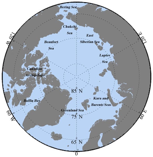
Figure 1.
Study regions (light blue) from 60° N to 90° N. The land areas are masked in gray.
3.1. Temporal Trends
The seasonal cycles of the CF, DLF, and ULF over the seas in Arctic (60°~90° N) are shown in Figure 2 for 04:00 LST in black and 14:00 LST in red. Figure 2a shows the highest cloud cover occurs in summer, with the mean values being 71.6% at 04:00 LST and 78.1% at 14:00 LST, respectively. There are fewer clouds in spring, with the minimum values being 65.8% at 04:00 LST and 60.8% at 14:00 LST in April. Figure 2a also shows that except for March and April, the CF at 14:00 LST is always larger than that at 04:00 LST, indicating that the cloud fraction in the afternoon over the Arctic seas is higher than that in the early morning. In the first two months of spring, the CF at 14:00 LST is lower than that at 04:00 LST. In summer, the CF at 04:00 LST reaches its maximum value of the year in June, and then decreases month by month. At 14:00 LST, the CF reaches the maximum value in August. The maximum CF difference between 04:00 LST and 14:00 LST also appeared in August. The annual variation of CF is consistent with the conclusions reported by Chernokulsky and Mokhov [20]. Based on 16 separate cloud climatology datasets from satellite, re-analyses, and surface observations, they found that there is a significant annual cycle for the total cloud fraction in the Arctic. The time of CF maximum occurred during the early summer to late autumn, and the minimum appeared during late spring [20].
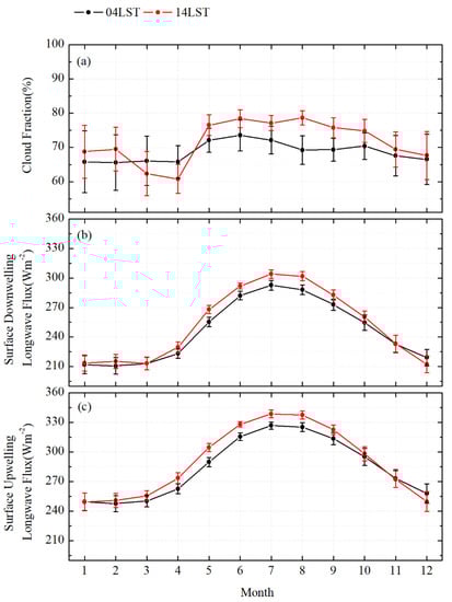
Figure 2.
Seasonal variations of (a) CF, (b) DLF, and (c) ULF averaged over the seas in Arctic from 60° N to 90° N from 1982 to 2019 at 04:00 LST (black) and 14:00 LST (red). Bars represent ± standard deviation of the mean.
As shown in Figure 2b,c, the seasonal cycles of DLF and ULF are more prominent and follow unimodal distribution. The higher values appear in summer, while lower values appear in winter and spring. Starting from May, DLF shows a significant increase and reach higher values in summer. After that, DLF decreases month by month. There is a significant decline in November and a relatively stable low DLF value maintaining in winter and early spring. The ULF has a similar pattern as DLF. The maximum values attain in July with 292.6 Wm−2 at 04:00 LST (304.0 Wm−2 at 14:00 LST) of DLF, and 326.6 Wm−2 at 04:00 LST (338.5Wm−2 at 14:00 LST) of ULF. Based on the APP-x product during 1982–1999, Wang and Key also found that the largest DLF and ULF occurred in July [39]. Comparing Figure 2b,c, it can also be observed that the ULF is significantly higher than the DLF at both 04:00 LST and 14:00 LST. Moreover, except for December, the DLF or ULF of 14:00 LST is relatively higher than (and close to) that of 04:00 LST.
Figure 3 shows the time series of seasonal CF at 04:00 LST and 14:00 LST. There are two obvious features about the seasonal CF variations. One is that the variations of long-term CF between seasons are different. Generally, the CF in MAM, JJA, and SON keeps a relatively stable level, with low standard deviation (Table 1). The inter-annual CF variability at 14:00 LST is weaker than that at 04:00 LST, especially in JJA (STD = 1.7% at 14:00 LST) (Table 1). The changes of inter-annual CF in winter show a fluctuating pattern. The STD of CF during DJF is apparently higher than other seasons with 7.8% at 04:00 LST and 6.4% at 14:00 LST. Chernokulsky and Mokhov [20] also found that the inter-annual variability was higher in winter than in summer. This is consistent with our findings. The second feature is that the CF shows growth trend in almost all seasons since 2008. Table 2 displays the seasonal trends derived from the Mann–Kendall and Sen’s slope tests during 1982–2007 and 2008–2019, respectively. The positive trends of CF are found nearly for all seasons from 2008 to 2019, and the trend at 04:00 LST is more obvious than that at 14:00 LST. According to the β value derived from Sen’s slope test (Table 2), the CF shows a relatively significant positive trend during DJF since 2008 for both 04:00 LST and 14:00 LST. Compared against 2008–2019, there was no obvious trend in CF for each season before 2007. Similar results have been revealed in Sang-Yoon Jun et al. [37]. They found that there is a negative trend in cloud cover for the Arctic Ocean (67~90° N) in the 1980s and 1990s, but thereafter followed by a positive trend. They also found that since the late 1990s or early 2000s, reanalysis and satellite datasets showed consistent positive trends [37].
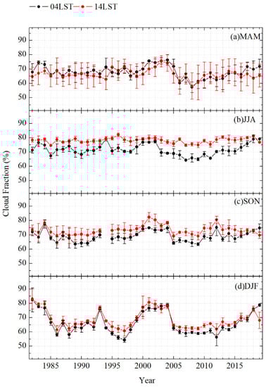
Figure 3.
Time series of seasonal CF over the seas in Arctic (60~90° N) from 1982 to 2019 at 04:00 LST (black) and 14:00 LST (red). (a–d) MAM-DJF. Bars represent ± standard deviation of the mean in each year.

Table 1.
Seasonal mean and standard deviation of CF over the seas in Arctic (60°~90°N) at 04:00 LST and 14:00 LST during 1982–2019.
Table 2.
Results derived by the Mann–Kendall and Sen’s slope statistical tests for seasonal CF for periods of 1982–2007 and 2008–2019.
Figure 4 shows the time series of seasonal ULF (a,c,e,g) and DLF (b,d,f,h) over the Arctic seas. Generally, the variation patterns of ULF or DLF are similar at either 04:00 LST or 14:00 LST, especially in SON and DJF. The difference between 04:00 LST and 14:00 LST is higher in JJA. The simultaneous variations in winter between 04:00 LST and 14:00 LST are probably due to the little impact from solar energy in polar night. Unlike CF variability, both of the ULF and DLF indicate apparent positive trends in all seasons since 1982 according to the results (Table 3) derived by Mann–Kendall and Sen’s slope tests during the period of 1982–2019. Notably, all tests passed 99% significance level, and the ULF shows a more distinct positive trend than the DLF. The increase of DLF and ULF is relatively more pronounced in SON and DJF with higher β values.
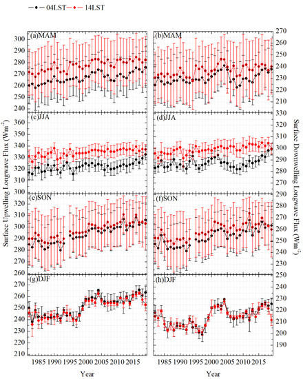
Figure 4.
Time series of seasonal ULF (a,c,e,g) and DLF (b,d,f,h) over the seas in Arctic (60°~90°N) from 1982 to 2019 at 04:00 LST and 14:00 LST. (a,b) MAM, (c,d) JJA, (e,f) SON, and (g,h) DJF. Bars represent ± standard deviation of the mean in each year.
Table 3.
Results derived by the Mann–Kendall and Sen’s slope statistical tests for seasonal DLF and ULF during 1982–2019.
3.2. Spatial Trends
The spatial distributions of CF, DLF, and ULF trends from 1982 to 2019 at 04:00 LST are shown in Figure 5. The trends are expressed by Zs derived by the Mann–Kendall test. Results at 04:00 LST and 14:00 LST (as Supplementary Materials) are similar. According to Figure 5, summer is the season with the least obvious CF changes. The positive trend (significance level of 95%) seems to dominate in the Kara and Barents Seas in all seasons, although it appears weaker in JJA. In the Greenland Sea, the CF shows a nearly consistent negative trend in all seasons, which is more significant in winter. For the Chukchi and Beaufort Seas, the CF trends differ between seasons. A significant negative trend over the Beaufort Sea appears only in MAM, while a significant positive trend over the Chukchi Sea occurs only in SON. For the CF over the Baffin Bay, the trend changed from negative (in spring) to positive (in autumn).
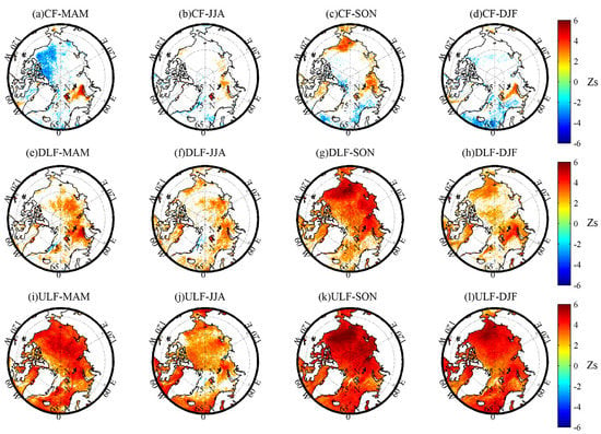
Figure 5.
Spatial distributions of Zs derived by the Mann–Kendall test over the seas in Arctic (60°~90°N) for different seasons from 1982 to 2019 at 04:00 LST. (a–d) CF in MAM, JJA, SON, and DJF. (e–h) DLF in MAM, JJA, SON, and DJF. (i–l) ULF in MAM, JJA, SON, and DJF. The colored regions are at a significance level of 95%.
Different from the spatial distributions of seasonal CF trend, the positive trends of the DLF and ULF are very obvious almost over the entire Arctic seas for all seasons. Moreover, the positive trends for both ULF and DLF are more significant in autumn and relatively weaker in summer. Compared with the DLF, the ULF has a more significant positive trend. The spatial distribution of the trend in spring here is similar as the findings from Huang et al. [27]. They found that for the regions between the central Arctic Ocean and the coasts of Russia, the DLF increased every year from March to mid-May from 2000 to 2015 [27]. Moreover, the ULF showed similar spatial variations as DLF.
Note that the CF, DLF, and ULF have the similar trend in some regions and certain seasons. For example, over the regions close to the eastern coast of Greenland, the CF and DLF present a relatively clear negative trend in MAM and JJA. Over the Baffin Bay, Chukchi Sea, and Kara Sea, the CF, DLF, and ULF display a significant positive trend in SON. Additionally, in other seasons and regions, the CF, DLF, and ULF have the opposite trends. For example, during MAM, over the Chukchi and Beaufort Seas, the CF and DLF present a negative or slightly positive trend, while the ULF shows a strong positive trend.
The results derived by the Sen’s slope statistical test are displayed in Figure 6. The value of β indicates the magnitude of the trends. The dataset is the same as Figure 5. In general, the variation magnitude of CF is small. Only for some regions in the particular season, the trends are relatively significant. For example, the positive magnitudes of the CF over the Kara and Barents Seas are relatively larger in MAM and DJF than those in JJA and SON. Compared with Figure 5, the areas with positive CF trend also show a higher magnitude in SON, such as the East Siberian, Chukchi, and Beaufort Seas. For the DLF and ULF, autumn is the season with the highest β value. It could be noticed that the β values vary regionally and seasonally. The values of positive β are higher over the Kara and Barents Seas for the seasons except JJA. For the East Siberian, Chukchi, and Beaufort Seas, the values of positive β are relatively larger during SON. Negative β values could also be detected over the regions close to the eastern coast of Greenland during MAM and JJA, while with a relatively smaller magnitude.
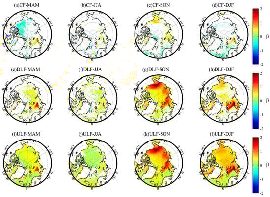
Figure 6.
Spatial distributions of β derived by the Sen’s slope test over the seas in Arctic (60°~90°N) for different seasons from 1982 to 2019 at 04:00 LST. (a–d) CF in MAM, JJA, SON, and DJF. (e–h) DLF in MAM, JJA, SON, and DJF. (i–l) ULF in MAM, JJA, SON, and DJF. The colored regions are at a significance level of 95%.
3.3. Correlations with Sea Ice
Here, the Mann–Kendall test is also applied for the SIC over the seas in Arctic from 60° N to 90° N from 1987 to 2019. Figure 7 shows the spatial distributions of Zs for the SIC of different seasons. Note that the decline of the SIC is most significant during SON over the period of 1987–2019. The prominent retreat of sea ice occurs primarily along the Siberian coast from the Beaufort Sea to the Kara and Barents Seas.
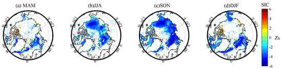
Figure 7.
Spatial distributions of Zs derived by the Mann–Kendall test for the SIC over the seas in Arctic (60°~90°N) for different seasons (a–d) MAM-DJF from 1987 to 2019. The colored regions are at a significance level of 95%.
The surface energy budget, determining the growth or melting of sea ice, is significantly influenced by the radiative effect of clouds [56,57,58]. Considering the significant negative trend of the SIC during SON, the Pearson’s correlation coefficient R between the autumn SIC and the CF, DLF, ULF of each season are examined. Figure 8 shows the results at 04:00 LST from 1987 to 2019. The results at 14:00 LST (as Supplementary Materials) are similar as those at 04:00 LST. The R (statistically significant p < 0.05) is shown in Figure 8. The results of Figure 8 reveal that the correlations between the CF and autumn SIC over the rapid sea-ice retreat areas could be classified into two patterns. One pattern occurs primarily over the Kara and Barents Seas and the Greenland Sea, where there is a particularly pronounced negative linear correlation between the CF and autumn SIC during SON and DJF. Then it turns to slightly negative during MAM and JJA. The result is similar as Wu and Lee [36] that were based on the observations from the Cloud-Aerosol Lidar with Orthogonal Polarization (CALIOP) during 2006–2010 and the Multi-angle Imaging SpectroRadiometer (MISR) during 2000–2010. They found that the enhanced warming of the surface air temperature in the autumn could be caused by the increase in October cloud amount and may result in a positive feedback on the decline of Arctic sea ice [36]. The second pattern is primarily over the Chukchi, Beaufort Seas, and Canadian archipelago. It shows a negative correlation during SON, whereas during MAM, the CF is positively correlated with autumn SIC, and there is no statistically significant relationship for other seasons. The second pattern reveals that for these regions, the decrease of CF in MAM could probably result in the sea ice declining in SON. Huang et al. [27] also found this phenomenon. They proposed that the areas that showed the positive correlation between the CF and September SIC during spring, are either primarily affected by atmospheric circulation or ocean currents or have considerably higher SIC with little variations of sea ice (such as Canadian archipelago) [27].
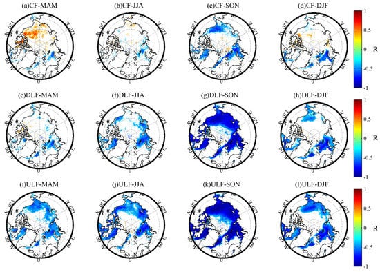
Figure 8.
Seasonal distributions of Pearson’s correlation coefficient R (with p < 0.05) between the autumn SIC and (a–d) CF, (e–h) DLF, (i–l) ULF over the seas in Arctic (60°~90°N) from 1987 to 2019 at 04:00 LST. (a,e,i) MAM; (b,f,j) JJA; (c,g,k) SON; (d,h,l) DJF.
As a whole, the DLF of each season are negatively correlated with autumn SIC. Moreover, the negative correlation between the DLF and autumn SIC is significant during SON. The correlation between the ULF and autumn SIC shows similar spatial distribution. It means that the positive anomalies in DLF could be an important driver for the complex feedback mechanism that triggers sea ice loss. The loss of sea ice might lead to more open water areas with warmer surface, and thus result in higher ULF. Comparing the CF, DLF, and ULF, it reveals that during SON, the negative correlation between the CF and autumn SIC is not as strong as that between the DLF (ULF) and autumn SIC. It suggests that although cloud cover is an important factor affecting surface longwave radiation, it is not only limited to cloud cover. Studies have shown that cloud properties (cloud thickness, cloud height, and cloud phase) are also important for analyzing the relationships with sea ice changes [23,59,60,61].
4. Discussion
Our work is focused on investigating the long-term seasonal variations and trends in cloud fraction and surface longwave radiation over the Arctic seas north of 60° N and further analyzing the potential correlations with the sea ice concentration in autumn. We employed non-parametric Mann–Kendall and Sen’s slope statistical tests into the trend analysis and proposed an inter-comparison between seasons. A linear correlation analysis suggested that there is a significant negative correlation between cloud fraction (surface downwelling/upwelling longwave fluxes) and sea ice concentration during autumn, which is largest in magnitude for regions with substantial sea ice retreat. However, limited to the analyzing method and dataset we used in this study, further work needs to be considered to improve and support our results. Several points should be noted or be further discussed are presented as follows:
- (1)
- It could be noted that the analysis of the surface shortwave radiation is not included in this study. One of the main reasons is that our study focuses not only on the long-term seasonal variations and trends of Arctic clouds and radiation but also on the inter-comparisons between seasons. Considering that a large number of shortwave radiation data are invalid during the polar night in Arctic winter, it is difficult to form a complete analysis of seasonal variations and inter-comparisons between seasons. Additionally, the sea-ice loss or the rapid warming of the Arctic region occurs primarily during the non-melting season in Arctic when the sun’s altitude is extremely low. During this period, the atmospheric downward longwave radiation dominated by the greenhouse effect of atmospheric water vapor and clouds plays a key role in the Arctic surface radiation budget. Therefore, we chose clouds and longwave radiation as the study objects. It is well known that in the surface radiation budget, clouds participate in two main ways: warming the surface through the emission of longwave radiation and cooling the surface by shading the incident shortwave radiation. Adding shortwave radiation analysis would be helpful in interpreting the interactions between clouds, radiation, and sea ice. However, according to some studies [38,62,63], the accuracy of the shortwave radiation products from remote sensing is relatively low in the Arctic. Moreover, seasonal shortwave differences are obtained between satellite estimations and ground-based observations [63]. Improving the accuracy of Arctic shortwave radiation retrieval algorithm and establishing high-quality long-term datasets would be beneficial to the Arctic climate research.
- (2)
- Arctic sea-ice variability is an important indicator of the climate change. The mechanisms and interactions that lead to the Arctic sea-ice loss, which include lots of physical parameters and processes (e.g., clouds, radiation, sea ice, atmospheric circulation, ocean currents, sea-ice motion, and so on), are complicated and the related field is still an open question and difficult to be fully evaluated and analyzed based on literatures. For example, through analysis of CALIPSO Data, Taylor et al. [64] pointed out that the roles of clouds and sea ice in the Arctic climate system might be more complex than the previous assumptions. The increase of autumn cloud cover might delay or slow down the sea ice to refreeze. Thus, it could lead to thinner sea ice or make the sea ice be more likely to be influenced. When it turns to spring and summer, the sea ice might melt even faster. The decrease of sea ice could further lead to more frequent occurrence of low clouds with higher liquid water content. A recent study by Philipp et al. [65] presented that statistically significant anti-correlations between sea ice concentration and low-level cloud fraction are observed in October and November over melting zones using satellite observations of 34 years. They found that the interaction between sea ice concentration and low-level cloud fraction works through two-way feedback. Another study by Vavrus et al. [66] proposed that the loss of sea ice enhanced evaporation within the Arctic, which would influence the initiation of the low-level clouds locally. However, for the increase of the mid- or high- level clouds, the greater meridional moisture transport from lower latitudes could be a major driven factor. Based on the conclusions from the above literatures, the variations of the cloud fraction are not only related to the change of the atmospheric environment caused by the change of sea ice locally but also to the moisture transport caused by the atmospheric circulation remotely. Moreover, the interactions are closely related to the height level information of the clouds. It is difficult to give a reliable conclusion on which physical parameter or physical process plays a leading role in the variations of the Arctic cloud fraction only by relying on observation data analysis in this study. Further work should be done combined with models and multiple kinds of observations, in order to obtain more reliable and accurate analysis on the cloud-sea ice-radiation interactions.
- (3)
- The correlation analysis between autumnal sea ice and seasonal clouds/radiation in this study is based on the Pearson’s correlation coefficient. Additionally, the analysis is within the seasons of the same year, e.g., the correlations between clouds in spring or other seasons and sea ice in autumn of the same year. The correlation result here could only indicate that there is a significant negative correlation between cloud fraction and sea ice concentration during autumn but without supporting information about specific causal links between theses parameters. Some studies have revealed that the interactions between clouds/radiation and sea ice are more likely to occur on a smaller time scale. For example, Cox et al. [67] found that the net cloud radiative forcing from April to May measured at Barrow (1993–2014) is significantly negatively correlated with the sea ice extent of the following September. Huang et al. [27] found that the time period, which the cloud/radiation has significant impact on the September sea ice loss, is primarily during 31 March to 29 April. It would be better to carry out a lag-correlation analysis to investigate the causal relationships not on a seasonal scale but on a monthly or even daily scale. Moreover, Philipp et al. [65] in a recent study firstly employed Granger causality (GC) method (accepted in economics) for the analysis of Arctic sea ice and clouds. They found that a causal two-way interaction between sea ice concentration and low-level cloud fraction, with the impact of sea ice concentration on low-level cloud fraction to be likely stronger than the reverse. More advanced methods of analysis should be adopted in future works, which will provide quantitative assessment of the impact parameters.
- (4)
- The stability is an important indicator for the availability of the long-term dataset. Due to the influence of various factors such as satellite replacement, payload performance, orbit drift and so on, the stability and uncertainties of the long-term series satellite dataset are faced with challenges. The APP-x climate data record of version 2.0 used for the analysis here is a thematic climate data record derived from NOAA/AVHRR. According to the algorithm theoretical basis document of APP-x version 2.0 [41], it reprocessed the entire data record (since 1982) with the latest calibration coefficients of May 2018 for improving the consistency and stability of the dataset. The inter-satellite differences have also been considered in the calibration method. In particular, the cloud fraction and the surface radiative longwave fluxes used here are considered to be of CDR quality. Although the APP-x dataset has been applied for Arctic long-term climate analysis, e.g., [24,25,31,39], it might bring some unavoidable biases. Affected by the complex Arctic environment, such as snow/ice surface and temperature inverse, the accuracy of the retrieval products by passive optical remote sensing still needs to be improved. Although the long-term dataset used here has been revised to minimize the biases, there might be some deviations, which could affect our results.
5. Conclusions
Based on the temporal and spatial analysis derived primarily by the Mann–Kendall and Sen’s slope statistical tests, the APP-x climate data record was used to analyze the long-term seasonal trends and variations of CF, DLF, and ULF over the Arctic seas from 1982 to 2019. The potential correlations between them and the autumn sea-ice retreat were also discussed to examine the inter-seasonal influences. The main conclusions have been drawn as follows:
- (1)
- On the temporal scale, the inter-annual average CF in spring, summer, and autumn maintains a relatively stable level. The changes of inter-annual CF in winter present a fluctuating pattern. A positive trend in CF has been found in each season over the period of 2008 to 2019, while no obvious trend has been found from 1982 to 2007. Significant positive trends in DLF and ULF have been found since 1982. The ULF shows more distinct positive trend than the DLF. The increase of DLF and ULF is relatively more obvious in autumn and winter.
- (2)
- On the spatial scale, the trends in CF are different between seasons. Over the Kara and Barents Seas, the CF maintains a positive trend in each season. Over the Chukchi and Beaufort Seas, the CF presents a negative trend in spring and a pronounced positive trend in autumn. For DLF and ULF, the areas with significant positive trends get to the maximum in autumn. Over the Kara and Barents Seas, the positive trend in DLF or ULF is pronounced in each season except summer. Over the East Siberian, Chukchi, and Beaufort Seas, the positive trend in DLF or ULF is relatively more significant in autumn.
- (3)
- The correlations between the autumn SIC and CF, DLF, ULF in each season of the same year were evaluated. Both DLF and ULF are negatively correlated with autumn SIC in each season, and the negative relationship is more pronounced during autumn. The correlation between CF and autumn SIC is not as strong as that between DLF (ULF) and SIC. During autumn, significant negative correlations between CF and SIC have been found over the regions with prominent retreat of sea ice. In spring, a positive correlation between CF and autumn SIC occurs over the Chukchi, Beaufort Seas, and Canadian archipelago.
Through inter-seasonal comparisons, it suggests that there is a strong negative relationship in autumn between cloud fraction and Arctic sea ice coverage, especially for the regions with rapid sea-ice retreat. There is a complex correlation between clouds, radiation, and sea ice. Changes in cloud cover would cause DLF anomalies, which affect the changes of sea ice further. However, cloud cover is not the only factor that affects the radiation anomalies and sea-ice variations. Other important physical parameters, such as cloud related characteristics, sea-ice thickness, sea-ice motion, snow cover change, changes in precipitation amount and phase, atmospheric circulation, ocean currents, atmospheric environment, and so on, are all of great significance for understanding cloud-radiation process and the related climate feedbacks. Satellite observation is one of the important data in the Arctic region. Due to the limitations of its observation capabilities and retrieval algorithms, there are errors and uncertainties in the obtained cloud and radiation parameters. In order to better interpret the complex mechanism of the Arctic sea ice loss and get more precise seasonal sea ice forecasts, further evaluation and analysis from models and in situ observations are needed.
Supplementary Materials
The following are available online at https://www.mdpi.com/article/10.3390/rs13163201/s1. Figure S1: Spatial distributions of Zs derived by the Mann-Kendall test over the seas in Arctic (60° N~90° N) for different seasons from 1982 to 2019 at 14:00 LST. (a–d) CF in MAM, JJA, SON, and DJF. (e–h) DLF in MAM, JJA, SON, and DJF. (i–l) ULF in MAM, JJA, SON, and DJF. The colored regions are at a significance level of 95%. Figure S2: Spatial distributions of β derived by the Sen’s slope test over the seas in Arctic (60°~90° N) for different seasons from 1982 to 2019 at 14:00 LST. (a–d) CF in MAM, JJA, SON, and DJF. (e–h) DLF in MAM, JJA, SON, and DJF. (i–l) ULF in MAM, JJA, SON, and DJF. The colored regions are at a significance level of 95%. Figure S3: Seasonal distributions of Pearson’s correlation coefficient R (with p < 0.05) between the autumn SIC and (a–d) CF, (e–h) DLF, (i–l) ULF over the seas in Arctic (60° N~90° N) from 1987 to 2019 at 14:00 LST. (a,e,i) MAM; (b,f,j) JJA; (c,g,k) SON; (d,h,l) DJF.
Author Contributions
Conceptualization, J.L.; methodology, J.L.; software, X.W. and B.Y.; validation, Y.B.; formal analysis, X.W. and Y.B.; investigation, G.P.P.; resources, J.L.; data curation, X.W., B.Y. and H.L. and B.H.; writing—original draft preparation, X.W.; writing—review and editing, G.P.P.; visualization, J.L.; supervision, J.L.; project administration, J.L.; funding acquisition, J.L. All authors have read and agreed to the published version of the manuscript.
Funding
This research was conducted with funding provided by the National Key R&D Program of China (2018 YFC1407200, 2018YFC1407204) and National Natural Science Foundation of China (61531019).
Institutional Review Board Statement
Not applicable.
Informed Consent Statement
Not applicable.
Data Availability Statement
Please refer to App-x Data Availability Statements at https://www.ncei.noaa.gov/access/metadata/landing-page/bin/iso?id=gov.noaa.ncdc:C00941, accessed on 1 February 2020 to 30 December 2020. Refer to Sea Ice Concentration Data Availability Statements in section “Use and Copyright” at https://nsidc.org/about/use_copyright.html, accessed on 23 July 2020.
Acknowledgments
Authors wish to thank the NOAA National Centers for Environmental Information (NCEI) for the NOAA Climate Data Record (CDR) of AVHRR Polar Pathfinder Extended (APP-X) dataset. In addition, all authors wish to thank the National Snow and Ice Data Center (NSIDC) for providing the sea ice concentration data and the Masks and Overlays data. George P. Petropoulos’s participation in this study was funded under the European Union’s Horizon 2020 Marie Skłodowska-Curie “ENVISION-EO” project (grant agreement No 752094). Thanks to the anonymous reviewers for their valuable suggestions regarding this paper.
Conflicts of Interest
The authors declare no conflict of interest.
References
- Wang, Y.; Bi, H.; Huang, H.; Liu, Y.; Liu, Y.; Liang, X.; Fu, M.; Zhang, Z. Satellite-observed trends in the Arctic sea ice concentration for the period 1979–2016. J. Oceanol. Limnol. 2019, 37, 18–37. [Google Scholar] [CrossRef]
- Zhan, Y.; Davies, R. September Arctic sea ice extent indicated by June reflected solar radiation. J. Geophys. Res. Atmos. 2017, 122, 2194–2202. [Google Scholar] [CrossRef]
- Parkinson, C.L.; DiGirolamo, N.E. New visualizations highlight new information on the contrasting Arctic and Antarctic sea-ice trends since the late 1970s. Remote Sens. Environ. 2016, 183, 198–204. [Google Scholar] [CrossRef]
- Petty, A.A.; Stroeve, J.C.; Holland, P.R.; Boisvert, L.N.; Bliss, A.C.; Kimura, N.; Meier, W.N. The Arctic sea ice cover of 2016: A year of record-low highs and higher-than-expected lows. Cryosphere 2018, 12, 433–452. [Google Scholar] [CrossRef]
- Bliss, A.C.; Steele, M.; Peng, G.; Meier, W.N.; Dickinson, S. Regional variability of Arctic sea ice seasonal change climate indicators from a passive microwave climate data record. Environ. Res. Lett. 2019, 14, 045003. [Google Scholar] [CrossRef]
- Kumar, A.; Yadav, J.; Mohan, R. Global warming leading to alarming recession of the Arctic sea-ice cover: Insights from remote sensing observations and model reanalysis. Heliyon 2020, 6, e04355. [Google Scholar] [CrossRef]
- Desmarais, A.l.; Tremblay, L.B. Assessment of Decadal Variability in Sea Ice in the Community Earth System Model against a Long-Term Regional Observational Record: Implications for the Predictability of an Ice-Free Arctic. J. Clim. 2021, 34, 5367–5384. [Google Scholar] [CrossRef]
- Kay, J.E.; L’Ecuyer, T.; Gettelman, A.; Stephens, G.; O’Dell, C. The contribution of cloud and radiation anomalies to the 2007 Arctic sea ice extent minimum. Geophys. Res. Lett. 2008, 35. [Google Scholar] [CrossRef]
- Eastman, R.; Warren, S.G. Arctic Cloud Changes from Surface and Satellite Observations. J. Clim. 2010, 23, 4233–4242. [Google Scholar] [CrossRef]
- Kapsch, M.-L.; Graversen, R.G.; Tjernström, M.; Bintanja, R. The Effect of Downwelling Longwave and Shortwave Radiation on Arctic Summer Sea Ice. J. Clim. 2016, 29, 1143–1159. [Google Scholar] [CrossRef]
- Boccolari, M.; Parmiggiani, F. Trends and variability of cloud fraction cover in the Arctic, 1982–2009. Theor. Appl. Climatol. 2018, 132, 739–749. [Google Scholar] [CrossRef]
- Curry, J.A.; Ebert, E.E. Annual Cycle of Radiation Fluxes over the Arctic Ocean: Sensitivity to Cloud Optical Properties. J. Clim. 1992, 5, 1267–1280. [Google Scholar] [CrossRef]
- Curry, J.A.; Schramm, J.L.; Ebert, E.E. Impact of clouds on the surface radiation balance of the Arctic Ocean. Meteorol. Atmos. Phys. 1993, 51, 197–217. [Google Scholar] [CrossRef]
- Curry, J.A.; Schramm, J.L.; Rossow, W.B.; Randall, D. Overview of Arctic Cloud and Radiation Characteristics. J. Clim. 1996, 9, 1731–1764. [Google Scholar] [CrossRef]
- Liu, Y.; Key, J.R.; Liu, Z.; Wang, X.; Vavrus, S.J. A cloudier Arctic expected with diminishing sea ice. Geophys. Res. Lett. 2012, 39. [Google Scholar] [CrossRef]
- Palm, S.P.; Strey, S.T.; Spinhirne, J.; Markus, T. Influence of Arctic sea ice extent on polar cloud fraction and vertical structure and implications for regional climate. J. Geophys. Res. Atmos. 2010, 115. [Google Scholar] [CrossRef]
- Shupe, M.D.; Intrieri, J.M. Cloud Radiative Forcing of the Arctic Surface: The Influence of Cloud Properties, Surface Albedo, and Solar Zenith Angle. J. Clim. 2004, 17, 616–628. [Google Scholar] [CrossRef]
- Intrieri, J.M.; Fairall, C.W.; Shupe, M.D.; Persson, P.O.G.; Andreas, E.L.; Guest, P.S.; Moritz, R.E. An annual cycle of Arctic surface cloud forcing at SHEBA. J. Geophys. Res. Ocean. 2002, 107, SHE 13-1–SHE 13-14. [Google Scholar] [CrossRef]
- Huang, Y.; Dong, X.; Xi, B.; Dolinar, E.K.; Stanfield, R.E.; Qiu, S. Quantifying the Uncertainties of Reanalyzed Arctic Cloud and Radiation Properties Using Satellite Surface Observations. J. Clim. 2017, 30, 8007–8029. [Google Scholar] [CrossRef]
- Chernokulsky, A.; Mokhov, I. Climatology of Total Cloudiness in the Arctic: An Intercomparison of Observations and Reanalyses. Adv. Meteorol. 2012, 2012, 542093. [Google Scholar] [CrossRef]
- Zygmuntowska, M.; Mauritsen, T.; Quaas, J.; Kaleschke, L. Arctic Clouds and Surface Radiation—A critical comparison of satellite retrievals and the ERA-Interim reanalysis. Atmos. Chem. Phys. 2012, 12, 6667–6677. [Google Scholar] [CrossRef]
- Schweiger, A.J.; Key, J.R. Arctic Cloudiness. Comparison of ISCCP-C2 and Nimbus-7 Satellite-derived Cloud Products with a Surface-based Cloud Climatology. J. Clim. 1992, 5, 1514–1527. [Google Scholar] [CrossRef]
- Eastman, R.; Warren, S.G. Interannual Variations of Arctic Cloud Types in Relation to Sea Ice. J. Clim. 2010, 23, 4216–4232. [Google Scholar] [CrossRef]
- Schweiger, A.J. Changes in seasonal cloud cover over the Arctic seas from satellite and surface observations. Geophys. Res. Lett. 2004, 31. [Google Scholar] [CrossRef]
- Wang, X.; Key, J.R. Arctic Surface, Cloud, and Radiation Properties Based on the AVHRR Polar Pathfinder Dataset. Part II: Recent Trends. J. Clim. 2005, 18, 2575–2593. [Google Scholar] [CrossRef]
- Comiso, J.C. Warming Trends in the Arctic from Clear Sky Satellite Observations. J. Clim. 2003, 16, 3498–3510. [Google Scholar] [CrossRef]
- Huang, Y.; Dong, X.; Xi, B.; Dolinar, E.K.; Stanfield, R.E. The footprints of 16 year trends of Arctic springtime cloud and radiation properties on September sea ice retreat. J. Geophys. Res. Atmos. 2017, 122, 2179–2193. [Google Scholar] [CrossRef]
- Wielicki, B.A.; Barkstrom, B.R.; Harrison, E.F.; Lee, R.B.; Smith, G.L.; Cooper, J.E. Clouds and the Earth’s Radiant Energy System (CERES): An Earth Observing System Experiment. Bull. Am. Meteorol. Soc. 1996, 77, 853–868. [Google Scholar] [CrossRef]
- Schweiger, A.J.; Key, J.R. Arctic Ocean Radiative Fluxes and Cloud Forcing Estimated from the ISCCP C2 Cloud Dataset, 1983–1990. J. Appl. Meteorol. 1994, 33, 948–963. [Google Scholar] [CrossRef]
- Walsh, J.E.; Chapman, W.L. Arctic Cloud–Radiation–Temperature Associations in Observational Data and Atmospheric Reanalyses. J. Clim. 1998, 11, 3030–3045. [Google Scholar] [CrossRef]
- Wang, X.; Key, J.R. Recent Trends in Arctic Surface, Cloud, and Radiation Properties from Space. Science 2003, 299, 1725. [Google Scholar] [CrossRef]
- Vavrus, S. The Impact of Cloud Feedbacks on Arctic Climate under Greenhouse Forcing. J. Clim. 2004, 17, 603–615. [Google Scholar] [CrossRef]
- Dong, X.; Xi, B.; Crosby, K.; Long, C.N.; Stone, R.S.; Shupe, M.D. A 10 year climatology of Arctic cloud fraction and radiative forcing at Barrow, Alaska. J. Geophys. Res. Atmos. 2010, 115. [Google Scholar] [CrossRef]
- Kapsch, M.-L.; Graversen, R.G.; Tjernström, M. Springtime atmospheric energy transport and the control of Arctic summer sea-ice extent. Nat. Clim. Chang. 2013, 3, 744–748. [Google Scholar] [CrossRef]
- Schweiger, A.J.; Lindsay, R.W.; Vavrus, S.; Francis, J.A. Relationships between Arctic Sea Ice and Clouds during Autumn. J. Clim. 2008, 21, 4799–4810. [Google Scholar] [CrossRef]
- Wu, D.L.; Lee, J.N. Arctic low cloud changes as observed by MISR and CALIOP: Implication for the enhanced autumnal warming and sea ice loss. J. Geophys. Res. Atmos. 2012, 117. [Google Scholar] [CrossRef]
- Jun, S.-Y.; Ho, C.-H.; Jeong, J.-H.; Choi, Y.-S.; Kim, B.-M. Recent changes in winter Arctic clouds and their relationships with sea ice and atmospheric conditions. Tellus A Dyn. Meteorol. Oceanogr. 2016, 68, 29130. [Google Scholar] [CrossRef]
- Key, J. The AVHRR Polar Pathfinder Climate Data Records. Remote Sens. 2016, 8, 167. [Google Scholar] [CrossRef]
- Wang, X.; Key, J.R. Arctic Surface, Cloud, and Radiation Properties Based on the AVHRR Polar Pathfinder Dataset. Part I: Spatial and Temporal Characteristics. J. Clim. 2005, 18, 2558–2574. [Google Scholar] [CrossRef]
- Key, J.; Lui, Y.; Wang, X. NOAA CDR Program (2019): NOAA Climate Data Record (CDR) of AVHRR Polar Pathfinder (APP) Cryosphere, Version 2.0. 2019. Available online: https://www.ncei.noaa.gov/access/metadata/landing-page/bin/iso?id=gov.noaa.ncdc:C01579 (accessed on 15 January 2020).
- Key, J.; Wang, X. Climate Algorithm Theoretical Basis Document (C-ATBD) Extended AVHRR Polar Pathfinder (APP-x). Available online: https://www.ncei.noaa.gov/pub/data/sds/cdr/CDRs/AVHRR_Extended_Polar_Pathfinder/AlgorithmDescription_01B-24b.pdf (accessed on 15 January 2020).
- Key, J.; Wang, X. Climate Algorithm Theoretical Basis Document (C-ATBD) AVHRR Polar Pathfinder (APP). Available online: https://www.ncei.noaa.gov/pub/data/sds/cdr/CDRs/AVHRR_Polar_Pathfinder/AlgorithmDescription_01B-24a.pdf (accessed on 15 January 2020).
- Peng, G.; Meier, W.; Scott, D.; Savoie, M. A long-term and reproducible passive microwave sea ice concentration data record for climate studies and monitoring. Earth Syst. Sci. Data 2013, 5, 311–318. [Google Scholar] [CrossRef]
- Meier, W.N.; Fetterer, F.; Savoie, M.; Mallory, S.; Duerr, R.; Stroeve, J. NOAA/NSIDC Climate Data Record of Passive Microwave Sea Ice Concentration, Version 3. 2017. Available online: https://nsidc.org/data/g02202/versions/3 (accessed on 23 July 2020).
- Meier, W.; Windnagel, A. Climate Algorithm Theoretical Basis Document (C-ATBD) Sea Ice Concentration. Available online: https://nsidc.org/sites/nsidc.org/files/technical-references/SeaIce_CDR_CATBD_final_Rev-7.pdf (accessed on 27 July 2020).
- Windnagel, A. NOAA/NSIDC Climate Data Record of Passive Microwave Sea Ice Concentration, Version 3 USER GUIDE. Available online: https://nsidc.org/sites/nsidc.org/files/G02202-V001-UserGuide.pdf (accessed on 20 July 2021).
- Cavalieri, D.J.; Gloersen, P.; Campbell, W.J. Determination of sea ice parameters with the NIMBUS 7 SMMR. J. Geophys. Res. Atmos. 1984, 89, 5355–5369. [Google Scholar] [CrossRef]
- Comiso, J.C. Characteristics of Arctic winter sea ice from satellite multispectral microwave observations. J. Geophys. Res. Ocean. 1986, 91, 975–994. [Google Scholar] [CrossRef]
- Kern, S.; Lavergne, T.; Notz, D.; Pedersen, L.T.; Tonboe, R.T.; Saldo, R.; Sørensen, A.M. Satellite passive microwave sea-ice concentration data set intercomparison: Closed ice and ship-based observations. Cryosphere 2019, 13, 3261–3307. [Google Scholar] [CrossRef]
- Kern, S.; Lavergne, T.; Notz, D.; Pedersen, L.T.; Tonboe, R. Satellite passive microwave sea-ice concentration data set inter-comparison for Arctic summer conditions. Cryosphere 2020, 14, 2469–2493. [Google Scholar] [CrossRef]
- Stuart, A. Rank Correlation Methods. By M. G. Kendall, 2nd edition. Br. J. Stat. Psychol. 1956, 9, 68. [Google Scholar] [CrossRef]
- Kamal, N.; Pachauri, S. Mann-Kendall Test—A Novel Approach for Statistical Trend Analysis. Int. J. Comput. Trends Technol. 2018, 63, 18–21. [Google Scholar] [CrossRef]
- Sen, P.K. Estimates of the Regression Coefficient Based on Kendall’s Tau. J. Am. Stat. Assoc. 1968, 63, 1379–1389. [Google Scholar] [CrossRef]
- Gilbert, R.O. Statistical Methods for Environmental Pollution Monitoring; John Wiley & Sons: New York, NY, USA, 1987; p. 336. [Google Scholar]
- Gocic, M.; Trajkovic, S. Analysis of changes in meteorological variables using Mann-Kendall and Sen’s slope estimator statistical tests in Serbia. Glob. Planet. Chang. 2013, 100, 172–182. [Google Scholar] [CrossRef]
- Liu, Y.; Key, J.R.; Wang, X. The Influence of Changes in Cloud Cover on Recent Surface Temperature Trends in the Arctic. J. Clim. 2008, 21, 705–715. [Google Scholar] [CrossRef]
- Tjernström, M.; Sedlar, J.; Shupe, M.D. How Well Do Regional Climate Models Reproduce Radiation and Clouds in the Arctic? An Evaluation of ARCMIP Simulations. J. Appl. Meteorol. Climatol. 2008, 47, 2405–2422. [Google Scholar] [CrossRef]
- Liu, Y.; Key, J.R.; Wang, X. Influence of changes in sea ice concentration and cloud cover on recent Arctic surface temperature trends. Geophys. Res. Lett. 2009, 36. [Google Scholar] [CrossRef]
- Kay, J.E.; Gettelman, A. Cloud influence on and response to seasonal Arctic sea ice loss. J. Geophys. Res. Atmos. 2009, 114. [Google Scholar] [CrossRef]
- Morrison, A.; Kay, J.; Chepfer, H.; Guzman, R.; Yettella, V. Isolating the Liquid Cloud Response to Recent Arctic Sea Ice Variability Using Spaceborne Lidar Observations. J. Geophys. Res. Atmos. 2018, 123, 473–490. [Google Scholar] [CrossRef]
- Sato, K.; Inoue, J.; Kodama, Y.-M.; Overland, J.E. Impact of Arctic sea-ice retreat on the recent change in cloud-base height during autumn. Geophys. Res. Lett. 2012, 39. [Google Scholar] [CrossRef]
- Riihelä, A.; Key, J.R.; Meirink, J.F.; Kuipers Munneke, P.; Palo, T.; Karlsson, K.-G. An intercomparison and validation of satellite-based surface radiative energy flux estimates over the Arctic. J. Geophys. Res. Atmos. 2017, 122, 4829–4848. [Google Scholar] [CrossRef]
- Sun, D.; Ji, C.; Sun, W.; Yang, Y.; Wang, H. Accuracy assessment of three remote sensing shortwave radiation products in the Arctic. Atmos. Res. 2018, 212, 296–308. [Google Scholar] [CrossRef]
- Taylor, P.C.; Kato, S.; Xu, K.-M.; Cai, M. Covariance between Arctic sea ice and clouds within atmospheric state regimes at the satellite footprint level. J. Geophys. Res. Atmos. 2015, 120, 12656–12678. [Google Scholar] [CrossRef]
- Philipp, D.; Stengel, M.; Ahrens, B. Analyzing the Arctic Feedback Mechanism between Sea Ice and Low-Level Clouds Using 34 Years of Satellite Observations. J. Clim. 2020, 33, 7479–7501. [Google Scholar] [CrossRef]
- Vavrus, S.J.; Bhatt, U.S.; Alexeev, V.A. Factors Influencing Simulated Changes in Future Arctic Cloudiness. J. Clim. 2011, 24, 4817–4830. [Google Scholar] [CrossRef]
- Cox, C.J.; Uttal, T.; Long, C.N.; Shupe, M.D.; Stone, R.S.; Starkweather, S. The Role of Springtime Arctic Clouds in Determining Autumn Sea Ice Extent. J. Clim. 2016, 29, 6581–6596. [Google Scholar] [CrossRef]


Publisher’s Note: MDPI stays neutral with regard to jurisdictional claims in published maps and institutional affiliations. |
© 2021 by the authors. Licensee MDPI, Basel, Switzerland. This article is an open access article distributed under the terms and conditions of the Creative Commons Attribution (CC BY) license (https://creativecommons.org/licenses/by/4.0/).