Evaluation of Point Hyperspectral Reflectance and Multivariate Regression Models for Grapevine Water Status Estimation

Abstract

Monitoring and management of plant water status over the critical period between flowering and veraison, plays a significant role in producing grapes of premium quality. Hyperspectral spectroscopy has been widely studied in precision farming, including for the prediction of grapevine water status. However, these studies were presented based on various combinations of transformed spectral data, feature selection methods, and regression models. To evaluate the performance of different modeling pipelines for estimating grapevine water status, a study spanning the critical period was carried out in two commercial vineyards at Martinborough, New Zealand. The modeling used six hyperspectral data groups (raw reflectance, first derivative reflectance, second derivative reflectance, continuum removal variables, simple ratio indices, and vegetation indices), two variable selection methods (Spearman correlation and recursive feature elimination based on cross-validation), an ensemble of selected variables, and three regression models (partial least squares regression, random forest regression, and support vector regression). Stem water potential (used as a proxy for vine water status) was measured by a pressure bomb. Hyperspectral reflectance was undertaken by a handheld spectroradiometer. The results show that the best predictive performance was achieved by applying partial least squares regression to simple ratio indices (R² = 0.85; RMSE = 110 kPa). Models trained with an ensemble of selected variables comprising multicombination of transformed data and variable selection approaches outperformed those fitted using single combinations. Although larger data sizes are needed for further testing, this study compares 38 modeling pipelines and presents the best combination of procedures for estimating vine water status. This may lead to the provision of rapid estimation of vine water status in a nondestructive manner and highlights the possibility of applying hyperspectral data to precision irrigation in vineyards.

1. Introduction

Grapevine (Vitis spp.) is considered one of the most important berry crops in the world, due to its commercial derivative—wine. The market price of this product is defined by the quality of harvested berries, and water management applied during the growing season has a significant effect on this quality [1]. Inadequate water inputs can harm berry quality as the production of some quality-specific flavor precursors is compromised [2]. Excessive irrigation can result in high vigor and strong vegetative growth, further delaying ripening and generating undesirable flavors in the wine [3]. Hence, maintaining grapevine water status (GWS) within a specific range is critical to quality management, and thus, the growers’ profit. Nevertheless, studies have shown vines in a single block exhibit a significant variation of GWS even if they receive the same amount of irrigation [4]. This variability becomes more prominent under nonirrigated conditions commonly encountered in viticulture [5], and this potentially leads to increasing variability in berry composition across the vineyard. Most viticulturists use soil moisture sensors and pressure chambers to characterize the dynamics of GWS throughout different growing stages [6]. These measurements provide viticulturists a reference to help guide management strategies that ensure grape quality. However, soil moisture sensors obtain only localized soil moisture values and often fail to reveal the variability of soil water status at depth and spatially, due to soil heterogeneity [7]. The pressure chamber, despite providing direct information regarding GWS, is destructive, labor-intensive, and time-consuming. Sampling surveys by pressure chambers do not accurately show spatial and temporal variation in moisture conditions across vines, making it challenging to use in irrigation scheduling, unless high-density sampling is undertaken [8]. In this context, remote sensing is a potentially promising method that can be used in a nondestructive and timely manner for GWS optimization.

The theoretical basis of applying remote sensing to assessing GWS is attributed to the interaction between leaf water content and the spectral information contained in visible (VIS), near-infrared (NIR), and shortwave infrared (SWIR) regions of the electromagnetic spectrum [9]. In the VIS spectrum, the reflectance response is a cumulative effect of water deficit on the content of leaf pigments and the process of photosynthesis [10]. In the NIR to SWIR spectrum, a partial response is due to the internal structure of the leaf resulting from reduced water content [11]. The rest of the response originates from four water absorption bands centering at around 970, 1200, 1450, and 1940 nm [12]. The reflectance in the SWIR region is also determined by nitrogen and various forms of carbon (i.e., lignin and cellulose) in leaves [13,14]. The spectral signatures, the variation of reflectance by wavelengths, can be received either by multispectral or by hyperspectral sensors. Hyperspectral data, characterized by thousands of bands around 1 nm bandwidth over 350–2500 nm [15], can provide further insights into the relationship between spectral information and a target parameter of interest. Several successful studies have been reported applying hyperspectral techniques to assessing GWS [15,16,17,18]. To better extract relevant spectral information, it is essential to investigate the full spectrum instead of certain regions [19,20].

Nevertheless, when using full-spectrum hyperspectral data, problems related to high dimensionality and multicollinearity occur. These characteristics may violate some assumptions of statistics, for instance, the assumption of independence between variables [21]. Models trained with such data tend to overfit and become less accurate in prediction capability [22]. Overfitting occurs when the regression model learns the training set too well, but generalizes poorly using the test set. These issues also limit the transferability and interpretability of the models, making it difficult to identify the important relationship between predictors and responses. To minimize this disturbance and enhance the sensitivity of hyperspectral data to target indicators, various preprocessing or transformation approaches have been used to address these issues [23]. These include using specific bands to form new indices (vegetation indices [16]), removing background interference to compare spectral characteristics (continuum removal [24]), or taking the derivative of the reflectance to amplify signals [25]. In addition, variable selection is a method commonly employed to decrease the complexity and the size of the datasets [26]. This process selects a subset of variables that optimally describes the relationship between input data and target indicators. Therefore, subsequent modeling can be improved by avoiding overfitting, and a better generalization is obtained by removing noise and irrelevant variables from the dataset [27]. Another efficient way to decrease complexity is feature extraction which creates an independently new set of variables based on the input variables to minimize the issue of dimensionality [28].

Hyperspectral measurement records reflectance at thousands of wavelengths, and each wavelength-based recording (variable) contains only a fragment of the information available in the entire spectrum. Significant information may be lost if just a few variables are utilized. In the study of Romero et al. [29], the modeling performance was enhanced after taking all variables as inputs instead of using a subset of them. The use of multivariate regression models and machine learning algorithms showed promise in exploiting the full information contained in hyperspectral data and searching the complex patterns between reflectance and crop water status. These methods include partial least squares regression [30], random forest regression [31], and support vector machines [32]. Moreover, it has been recently reported that the advantages of increasing prediction accuracy of hyperspectral-based studies by combining different methods [33]. This ensemble approach has been implemented by combining different algorithms or techniques for modeling [34,35] and for variable selection [36,37]. The performance of the ensemble method was demonstrated to be generally better and more robust than a single method alone.

Some studies have been shown to achieve high accuracies in estimating plant water status, using hyperspectral reflectance [15,30,38,39,40]. However, few studies have compared the accuracy of modeling performance, based on different, pipelines in terms of multicombination of data transformation methods, variable selection approaches, and multivariate regression models. Besides, the ensemble technique, to our knowledge, has never been tested for its potential in the domain of hyperspectral data—GWS estimation. This study aims to (i) evaluate the performance of various modeling pipelines composed of six transformation data groups, two variable selection approaches, and three multivariate regression models; (ii) examine the modeling performance after applying ensemble techniques in terms of using collective variables from different combinations of transformed data groups and variable selection methods as inputs.

2. Materials and Methods

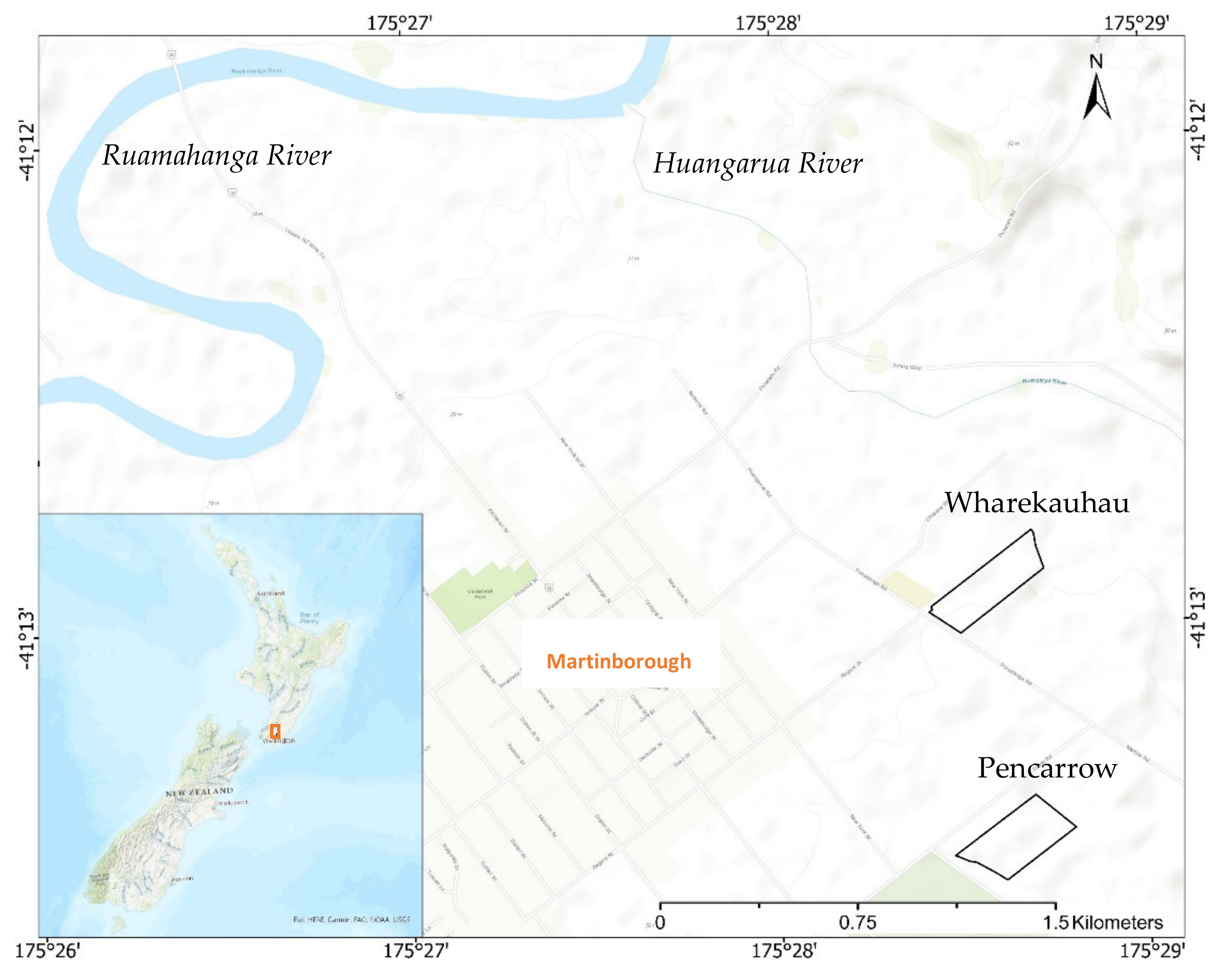
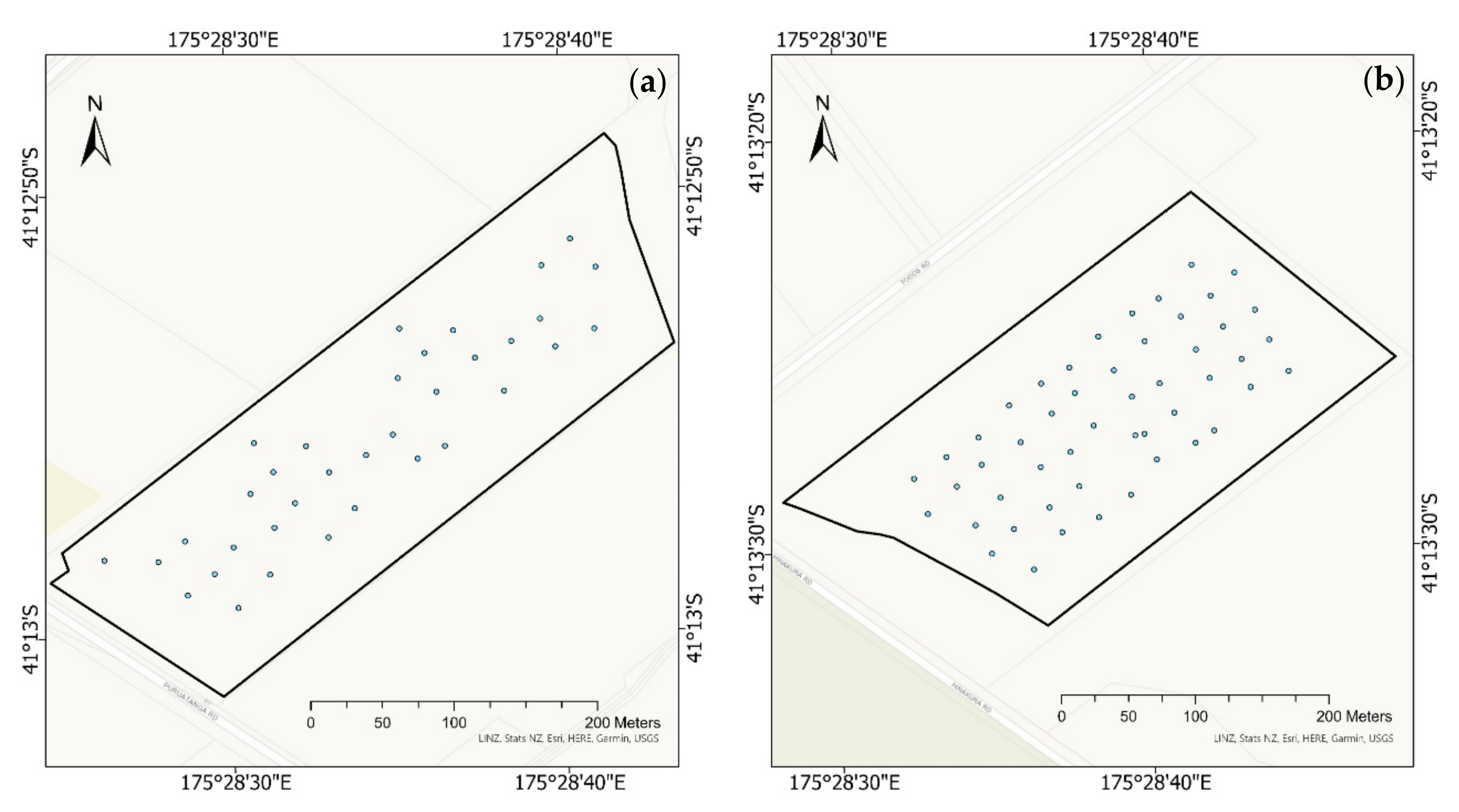
2.1. The Context of the Study Vineyards

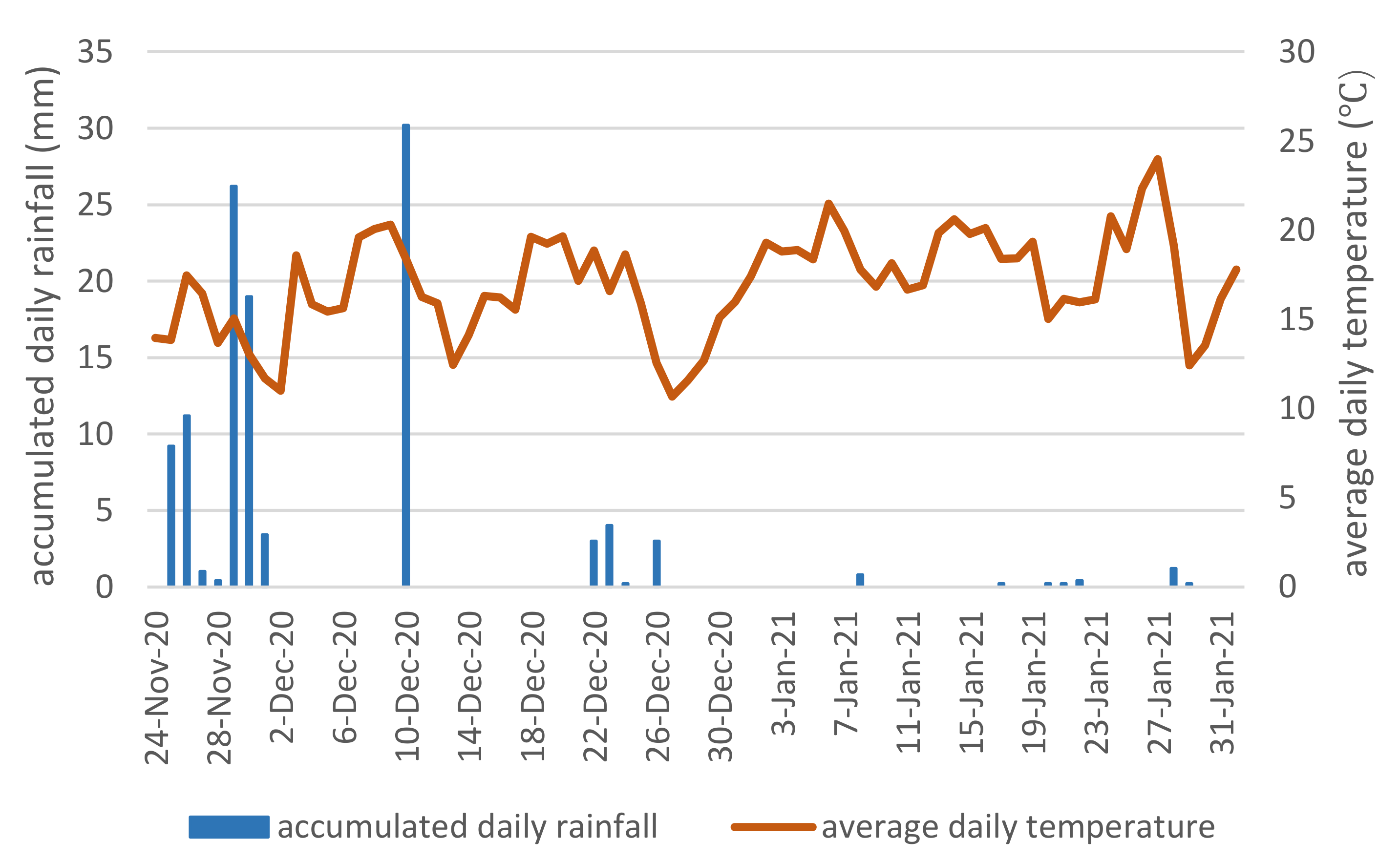
The study vineyards are located at Martinborough in the Greater Wellington Region in New Zealand (NZ). Both vineyards are sited on a complex of young soils overlying gravels, developed from sedimentary alluvium associated with the nearby Ruamahanga and Huangarua Rivers (Figure 1). The vineyards are two commercial vineyards owned by Palliser Estate and are named Wharekauhau and Pencarrow. Our study areas in these two vineyards are 6.6 and 6.7 ha, respectively. Chardonnay, Pinot Noir, and Sauvignon Blanc dominate the cultivars in both vineyards. Among them, Pinot Noir is noteworthy for being flavor-rich under controlled water deficit conditions. However, severe water stress is detrimental to the yield. Accordingly, Pinot Noir was chosen as the target cultivar in this study, due to its requirement for relatively precise irrigation management. The Pinot Noir vines were planted in the vineyards in 1998–2000, grafted on rootstock 101-14, and trained with two-cane vertical shoot positioning. Inter- and intra-row planting space is 2.2 × 1.7 m for Wharekauhau and 2.2 × 1.8 m for Pencarrow. The annual growth cycle of grapevine in NZ comprises budburst, shoot growth, and flowering (September–November), fruit set and veraison (December–February) followed by berry development and harvesting (March–May). Cultivation practices, such as shoot thinning, bud rubbing, and leaf plucking, are regularly conducted from October to December during the growing season. Irrigation is usually not required before flowering. From flowering to veraison, as the management of GWS in this timeframe is the most critical determinant to the final berry quality, irrigation is usually determined using the measurement of a pressure chamber.

2.2. Study Period

The trials reported in this paper took place from late November 2020 to early February 2021 to match the most critical period for GWS management. The measurement dates, that avoided rain days, were 27 November 2020, 4 December 2020, 14 January 2021, and 22 January 2021 at Wharekauhau, and 4 December 2020, 14 January 2021, 22 January 2021, and 1 February 2021 at Pencarrow.

During the study period, the daily mean temperature varied from 10 to 24 °C, and daily accumulated rainfall ranged between 0 and 30 mm at the vineyards (Figure 2). From flowering in late November 2020, several rainfall events occurred in Martinborough, with a maximum daily accumulated rainfall of 30 mm on 10 December. Due to adequate rainfall in late November, the two vineyards were not irrigated in the study period (late November 2020 through to early February 2021) when GWS was a moderate water deficit, desirable for berry quality. At Palliser Estate, the GWS of Pinot Noir during the critical period is expected to keep close to −1300 kPa.

2.3. Measurement of Vine Stem Water Potential

Stem water potential (Ψstem) was chosen as a proxy for GWS. As Ψ refers to the suction or the negative pressure, it is usually lower in plants compared to that in soils to enable the absorption of water. The plants naturally maintain a decreasing gradient of Ψ along different parts of the canopy to preserve constant water flow from roots to leaves, later transpiring through the stomata. Ψstem has been expressed as a comprehensive indicator for early water deficit in vines during the day [41]. On each measurement date, several healthy vines were sampled in grids to account for the variability across the vineyards, with two mature and fully expanded leaves from the middle part of the canopy. The mature and fully expanded leaves are more representative of the status of canopies. A pressure chamber model 610 (MPS, Albany, NY, USA) was employed between the hours of 12:00 and 15:00 to assess Ψstem. Prior to the measurement, the sampled leaves were covered with sealable plastic bags for around 1 h. In this way, transpiration is stopped when the equilibrium of water potential between leaf and stem is attained, which makes this leaf-scale measurement more representative of the canopy conditions. When using the pressure chamber, the pressure is applied onto the scion, which is equal and opposite to the suction in the scion, until the sap is extruded. Therefore, the higher the reading, the more dehydrated the vine is. The two measurements per vine were averaged to represent the canopy water status. A total of 85 separate canopies were surveyed in the two vineyards (Figure 3;

Table 1. The number of surveyed canopies on each measurement date.

	Measurement Data
Vineyard	27 November 2020	4 December 2020	14 January 2021	22 January 2021	1 February 2021
Wharekauhau	11	8	8	8	-
Pencarrow	-	10	11	11	18

).

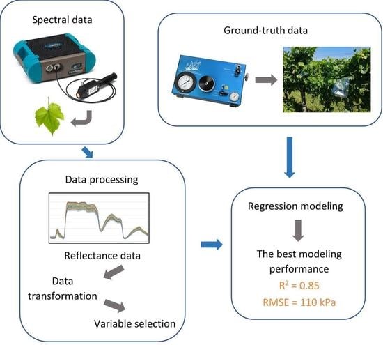
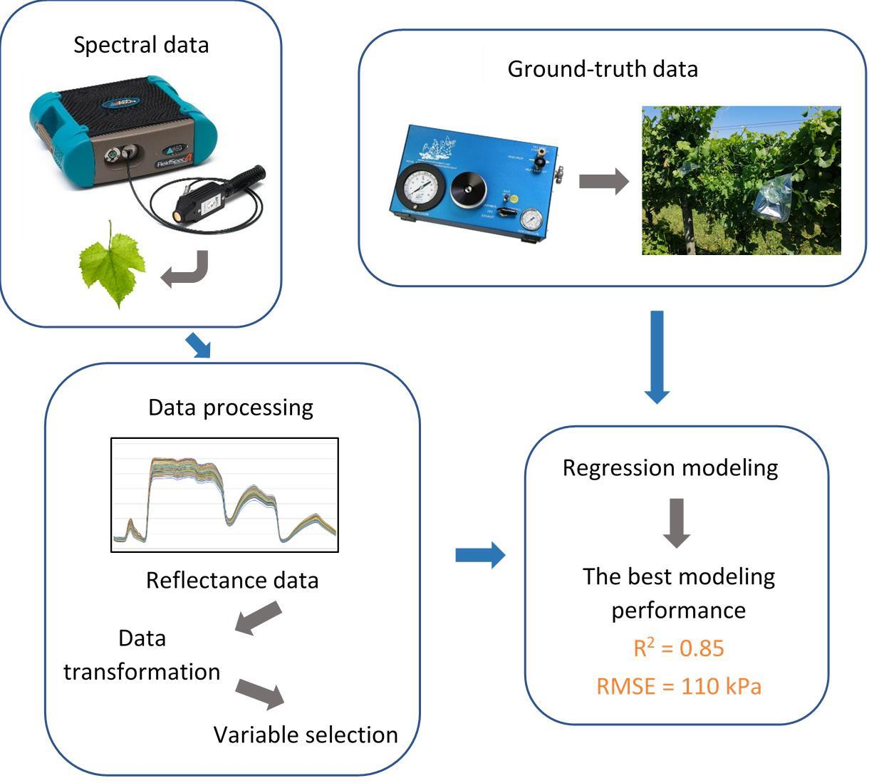
2.4. Acquisition of Spectral Data and Preprocessing

Hyperspectral reflectance data were collected by an ASD FieldSpec 4 Hi-Res NG Spectroradiometer (Malvern Panalytical Ltd., Malvern, UK) equipped with a leaf clip and contact probe (touching the surface of the leaf when measuring), providing controlled illumination throughout the field measurements. A white panel ceramic, referencing tile was used for calibrating and referencing the spectrum during the field survey, which was carried out each time before collecting the reflectance data of the next canopy. The reflectance was calculated as the ratio of the optical energy from a sample to the optical energy from the reference panel. The spectral range covers 350–2500 nm with a sampling interval of 1.4 nm between 350–1000 nm and 1.1 nm between 1001–2500 nm. These intervals were then interpolated to 1 nm, resulting in 2151 values for every spectral measurement.

To ensure comparability, the spectral data were obtained during the same timeframe as Ψstem data measurements. Two leaves per vine, from the same vine used for collecting Ψstem, were selected with similar criteria and positions in the canopies. Measurements were undertaken on the left side and right side of the adaxial surface of each leaf, while avoiding leaf veins, spots, and holes to ensure representative sampling. Five repetitive readings were made at each measuring point, with a total of 20 readings collected per canopy.

Signal instability (noise) was observed at both edges of the electromagnetic spectrum (<400 and >2400 nm), so the reflectance data in these regions were not used for analysis. Each reading was processed using ViewSpec Pro 6.2 software (Analytical Spectral Devices, Inc., Boulder, CO, USA). Splice correction was applied to all the spectra to adjust the mismatches in the visible-near infrared and shortwave infrared two regions. This was achieved by calculating a bias value to help match the shortwave infrared one region at the splice points. These corrected spectra were exported as ASCII text files, and then they were averaged to obtain the mean spectral signatures for the 85 canopies.

2.5. Data Transformation

The raw reflectance (the mean hyperspectral signatures of the 85 canopies) were transformed into five feature groups: (i) First derivative, (ii) second derivative, (iii) continuum removal, (iv) simple ratio indices, and (v) vegetation indices.

2.5.1. First (1D) and Second (2D) Derivative

Derivative transformations can capture sudden changes over the spectrum and eliminate noise in the baselines [42]. 1D preprocessing was shown to acquire promising results of modeling leaf water status [43,44]. These transformations were processed using the ViewSpec Pro 6.2 software with a derivative gap of 3, and then exported as ASCII text files, similar to the raw reflectance data. 1D transformation provides the slope of the tangent line of reflectance at a certain wavelength, and 2D indicates the degree to which the slope at a wavelength is changing. There are 2001 variables (corresponding to 2001 wavelengths) in each of the 1D and 2D groups.

2.5.2. Continuum Removal (CR)

CR transformation was used to normalize the spectrum to a common baseline. The continuum refers to background absorption. The difference between the measured spectrum and the continuum after transformation was calculated by dividing the raw reflectance values by the corresponding reflectance values of the continuum. This process can highlight absorption characteristics [24], and it is useful for providing other perspectives of hyperspectral signatures other than pure reflectance intensity [45]. The target bands in this study were determined to be centered at 670, 970, 1175, 1440, and 1925 nm (

Table 2. Spectral intervals for continuum removal variables.

Band (nm)	Bandwidth	Central Wavelength (nm)
560–750	190	670
900–1060	160	970
1080–1250	170	1175
1280–1660	380	1440
1830–2210	380	1925

), due to their direct and indirect relationships to water absorption features [12]. This preprocessing was carried out using “FeaturesConvexHullQuotient” from the pysptools library in Python 3.9 to extract several absorption features, including absorption depth, absorption area, continuum slope, width at half maximum of band depth (FWHM), and position of wavelength with minimum reflectance in each of the target bands. This processing produced 25 variables (five target bands × five absorption features per band).

2.5.3. Simple Ratio Indices (SI)

A study showed that simple ratio indices (SI) using all possible pairwise-band combinations, of reflectance over the entire spectrum, outperformed vegetation indices for predicting the water status of rice [30]. Therefore, in this study, all the possible pairwise-band combinations over 400–2400 nm were used to compute SI (2,001,000 variables in total) using Visual Basic for Applications (VBA) in Excel 2019.

2.5.4. Vegetation Indices (VIs)

The most widely used method to extract information from the electromagnetic spectrum is to compute vegetation indices based on the reflectance at certain wavelengths [17,46]. These indices were designed to enhance spectral features sensitive to target parameters. However, these indices, calibrated based on several databases, utilize only specific regions of the spectrum. It has been reported that they may not be suitable when applied to other datasets [47]. Eleven water status-related vegetation indices in

Table 3. Vegetation indices used in this study.

Vegetation Indices	Acronym	Formula	Reference
Normalized difference vegetation index	NDVI	(R800−R675)/(R800 + R675)	[48]
Moisture stress index	MSI	R1600/R820	[49]
Photochemical reflectance index	PRI	(R531−R570)/(R531 + R570)	[50]
Water index	WI	R900/R970	[51]
Normalized water difference index	NDWI	(R860-R1240)/(R860 + R1240)	[52]
Simple ratio water index	SRWI	R860/R1240	[53]
Floating position water band index	FWBI	R900/min(R930–980)	[54]
Maximum Difference Water Index	MDWI	max(R1500–1750) − min(R1500–1750)/max(R1500–1750) + min(R1500–1750)	[55]
Simple ratio index (1300, 1450)	SI1300, 1450	R1300/R1450	[56]
Double difference index	DDI	2*R1530-R1005-R2055	[57]
Normalized water balance index	NWBI	(R1500−R538)/(R1500 + R538)	[58]

Note: R refers to the reflectance value at a given wavelength.

were calculated for the purpose of comparing Ψstem estimation fitted with multivariable (raw reflectance, 1D, 2D, CR, and SI) and univariable (VI). The modeling using multivariable as inputs was computed based on multivariable models (partial least square regression, random forest regression, support vector regression), and using univariable as inputs was computed based on linear regression.

2.6. Modeling Pipeline

The total samples (n = 85) were split into training (n = 59) and test (n = 26) sets using a 70/30 ratio. The split was carried out and stratified according to the date of measurement, to ensure that both training and test sets have corresponding percentages, of samples from each date of measurement. The same composition of samples for the training and test sets was used all the way through this study to ensure comparability. Due to the limited size of training sets, validation was implemented for modeling training by applying 10-fold cross-validation to the training set. It randomly splits the training set into k groups, each of approximately equal size. For each recursion, k-1 groups made up the new training set to fit the model, while one group served as the validation set for evaluating performance. Subsequently, the average performance of the algorithm was then calculated. The test dataset was set aside during variable selection and model training and was not used until the evaluation of modeling performance. The splitting process was undertaken using “train_test_split” from the sklearn package in Python 3.9. A total of 38 modeling pipelines were developed for Ψstem modeling (

Table 4. The list of modeling pipelines.

No	Feature Group	Variable Source	Regression Model
1	Raw reflectance	Full set	PLSR
2	1D reflectance	Full set	PLSR
3	2D reflectance	Full set	PLSR
4	CR variables	Full set	PLSR
5	SI	Full set	PLSR
6	Raw reflectance	Full set	RFR
7	1D reflectance	Full set	RFR
8	2D reflectance	Full set	RFR
9	CR variables	Full set	RFR
10	SI	Full set	RFR
11	Raw reflectance	Spearman correlation-selected variables	RFR
12	1D reflectance	Spearman correlation-selected variables	RFR
13	2D reflectance	Spearman correlation-selected variables	RFR
14	CR variables	Spearman correlation-selected variables	RFR
15	SI	Spearman correlation-selected variables	RFR
16	Raw reflectance	RFECV-selected variables	RFR
17	1D reflectance	RFECV-selected variables	RFR
18	2D reflectance	RFECV-selected variables	RFR
19	CR variables	RFECV-selected variables	RFR
20	SI	RFECV-selected variables	RFR
21	Raw reflectance	Full set	SVR
22	1D reflectance	Full set	SVR
23	2D reflectance	Full set	SVR
24	CR variables	Full set	SVR
25	SI	Full set	SVR
26	Raw reflectance	Spearman correlation-selected variables	SVR
27	1D reflectance	Spearman correlation-selected variables	SVR
28	2D reflectance	Spearman correlation-selected variables	SVR
29	CR variables	Spearman correlation-selected variables	SVR
30	SI	Spearman correlation-selected variables	SVR
31	Raw reflectance	RFECV-selected variables	SVR
32	1D reflectance	RFECV-selected variables	SVR
33	2D reflectance	RFECV-selected variables	SVR
34	CR variables	RFECV-selected variables	SVR
35	SI	RFECV-selected variables	SVR
36	-	Ensemble of selected variables	RFR
37	-	Ensemble of selected variables	SVR
38	VI	Single variable	LR

Note: “No” refers to the assigned number of each pipeline, “1D” refers to the first derivative, “2D” refers to the second derivative, “CR” refers to continuum removal, “SI” refers to simple ratio indices, “VI” refers to vegetation indices, “RFECV” refers to recursive feature elimination based on cross-validation, “PLSR” refers to partial least squares regression, “RFR” refers to random forest regression, “SVR” refers to support vector regression, and “LR” refers to linear regression.

).

2.7. Variable Selection

Since hyperspectral information is a high dimensional dataset, variable selection assists in reducing the number of variables to the most significant ones, preventing overfitting and improve the prediction performance of the regression models [59]. In this study, Spearman correlation and recursive feature elimination based on cross-validation were chosen for variable selection for the five feature groups (raw reflectance, 1D, 2D, CR, and SI).

2.7.1. Spearman Correlation

Spearman correlation was used to determine the strength and direction of the monotonic relationship between ranked response (the Ψstem of each vine) and ranked predictor variables (the spectral data at each wavelength). With this monotonic relationship, the paired variables tend to change together, but not necessarily at a constant rate. This method was used to detect nonlinear relationships, and there is no requirement for the variables to be normally distributed. The Spearman correlation coefficient varies between +1 and −1. The closer to ±1, the stronger the monotonic relationship. Variables with coefficients higher than 0.6 were selected in this study. This correlation was implemented using “spearmanr” from the scipy library in Python 3.9.

2.7.2. Recursive Feature Elimination Based on Cross-Validation (RFECV)

RFECV performs variable elimination by repetitively constructing the wrapped model and identifying the least ranked variable after each iteration. The least ranked variable is then discarded, and the model is reconstructed using the remaining variables. For SI, 1% of total variables instead of the least one ranked variable was removed at each iteration in this study, due to computational capacity. The process is recursively repeated on a smaller and smaller set of variables until a specified criterion has been reached. RFECV was employed, due to its effect of reducing correlation between predictor variables [60], and, to our knowledge, this method has not been investigated for GWS estimation using hyperspectral data. In this study, the criterion was set to use 10-fold cross-validation to automatically determine the best number of variables according to the value of the coefficient of determination (R²). This step was implemented using “RFECV” from the sklearn library in Python 3.9. Random forest regression and linear support vector regression were used as wrapped algorithms to rank variables based on their attributes of feature importance and coefficient, respectively.

2.7.3. The Ensemble of Selected Variables

An ensemble of multimethods improved the result of modeling by overcoming the potential problem of a single technique [33]. In this study, various subsets of variables were selected by Spearman correlation and RFECV for each feature group, further feeding the models to compare the estimation accuracy. The variables in every feature group that was selected as inputs for random forest regression and support vector regression, with the best performance, were merged to form the ensemble of selected variables. This new set of variables was used to fit the regression models and then be evaluated for their effect on modeling performance.

2.8. Regression Models

Partial least squares regression (PLSR), random forest regression (RFR), and support vector regression (SVR) were applied to estimate Ψstem based on hyperspectral reflectance. They were implemented using “PLSRegression”, “RandomForestRegressor”, and “SVR” from the sklearn library in Python 3.9, respectively. As the performance of regression models is influenced by their parameters (also called hyperparameters), it is necessary to tune the hyperparameters beforehand to prevent overfitting. This enables the regression algorithms to exploit their potential. Grid searching with 10-fold cross-validation, based on the R² value, was used to search for the best combination of hyperparameters. A list of tuned parameters and their ranges for each algorithm is displayed in

Table 5. The tuned hyperparameters and their ranges for each regression model.

Regression Model	Hyperparameter	Range
Partial least squares regression	Number of components	1, 2, 3, 4, 5, 6, 7, 8, 9, 10
Random forest regression	The number of variables to be considered for the best split	“auto”, “sqrt”, “log2”
	The maximum depth of the tree	1 or 2
	The number of trees in the forest	500
Support vector regression	The used kernel type	“linear”, “poly”, “rbf”, “sigmoid”
	Kernel coefficient	“scale”, “auto”
	Regularization parameter	0.01, 0.05, 0.1, 0.5, 1, 5, 10, 50, 100
	The width of the epsilon-tube	0.1, 0.3, 0.5, 0.7, 0.9

Notes: “Auto” refers to the total number of variables, “sqrt” refers to the squares root of the total number of variables, “log2” refers to the binary logarithm of the total number of variables, “poly” refers to polynomial, “rbf” refers to radial basis function, “scale” refers to the use of 1/(total number of the variable × variance of the variables) as the kernel coefficient, and “auto” refers to the use of 1/(total number of variable) as the kernel coefficient.

. The combination of hyperparameters contributing to the models with the highest R² values was considered as optimized. These parameters would then be used for later evaluation of model performance on the test set. This technique was carried out using “GridSearchCV” from the sklearn library in Python 3.9. For PLSR, the variable extraction processing goes along with modeling, so PLSR used the transformed datasets directly without carrying out any variable selection beforehand. For RFR and SVR, they were trained either with the full set of variables or with selected variables.

2.8.1. Partial Least Squares Regression (PLSR)

PLSR carries out dimensional reduction through generating independent components which linearly integrate the maximum variance in the predictor variables under the supervision of response variables [61]. It then performs least squares regression on these components with the response variables. This technique is useful in addressing datasets with problems associated with multicollinearity and high dimensionality, and preventing overfitting [36]. Both predictor and response variables were scaled during modeling. PLSR evaluates the significance of each variable by calculating the variable importance of projection (VIP) [62]. The higher the VIP value of a variable, the more important the corresponding spectral data is to the PLSR.

2.8.2. Random Forest Regression (RFR)

RFR is an ensemble learning algorithm that contains a large set of regression trees [63]. It uses different bagged samples (from the training set with replacement) to fit those regression trees, and at each node, the trees perform binary splitting using a subset of the input variables. The variable determined for splitting is based on the degree of reduction in the residual sum of squares. The final predicted value of a sample is computed by averaging the prediction of all regression trees. RFR can be used to model nonlinear relationships between variables. It performs well when building on a limited number of samples with a large number of variables, and it has been observed in literature to be robust despite the introduction of noise and bias to the data [26].

2.8.3. Support Vector Regression (SVR)

SVR is an extension of the support vector machines specifically designed for regression problems [64]. It calculates a hyperplane in multidimensional space that encompasses the maximum number of samples within the decision boundary lines. It contains kernel functions that transform input space, to required high-dimensional space, and is, thus, able to deal with nonlinearity. Support vector machines processing has proven to be robust when addressing high dimensional datasets for classification problems [65]. It is less prone to overfitting and has a relatively high generalized performance [32], even with a limited number of samples [66]. In this study, all predictor variables were standardized to have the same scale before SVR processing.

2.9. Modeling Performance Evaluation

To compare the performance of regression models for evaluating the impacts of data transformation techniques, variable selection approaches, and regression models, the coefficient of determination (R²) and root mean square error (RMSE) values were computed by applying the trained models with optimized hyperparameters on the test set.

2.9.1. Coefficient of Determination (R²)

R² values range between 0 and 1 to indicate the extent to which the responses can be explained by the predictors. An R² value near 1 indicates that most of the variance in the response variables is explained by the model, and values nearer 0 indicate that the model explains little of the variance in the responses. The R² value was computed as follows:

$$R^2=1-\left(\frac{{{\displaystyle \sum }}_{i=1}^n{\left(y_i-{\widehat{y}}_i\right)}^2}{{{\displaystyle \sum }}_{i=1}^n{\left(y_i-\overline{y}\right)}^2}\right)$$

(1)

where n is the number of samples used to fit the model, $y_i$ is the measured value of response of the ith sample, $\overline{y}$ is the mean response value, and ${\widehat{y}}_i$ is the estimated value of response of the ith sample from the regression model.

2.9.2. Root Mean Square Error (RMSE)

The RMSE was used to quantify the extent to which the estimated response value for a given sample matches its measured response value. The value of the RMSE is small if the estimated values are close to the measured values of responses and are large if the estimated and measured responses differ substantially. The RMSE was computed as follows:

$$\mathrm{RMSE}=\sqrt{\frac{1}{n}{\displaystyle \sum }_{i=1}^n{\left(y_i-{\widehat{y}}_i\right)}^2}$$

(2)

where n is the number of samples used to fit the model, $y_i$ is the measured value of the response of the ith sample, and ${\widehat{y}}_i$ is the estimated value of the response of the ith sample using the regression model.

3. Results

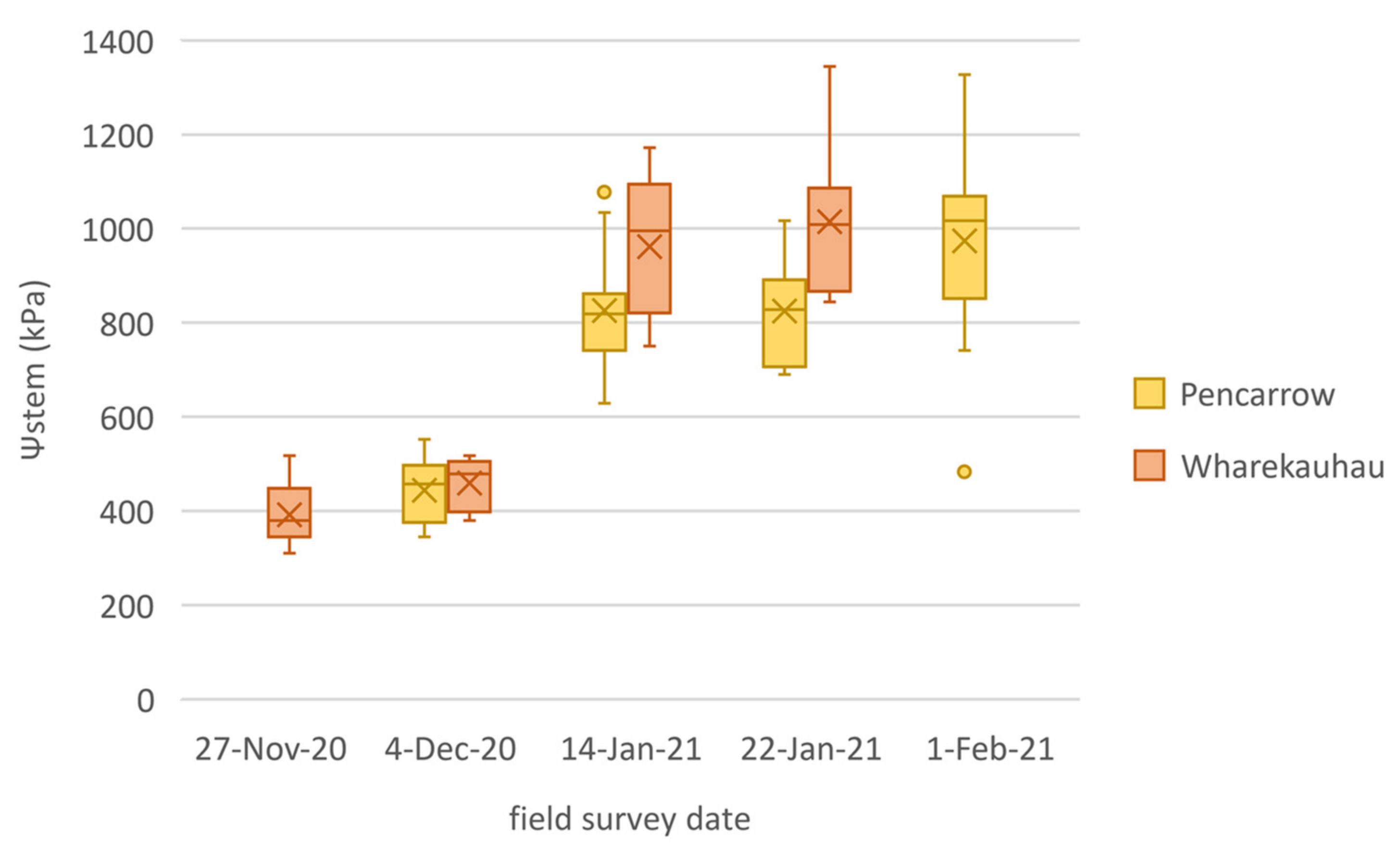
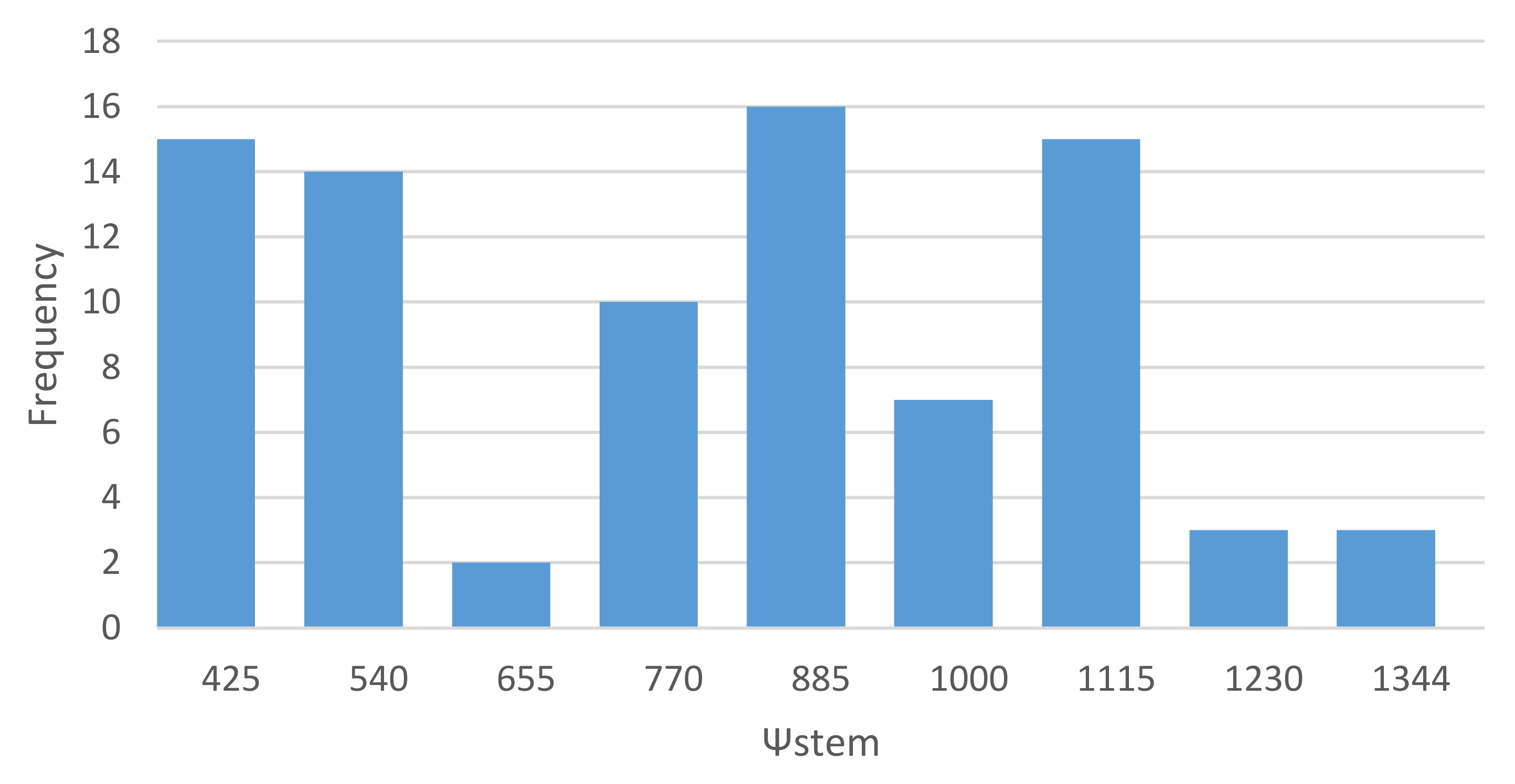
3.1. Variation in Vine Water Potential

Each vineyard was visited four times, from flowering through to veraison until netting the vines to protect from birds. This timeframe is the most critical in terms of the effects of GWS on berry quality before harvest. The underlying premise is that precise monitoring of GWS in this period is essential to produce grapes with premium quality. Figure 4 displays the variation of stem water potential (Ψstem) collected from different canopies over the five field survey days, and the distribution of the measurements on each date. There were no irrigation events during the field surveys, due to the adequate rainfall from late November to early December (Figure 4). As the recorded Ψstem is equal and opposite to the GWS, the effect of heavy rainfall was reflected by the high GWS observed at the initial survey. The subsequently increasing Ψstem values resulted from no irrigation plus little precipitation indicate the impact of water deficit gradually accumulating in the canopy as the survey proceeded from flowering to veraison. In terms of the full dataset, the collected leaf samples show a range of Ψstem values from 310 to 1344 kPa (

Table 6. Descriptive statistics of Ψstem (kPa) of all the observations (n = 85).

	Total Sample Size	Mean	Standard Deviation	Maximum	Minimum
Ψstem (kPa)	85	752	277	1344	310

). The frequency histogram in Figure 5 reveals the distribution of collected Ψstem values, and the class number was determined by the square root of the total sample number.

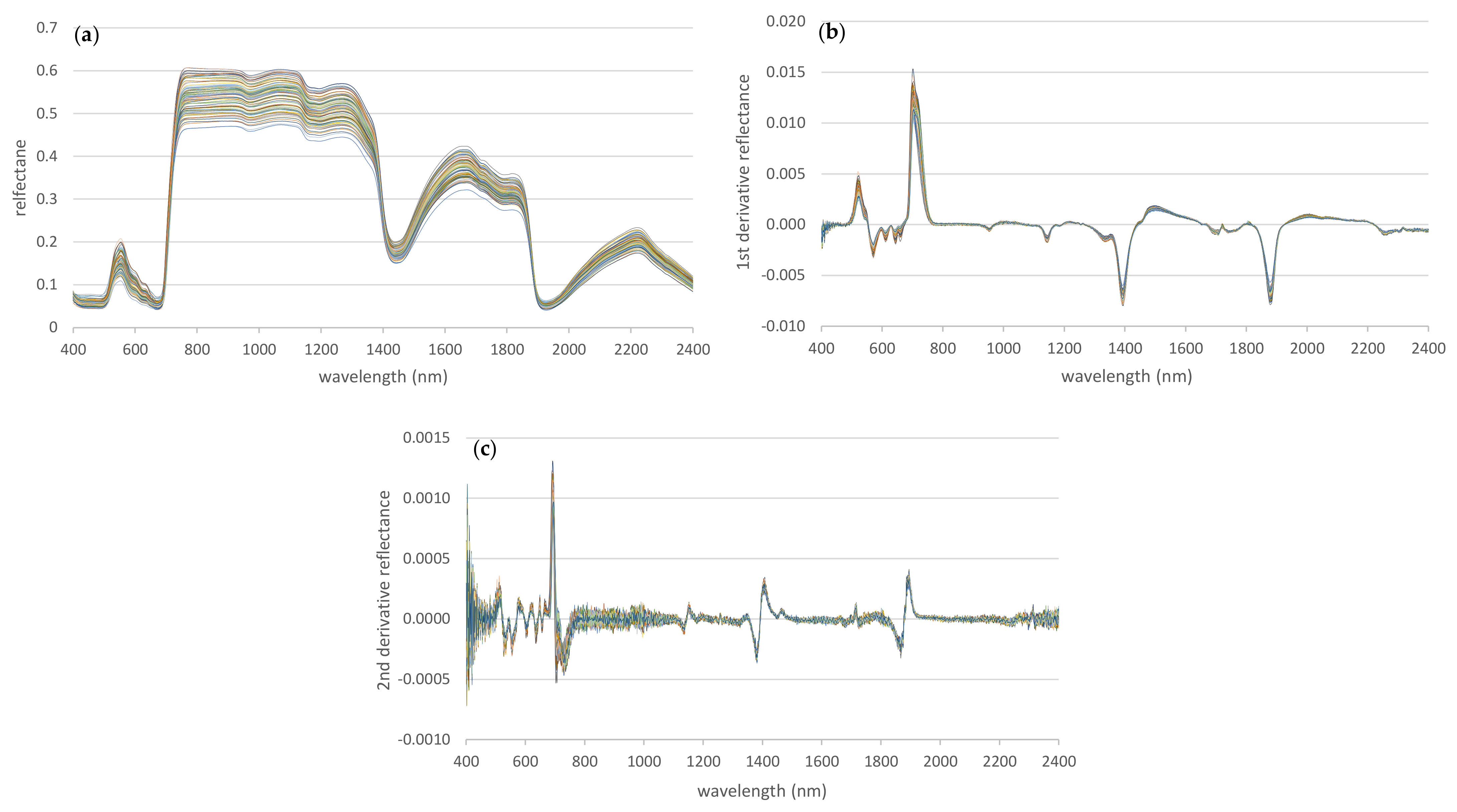
3.2. Variation in Hyperspectral Data

The raw reflectance in Figure 6a portrays typical reflectance patterns of healthy vegetation: Moderate reflectance at around 500–600 nm, due to the reflection of green light, strong reflectance at around 750–1300 nm, due to the healthy internal structure of leaves, two weak water absorption regions at around 970 and 1200 nm (NIR region), as well as two strong water absorption regions at around 1450 and 1900 nm (SWIR region). Reflectance differences at specific wavelengths over the full spectrum between samples will potentially enable us to estimate GWS for each observation. The spectral regions with evident dispersion of derivative curves may also be potentially linked to the vine’s hydration state, involving 400–800, 1300–1500, 1700, and 1900 nm for the first derivative reflectance, as well as 400–600, 700–1300, 1500–1900, and 2000–2400 nm for the second derivative reflectance (Figure 6b,c).

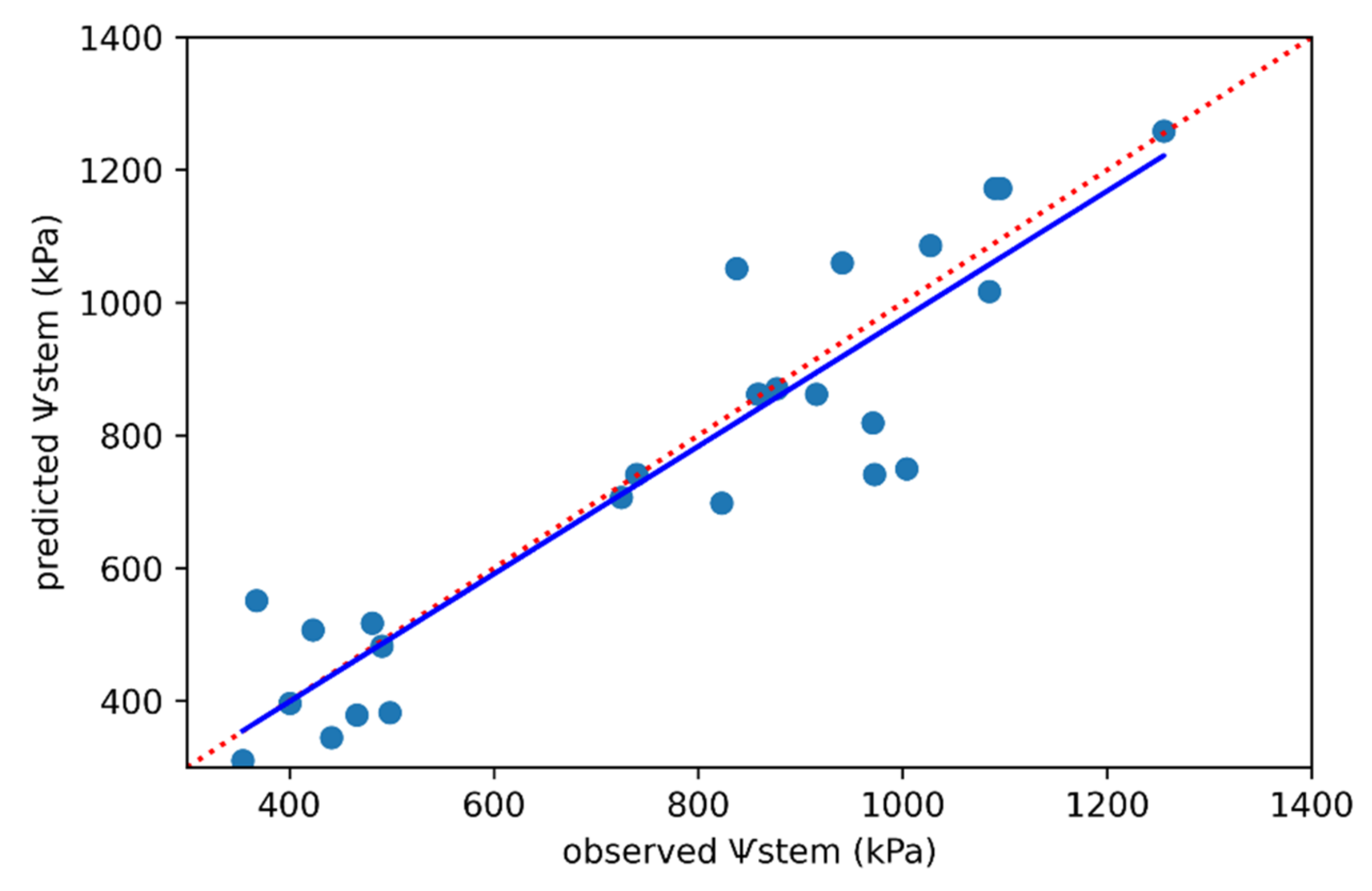
3.3. Modeling Performance

This study used combinations of six feature groups, two variable selection methods, an ensemble of selected variables, and three regression models to construct 38 modeling pipelines. Specifically, feature groups include raw reflectance, first derivative (1D) reflectance, second derivative (2D) reflectance, continuum removal (CR) variables, simple ratio indices (SI), and vegetation indices (VI). Variable selection methods include Spearman correlation and recursive feature elimination based on cross-validation (RFECV). Regression models include partial least squares regression (PLSR), random forest regression (RFR), and support vector regression (SVR). The modeling pipelines can be viewed as the pipelines without a variable selection component (i.e., pipelines with numbers 1–5, and 38 in Table 4), and with variable selection components (i.e., pipelines with numbers 6–37 in Table 4). The model evaluation metrics (i.e., R² and RMSE) were computed for modeling performance evaluation. For pipelines with numbers 6–37 in Table 4, only pipelines with the best performance on the test set are presented (

Table 7. Results of modeling performance on the test dataset.

	Metric	Partial Least Squares Regression	Random Forest Regression	Support Vector Regression
Feature group
Raw reflectance	R2	0.81	0.70	0.74
	RMSE	123	152	141
	Variable source	Full set	RFECV	RFECV
First derivative reflectance	R2	0.79	0.70	0.67
	RMSE	127	154	161
	Variable source	Full set	Spearman correlation	Spearman correlation
Second derivative reflectance	R2	0.65	0.71	0.68
	RMSE	166	150	158
	Variable source	Full set	Spearman correlation	Spearman correlation
Continuum removal variables	R2	0.70	0.66	0.63
	RMSE	152	162	170
	Variable source	Full set	Full set	Full set
Simple ratio indices	R2	0.85	0.67	0.78
	RMSE	110	160	131
	Variable source	Full set	RFECV	RFECV
N/A	R2	N/A	0.68	0.79
	RMSE	N/A	159	128
	Variable source	N/A	Ensemble of selected variables	Ensemble of selected variables

). The results implied by R² are equivalent to those implied by RMSE, as expected, since the best performance of modeling is based on the highest value of R² along with the lowest value of RMSE. Amongst all the modeling pipelines (i.e., pipelines with numbers 1–38 in Table 4), the best performance occurs when PLSR was trained with SI, resulting in the highest R² (0.85) and lowest RMSE (110 kPa). Its scatter plot, shown in Figure 7, presents the relationship between observed and predicted Ψstem. Either Spearman correlation or RFECV results improve the performance of RFR and SVR for all feature groups, except for CR variables. Amongst pipelines with numbers 6–37 in Table 4, SVR trained with the ensemble of selected variables results in the best performance. The modeling performance of Ψstem by VIs is poor, as none of the VI resulted in modeling with R² higher than 0.5. The best performance among all the models using VI as input variable was the one regressed with photochemical reflectance index (R² = 0.41; RMSE = 210 kPa).

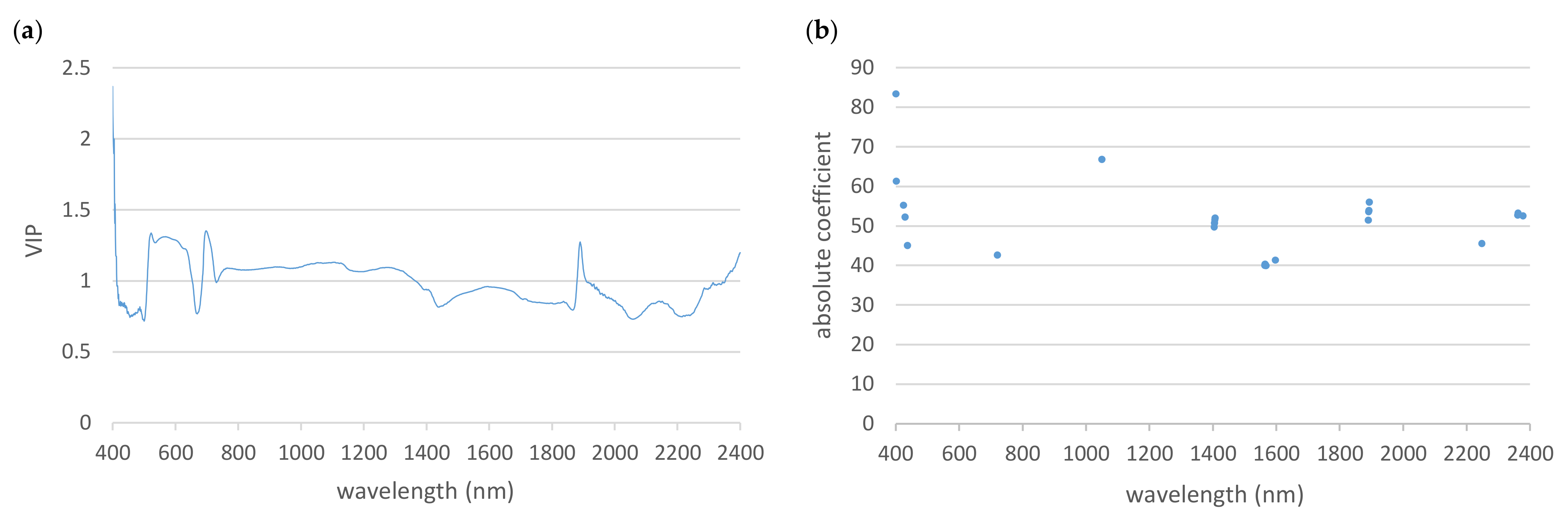
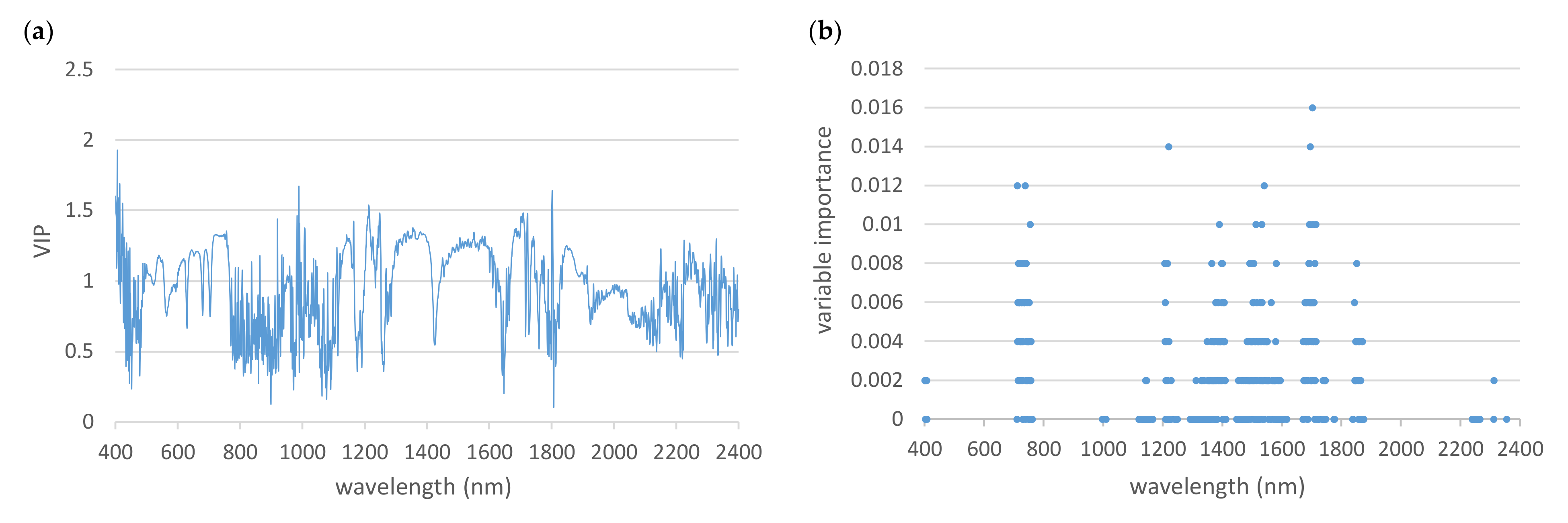
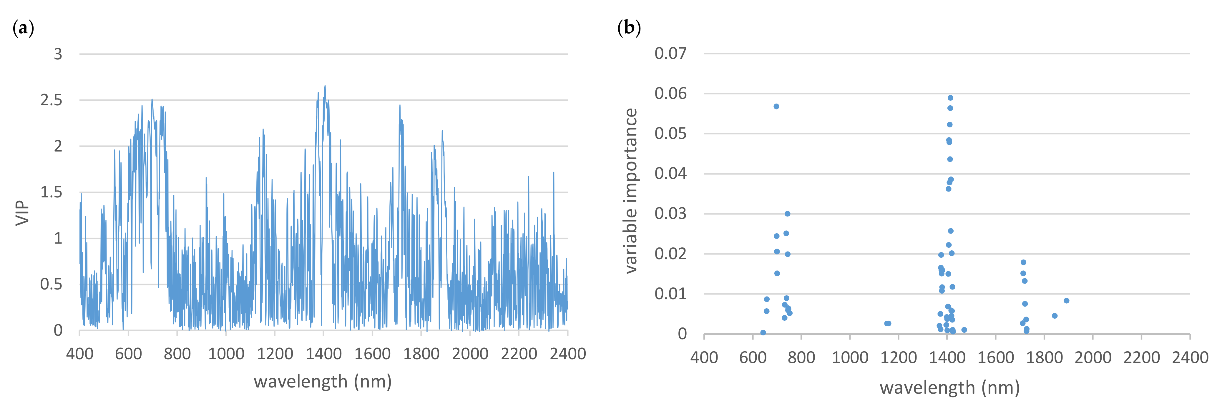
3.4. Selected Variables and Their Relative Importance

Figure 8, Figure 9, Figure 10, Figure 11 and Figure 12 present the variable importance for each of the five feature groups (raw reflectance, 1D, 2D, CR, and SI). PLSR uses variable importance in projection (VIP), RFR uses variable importance, and SVR uses coefficient to rank the significance for either the full set of variables, Spearman correlation-selected variables, or RFECV-selected variables. For pipelines with numbers 6–37 in Table 4, the variable importance was only calculated and presented for the variable subset used as inputs for the modeling pipelines with the best performance on the test set. That is, using SVR to compute variable importance for RFECV-selected variables from raw reflectance, using RFR trained to compute variable importance for Spearman correlation-selected variables from 1D reflectance, using RFR to compute variable importance for Spearman correlation-selected variables from 2D reflectance, using RFR to compute variable importance for the full set of variables of CR variables, and using SVR to compute variable importance for RFECV-selected variables from SI. This computation was based on the training set, and it can help elucidate significant regions and wavelengths relevant to Ψstem estimation.

3.4.1. Raw Reflectance

When using raw reflectance data, PLSR-based variable importance seems to be distributed evenly across 400–2400 nm. Although PLSR does not conduct variable selection, it calculates VIP for each wavelength to account for their significance in model construction. VIP values higher than one are generally considered significant. The VIP values for raw reflectance data fluctuate around one, with maxima occurring at around 400, 520–630, 700, 1890, and 2400 nm (Figure 8a). Variables selected by REFCV disperse at around 400–430, 720, 1049, 1400, 1565–1595, 1890, 2250, and 2370 nm (Figure 8b). Their variable importance computed by SVR indicates the region around 400–430 is the most important.

3.4.2. First Derivative

The VIP values derived from PLSR for each 1 D variable are more discrete compared to that for each raw reflectance variable, with the difference between the highest and lowest VIP values being larger (Figure 9a). With Spearman correlation, selected variables concentrate at around 400, 715–760, 800–1250, 1000–1870, and 2250–2350 nm (Figure 9b). The important regions computed by RFR are at around 740, 1220, and 1700 nm.

3.4.3. Second Derivative

The important 2 D variables computed based on VIP (Figure 10a) are even more discrete across the entire spectrum compared to those for 1 D reflectance. This implies that there are relatively few variables relevant to the variation of Ψstem values in this feature group. As the VIP values of several regions are close to zero, the significant spectral regions can be determined more clearly. Interestingly, the evident regions based on VIP values are quite similar, to those selected by the Spearman correlation. These regions are at around 650–750, 1155, 1370–1420, 1720, and 1870 nm (Figure 10b). It seems the regions at around 700 and 1410 were relatively more significant according to the variable importance computed by RFR.

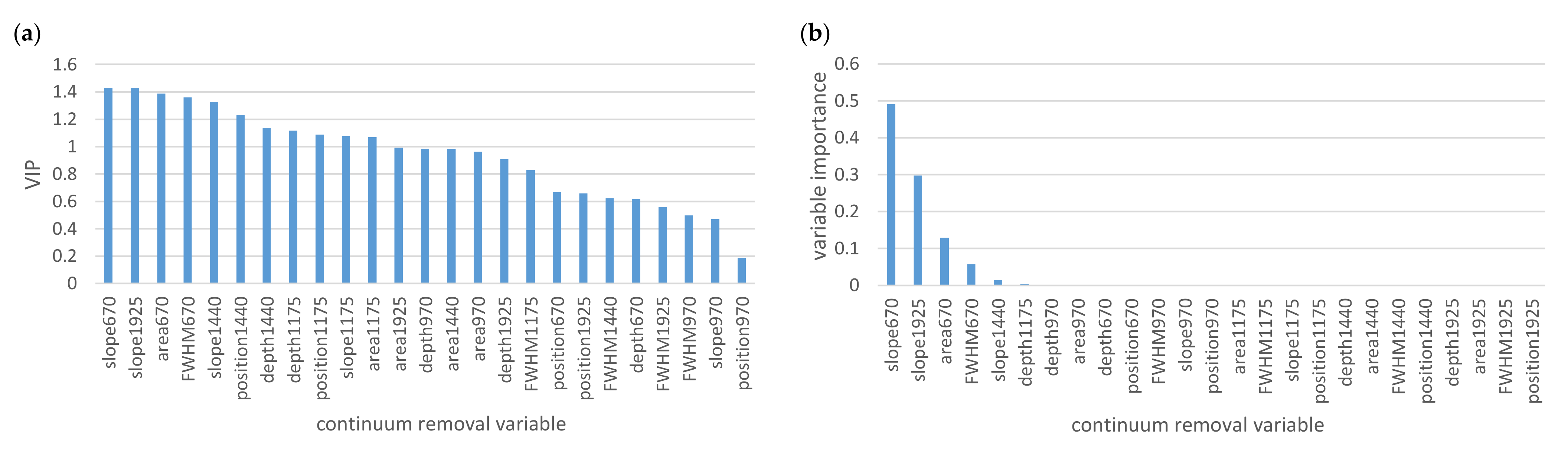
3.4.4. Continuum Removal Features

With CR variables, both RFR and SVR performed better when using the full set of variables. The top five important variables ranked by PLSR and RFR are the same (Figure 11), including continuum slope of the region centered at 670 nm, continuum slope of the region centered at 1925 nm, absorption area of the region centered at 670 nm, full width at half maximum of band depth (FWHM) of the region centered at 670 nm, and continuum slope of the region centered at 1440 nm.

3.4.5. Simple Ratio Indices

Most of the SI variables make similar contributions to the modeling according to the nondrastically different VIP values in the heatmap (Figure 12a). Several important regions can be identified based on the strip-like differences of color in the heatmap. They include the regions of 500–650, 700–730, 1400, 1700, 1900, and 2000–2400 nm. Some indices only play a significant role when formed by the reflectance of adjacent wavelengths, so there are evident differences of color in the heatmap close to the 1:1 line, involving 1050–1150, 1200–1300, and 1800 nm. RFECV-selected variables have similar significance based on absolute coefficient values computed by SVR (Figure 12b). Most of the selected indices are built based on the reflectance close to each other by wavelengths, and thus, the colored regions go along the 1:1 line. These regions mainly include 400–500, 750–1300, 1500–1850, 1900–2400 nm. Besides, some strip-like color bars indicate some selected indices are calculated by the ratios of reflectance between 400–600 and 700 nm, 1750–1850 and 1400 nm, as well as 2250–2350 and 1900 nm.

4. Discussion

This study attempts to establish a quantitative correlation between the spectral reflectance of vine canopy leaves in the VIS, NIR, and SWIR regions of the spectrum, and the Ψstem, which is used as a proxy for GWS. Since this relationship has been reported to be affected by numerous factors, including growing conditions, phenological stages [57], leaf homogeneity [56], cultivars [67], leaf age [68], and leaf position [69], the study trial was set up using the same cultivar with similar age and consistent sampling method throughout the field sampling to help minimize these factors. However, in situ heterogeneity of soil type and microclimate conditions will influence growth patterns and/or water stress levels within and between grapevines, so sampling was undertaken frequently over the critical period (late November to early February) to capture sufficient variability for analysis. Note that the number of data collected for this study is small (n = 85). In addition, these are commercial vineyards subjected to normal management practices, and one of the objectives of this study was to ensure that the collected data represented vine responses to these conditions as much as possible.

4.1. The Effects of Data Transformation on the Estimation of Grapevine Water Status

The models fitted using the SI outperformed those regressed with the other transformed data among pipelines with numbers 1–5 and among pipelines with numbers 6–37 in Table 4. When the input variables were augmented from 2001 reflectance values over 400–2400 nm to 2,001,000 ratio values, new information was produced, which largely increased the potential of correlation with Ψstem. It is observed 1D, 2D, CR transformations do not improve the modeling performance compared to models trained with raw reflectance data among pipelines. One possible reason for the poor performance of pipelines with CR preprocessing is that since the five selected spectral regions (560–750, 900–1060, 1080–1250, 1280–1660, and 1830–2210 nm) did not fully cover the entire study spectrum of 400–2400 nm, the rejected regions may have contained sufficient ‘diffuse’ information to affect modeling performance when correlating reflectance with Ψstem values. For this work, a plant probe with a stable incident angle and light intensity was used in contact with leaves to provide standardized survey conditions as described in Section 2.4. It minimized the influences, of illumination conditions, angle of the sun, and background interference on in situ spectral measurements. That is why original reflectance in this study can achieve high accuracy of Ψstem estimation, which supports the study of González-Fernández et al. [43].

4.2. Significantly Important Spectral Regions Derived from Variable Selection

Due to multicollinearity within the hyperspectral reflectance, the removal of noncontributing variables is problematic. However, it is important to remove less informative variables to help minimize modeling noise by these variables [70]. It is observed that Spearman correlation works better using 1D and 2D reflectance as input variables, and RFECV performs better using raw reflectance and SI as input variables. Raw reflectance and SI have much higher multicollinearity than 1D and 2D do according to the VIP values (Figure 8a, Figure 9a, Figure 10a, and Figure 12a). Since PLSR extracts the shared variance between predictor variables, the higher VIP values compared to predictor variables, the less correlation is between them. This observation is similar to the findings of Bhadra et al. [71]. However, they used Pearson correlation and RFR instead of Spearman correlation and RFECV to select variables. The full set of CR variables was selected, because this feature group is not highly dimensional, variable elimination may remove some relevant, but diffuse, variables, and thus, reduce modeling performance.

The important regions were those bounded by the spectral bands that were determined by the modeling pipelines with the highest estimation accuracy for each feature group. In the VIS spectrum, the important bands identified are 400–430 nm and 650–750 nm. The 400–430 nm band corresponds to the blue band representing strong absorption by chlorophyll-a, chlorophyll-b, and carotenoids (carotenes and xanthophylls). Variations in these compounds indicate cumulative effects of water stress, and are, thus, indirectly related to variation in GWS, and thus, Ψstem values [46]. The 650–750 nm corresponds to red and red edge bands and describes the concentrations [72] and ratios [20] of chlorophyll-a and -b, again indicating water stress status. The ranking of CR features indicates the absorption band at around 670 nm (slope, area, and full width at half maximum of band depth (FWHM)) is significant. These CR variables describe the shape of the absorption curve within this band. This has been observed in previous studies [73,74], which found that the position and shape of the absorption curve in the red edge band changed, due to water stress-induced changes of chlorophyll content in the vine leaves.

In the NIR spectrum, the important bands determined are 800–1250 nm. Within this band, there is a partial reflectance response to two weak water absorption bands at 970 and 1200 nm [75]. Variation of reflectance in this band can also be related to changes in internal leaf structure resulting from dehydration [76] and the decomposition of celluloses and proteins, due to water stress [13].

In the SWIR spectrum, the important bands identified are 1370–1420, 1500–1595, 1700–1720, 1850–1890, 2050–2370 nm. Reflectance responses in the SWIR spectrum are partially determined by dry leaf matter (i.e., lignin, cellulose, and protein), but mainly by two strong water absorption features centered at 1400 and 1940 nm [12]. Extra consideration should be given when using water absorption bands (1400 and 1940 nm) to estimate plant water status. The spectral reflectance acquired in this study was a contact measurement using a leaf clip and contact probe with artificial illumination. However, if GWS is estimated by airborne or space-borne data, the reflectance at 1400 and 1940 nm would become useless because the solar energy, as source illumination, is largely absorbed by atmospheric water vapor before reaching the surface of the earth. As dry leaf matter remains relatively constant under low water deficit regimes, water content is considered the dominant factor influencing the SWIR spectrum from 1300 to 2500 nm. However, as water stress increases and leaf water content declines, the effect of dry leaf matter on spectral reflectance becomes more apparent [14]. Disregarding the water absorption regions (1400 and 1940 nm), the remaining bands in the SWIR spectrum agree well with the findings of [10] (1520–1540 nm) and [77,78,79] (1650–1850 and 2000–2270 nm). For the CR feature group, bands (1280–1660, and 1830–2210 nm) were selected based on their continuum slope. This was calculated based on the ratio of the reflectance difference to the bandwidth. As the bandwidth was predetermined, the significance of continuum slope can be attributed to reflectance difference and suggests the potential to use reflectance differences as variables for estimating Ψstem.

The ensemble of selected variables in this study includes RFECV-selected variables from raw reflectance, Spearman correlation-selected variables from 1D reflectance, Spearman correlation-selected variables from 2D reflectance, full set of CR variables, and RFECV-selected variables from SI. This method, although not resulting in evident improvement of estimation accuracy, generated the highest R² of 0.79 and lowest RMSE of 128 on the test set among pipelines 6–37 in Table 4. This proves the benefit offered by ensemble technique beyond what can be achieved by a single combination of a data transformation technique and a variable selection method, which was proposed by Feilhauer et al. [36].

4.3. The Performance of Regression Models

Although previous studies have stated that the NIR-SWIR spectrum is more suitable for water status estimation [58,80], this paper suggests that statistically significant wavelengths correlated with Ψstem variation span several spectral regions over the entire spectrum, when different transformed datasets are used as inputs, in the modeling pipelines employed by this study. The poor performance of VI also implies the limitation of using the reflectance given at two to three wavelengths. This was in agreement with the study of Feilhauer et al. [36], which stated the spectral features related to biochemical indicators were dispersed across multiple bands, and thus, needed to be considered collectively. Therefore, the multivariate techniques that were utilized in this study attempted to make the best use of the entire hyperspectral spectrum instead of focusing on conventional indices derived from reflectance at two or three wavelengths. The advantage of this way has been demonstrated by Romero et al. [29]. PLSR, RFR, and SVR were regressed with either the entire spectrum or a subset of this spectrum. Despite the high dimensionality and multicollinearity inherent in hyperspectral data, PLSR can reduce this complexity down to a few independent variables and attained the best accuracy for Ψstem estimation. One explanation is that PLSR can effectively integrate the shared variance of both directly and indirectly relevant bands, as explained in Section 4.2. This capability has also been observed by several studies using the same technique to estimate crop water status from hyperspectral data [30,80,81,82]. Since PLSR simulates a linear relationship, this suggests that there is a linear relationship between the extracted information from important bands and Ψstem values for all the feature groups except 2D reflectance. One possible explanation is that its relationship with Ψstem may not be best described by a linear model, such as PLSR. Since RFR and SVR are able, to simulate nonlinearity, this may be the reason why these two models can outperform PLSR when using 2D reflectance as the input dataset. Reduced variable size resulting from variable selection improves the performance of RFR and SVR for most of the feature groups except for CR variables. RFR and SVR were reported to show robustness on high-dimensional data [26,31,66]. However, this study demonstrates the advantages of variable selection in terms of increasing model performance by RFR and SVR. This may be attributed to the decreased collinearity in the reduced input data. SVR has been found (in other studies [32]) to suffer from multicollinearity when fitted using the full-spectrum datasets, with improved performance when the most informative bands were used as input data instead.

5. Conclusions

This study investigated the relationship between stem water potential (Ψstem) and leaf-scale hyperspectral reflectance (400–2400 nm) collected between late November 2020 and early February 2021 from two New Zealand vineyards using 38 modeling pipelines. These pipelines show that partial least squares regression trained with simple ratio indices based on the entire spectrum provided the best Ψstem predictions (R² = 0.85; RMSE = 110 kPa), significantly outperforming the linear regression using classical vegetation index as an input variable. Additional results reveal the benefit of increasing accuracy at Ψstem prediction using an ensemble of selected variables composed of multicombination of transformed data and variable selection methods. The above-mentioned outcomes can be used to tailor an automatic data processing and modeling pipeline to estimate Ψstem. Accordingly, if sufficient hyperspectral measurements are undertaken, this will provide a means of delivering a rapid and nondestructive estimation of Ψstem, and thus, grapevine water status. Information on individual grapevine water status should enable vineyards to tailor irrigation on a per vine basis rather than a per block status, which is the general practice at present. This would enable better control of the desirable traits in the grape berries, that are affected by water content. This would improve wine quality, and therefore, the price achieved. Due to the limited data size obtained in this study, future studies can potentially focus on validating these pipelines using more samples collected from different growing stages and years. Extra consideration should be taken when using airborne or space-borne imaging for estimation, because of water absorption bands. However, more research is required to be carried out, and this study has proved a concept of estimating grapevine water status using a ground-based hyperspectral spectroradiometer.

References

1. Chaves, M.M.; Zarrouk, O.; Francisco, R.; Costa, J.M.; Santos, T.; Regalado, A.P.; Rodrigues, M.L.; Lopes, C.M. Grapevine under deficit irrigation: Hints from physiological and molecular data. Ann. Bot. 2010, 105, 661–676. [Google Scholar] [CrossRef] [Green Version]
2. Ojeda, H.; Andary, C.; Kraeva, E.; Carbonneau, A.; Deloire, A. Influence of pre-and postveraison water deficit on synthesis and concentration of skin phenolic compounds during berry growth of Vitis vinifera cv. Shiraz. Am. J. Enol. Vitic. 2002, 53, 261–267. [Google Scholar]
3. Van Leeuwen, C.; Trégoat, O.; Choné, X.; Bois, B.; Pernet, D.; Gaudillère, J.-P. Vine water status is a key factor in grape ripening and vintage quality for red Bordeaux wine. How can it be assessed for vineyard management purposes? OENO One 2009, 43, 121–134. [Google Scholar] [CrossRef]
4. Acevedo-Opazo, C.; Tisseyre, B.; Guillaume, S.; Ojeda, H. The potential of high spatial resolution information to define within-vineyard zones related to vine water status. Precis. Agric. 2008, 9, 285–302. [Google Scholar] [CrossRef] [Green Version]
5. Ojeda, H.; Carrillo, N.; Deis, L.; Tisseyre, B.; Heywang, M.; Carbonneau, A. Precision viticulture and water status II: Quantitative and qualitative performance of different within field zones, defined from water potential mapping. In Proceedings of the XIV International GESCO Viticulture Congress, Groupe d’Etude des Systemes de COnduite de la vigne (GESCO), Geisenheim, Germany, 23–27 August 2005; pp. 741–748. [Google Scholar]
6. Rienth, M.; Scholasch, T. State-of-the-art of tools and methods to assess vine water status. OENO One 2019, 53, 619–637. [Google Scholar] [CrossRef]
7. Lavoie-Lamoureux, A.; Sacco, D.; Risse, P.A.; Lovisolo, C. Factors influencing stomatal conductance in response to water availability in grapevine: A meta-analysis. Physiol. Plant 2017, 159, 468–482. [Google Scholar] [CrossRef]
8. Oumar, Z.; Mutanga, O. Predicting plant water content in Eucalyptus grandis forest stands in KwaZulu-Natal, South Africa using field spectra resampled to the Sumbandila Satellite Sensor. Int. J. Appl. Earth Obs. Geoinf. 2010, 12, 158–164. [Google Scholar] [CrossRef]
9. Elsayed, S.; Mistele, B.; Schmidhalter, U. Can changes in leaf water potential be assessed spectrally? Funct. Plant Biol. 2011, 38, 523–533. [Google Scholar] [CrossRef] [PubMed]
10. Sims, D.A.; Gamon, J.A. Estimation of vegetation water content and photosynthetic tissue area from spectral reflectance: A comparison of indices based on liquid water and chlorophyll absorption features. Remote Sens. Environ. 2003, 84, 526–537. [Google Scholar] [CrossRef]
11. Gausman, H.W. Leaf reflectance of near infrared. Photogramm. Eng. 1974, 40, 183–191. [Google Scholar]
12. Curran, P.J. Remote sensing of foliar chemistry. Remote Sens. Environ. 1989, 30, 271–278. [Google Scholar] [CrossRef]
13. Yin, W.; Zhang, C.; Zhu, H.; Zhao, Y.; He, Y. Application of near-infrared hyperspectral imaging to discriminate different geographical origins of Chinese wolfberries. PLoS ONE 2017, 12, e0180534. [Google Scholar] [CrossRef] [PubMed] [Green Version]
14. Gao, B.-C.; Goetz, A.F. Extraction of dry leaf spectral features from reflectance spectra of green vegetation. Remote Sens. Environ. 1994, 47, 369–374. [Google Scholar] [CrossRef]
15. Rodríguez-Pérez, J.R.; Ordóñez, C.; González-Fernández, A.B.; Sanz-Ablanedo, E.; Valenciano, J.B.; Marcelo, V. Leaf water content estimation by functional linear regression of field spectroscopy data. Biosyst. Eng. 2018, 165, 36–46. [Google Scholar] [CrossRef]
16. Maimaitiyiming, M.; Ghulam, A.; Bozzolo, A.; Wilkins, J.L.; Kwasniewski, M.T. Early Detection of Plant Physiological Responses to Different Levels of Water Stress Using Reflectance Spectroscopy. Remote Sens. 2017, 9, 745. [Google Scholar] [CrossRef] [Green Version]
17. Pôças, I.; Rodrigues, A.; Gonçalves, S.; Costa, P.M.; Gonçalves, I.; Pereira, L.S.; Cunha, M. Predicting Grapevine Water Status Based on Hyperspectral Reflectance Vegetation Indices. Remote Sens. 2015, 7, 16460–16479. [Google Scholar] [CrossRef] [Green Version]
18. Rodríguez-Pérez, J.R.; Riano, D.; Carlisle, E.; Ustin, S.; Smart, D.R. Evaluation of hyperspectral reflectance indexes to detect grapevine water status in vineyards. Am. J. Enol. Vitic. 2007, 58, 302–317. [Google Scholar]
19. Loggenberg, K.; Strever, A.; Greyling, B.; Poona, N. Modelling Water Stress in a Shiraz Vineyard Using Hyperspectral Imaging and Machine Learning. Remote Sens. 2018, 10, 202. [Google Scholar] [CrossRef] [Green Version]
20. Zovko, M.; Žibrat, U.; Knapič, M.; Kovačić, M.B.; Romić, D. Hyperspectral remote sensing of grapevine drought stress. Precis. Agric. 2019, 20, 335–347. [Google Scholar] [CrossRef]
21. Fortin, M.; Dale, M.R.T. Spatial Analysis: A Guide for Ecologists; Cambridge University Press: Cambridge, UK, 2005. [Google Scholar]
22. Li, X.; Zhang, Y.; Bao, Y.; Luo, J.; Jin, X.; Xu, X.; Song, X.; Yang, G. Exploring the Best Hyperspectral Features for LAI Estimation Using Partial Least Squares Regression. Remote Sens. 2014, 6, 6221–6241. [Google Scholar] [CrossRef] [Green Version]
23. Vasques, G.; Grunwald, S.; Sickman, J. Comparison of multivariate methods for inferential modeling of soil carbon using visible/near-infrared spectra. Geoderma 2008, 146, 14–25. [Google Scholar] [CrossRef]
24. Kokaly, R.F.; Clark, R.N. Spectroscopic determination of leaf biochemistry using band-depth analysis of absorption features and stepwise multiple linear regression. Remote Sens. Environ. 1999, 67, 267–287. [Google Scholar] [CrossRef]
25. Zarco-Tejada, P.J.; Pushnik, J.C.; Dobrowski, S.; Ustin, S. Steady-state chlorophyll a fluorescence detection from canopy derivative reflectance and double-peak red-edge effects. Remote Sens. Environ. 2003, 84, 283–294. [Google Scholar] [CrossRef]
26. Doktor, D.; Lausch, A.; Spengler, D.; Thurner, M. Extraction of Plant Physiological Status from Hyperspectral Signatures Using Machine Learning Methods. Remote Sens. 2014, 6, 12247–12274. [Google Scholar] [CrossRef] [Green Version]
27. Chandrashekar, G.; Sahin, F. A survey on feature selection methods. Comput. Electr. Eng. 2014, 40, 16–28. [Google Scholar] [CrossRef]
28. James, G.; Witten, D.; Hastie, T.; Tibshirani, R. An Introduction to Statistical Learning; Springer: New York, NY, USA, 2013; Volume 112. [Google Scholar]
29. Romero, M.; Luo, Y.; Su, B.; Fuentes, S. Vineyard water status estimation using multispectral imagery from an UAV platform and machine learning algorithms for irrigation scheduling management. Comput. Electron. Agric. 2018, 147, 109–117. [Google Scholar] [CrossRef]
30. Das, B.; Sahoo, R.N.; Pargal, S.; Krishna, G.; Verma, R.; Viswanathan, C.; Sehgal, V.K.; Gupta, V.K. Evaluation of different water absorption bands, indices and multivariate models for water-deficit stress monitoring in rice using visible-near infrared spectroscopy. Spectrochim. Acta Part A Mol. Biomol. Spectrosc. 2021, 247, 119104. [Google Scholar] [CrossRef]
31. Wang, L.; Zhou, X.; Zhu, X.; Dong, Z.; Guo, W. Estimation of biomass in wheat using random forest regression algorithm and remote sensing data. Crop. J. 2016, 4, 212–219. [Google Scholar] [CrossRef] [Green Version]
32. Axelsson, C.; Skidmore, A.K.; Schlerf, M.; Fauzi, A.; Verhoef, W. Hyperspectral analysis of mangrove foliar chemistry using PLSR and support vector regression. Int. J. Remote Sens. 2012, 34, 1724–1743. [Google Scholar] [CrossRef]
33. Du, P.; Xia, J.; Chanussot, J.; He, X. Hyperspectral remote sensing image classification based on the integration of support vector machine and random forest. In Proceedings of the 2012 IEEE International Geoscience and Remote Sensing Symposium, Munich, Germany, 22–27 July 2012. [Google Scholar]
34. Engler, R.; Waser, L.T.; Zimmermann, N.E.; Schaub, M.; Berdos, S.; Ginzler, C.; Psomas, A. Combining ensemble modeling and remote sensing for mapping individual tree species at high spatial resolution. For. Ecol. Manag. 2013, 310, 64–73. [Google Scholar] [CrossRef]
35. Xu, M.; Liu, H.; Beck, R.; Lekki, J.; Yang, B.; Shu, S.; Kang, E.; Anderson, R.; Johansen, R.; Emery, E.; et al. A spectral space partition guided ensemble method for retrieving chlorophyll-a concentration in inland waters from Sentinel-2A satellite imagery. J. Great Lakes Res. 2019, 45, 454–465. [Google Scholar] [CrossRef]
36. Feilhauer, H.; Asner, G.P.; Martin, R.E. Multi-method ensemble selection of spectral bands related to leaf biochemistry. Remote Sens. Environ. 2015, 164, 57–65. [Google Scholar] [CrossRef]
37. Seijo-Pardo, B.; Bolón-Canedo, V.; Alonso-Betanzos, A. On developing an automatic threshold applied to feature selection ensembles. Inf. Fusion 2019, 45, 227–245. [Google Scholar] [CrossRef]
38. Pôças, I.; Gonçalves, J.; Costa, P.M.; Gonçalves, I.; Pereira, L.S.; Cunha, M. Hyperspectral-based predictive modelling of grapevine water status in the Portuguese Douro wine region. Int. J. Appl. Earth Obs. Geoinformation 2017, 58, 177–190. [Google Scholar] [CrossRef]
39. Tosin, R.; Pôças, I.; Gonçalves, J.; Cunha, M. Estimation of grapevine predawn leaf water potential based on hyperspectral reflectance data in Douro wine region. Vitis 2020, 59, 9–18. [Google Scholar]
40. Krishna, G.; Sahoo, R.N.; Singh, P.; Bajpai, V.; Patra, H.; Kumar, S.; Dandapani, R.; Gupta, V.K.; Viswanathan, C.; Ahmad, T.; et al. Comparison of various modelling approaches for water deficit stress monitoring in rice crop through hyperspectral remote sensing. Agric. Water Manag. 2019, 213, 231–244. [Google Scholar] [CrossRef]
41. Choné, X.; Van Leeuwen, C.; Dubourdieu, D.; Gaudillère, J.P. Stem Water Potential is a Sensitive Indicator of Grapevine Water Status. Ann. Bot. 2001, 87, 477–483. [Google Scholar] [CrossRef] [Green Version]
42. Demetriades-Shah, T.H.; Steven, M.D.; Clark, J.A. High resolution derivative spectra in remote sensing. Remote Sens. Environ. 1990, 33, 55–64. [Google Scholar] [CrossRef]
43. González-Fernández, A.B.; Sanz-Ablanedo, E.; Gabella, V.M.; García-Fernández, M.; Rodríguez-Pérez, J.R. Field Spectroscopy: A Non-Destructive Technique for Estimating Water Status in Vineyards. Agron 2019, 9, 427. [Google Scholar] [CrossRef] [Green Version]
44. Cao, Z.; Wang, Q.; Zheng, C. Best hyperspectral indices for tracing leaf water status as determined from leaf dehydration experiments. Ecol. Indic. 2015, 54, 96–107. [Google Scholar] [CrossRef]
45. González-Fernández, A.B.; Rodriguez-Perez, J.R.; Marabel, M.; Taboada, M.F. Álvarez Spectroscopic estimation of leaf water content in commercial vineyards using continuum removal and partial least squares regression. Sci. Hortic. 2015, 188, 15–22. [Google Scholar] [CrossRef]
46. Zarco-Tejada, P.J.; Gonzalez-Dugo, V.; Williams, L.; Suárez, L.; Jimenez-Berni, J.A.; Goldhamer, D.; Fereres, E. A PRI-based water stress index combining structural and chlorophyll effects: Assessment using diurnal narrow-band airborne imagery and the CWSI thermal index. Remote Sens. Environ. 2013, 138, 38–50. [Google Scholar] [CrossRef]
47. Le Maire, G.; François, C.; Soudani, K.; Berveiller, D.; Pontailler, J.-Y.; Bréda, N.; Genet, H.; Davi, H.; Dufrêne, E. Calibration and validation of hyperspectral indices for the estimation of broadleaved forest leaf chlorophyll content, leaf mass per area, leaf area index and leaf canopy biomass. Remote Sens. Environ. 2008, 112, 3846–3864. [Google Scholar] [CrossRef]
48. Jordan, C.F. Derivation of Leaf-Area Index from Quality of Light on the Forest Floor. Ecology 1969, 50, 663–666. [Google Scholar] [CrossRef]
49. Hunt, E.R., Jr.; Rock, B.N. Detection of changes in leaf water content using near-and middle-infrared reflectances. Remote Sens. Environ. 1989, 30, 43–54. [Google Scholar]
50. Gamon, J.A.; Peñuelas, J.; Field, C.B. A narrow-waveband spectral index that tracks diurnal changes in photosynthetic efficiency. Remote Sens. Environ. 1992, 41, 35–44. [Google Scholar] [CrossRef]
51. Peñuelas, J.; Gamon, J.; Griffin, K.L.; Field, C.B. Assessing community type, plant biomass, pigment composition, and photosynthetic efficiency of aquatic vegetation from spectral reflectance. Remote Sens. Environ. 1993, 46, 110–118. [Google Scholar] [CrossRef]
52. Gao, B.-C. NDWI—A normalized difference water index for remote sensing of vegetation liquid water from space. Remote Sens. Environ. 1996, 58, 257–266. [Google Scholar] [CrossRef]
53. Zarco-Tejada, P.J.; Miller, J.; Noland, T.; Mohammed, G.; Sampson, P. Scaling-up and model inversion methods with narrowband optical indices for chlorophyll content estimation in closed forest canopies with hyperspectral data. IEEE Trans. Geosci. Remote Sens. 2001, 39, 1491–1507. [Google Scholar] [CrossRef] [Green Version]
54. Strachan, I.B.; Pattey, E.; Boisvert, J.B. Impact of nitrogen and environmental conditions on corn as detected by hyperspectral reflectance. Remote Sens. Environ. 2002, 80, 213–224. [Google Scholar] [CrossRef]
55. Eitel, J.U.; Gessler, P.E.; Smith, A.; Robberecht, R. Suitability of existing and novel spectral indices to remotely detect water stress in Populus spp. For. Ecol. Manag. 2006, 229, 170–182. [Google Scholar] [CrossRef]
56. Seelig, H.-D.; Adams, W.W.; Hoehn, A.; Stodieck, L.S.; Klaus, D.M.; Emery, W.J. Extraneous variables and their influence on reflectance-based measurements of leaf water content. Irrig. Sci. 2008, 26, 407–414. [Google Scholar] [CrossRef]
57. Wang, Q.; Li, P. Identification of robust hyperspectral indices on forest leaf water content using PROSPECT simulated dataset and field reflectance measurements. Hydrol. Process. 2011, 26, 1230–1241. [Google Scholar] [CrossRef]
58. Rapaport, T.; Hochberg, U.; Shoshany, M.; Karnieli, A.; Rachmilevitch, S. Combining leaf physiology, hyperspectral imaging and partial least squares-regression (PLS-R) for grapevine water status assessment. ISPRS J. Photogramm. Remote Sens. 2015, 109, 88–97. [Google Scholar] [CrossRef]
59. Guyon, I.; Elisseeff, A. An introduction to variable and feature selection. J. Mach. Learn. Res. 2003, 3, 1157–1182. [Google Scholar]
60. Gregorutti, B.; Michel, B.; Saint-Pierre, P. Correlation and variable importance in random forests. Stat. Comput. 2017, 27, 659–678. [Google Scholar] [CrossRef] [Green Version]
61. Martens, H.; Naes, T. Multivariate Calibration; John Wiley & Sons: Hoboken, NJ, USA, 1992. [Google Scholar]
62. Eriksson, L.; Byrne, T.; Johansson, E.; Trygg, J.; Vikstrom, C. Multi-and Megavariate Data Analysis Basic Principles and Applications; Umetrics Academy: Umeå, Sweden, 2013; Volume 1. [Google Scholar]
63. Breiman, L. Random forests. Mach. Learn. 2001, 45, 5–32. [Google Scholar] [CrossRef] [Green Version]
64. Smola, A.J.; Schölkopf, B. A tutorial on support vector regression. Stat. Comput. 2004, 14, 199–222. [Google Scholar] [CrossRef] [Green Version]
65. Hua, J.; Xiong, Z.; Lowey, J.; Suh, E.; Dougherty, E.R. Optimal number of features as a function of sample size for various classification rules. Bioinformatics 2004, 21, 1509–1515. [Google Scholar] [CrossRef] [Green Version]
66. Stamenkovic, J.; Tuia, D.; de Morsier, F.; Borgeaud, M.; Thiran, J.P. Estimation of soil moisture from airborne hyperspectral imagery with support vector regression. In Proceedings of the 2013 5th Workshop on Hyperspectral Image and Signal Processing: Evolution in Remote Sensing (WHISPERS), Gainesville, FL, USA, 26–28 June 2013. [Google Scholar]
67. Gutiérrez-Gamboa, G.; Pérez-Donoso, A.G.; Pou-Mir, A.; Acevedo-Opazo, C.; Valdés-Gómez, H. Hydric behaviour and gas exchange in different grapevine varieties (Vitis vinifera L.) from the Maule Valley (Chile). S. Afr. J. Enol. Vitic. 2019, 40, 1. [Google Scholar] [CrossRef]
68. Guyot, G. Optical properties of vegetation canopies. Appl. Remote Sens. Agric. 1990, 19–43. [Google Scholar] [CrossRef]
69. Turner, N.C. Measurement of plant water status by the pressure chamber technique. Irrig. Sci. 1988, 9, 289–308. [Google Scholar] [CrossRef]
70. Xiaobo, Z.; Jiewen, Z.; Povey, M.; Holmes, M.; Hanpin, M. Variables selection methods in near-infrared spectroscopy. Anal. Chim. Acta 2010, 667, 14–32. [Google Scholar] [CrossRef]
71. Bhadra, S.; Sagan, V.; Maimaitijiang, M.; Maimaitiyiming, M.; Newcomb, M.; Shakoor, N.; Mockler, T. Quantifying Leaf Chlorophyll Concentration of Sorghum from Hyperspectral Data Using Derivative Calculus and Machine Learning. Remote Sens. 2020, 12, 2082. [Google Scholar] [CrossRef]
72. Ballester, C.; Zarco-Tejada, P.J.; Nicolás, E.; Alarcon, J.J.; Fereres, E.; Intrigliolo, D.S.; Gonzalez-Dugo, V. Evaluating the performance of xanthophyll, chlorophyll and structure-sensitive spectral indices to detect water stress in five fruit tree species. Precis. Agric. 2018, 19, 178–193. [Google Scholar] [CrossRef]
73. Blackburn, G.A. Wavelet decomposition of hyperspectral data: A novel approach to quantifying pigment concentrations in vegetation. Int. J. Remote Sens. 2007, 28, 2831–2855. [Google Scholar] [CrossRef]
74. Campbell, P.K.E.; Middleton, E.M.; McMurtrey, J.E.; Corp, L.A.; Chappelle, E.W. Assessment of Vegetation Stress Using Reflectance or Fluorescence Measurements. J. Environ. Qual. 2007, 36, 832–845. [Google Scholar] [CrossRef]
75. Woolley, J.T. Reflectance and transmittance of light by leaves. Plant Physiol. 1971, 47, 656–662. [Google Scholar] [CrossRef] [Green Version]
76. Jacquemoud, S.; Baret, F. PROSPECT: A model of leaf optical properties spectra. Remote Sens. Environ. 1990, 34, 75–91. [Google Scholar] [CrossRef]
77. Cheng, T.; Rivard, B.; Sanchez-Azofeifa, A. Spectroscopic determination of leaf water content using continuous wavelet analysis. Remote Sens. Environ. 2011, 115, 659–670. [Google Scholar] [CrossRef]
78. Tian, Q.; Tong, Q.; Pu, R.; Guo, X.; Zhao, C. Spectroscopic determination of wheat water status using 1650–1850 nm spectral absorption features. Int. J. Remote Sens. 2001, 22, 2329–2338. [Google Scholar] [CrossRef]
79. Thulin, S.; Hill, M.; Held, A.; Jones, S.; Woodgate, P. Predicting Levels of Crude Protein, Digestibility, Lignin and Cellulose in Temperate Pastures Using Hyperspectral Image Data. Am. J. Plant Sci. 2014, 5, 997–1019. [Google Scholar] [CrossRef] [Green Version]
80. Rallo, G.; Minacapilli, M.; Ciraolo, G.; Provenzano, G. Detecting crop water status in mature olive groves using vegetation spectral measurements. Biosyst. Eng. 2014, 128, 52–68. [Google Scholar] [CrossRef]
81. Cassel, C.; Hackl, P.; Westlund, A.H. Robustness of partial least-squares method for estimating latent variable quality structures. J. Appl. Stat. 1999, 26, 435–446. [Google Scholar] [CrossRef]
82. Colombo, R.; Meroni, M.; Marchesi, A.; Busetto, L.; Rossini, M.; Giardino, C.; Panigada, C. Estimation of leaf and canopy water content in poplar plantations by means of hyperspectral indices and inverse modeling. Remote Sens. Environ. 2008, 112, 1820–1834. [Google Scholar] [CrossRef]
Figure 1. Location of study vineyards.
Remotesensing 13 03198 g001
Figure 2. Average daily temperature (red line) and accumulated daily rainfall (blue bars) recorded by the weather station at Palliser Estate between 27 November 2019 and 1 February 2021.
Remotesensing 13 03198 g002
Figure 3. Surveyed canopies (blue points) in Wharekauhau (a) and Pencarrow (b) vineyards.
Remotesensing 13 03198 g003
Figure 4. Boxplot of stem water potential (Ψstem) values for the full set of samples collected at Wharekauhau (n = 35) and Pencarrow (n = 50) vineyard.
Remotesensing 13 03198 g004
Figure 5. Distribution of Ψstem (kPa) for all the samples (n = 85). The dataset is not normally distributed.
Remotesensing 13 03198 g005
Figure 6. Raw hyperspectral signatures (a) and their first (b) and second (c) derivatives for all samples (n = 85).
Remotesensing 13 03198 g006
Figure 7. Scatter plots between predicted and observed Ψstem (kPa) simulated on the test set (n = 26) using the top-performing models—partial least squares regression (PLSR) trained with simple ratio indices (SI). The blue line is the regression line, and the red dotted line is the 1:1 line.
Remotesensing 13 03198 g007
Figure 8. Variable importance for raw reflectance data computed by PLSR (a), and support vector regression (SVR) based on variables selected by cross-validated recursive feature elimination (RFECV) (b).
Remotesensing 13 03198 g008
Figure 9. Variable importance for first derivative reflectance computed by PLSR (a), and random forest regression (RFR) based on Spearman correlation-selected variables (b).
Remotesensing 13 03198 g009
Figure 10. Variable importance for second derivative reflectance computed by PLSR (a), and RFR based on Spearman correlation-selected variables (b).
Remotesensing 13 03198 g010
Figure 11. Variable importance for continuum removal variables computed by PLSR (a), and RFR (b).
Remotesensing 13 03198 g011
Figure 12. Variable importance for simple ratio indices computed by PLSR (a) and SVR based on RFECV-selected variables (b).
Remotesensing 13 03198 g012