Abstract
The recent trend of automated machine learning (AutoML) has been driving further significant technological innovation in the application of artificial intelligence from its automated algorithm selection and hyperparameter optimization of the deployable pipeline model for unraveling substance problems. However, a current knowledge gap lies in the integration of AutoML technology and unmanned aircraft systems (UAS) within image-based data classification tasks. Therefore, we employed a state-of-the-art (SOTA) and completely open-source AutoML framework, Auto-sklearn, which was constructed based on one of the most widely used ML systems: Scikit-learn. It was combined with two novel AutoML visualization tools to focus particularly on the recognition and adoption of UAS-derived multispectral vegetation indices (VI) data across a diverse range of agricultural management practices (AMP). These include soil tillage methods (STM), cultivation methods (CM), and manure application (MA), and are under the four-crop combination fields (i.e., red clover-grass mixture, spring wheat, pea-oat mixture, and spring barley). Furthermore, they have currently not been efficiently examined and accessible parameters in UAS applications are absent for them. We conducted the comparison of AutoML performance using three other common machine learning classifiers, namely Random Forest (RF), support vector machine (SVM), and artificial neural network (ANN). The results showed AutoML achieved the highest overall classification accuracy numbers after 1200 s of calculation. RF yielded the second-best classification accuracy, and SVM and ANN were revealed to be less capable among some of the given datasets. Regarding the classification of AMPs, the best recognized period for data capture occurred in the crop vegetative growth stage (in May). The results demonstrated that CM yielded the best performance in terms of classification, followed by MA and STM. Our framework presents new insights into plant–environment interactions with capable classification capabilities. It further illustrated the automatic system would become an important tool in furthering the understanding for future sustainable smart farming and field-based crop phenotyping research across a diverse range of agricultural environmental assessment and management applications.
1. Introduction
Unmanned Aerial Systems (UAS) are considered one of the most significant technologies for the further development of precision agriculture (PA) [1] and sustainable smart farming [2]. UAS are frequently employed for the surveillance of cultivated lands, providing effective solutions for accurate decision support, increasing farming efficiency, enhancing profitability, reducing environmental impacts, and driving further technological innovation [1,3,4]. UAS equipped with various novel sensor types can be exploited to improve agreement and synergy between imagery and field reference data. In addition, these systems can also identify the regional monitoring requirements, such as disease detection, growth observation, yield estimation, and weed management [5,6]. In PA, vegetation indices (VI) are one of the most widely used outputs from UAS imagery applications and assist in the delivery of dependable spatial and temporal information across multiple agricultural activities. VIs typically constitute mathematical combinations of individual or groups of bands from the electromagnetic spectrum and are intended to minimize the effect of external confounding factors while enhancing the detectability of vegetation characteristics [5,7]. Currently, UAS-based remote sensing techniques offer a notable contribution in field-based crop phenotyping investigations [8]. Immediate and accurate acquisition of crop phenotypic information in various agri-environments supports the exploration of genetic–environmental interactions from critical production traits to determine the inheritance information and expression patterns to increase crop yields and tolerance to abiotic/biotic stresses [9,10]. However, it is crucial to take into account that field conditions are notoriously diverse compared to experimental environments, such as greenhouses or laboratories. Moreover, the outputs and findings collected from controlled environments can be difficult to extrapolate onto field settings and can impair the interpretation and application of research schemes [10].
Therefore, a common approach when identifying multiple crop management procedures and their interaction with the environment involves a well-conducted randomized experimental design, in which different agricultural management practices (AMP) are imposed on crops [11]. Variety performance trials (VPT) are a valuable method to address this issue. VPTs are regularly implemented in AMP research activities to improve the understanding of diverse systems and develop environmental management recommendations for variety selection [12,13]. Concerning the AMPs trial criteria chosen and the recent growth in environmental protection awareness under the concepts of sustainable agriculture, the flexibility of environmentally friendly cultivation methods, such as reduced tillage and the application of various minerals and organic fertilizers, are being developed [14]. For example, tillage reduction is an essential characteristic of agricultural management that changes the soil either physically, chemically, mechanically, or biologically to create the appropriate conditions for seedling sprouting and healthy plant growth [15,16], whereas organic additions, such as manure or organic fertilizers, are widely used methods to enhance soil fertility [17]. Studying VPT datasets, however, provides unique analysis problems due to the structure, nature, and husbandry variations of each trial. The evaluation of differences in management practices could potentially be confounded due to their nested structure (e.g., as opposed to controlled replicated treatments) [18]. These AMPs have been increasingly proposed as an ecological method involving nutrient management, increased water holding capacity, and recoupled C and N cycling in agricultural ecosystems to improve sustainability [19,20]. Although the specification of weather, soil, and management practices in current cropping systems are vital for robust model simulation and evaluation, these data are usually inaccessible for most cropping systems with adequate geospatial detail and lack of ability to replicate measured yields of field crops that received the best possible AMPs across a broad range of environments [21]. Recently, the application of UAS combined with popular machine learning (ML) systems drives a significant contribution to VPT crop biomass estimation. These results deepen the possibility of applying machine learning technology to diverse and complex AMP farmland classification applications.
Incorporating multisensory computing science approaches provides a wide range of valuable information for the expansion of precision farming practices [22]. ML techniques may not provide a universal solution in precision farming; however, these approaches enable better determination in verisimilitude scenarios with minimum human intervention. They provide not only a powerful and flexible framework for decision-making but also facilitate the integration of expert knowledge into the PA system [23]. Complexities become a drawback in VPTs since desired models need to contain training and testing databases and are often restricted by the number of pure line seeds, various AMPs (fertility test, tillage category, disease resistance, etc.), and confined areas with small sampling sizes to compensate for the labor-intensive fieldwork. Likewise, environmental factor interventions enhance obstacles in parameter selection in ML systems owing to the differences in location, climate, and soil properties [24]. Occasionally, even the same crop genotypes may not express similar spectral characteristics in UAS, which renders the models invalid. If the reference parameters exist to formulate relationship functions, the genuine implementation results are frequently unsatisfactory owing to mismatches between concepts and realities.
As an alternative, the innovative concept of automated machine learning (AutoML) has arisen to reduce these data-driven costs while becoming a significant topic as the exponential growth of computing power continues [25]. AutoML is defined as a combination of algorithm selection and hyperparameter optimization, which aims to recognize the mixture of algorithm components with the best (cross-validated) performance by covering from raw datasets to the deployable pipeline ML model to unravel substance problems [26]. AutoML is built to decrease the time demands of data scientists and save time by empowering specialists to build ML applications automatically without requiring widespread knowledge of ML [27] and entails the automated construction of an ML pipeline based on limited computational constraints [28]. Recent advancements in AutoML systems, such as Auto-WEKA [29] and Auto-sklearn, [30] are recommended as an artificial intelligence-based solution for the expanding challenge of ML applications by combining a highly parametric ML framework with a Bayesian optimization method for a given dataset, significantly streamlining these steps for non-experts [30]. The standard procedure of ML modeling involves data pre-processing, feature engineering, feature extraction, feature selection, algorithm selection, and hyperparameter optimization to increase the model’s predictive performance [31].
Although AutoML has promoted great achievements in computer science and recently UAS applications, for example, the approximation of root-zone soil moisture [32] by AutoML interface H2O AutoML [33] and RGB-based crop phenotyping [34] by neural architecture search system AutoKeras [35], it has not been widely applied in multispectral image analysis. A current gap persists in the knowledge base for multispectral-based AMP analysis and agriculture land use studies in addition to the further understanding the potential for remotely sensed solutions to field-based and multifunctional platforms for the demands of plant phenotyping and smart farming management. To solve this knowledge gap, this study employed a state-of-the-art (SOTA) and completely open-source AutoML system, Auto-sklearn [30], which is constructed based on one of the most widely used ML systems, Scikit-learn, in the scientific Python community [36], combined with two novel AutoML visualization tools to explore UAS-derived multispectral vegetation indices (VI) as an example for handling the AMPs classification tasks.
More precisely, the aims of this study were to (1) build an AutoML framework for UAS classification tasks; (2) explore the applicability of UAS sensors to recognize multiple AMP categories, namely soil tillage methods (STM), cultivation methods (CM), and manure application (MA), which have currently not been efficiently examined and are absent of accessible parameters in both UAS and ML fields; and (3) compare AutoML’s ability using different ML classifiers to identify image-based AMPs for diverse crop categories and its appropriate growth stages. To our knowledge, this paper is the first study to use an AutoML system with UAS -derived multispectral VIs, for the agricultural classification task. Moreover, this paper is the first to provide a novel AutoML framework, across multiple AMP activities, and present new insights into UAS and ML optimization methods for future PA and crop phenotyping research.
2. Materials and Methods
2.1. Study Area and Experiment Layout
This study commenced at the Agricultural Research Centre (ARC) in Kuusiku (58°58′52.7″N 24°42′59.1″E), Estonia (Figure 1a). The experimental area used in this study covered 226 hectares, of which the 2.87-hectares variety performance trial (VPT) area consists of two soil types: Calcaric Cambisol and Calcaric-Leptic Regosol [37]. The experimental layout consisted of four types of common crop and their regular combinations in Estonia, i.e., Field 1: red clover 75% (Trifolium pratense L.) with grass 25% (Festuca pratensis) (RC + G). Field 2: spring wheat (SW), Field 3: pea and oat mixture (P + O), and Field 4: spring barley with under-sowing red clover (SB + RC) in 2019 (Figure 1b). This experimental design was developed to facilitate the understanding of the physiological conditions and yield performance capabilities of the chosen varieties and their combinations under three types of AMPs. To assess the UAS-based AMP detection capacity, the experiment was put together with three principal experimental factors (Figure 1c), which included: (1) soil tillage methods (STM), considering reduced tillage (R) (8–10 cm), ploughing (P) at a depth traditionally used in conventional tillage (18–20 cm), and disking (DP) (8–10 cm) as treatments; (2) cultivation methods (CM), considering conventional farming with mineral fertilizer application (Cmin+), organic farming with mineral fertilizer application (Omin+), and organic farming without mineral fertilizer (Omin−); and (3) manure applications (MA). Each field comprised 72 plots, which amounted to a total of 288 plots sampled within our study area.
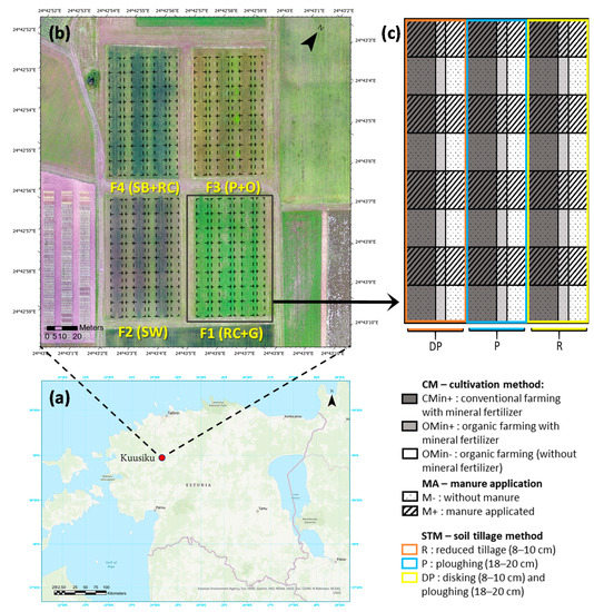
Figure 1.
(a) The study area located at the Kuusiku agriculture center, Estonia. (b) The RGB orthomosaic image from 30 May of the experimental layout fields with four crop types, i.e., (F1. (RC + G), F2. (SW), Field 3. (PO), and Field 4. (SB + RC)) (c) The VPT with three agricultural management practices (AMP): cultivation method (CM) with three levels (Cmin+, NPK 5-10-25 291 kg ha−1 (N-14 kg ha−1, P-13 kg ha−1, and K-60 kg ha−1); Cmin−, mineral fertilizer 240 kg ha−1 (K-60 kg ha−1, S-41 kg ha−1, M-14 kg ha−1); and Omin−), manure application (MA) with two levels (M+, manure 30,000 kg ha−1 (N-234 kg ha−1, P-20 kg ha−1, and K-216 kg ha−1), and M−), and soil tillage method (STM) with three levels (DP, P, and R) were conducted in this study.
2.2. UAS Image Acquisition
Figure 2 shows the workflow utilized to combine the UAS-based image collection, processing, sampling, and AutoML framework modified from [30]. A fixed-wing UAS eBee Plus (Sensefly Inc., Cheseaux–Lausane, Switzerland) equipped with GNSS post-processed kinematic (PPK) capabilities was deployed with a Parrot Sequoia multispectral sensor (version 1.2.1, Parrot, Paris, France). This UAS platform and sensor were used for image acquisition and captured imagery across four spectral bands: green (530–570 nm), red (640–680 nm), red-edge (730–740 nm), and near-infrared (770–810 nm). To facilitate seasonal image processing and AMP recognition, UAS images were captured over three timeslots in 2019 at the Kuusiku Research Center: 23 April (temperature: 16 °C, wind speed: 11 km h−1 S, sunny), 30 May (temperature: 19 °C, wind speed: 12 km h−1 WSW, overcast), and 10 July (temperature 20 °C, wind speed: 3.6 km h−1 NW, sun with minor cloud cover). The weather conditions in the 6 days prior to the image acquisition are displayed in Supplementary Figure S1. The originally designed flight time was 37 min and 30 s per task over an area of 65.8 hectares (with areas of interest 2.87 hectares in this study). However, depending on the weather conditions and wind speed of the day, the eBee flight time might have been slightly different from the number of battery replacements (the endurance of one battery was approximately 20–30 min). This data capture protocol was designed to represent the reflectance spectrum characteristics of crops during different growth stages. Flight-line overlap was set using a frontal image overlap of 80% and a lateral overlap of 75% with a target altitude of 120 m above ground level (AGL), resulting in a ground sampling distance (GSD) of 10 cm per pixel. All image data capture procedures were undertaken between the hours of 10 a.m. to 2 p.m. to guarantee the consistency of photo collection quality and to minimize lateral shading of crops within the VPT fields. An Airinov radiometric calibration target (Airinov, Paris, France) and a one-point calibration method [38] were used to enable post-flight radiometric correction of the multispectral imagery before each flight to remove dark current and lens vignetting effects while post-processing the image [39].
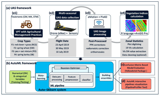
Figure 2.
The flowchart of the UAS and AutoML framework in this study. (a) The UAS framework, where (a1) Three types of AMPs were processed for four crop categories. (a2) The eBee plus with Parrot Sequoia multispectral sensor with the time series flight (April, May, and July) to collect spectral information from different crop periods. (a3) UAS image post-processed in SenseFly eMotion with PPK corrections and orthomosaics in Pix4D. (a4) 19 VIs calculation, segmentation and corresponding plot digital number (DN) extraction for AutoML modeling. (b) The Auto-sklearn framework constructed ML pipelines automatically, which were proposed by the Bayesian optimization method with warm-started meta-learning and joint with post hoc ensemble building approach to achieve robust performance (adapted from [30,40]). (c) Yellowbrick visualization package was conducted for AutoML model evaluation. (d) PipelineProfiler was conducted for AutoML interactive pipelines visualization tool allows the examination of the solution space of end-to-end ML pipelines.
2.3. UAS Image Processing
For pre-processing UAS images, we used SenseFly eMotion 3, applying differential correction data (RINEX) provided by the GNSS CORS (Continuously Operating Reference Station) of Estonia for post-processing kinematics (PPK) corrections [41]. PPK was reported to increase the higher horizontal and vertical geotagging accuracy when compared to ground control points (GCP) [42,43]. In our study, the UAS image corrections were decreased from 5 m error to under 0.06 m (less than one-pixel size). Pix4D v.4.3.31® (Pix4D SA, 1015 Lausanne, Switzerland) software was utilized to process and radiometrically correct (calibrated according to the variances between the measured value and target actual reflectance [38]) the imagery, as well as to generate the multispectral orthomosaics. These images were subsequently clipped with a one-meter inward buffer zone from each plot to represent only the extent of the area of the VPTs.
2.4. Vegetation Indices Calculation
In this study, nineteen VIs were chosen and calculated to address the issues of heterogeneous crop classes, soil types, and the current absence of valuable UAS referenced parameters in AMPs (see Table 1). More specifically, Datt4, SRre, NDVIre were selected due to their positive correlation with chlorophyll content [44,45,46]; MTVI, MSR, MSRre, RVIS, WDRVI [47,48,49,50,51] are known to be sensitive to variations in leaf area index (LAI); GDVI was used for better lower vegetal land cover estimates and characterization [52]; GIPVI was calculated for its potential in grassland communities detection [53]; GNDVI, NDVI, RTVIcore were utilized due to their high performance in crop above-ground biomass (AGB) estimation [54,55]; GDI, GRDI, and RDVI were included due to their ability to compensate for NDVI saturation problems, and the potential effects of soil and sun viewing geometry [56,57]; GRVI was applied for its sensitivity to soil moisture [58], SR for strongly correlated with comprehensive growth index (CGI) [59] and REGVI was included for its sensitivity to deviations in senescence and vegetation stress [60].

Table 1.
Descriptions and formulas of multispectral UAS derived VIs used in this study. The ρ R refers to the reflectance of the red band, ρ G refers to the reflectance of the green band, ρ REG refers to the reflectance of the red edge, and ρ NIR refers to the reflectance of the near-infrared.
2.5. Principal Component Analysis and VI Extraction
In this study, principal component analysis (PCA) was used to decrease the dimensionality of data through the calculation of a series of new variables, or principal components, through linear combinations of the original parameters [71]. PCA was employed as an exploratory data analysis (EDA) technique to describe the relationship between three different agricultural management types (CM, MA, and STM) and multispectral UAS-VIs. The PCA was used for testing whether or not it could improve the classification efficiency of AMPs. PCA was conducted using R version 4.0.2 [72] and the FactoMineR package [73]. For extraction of the digital number (DN) values from each VIs of four experimental fields (72 plots in each field), a total of 288 plots were digitized in ArcGIS Pro 2.6.3 [74]. As stated previously, a one-meter buffer zone was extended inwards from each plot boundary to address potential edge effects from agricultural management, and the average VIs were isolated and calculated. These extracted values were further used in this study when building ML algorithms and for AutoML assessment and evaluation.
2.6. AutoML Modeling with Auto-Sklearn
Auto-sklearn [30], a robust and efficient AutoML system first introduced in 2015 and upgraded in 2020 [75], was utilized in this study. Auto-sklearn is developed on the Python Scikit-learn machine learning package. It uses 15 classifiers, 14 feature pre-processing methods, and four data pre-processing methods, giving rise to a structured hypothesis space with 110 hyperparameters [76]. It improves on existing AutoML methods by automatically considering the previous performance on similar datasets, and by constructing ensembles from the models evaluated during the optimization process. At its core, this method combines the highly parametric ML framework with automatically constructed ML pipelines suggested by the Bayesian optimization method sequential model-based algorithm configuration (SMAC) [77]. SMAC can automatically construct ML pipelines that include feature selection (i.e., removing insignificant features), transformation (i.e., dimensionality reduction), classifier selection comprising support vector machines (SVM) [78], Random Forest (RF) [79], and other algorithms, hyperparameter optimization, etc. Subsequently, it then utilizes a Random Forest technique for swift cross-validation by evaluating one-fold at a time, while at the same time discarding poor-performing hyperparameter settings during early stages. It achieves competitive classification accuracy, in addition to novel pipeline operators that significantly increase classification accuracy on the datasets [80]. During the feature selection stage, any highly correlated VIs were removed to eradicate the influence of collinearity. This step was omitted here since Auto-sklearn deals with the low dimensional optimization problems [81].
In this study, all calculations were done in the open-source operating system LINUX with Intel Core i5-1035G1 CPU (1.00 GHz) and 16 GB RAM. For the AutoML framework, the steps described in [30] were followed, with some modifications for this study (Figure 2b). First, the system used a supplementary approach of extensively applied meta-learning methods to train machine learning models over statistical attributes of datasets and estimated the parameter of models that yielded the best precision [82]. Second, the system automatically built ensembles of the models considered by Bayesian optimization. Third, the system constructed a highly parameterized ML framework from high-performing classifiers and pre-processors implemented within the ML framework. Finally, the system performed broad empirical analysis using a diverse collection of datasets to demonstrate the resulting Auto-sklearn system outperformed preceding AutoML methods. The major AutoML parameter settings of this study are described in Table 2. Due to computational resource constraints and to test the efficiency of AutoML, we first limited the CPU time for each run to 60 s and the running time for evaluating a single model to 10 s as an example of rapid model selection. Subsequently, we then used a total of 1200 s with a 10-s single model computing time as a representative of the better processing of AutoML models. The data were analyzed separately according to the four crop fields (F1–F4), with each field containing 72 plots (n = 72) with a split in the training site and validation site (0.6/0.4) for classification modeling.
Table 2.
The AutoML main parameters and descriptions used in this study.
A recent review study of supervized ML methods applied in land-cover image classification disclosed that Random Forest (RF), support vector machine (SVM), and artificial neural network (ANN) classifiers were among the most commonly used ML techniques from 220 related articles [83]. Therefore, in this study, these popular ML classifiers were selected for comparison against the accuracy performance of AutoML (with 60-s run, and 1200-s run of Auto-sklearn). These algorithms were programmed in Python by the robust ML library Scikit-learn (0.24.2) [76] with the perimeter setting as following: sklearn.ensemble.RandomForestClassifier (100 trees; min_samples_split (2); leaf_node (1)); sklearn.svm.SVC (cost (C = 500); gamma (0.5); epsilon (0,01)), and sklearn.neural_network.MLPClassifier (alpha (0.00005); the maximum number of iterations (100,000)) The parameters not mentioned were computed as default settings from Scikit-learn, and for the accuracy, calculation referring to Table 3.
Table 3.
The confusion matrix-based accuracy evaluation equations used throughout this study.
2.7. AutoML Model Evaluation and Visualization
For the visualization and evaluation of the Auto-sklearn model, the workflow included, in general, multiple iterations through feature engineering, algorithm selection, and hyperparameter tuning [84]. In this study, an open-source visual steering tool Yellowbrick visualization package (essentially a wrapper for the Sklearn documentation) was conducted for AutoML evaluation [85]. Yellowbrick contributes to assessing the stability and predictive values of ML models and delivers visualizations for our AutoML classification models. The accuracy evaluation based on the confusion matrix system of the AutoML classification parameters were defined as follows: true positive (TP), false positive (FP), true negative (TN), and false negative (FN), which have been well described in [86]. The equations used in this study are described in Table 3. The derived receiver operating characteristic curve (ROC) graph with the x-axis showing FPR and the y-axis showing TPR was used in this study to show the relationship among specificity and sensitivity for each possible cut-off [87] and the area under the curve (AUC) ranges from 0 to 1 to visualize the trade-off between the classifier’s sensitivity and specificity [87,88]. Macro- and micro-averaging ROC were calculated to evaluate overall classifier performance in multi-class problems. In this approach, the ROC curve was calculated anew, based upon the true positive and false positive rates for all dataset (by weighting curves by the relative frequencies of the dataset and then averaging them) [89,90]. In addition, the precision–recall curve (PR) was calculated for different probability thresholds. PR curves were conducted in cases where there was an imbalance in the observations between the classes [91] as another classification evaluation standard to assist with the ROC curve. The prediction errors (confusion matrix) and classification report that displays precision, recall, and F1-score [92] (Table 3) per class as a heatmap in our study.
Alternatively, even though the AutoML framework facilitates the construction of models, given their black-box nature, the complication of the underlying algorithms and the large number of pipelines they derive leads to the reduced trust of AutoML pipelines systems [93]. Therefore, in our study, PipelineProfiler [94] was conducted for AutoML pipelines visualization. PipelineProfiler is a SOTA in visual analytics for AutoML interactive visualization tool that allows the examination of the solution space of end-to-end ML pipelines. It offers a recovering understanding of how the AutoML algorithms are generated and the perceptions of how they can be optimized. As the outcome of the interactive AutoML pipeline matrix plots, where illustrated Pipeline flowchart, primitives used by the pipelines; one-hot-encoded hyperparameters for the primitive across pipelines; the accuracy ranking; primitive contribution view; and the class balancing of correlation score with accuracy. These calculations and expressions are clearly detail described in the [94] article.
3. Results
3.1. The AMPs Observation in VPTs and VIs Calculation
Figure 3 displays the observation of onsite crop VPTs (i.e., Field 1 (F1) (Figure 3a) and Field 2 (F2) (Figure 3b) with CM treatments) and one of the VIs (NDVI; Figure 3c) captured on 10 July from F1 and F2. It can be observed from the onsite AMPs treatment photographs of F1 and F2 in July that it was not readily distinguishable. In addition, it can be seen from the NDVI image that the heterogeneity within the plot may be caused by edge effects or uneven fertilization. For this reason, we used the plot average value considering the pixels inward boundary clipping to decrease the noise.
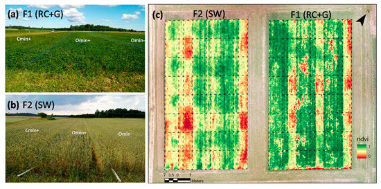
Figure 3.
Interpretation diagrams representing onsite crop VPTs and the calculation of VIs per the image captured on 10 July (a) Field 1: red clove + grass (RC + G) with CM treatment. (b) Field 2: Spring wheat (SW) field with CM treatment. (c) Normalized Difference Vegetation Index (NDVI) image captured of F1 (RC + G) and F2 (SW) VPT.
3.2. Monthly PCA Analysis in Various Crop Growth Periods
PCA was conducted as the first step of data exploration in this study to gain an understanding of the relationship between VIs and different AMP categories during the three flight periods (April, May, and July) with their corresponding growing stages (Figure 4). The results showed that on 30 May and 10 July, the PC1 and PC2 captured most of the variation from the F1 to F4 fields with 98.3%, 98.7%, 97.3%, and 97.6%, respectively, on 30 May (Figure 4b), and with 98.7%, 94.0%, 95.4%, and 95.4%, respectively, on 10 July (Figure 4c); followed by 23 April (Figure 4a). In addition, during the three flight periods, the PCA results in May and July provide better separation of the three AMP categories throughout the four crop cultivation areas based on the colored concentration ellipses where the sizes were determined by a 0.95-probability level. In terms of the AMP category, the subclasses of CM (Cmin+ Cmin+ and the other two categories) and MA (M+ and M−) seemed easier for non-overlapping AMP clustering, followed by STM. In terms of crop types, F1 (SW) were better clustered in April, while F2 (SW), F3 (P + O), and F4 (SB + RC) were better clustered in May or July. Given the better clustering performance in May, follow-up AutoML analysis was conducted on the UAS-VIs data of this month. In general, feature selection (finding the most relevant spectral bands) and extraction (reduced set of new significant variables) are commonly used to solve the collinearity and overfitting problems in the dimensionality reduction process [95]. However, after our test results, using PCA, 95% feature extraction in our preliminary experiments could not significantly improve the classification efficiency. Therefore, these PCA results were simply used as a reference basis for AutoML classification.
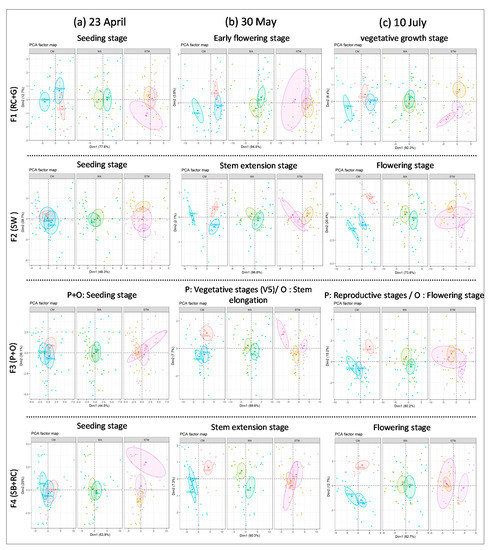
Figure 4.
PCA biplot of 19 VI variables (n = 72) of each crop field on (a) 23 April, (b) 30 May, and (c) 10 July. Each biplot shows the PCA individuals (three AMPs) (i.e., CM (Cmin, Omin+, Omin−), MA (M+, M−), STM (DP, P, R)) of the first (x-axis: PC1 score) and second (y-axis: PC2 score) principal components (the variation explained by the dimensions are shown on the axes); four crop categories (F1–F4) and its corresponding growing stage from top to bottom. Colored concentration ellipses (size determined by a 0.95-probability level) show the observations grouped by marked AMP sub-classes.
3.3. AutoML ROC and AUC Evaluation of AMP Recognition in May
The different subclasses and average results of ROC/AUC were calculated for evaluation of the AutoML performance for the AMP classification ability in UAS-VIs that were captured in May (Figure 5), where AUC values were categorized in this study as AUC = 0.5: no discrimination; 0.7 ≤ AUC ≤ 0.8 (acceptable discrimination); 0.8 ≤ AUC ≤ 0.9 (excellent discrimination); 0.9 ≤ AUC ≤ 1.0 (outstanding discrimination) [87].
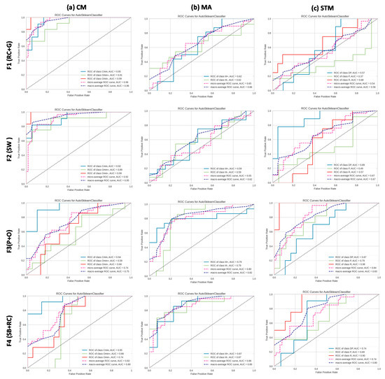
Figure 5.
ROC curves and AUC of the AutoML classification corresponding to the subclasses within the AMPs for the acquisition of the UAS-VIs DN in May. From left to right, the ROC curves computed on (a) CM (Cmin+ (blue lines), Omin+ (green lines), Omin− (red lines)); (b) MA [M+ (blue lines), M− (green lines)]; (c) STM (DP (blue lines), P (green lines), R (red lines)); and their micro (pink dotted line) and macro (dark blue dotted line) average performance. Four crop categories (F1–F4) from top to bottom.
The AutoML results showed that the micro-average ROC of CM’s classification resulted in F1 (RC + G) and F2 (SW) being higher (AUC = 0.95, and 0.92, respectively). Especially in the subclass Omin−, the AUC both reached 0.99 for the micro-average ROC, followed by F4, and F3 (P + O), with 0.86 and 0.75, respectively) (Figure 5a). On the contrary, MA classification results showed that the micro-average AUC in F3 and F4 were higher (AUC = 0.83, and 0.89, respectively), followed by F1 (AUC = 0.71). F2 performance for MA was the worst (AUC = 0.51), with no discrimination ability (Figure 5b). In contrast, STM classification results were generally poor, with better results only present in F3, while other fields have larger divergence in classification results under the sub-class (DP, P, and R), as shown in Figure 5c). Overall, the AutoML classification ability from UAS-VIs of CM was the best, followed by MA and STM.
3.4. AutoML Precision–Recall, Prediction Error, and Classification Report of CM Recognition
Among the classification results of AMPs in May (Figure 5) of four crop types, CM yielded the best ROC/AUC overall performance. Therefore, we used the precision–recall (PR) curves, prediction error, and classification report plots to gain an in-depth understanding of the classification status of CM treatments (Figure 6).
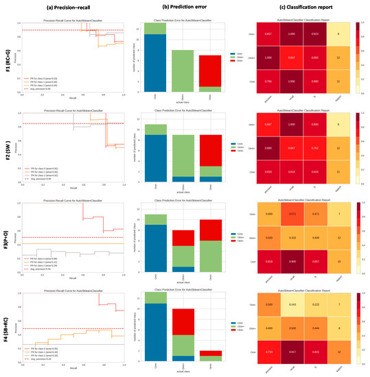
Figure 6.
The evaluation of AutoML classification of AMPs from the acquisition of the UAS-VIs DN in May. (a) Precision–recall, where the class 0, 1, 2 equals to Cmin+, Omin+, and Omin−, respectively (b) Prediction error (confusion matrix), the X-axis represents the three subclass form CM result in May, and the Y-axis represents the type (with color), and the number of correct or incorrect estimates., and (c) Classification report lists the precision, recall, and F1-score per class as a heatmap for overall comprehensive evaluation results. The calculation methods used in this figure are shown in Table 3.
The PR curve of F4 CM shows the trade-off between a classifier’s precision performance from UAS VIs in May (Figure 6a), where a model with perfect performance is depicted at the coordinate of (1,1). A curve that tends towards the (1, 1) coordinate represents a well-performing model, whereas a no-skill classifier is depicted as a horizontal line on the plot with a precision that is proportional to the number of positive examples in the dataset. For a balanced dataset, this value ought to be 0.5 [96]. The results showed that the classifications of Fields 1 and 2 were promising, their average PR being 0.90 and 0.85, respectively, while the results of F3 and F4 were poor (0.50 and 0.49). We can further discover from the prediction error graph (Figure 6b) in F3 and F4 that the judgment error of Cmin+ was low, and the confusions of Omin+ and Omin− were more common. We can also compare the precision, recall, and F1-score results of various cultivation method sub-classes to evaluate the classification accuracy from the heatmap (Figure 6c).
3.5. AutoML Pipeline Visualization
An interactive AutoML visualization tool PipelineProfiler was used in this study. Figure 6 shows the CM classification results across four crop fields in May with the accuracy performance of AutoML pipelines running time set at 60 s, and the primitive comparison against the others, and the real-time hyperparameter selection strategy (Figure 7). The results demonstrated that the best classifier found for Field 1 was linear discriminant analysis (LDA) [97] (Figure 7a), for Field 2, it was the Extra Trees Algorithm [98] (Figure 7b), for Field 3, it was LDA (Figure 7c), and Random Forest (RF) for Field 4 (Figure 7d), with each of their hyperparameters found by AutoML also being represented in the figures.
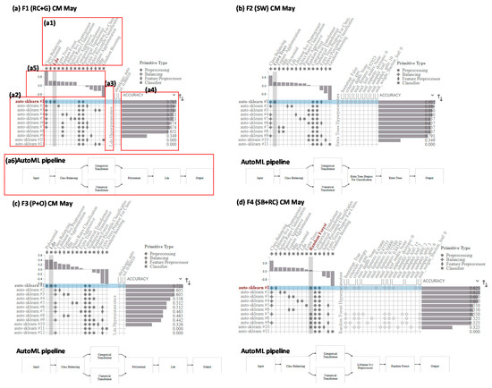
Figure 7.
The interactive AutoML pipeline matrix plots with running time-limited setting 60 s sorted by accuracy performance (a–d), (a) Field 1 pipeline matrix with the Top1 classifier LDA, where (a1) illustrated Primitives (in columns) used by the pipelines (a2) (in rows, the blue line showed the best accuracy rank); (a3) one-hot-encoded hyperparameters (in columns) for the primitive across pipelines, (a4) the AutoML pipeline with the accuracy ranking; (a5) Primitive contribution view, showing the correlations between primitive usage and pipeline scores—in a5 displays that class balancing has the highest correlation score with accuracy; (a6) Step by step AutoML Pipeline flowchart. The ML box before Output represents the classifier used by this set of algorithms (in a6 LDA as the classifier) (b–d) Fields 2, 3, and 4 interactive pipeline matrix sort by AutoML accuracy performance with the chosen hyperparameters (top 1 was listed).
3.6. Comparison of Performance between AutoML and Other Machine Learning Technologies
Based on the large calculations and multiple classifier selections that were required during the initial stage of AutoML computations, the processing time setting of 60 s may not completely reflect the performance power of AutoML. To evaluate the effects of AutoML processing time, we adjusted the times to 1200 s and 60 s (original running time) and considered the AMPs’ classification accuracy with RF, SVM, and ANN algorithms (Table 4). The results demonstrated that under the permutation and combination of ML algorithms included in AutoML, classification accuracy did not perform well in 60 s of computing time. Furthermore, performance was the worst in F1 CM, F2 STM, and F3 CM classifications compared to RF, SVM, and ANN. However, as processing time was increased to 1200 s, the classification accuracy of AutoML in AMPs was shown to improve. The results also indicated that overall AutoML (1200 s) and RF classifiers produced 5 and 3 best classification accuracy in AMPs, respectively (in black bold) and did not produce the worst accuracy values (in bold red) in any instances. Regarding SVM and ANN, the classifiers performed the best in 3 and 5 cases, respectively. However, these methods consistently produced low-performing classifiers compared to other AMPs.
Table 4.
The AMPs classification accuracy comparison of AutoML and three other popular applied ML (RF, SYM, and ANN) algorithms in UAS.
4. Discussion
This paper is the first study to use an auto-learning system, with UAS multispectral-derived VIs, for agricultural classification purposes. The study provides a novel AutoML framework across multiple AMP activities and presents a UAS and ML methodology optimized for future PA and crop phenotyping research.
4.1. Applicability and the Impact of the AutoML Method in UAS
In this study, we employed a SOTA, open-sourced AutoML framework for automatic, rapid multispectral image classification strategies and assistance in optimizing problematic hyperparameter adjustments. This technology brings several benefits and enhances the application of UAS for environmental and ecological research classification tasks.
First, UAS related classification research publications have significantly increased within recent years, with over a hundred articles developed since 2017. This substantial adoption of UAS related classification approaches demonstrates its impact and the mounting interest in such research issues [99]. Our UAS-AutoML framework may also be implemented in other UAS classification research, such as research employing multi-sensors (i.e., thermal, visible light, hyperspectral, radar or light detection and ranging (Lidar) sensors) across a range of contemporary agriculture classification activities (i.e., weed management [100,101], crop phenotyping [9,102,103,104], disease monitoring [105,106], etc.), as well as research focused on ecological classification schemes, multispectral-based plant community mapping options [107], and coastal wetland vegetation classification results [108].
Second, the AutoML framework quickly provided usable classifiers and hyperparameter selections for unknown UAS classification tasks and parameter selection. For example, in the current study, the parameters and applicable classifiers of AMPs were unknown a priori. However, it provided a promising and efficient performance rating for classifiers for inclusion in modeling selection. As the results of Figure 6 show, LDA (Figure 7a,c) and Extra Trees (Figure 7b) were chosen as the best classifiers corresponding to the VPT fields of the AMP recognition task. These ML methods have been less applied and referenced in the field of UAS [83]. These findings clearly illustrate that AutoML has the potential to locate alternative ML approaches that might customarily be ignored by investigators with unknown classification subjects.
Third, the operational efficiency of AutoML classifiers can be given a time limit and gives the researcher the flexibility to find the most suitable formula within the required time. In general, a longer time setting allows for increasingly accurate results with additional classifier combinations. Since our experiments did not involve substantially large datasets, the focus was put on time setting close to the minimum limit of AutoML calculation (60 s of total CPU operation (this can be up to 3000 s) and 10 s of a single ML algorithm computation) to highlight the flexibility and rapid performance of AutoML.
Finally, within our research, the latest released AutoML interactive visualization system PipelineProfiler was employed and assisted in the screening of classifiers and the reference of fine-tuning parameters when analyzing UAS data. This interaction included adjustable time, accuracy ranking, and selection of hyperparameters in response to the requirement of customized UAS modeling. Our results showed that AutoML computations within 60-s-run produced between 11 and 12 pipelines (Figure 7), which might offer a beneficial foundation for providing adequate outcomes in most cases with minimal attempts and time.
4.2. The Impact of Algorithm Selection, Cultivated Period, and Crop Types in AutoML AMP Recognization
In terms of algorithm selection in our AMP classification results, different classifiers were suggested by AutoML as the best performances even within the same AMP category for different crop types (Figure 7). We can conclude that applying AutoML in UAS-derived multispectral VI data allowed for the consideration of a variety of algorithm combinations to meet the complexity of the VPT field. We also compared the three most used ML algorithms (RF, SVM, and ANN) in the UAS classification fields with AutoML algorithms (Table 4). The overall performance showed that AutoML (with 1200-s CPU duration) provided the five best (or equal best) accuracy performances (shown in bold black in Table 4). Interestingly, in all tests, the AutoML (1200) and RF methods were never found to be the worst-performing methods (shown in bold red). Moreover, when using the ANN method, despite providing five of the best classification accuracy results, this method also included five of the worst performance results. Similar outcomes were observed regarding the SVM and AutoML 60-s runs.
From our results, we can deduce that increasing the computing time has the potential to improve the accuracy and stability of AutoML classification performance under certain AMPs conditions. However, it also highlights the potential to include AutoML methods in the computation of common classification problem-solving. Similar ranks were shown in a study that compared the results of the numerous classifiers with Auto-sklearn, where the RF classifier presented the strongest performance, and SVM showed robust performance for some datasets [30]. Since the Auto-sklearn classifiers are based on Scikit-learn as a blueprint, it should theoretically capture the hyperparameters of the RF algorithm on what was selected for Table 4. Despite the strong performance of AutoML (1200 s), there were still several results that indicated the inferiority of AutoML (1200 s) when compared to the RF classifier (i.e., Field 1 MA; Field 3 MA, and STM). Moreover, in a few cases, the accuracy of AutoML (1200 s) was even lower than the calculation result of the 60-s set (i.e., Field 1 MA, Field 3 STM, and Field 4 CM). It may be that the algorithm computations involve different factors other than accuracy, and the model it uses to tune the parameters actively tries to avoid overfitting. This will possibly lead to the situation where the most accurate model, on the testing or training data, will not be the one that can generalize the best on real data. In addition, developers from the Auto-sklearn team have previously described that during the ensemble selection phase, the methods can add numerous substandard models to the final ensemble, and unregularized selection may lead to overfitting with a small number of candidate models [40]. This result shows that there is still room for improvement regarding AutoML calculation methods in the future.
In terms of cultivated period and crop type, according to the monthly performance of different crop growth stages, the PCA results indicated that the VPT with better clustering performance occurred during the flight in May, with a confidence level of 0.95 (Figure 4b). In this regard, this flight period was further used for our AMPs’ classification study. Conversely, in the case of more homogeneous crop types (Field 3 (WS)), and despite the promising classification result in CM, the results of MA and STM were not as effective as other crops (Figure 5 and Figure 6). These results may suggest that even with higher heterogeneity of cultivation within the plots (i.e., F1, F3, and F4), it appears not necessarily to affect the classification ability. However, concerning the Field 3 results from the PCA in May (stage of stem elongation) and July (stage of flowering), the MA clustering ability was better with a 0.95 confidence level in both months, and the accuracy was later improved from the classification analysis. The results of our study have demonstrated that, although the feature selection stage of AutoML is a black box, we can still preliminarily determine the potential predictive ability of the AutoML model based on PCA result and reduce the cost of period selection as we did in this study. In addition, this study has contributed evidence to the classification obstacles in the case of STM that may be caused by the orientation of images taken over vegetation or soil with uniform texture and re-cursive pattern, sub-optimal flight configuration [109], or unflavored VIs selection. Some studies also suggest that the use of grey-level co-occurrence matrix (GLCM)-based texture information [100,110], semantic segmentation [111], or edge computing [112] can improve the accuracy of UAS-ML classification in the crop categories. This may be an applicable technology for AMPs classification in the future. The applicability and optimization of this framework, and the visualization of feature importance, required the optimization of the AutoML programmers and UAS application feedback to improve.
Currently, multispectral indices have been effectively applied in some AMP image analysis studies with the color, texture, and shape factors of the agricultural land at the satellite level. These include conservation tillage methods identification [113] and agriculture landscapes with pixel-based or object-based classification tasks [114,115]. AMPs application are indispensable for environmental monitoring and for facilitating the agricultural decision-making process, regarding the adoption practices proposed by growing conservation agriculture demand [116], and for its potential upscaling ability to accelerate land cover classification studies. Recently, combining commonly adopted management practice with UAS multispectral-VIs research has gradually gained attention and has been applied to cotton and sorghum fields [117]. In our study, the effective application of UAS sensors to recognize multiple AMP categories has been shown. More specifically, an UAS-AutoML approach can improve the classification ability under specific crop AMPs, highlighting that, in this study site, classification performed better in CM, with overall classification performance followed by MA and STM.
4.3. The Limitations of Our Method
In this study, not all classifiers computed within the Auto-sklearn system were able to be backtracked and reviewed to investigate the individual feature importance rankings of VIs, which has limitations in terms of their ability to assist in the selection of suitable VIs for AMPs classification tasks. However, our efforts to achieve a wide-ranging and well-considered predictor collection through a variety of VI combinations may lead to performance improvements. This study may also be limited by the location, crop categories selected, and varieties present at the study site. However, these issues can be simply addressed by including a wider range of VPT at multiple study sites and across a greater diversity of crop types in future investigations. Due to the characteristic complexity and repeatability of VPT, we need to recognize that the small sample size, and the potential interaction effects between trials, were not fully addressed. A potential solution worth pursuing may be to increase the VPT sampling size and/or enhance the segmentation number of each plot, ultimately increasing the training samples for AutoML calculation. Currently, the applicability of the AutoML framework will still require more UAS-based tests in the future to demonstrate its true potential and effectiveness.
5. Conclusions
First, our study demonstrated a novel UAS technology and a state-of-the-art AutoML framework across multiple AMP tasks through non-destructive and cost-effective approaches. The scientific merit of this article lay in utilizing artificial intelligence to replace the judgment of the human for UAS classification analysis with its automated data pre-processing, model selection, feature engineering, and hyperparameter optimization capabilities. Furthermore, it provided innovative insights into agricultural management practices and accelerated the intellectualized progress of the in-field monitoring UAS system and established future crop phenotyping abilities. In our study, AutoML embodied “learning how to learn” for any given UAS subject; and it is the first study of its kind to apply an auto-learning system for AMP classification tasks in multispectral-derived VI data.
Second, in this study, we employed an AutoML workflow combined with two innovative visualization tools. We performed three multispectral-UAS flights at the farm-scale, under the four crop types (RC + G, SW, PO, and SB + RC) of VPT within three AMPs (CM, MA, and STM) treatments. In addition, we compared AutoML performance with those of three widely used ML methods. The ML comparison analysis results showed AutoML achieved the most overall classification accuracy numbers after 1200 s of calculation and without any of the worst-performing classifications of the given datasets. In terms of AMPs classification, the best recognized period for data capture occurred in the crop vegetative growth stage (in May of Estonia). The result demonstrated that CM yielded the best performance in terms of treatment, followed by MA, and STM; the last was shown to be the worst-performing treatment. These conclusions may be attributed to the low heterogeneity of the spectral reflectance value in the corresponding AMP treatment.
Third, the flexibility of fixed-wing imaging technology provides longer flight durations and thus allows for larger applications, such as commercial farmland, grasslands, forests, etc. Furthermore, the multispectral dataset produces various precise VIs without the need for any supplementary sensors, which reduces measurement errors and significantly reduces costs. In addition, given the AutoML’s open-sourced platform and the powerful capabilities of automation, the complexities surrounding parameter selection in machine learning are greatly reduced, while it also has the potential to select long-ignored but highly efficient ML algorithms. Regarding the choice of AutoML systems or interfaces, although many of them have been developed successively (i.e., Auto-sklearn, H2O AutoML, AutoKeras), it is necessary to identify whether their subsequent updates and revisions keep up to date with current times.
Lastly, this UAS-AutoML solution has the potential to be implemented across a variety of other UAS classification research, such as contemporary agricultural classification methods, multispectral-based plant community mapping, ecological or wetland plant community recognition. Other remote sensing classification methods that lack algorithm and hyperparameter backgrounds may also be considered and benefited from our findings and insights.
In summary, our study, the UAS application particularly focused on the adoption and application of AutoML method across a diverse range of agricultural environmental assessment and management applications. Our approach demonstrated that UAS based on our AutoML framework, can recognize multiple agricultural management practices under certain conditions and that the integration of UAS technologies, geoprocessing methods, and automatic systems are vital tools for increasing the knowledge of plant–environment interactions within the management of crops. The framework also considerably contributes towards the simplified advancement of image-driven analytical pipelines for current VPT systems used in most countries. At the end of preparing this study, the Google Cloud AutoML also came out in 2019 for image-recognition use cases [118], showing that automatic learning will drive a non-negligible impact in the UAS field and provide new insight into the potential for remotely sensed solutions to field-based and multifunctional platforms for the demands of precision agriculture in the future.
Supplementary Materials
The following are available online at https://www.mdpi.com/article/10.3390/rs13163190/s1, Figure S1: Daily climograph of the study area (Kuusiku) during the flying period, including the previous 6 days (a. 17–23 April, b. 24–30 May, and c. 4–10 July) in 2019. Blue bars and the red line represent the daily average of rainfall and temperature, respectively.
Author Contributions
All authors contributed significantly to the work presented in this paper. All authors have read and agreed to the published version of the manuscript.
Funding
This research was funded by the European Regional Development Fund within the Estonian National Programme for Addressing Socio-Economic Challenges through R&D (RITA): L180283PKKK and the Doctoral School of Earth Sciences and Ecology, financed by the European Union, European Regional Development Fund (Estonian University of Life Sciences ASTRA project “Value-chain based bio-economy”).
Institutional Review Board Statement
Not applicable.
Informed Consent Statement
Not applicable.
Data Availability Statement
The data presented in this study are available on request from the corresponding author. The data are not publicly available due to the data size.
Acknowledgments
We give great thanks to the community that develop and maintain the scikit-learn framework, as well as the Auto-sklearn interface developed at the University of Freiberg. In addition, this work was supported by Kuusiku Variety Testing Centre, Estonia, with the tests carried out by order of Agricultural Board. Information about variety listings are currently available in www.pma.agri.ee.
Conflicts of Interest
The authors declare no conflict of interest.
References
- Mulla, D.J. Twenty five years of remote sensing in precision agriculture: Key advances and remaining knowledge gaps. Biosyst. Eng. 2013, 114, 358–371. [Google Scholar] [CrossRef]
- Tripicchio, P.; Satler, M.; Dabisias, G.; Ruffaldi, E.; Avizzano, C.A. Towards Smart Farming and Sustainable Agriculture with Drones. In Proceedings of the 2015 International Conference on Intelligent Environments, IEEE, Rabat, Morocco, 15–17 July 2015; pp. 140–143. [Google Scholar] [CrossRef]
- Herwitz, S.R.; Johnson, L.F.; Dunagan, S.E.; Higgins, R.G.; Sullivan, D.V.; Zheng, J.; Lobitz, B.M.; Leung, J.G.; Gallmeyer, B.A.; Aoyagi, M.; et al. Imaging from an unmanned aerial vehicle: Agricultural surveillance and decision support. Comput. Electron. Agric. 2004, 44, 49–61. [Google Scholar] [CrossRef]
- Zhang, C.; Kovacs, J.M. The application of small unmanned aerial systems for precision agriculture: A review. Precis. Agric. 2012, 13, 693–712. [Google Scholar] [CrossRef]
- Tsouros, D.C.; Bibi, S.; Sarigiannidis, P.G. A Review on UAV-Based Applications for Precision Agriculture. Information 2019, 10, 349. [Google Scholar] [CrossRef]
- Xiang, H.; Tian, L. Development of a low-cost agricultural remote sensing system based on an autonomous unmanned aerial vehicle (UAV). Biosyst. Eng. 2011, 108, 174–190. [Google Scholar] [CrossRef]
- Raeva, P.L.; Šedina, J.; Dlesk, A. Monitoring of crop fields using multispectral and thermal imagery from UAV. Eur. J. Remote Sens. 2018, 52, 192–201. [Google Scholar] [CrossRef]
- Sankaran, S.; Khot, L.R.; Carter, A.H. Field-based crop phenotyping: Multispectral aerial imaging for evaluation of winter wheat emergence and spring stand. Comput. Electron. Agric. 2015, 118, 372–379. [Google Scholar] [CrossRef]
- Yang, G.; Liu, J.; Zhao, C.; Li, Z.; Huang, Y.; Yu, H.; Xu, B.; Yang, X.; Zhu, D.; Zhang, X.; et al. Unmanned Aerial Vehicle Remote Sensing for Field-Based Crop Phenotyping: Current Status and Perspectives. Front. Plant Sci. 2017, 8, 1111. [Google Scholar] [CrossRef]
- Araus, J.L.; Cairns, J. Field high-throughput phenotyping: The new crop breeding frontier. Trends Plant Sci. 2014, 19, 52–61. [Google Scholar] [CrossRef]
- Andrade, J.; Edreira, J.I.R.; Mourtzinis, S.; Conley, S.; Ciampitti, I.; Dunphy, J.E.; Gaska, J.M.; Glewen, K.; Holshouser, D.L.; Kandel, H.J.; et al. Assessing the influence of row spacing on soybean yield using experimental and producer survey data. Field Crop. Res. 2018, 230, 98–106. [Google Scholar] [CrossRef]
- Laidig, F.; Piepho, H.-P.; Drobek, T.; Meyer, U. Genetic and non-genetic long-term trends of 12 different crops in German official variety performance trials and on-farm yield trends. Theor. Appl. Genet. 2014, 127, 2599–2617. [Google Scholar] [CrossRef]
- Lollato, R.P.; Roozeboom, K.; Lingenfelser, J.F.; Da Silva, C.L.; Sassenrath, G. Soft winter wheat outyields hard winter wheat in a subhumid environment: Weather drivers, yield plasticity, and rates of yield gain. Crop. Sci. 2020, 60, 1617–1633. [Google Scholar] [CrossRef]
- Zhu-Barker, X.; Steenwerth, K.L. Nitrous Oxide Production from Soils in the Future: Processes, Controls, and Responses to Climate Change, Chapter Six. In Climate Change Impacts on Soil Processes and Ecosystem Properties; Elsevier: Amsterdam, The Netherlands, 2018; pp. 131–183. [Google Scholar] [CrossRef]
- De Longe, M.S.; Owen, J.J.; Silver, W.L. Greenhouse Gas Mitigation Opportunities in California Agriculture: Review of California Rangeland Emissions and Mitigation Potential; Nicholas Institute for Environ, Policy Solutions Report; Duke University: Durham, NC, USA, 2014. [Google Scholar]
- Zhu-Barker, X.; Steenwerth, K.L. Nitrous Oxide Production from Soils in the Future. In Developments in Soil Science; Elsevier: Amsterdam, The Netherlands, 2018; Volume 35, pp. 131–183. [Google Scholar] [CrossRef]
- Crews, T.; Peoples, M. Legume versus fertilizer sources of nitrogen: Ecological tradeoffs and human needs. Agric. Ecosyst. Environ. 2004, 102, 279–297. [Google Scholar] [CrossRef]
- Munaro, L.B.; Hefley, T.J.; DeWolf, E.; Haley, S.; Fritz, A.K.; Zhang, G.; Haag, L.A.; Schlegel, A.J.; Edwards, J.T.; Marburger, D.; et al. Exploring long-term variety performance trials to improve environment-specific genotype × management recommendations: A case-study for winter wheat. Field Crop. Res. 2020, 255, 107848. [Google Scholar] [CrossRef]
- Gardner, J.B.; Drinkwater, L.E. The fate of nitrogen in grain cropping systems: A meta-analysis of 15N field experiments. Ecol. Appl. 2009, 19, 2167–2184. [Google Scholar] [CrossRef]
- Drinkwater, L.; Snapp, S. Nutrients in Agroecosystems: Rethinking the Management Paradigm. Adv. Agron. 2007, 92, 163–186. [Google Scholar] [CrossRef]
- van Ittersum, M.K.; Cassman, K.G.; Grassini, P.; Wolf, J.; Tittonell, P.; Hochman, Z. Yield gap analysis with local to global relevance—A review. Field Crop. Res. 2013, 143, 4–17. [Google Scholar] [CrossRef]
- Nawar, S.; Corstanje, R.; Halcro, G.; Mulla, D.; Mouazen, A.M. Delineation of Soil Management Zones for Variable-Rate Fertilization. Adv. Agron. 2017, 143, 175–245. [Google Scholar] [CrossRef]
- Chlingaryan, A.; Sukkarieh, S.; Whelan, B. Machine learning approaches for crop yield prediction and nitrogen status estimation in precision agriculture: A review. Comput. Electron. Agric. 2018, 151, 61–69. [Google Scholar] [CrossRef]
- Zhang, W.; Zhang, Z.; Chao, H.-C.; Guizani, M. Toward Intelligent Network Optimization in Wireless Networking: An Auto-Learning Framework. IEEE Wirel. Commun. 2019, 26, 76–82. [Google Scholar] [CrossRef]
- He, X.; Zhao, K.; Chu, X. AutoML: A survey of the state-of-the-art. Knowl. Based Syst. 2020, 212, 106622. [Google Scholar] [CrossRef]
- Mendoza, H.; Klein, A.; Feurer, M.; Springenberg, J.T.; Hutter, F. Towards Automatically-Tuned Neural Networks. In Proceedings of the Workshop on Automatic Machine Learning, New York, NY, USA, 24 June 2016. [Google Scholar]
- Zöller, M.-A.; Huber, M.F. Benchmark and Survey of Automated Machine Learning Frameworks. J. Artif. Intell. Res. 2021, 70, 409–472. [Google Scholar] [CrossRef]
- Yao, Q.; Wang, M.; Chen, Y.; Dai, W.; Hu, Y.Q.; Li, Y.F.; Tu, W.W.; Yang, Q.; Yu, Y. Taking the Human out of Learning Applications: A Survey on Automated Machine Learning. arXiv 2018, arXiv:1810.13306. [Google Scholar]
- Thornton, C.; Hutter, F.; Hoos, H.H.; Leyton-Brown, K. Auto-WEKA: Combined Selection and Hyperparame-ter Optimization of Classification Algorithms. In Proceedings of the ACM SIGKDD International Conference on Knowledge Discovery and Data Mining, Chicago, IL, USA, 11–14 August 2013; pp. 847–855. [Google Scholar]
- Feurer, M.; Klein, A.; Eggensperger, K.; Springenberg, J.T.; Blum, M.; Hutter, F. Auto-sklearn: Efficient and Robust Automated Machine Learning. In Proceedings of the Advances in Neural Information Processing Systems, Vancouver, BC, Canada, 8–14 December 2019; pp. 113–134. [Google Scholar] [CrossRef]
- Remeseiro, B.; Bolon-Canedo, V. A review of feature selection methods in medical applications. Comput. Biol. Med. 2019, 112, 103375. [Google Scholar] [CrossRef]
- Babaeian, E.; Paheding, S.; Siddique, N.; Devabhaktuni, V.K.; Tuller, M. Estimation of root zone soil moisture from ground and remotely sensed soil information with multisensor data fusion and automated machine learning. Remote Sens. Environ. 2021, 260, 112434. [Google Scholar] [CrossRef]
- Ledell, E.; Poirier, S. H2O AutoML: Scalable Automatic Machine Learning. In Proceedings of the 7th ICML Workshop on Automated Machine Learning, Vienna, Austria, 17 July 2020; Available online: https://www.automl.org/wp-content/uploads/2020/07/AutoML_2020_paper_61.pdf?fbclid=IwAR2QaAJWDbgi1jIfnhK83x2g3hV6APfvTZoeUblcf4q44wxqT1z5oRTiEVo (accessed on 20 October 2020).
- Koh, J.C.O.; Spangenberg, G.; Kant, S. Automated Machine Learning for High-Throughput Image-Based Plant Phenotyping. Remote Sens. 2021, 13, 858. [Google Scholar] [CrossRef]
- Jin, H.; Song, Q.; Hu, X. Auto-Keras: An Efficient Neural Architecture Search System. In Proceedings of the ACM SIGKDD International Conference on Knowledge Discovery and Data Mining, Anchorage, AL, USA, 4–8 August 2019. [Google Scholar] [CrossRef]
- Komer, B.; Bergstra, J.; Eliasmith, C. Hyperopt-Sklearn: Automatic Hyperparameter Configuration for Scikit-Learn. In Proceedings of the 13th Python in Science Conference, Austin, TX, USA, 6–12 July 2014; pp. 34–40. [Google Scholar] [CrossRef]
- FAO. World Reference Base for Soil Resources; World Soil Resources Report 103; FAO: Rome, Italy, 2006; ISBN 9251055114. [Google Scholar]
- Poncet, A.M.; Knappenberger, T.; Brodbeck, C.; Fogle, J.M.; Shaw, J.N.; Ortiz, B.V. Multispectral UAS Data Accuracy for Different Radiometric Calibration Methods. Remote Sens. 2019, 11, 1917. [Google Scholar] [CrossRef]
- Kelcey, J.; Lucieer, A. Sensor Correction of a 6-Band Multispectral Imaging Sensor for UAV Remote Sensing. Remote Sens. 2012, 4, 1462–1493. [Google Scholar] [CrossRef]
- Feurer, M.; Eggensperger, K.; Falkner, S.; Lindauer, M.; Hutter, F. Practical Automated Machine Learning for the AutoML Challenge 2018. In Proceedings of the International Workshop on Automatic Machine Learning at ICML, Stockholm, Sweden, 10–15 July 2018. [Google Scholar]
- Metsar, J.; Kollo, K.; Ellmann, A. Modernization of the Estonian National GNSS Reference Station Network. Geod. Cartogr. 2018, 44, 55–62. [Google Scholar] [CrossRef][Green Version]
- de Lima, R.; Lang, M.; Burnside, N.; Peciña, M.; Arumäe, T.; Laarmann, D.; Ward, R.; Vain, A.; Sepp, K. An Evaluation of the Effects of UAS Flight Parameters on Digital Aerial Photogrammetry Processing and Dense-Cloud Production Quality in a Scots Pine Forest. Remote Sens. 2021, 13, 1121. [Google Scholar] [CrossRef]
- Tomaštík, J.; Mokroš, M.; Surový, P.; Grznárová, A.; Merganič, J. UAV RTK/PPK Method—An Optimal Solution for Mapping Inaccessible Forested Areas? Remote Sens. 2019, 11, 721. [Google Scholar] [CrossRef]
- Zhang, J.; Huang, W.; Zhou, Q. Reflectance Variation within the In-Chlorophyll Centre Waveband for Robust Retrieval of Leaf Chlorophyll Content. PLoS ONE 2014, 9, e110812. [Google Scholar] [CrossRef]
- Dong, T.; Meng, J.; Shang, J.; Liu, J.; Wu, B. Evaluation of Chlorophyll-Related Vegetation Indices Using Simulated Sentinel-2 Data for Estimation of Crop Fraction of Absorbed Photosynthetically Active Radiation. IEEE J. Sel. Top. Appl. Earth Obs. Remote Sens. 2015, 8, 4049–4059. [Google Scholar] [CrossRef]
- Gitelson, A.; Merzlyak, M.N. Spectral Reflectance Changes Associated with Autumn Senescence of Aesculus hippocastanum L. and Acer platanoides L. Leaves. Spectral Features and Relation to Chlorophyll Estimation. J. Plant Physiol. 1994, 143, 286–292. [Google Scholar] [CrossRef]
- Haboudane, D.; Miller, J.R.; Pattey, E.; Zarco-Tejada, P.J.; Strachan, I.B. Hyperspectral vegetation indices and novel algorithms for predicting green LAI of crop canopies: Modeling and validation in the context of precision agriculture. Remote Sens. Environ. 2004, 90, 337–352. [Google Scholar] [CrossRef]
- Chen, J.M. Evaluation of Vegetation Indices and a Modified Simple Ratio for Boreal Applications. Can. J. Remote Sens. 1996, 22, 229–242. [Google Scholar] [CrossRef]
- Wu, C.; Niu, Z.; Tang, Q.; Huang, W. Estimating chlorophyll content from hyperspectral vegetation indices: Modeling and validation. Agric. For. Meteorol. 2008, 148, 1230–1241. [Google Scholar] [CrossRef]
- Merton, R.; Huntington, J. Early Simulation Results of the Aries-1 Satellite Sensor for Multi-Temporal Vege-tation Research Derived from Aviris. In Proceedings of the Eighth Annual JPL, Orlando, FL, USA, 7–14 May 1999; Available online: http://www.eoc.csiro.au/hswww/jpl_99.htm (accessed on 22 October 2020).
- Henebry, G.; Viña, A.; Gitelson, A. The Wide Dynamic Range Vegetation Index and Its Potential Utility for Gap Analysis. Papers in Natural Resources 2004. Available online: https://digitalcommons.unl.edu/natrespapers/262 (accessed on 22 October 2020).
- Wu, W. The Generalized Difference Vegetation Index (GDVI) for Dryland Characterization. Remote Sens. 2014, 6, 1211–1233. [Google Scholar] [CrossRef]
- Strong, C.J.; Burnside, N.G.; Llewellyn, D. The potential of small-Unmanned Aircraft Systems for the rapid detection of threatened unimproved grassland communities using an Enhanced Normalized Difference Vegetation Index. PLoS ONE 2017, 12, e0186193. [Google Scholar] [CrossRef]
- Kross, A.; McNairn, H.; Lapen, D.; Sunohara, M.; Champagne, C. Assessment of RapidEye vegetation indices for estimation of leaf area index and biomass in corn and soybean crops. Int. J. Appl. Earth Obs. Geoinf. 2015, 34, 235–248. [Google Scholar] [CrossRef]
- Chen, P.F.; Tremblay, N.; Wang, J.H.; Vigneault, P.; Huang, W.J.; Li, B.G. New Index for Crop Canopy Fresh Biomass Estimation. Spectrosc. Spectr. Anal. 2010, 30, 512–517. [Google Scholar] [CrossRef]
- Mutanga, O.; Skidmore, A. Narrow band vegetation indices overcome the saturation problem in biomass estimation. Int. J. Remote Sens. 2004, 25, 3999–4014. [Google Scholar] [CrossRef]
- Vasudevan, A.; Kumar, D.A.; Bhuvaneswari, N.S. Precision farming using unmanned aerial and ground vehicles. In Proceedings of the 2016 IEEE International Conference on Technological Innovations in ICT for Agriculture and Rural Development, TIAR, Chennai, India, 15–16 July 2016; pp. 146–150. [Google Scholar] [CrossRef]
- Ballester, C.; Brinkhoff, J.; Quayle, W.C.; Hornbuckle, J. Monitoring the Effects of Water Stress in Cotton using the Green Red Vegetation Index and Red Edge Ratio. Remote Sens. 2019, 11, 873. [Google Scholar] [CrossRef]
- Feng, H.; Tao, H.; Zhao, C.; Li, Z.; Yang, G. Comparison of UAV RGB Imagery and Hyperspectral Remote-Sensing Data for Monitoring Winter-Wheat Growth. Res. Sq. 2021. [Google Scholar] [CrossRef]
- Cross, M.D.; Scambos, T.; Pacifici, F.; Marshall, W.E. Determining Effective Meter-Scale Image Data and Spectral Vegetation Indices for Tropical Forest Tree Species Differentiation. IEEE J. Sel. Top. Appl. Earth Obs. Remote Sens. 2019, 12, 2934–2943. [Google Scholar] [CrossRef]
- Datt, B. Remote Sensing of Chlorophyll a, Chlorophyll b, Chlorophyll a+b, and Total Carotenoid Content in Eucalyptus Leaves. Remote Sens. Environ. 1998, 66, 111–121. [Google Scholar] [CrossRef]
- Crippen, R. Calculating the vegetation index faster. Remote Sens. Environ. 1990, 34, 71–73. [Google Scholar] [CrossRef]
- Gitelson, A.A.; Kaufman, Y.J.; Merzlyak, M.N. Use of a green channel in remote sensing of global vegetation from EOS-MODIS. Remote Sens. Environ. 1996, 58, 289–298. [Google Scholar] [CrossRef]
- Sripada, R.P.; Heiniger, R.W.; White, J.; Meijer, A.D. Aerial Color Infrared Photography for Determining Early In-Season Nitrogen Requirements in Corn. Agron. J. 2006, 98, 968–977. [Google Scholar] [CrossRef]
- Gianelle, D.; Vescovo, L. Determination of green herbage ratio in grasslands using spectral reflectance. Methods and ground measurements. Int. J. Remote Sens. 2007, 28, 931–942. [Google Scholar] [CrossRef]
- Rouse, J.W.; Hass, R.H.; Schell, J.A.; Deering, D.W.; Harlan, J.C. Monitoring the Vernal Advancement and Retrogradation (Green Wave Effect) of Natural Vegetation; Final Report, RSC 1978-4; Texas A&M University: College Station, TX, USA, 1974. [Google Scholar]
- Roujean, J.-L.; Breon, F.-M. Estimating PAR absorbed by vegetation from bidirectional reflectance measurements. Remote Sens. Environ. 1995, 51, 375–384. [Google Scholar] [CrossRef]
- Sims, D.A.; Gamon, J.A. Relationships between leaf pigment content and spectral reflectance across a wide range of species, leaf structures and developmental stages. Remote Sens. Environ. 2002, 81, 337–354. [Google Scholar] [CrossRef]
- Jordan, C.F. Derivation of Leaf-Area Index from Quality of Light on the Forest Floor. Ecology 1969, 50, 663–666. [Google Scholar] [CrossRef]
- Gitelson, A.A. Wide Dynamic Range Vegetation Index for Remote Quantification of Biophysical Characteristics of Vegetation. J. Plant Physiol. 2004, 161, 165–173. [Google Scholar] [CrossRef]
- Kambhatla, N.; Leen, T.K. Dimension Reduction by Local Principal Component Analysis. Neural Comput. 1997, 9, 1493–1516. [Google Scholar] [CrossRef]
- R Core Team. R: A Language and Environment for Statistical Computing; R Foundation for Statistical Computing: Vienna, Austria, 2020. [Google Scholar]
- Lê, S.; Josse, J.; Husson, F. FactoMineR: AnRPackage for Multivariate Analysis. J. Stat. Softw. 2008, 25, 1–18. [Google Scholar] [CrossRef]
- ESRI. ArcGIS PRO: Essential Workflows; ESRI: Redlands, CA, USA, 2016; Available online: https://community.esri.com/t5/esritraining-documents/arcgis-pro-essential-workflows-course-resources/ta-p/914710 (accessed on 1 May 2021).
- Feurer, M.; Eggensperger, K.; Falkner, S.; Lindauer, M.; Hutter, F. Auto-Sklearn 2.0: The Next Generation. arXiv 2020, arXiv:2007.04074. [Google Scholar]
- Pedregosa, F.; Varoquaux, G.; Gramfort, A.; Michel, V.; Thirion, B.; Grisel, O.; Blondel, M.; Prettenhofer, P.; Weiss, R.; Dubourg, V.; et al. Scikit-Learn: Machine Learning in Python. J. Mach. Learn. Res. 2011, 12, 2825–2830. [Google Scholar]
- Hutter, F.; Hoos, H.H.; Leyton-Brown, K. Sequential Model-Based Optimization for General Algorithm Configuration. In Proceedings of the Lecture Notes in Computer Science (Including Subseries Lecture Notes in Artificial Intelligence and Lecture Notes in Bioinformatics), Rome, Italy, 17–21 January 2011; pp. 507–523. [Google Scholar] [CrossRef]
- Suykens, J.; Vandewalle, J. Least Squares Support Vector Machine Classifiers. Neural Process. Lett. 1999, 9, 293–300. [Google Scholar] [CrossRef]
- Breiman, L. Random Forests. Mach. Learn. 2001, 45, 5–32. [Google Scholar] [CrossRef]
- Olson, R.S.; Urbanowicz, R.J.; Andrews, P.C.; Lavender, N.A.; Kidd, L.C.; Moore, J.H. Automating Biomedical Data Science Through Tree-Based Pipeline Optimization. In Proceedings of the Lecture Notes in Computer Science (including subseries Lecture Notes in Artificial Intelligence and Lecture Notes in Bioinformatics), Porto, Portugal, 30 March–1 April 2016; pp. 123–137. [Google Scholar] [CrossRef]
- Feurer, M.; Springenberg, J.T.; Hutter, F. Initializing Bayesian Hyperparameter Optimization via Me-ta-Learning. In Proceedings of the Proceedings of the National Conference on Artificial Intelligence, Austin, TX, USA, 25–30 January 2015; Volume 2. Available online: https://ojs.aaai.org/index.php/AAAI/article/view/9354 (accessed on 20 October 2020).
- Franceschi, L.; Frasconi, P.; Salzo, S.; Grazzi, R.; Pontil, M. Bilevel Programming for Hyperparameter Opti-mization and Meta-Learning. arXiv 2018, arXiv:1806.04910. [Google Scholar]
- Ma, L.; Li, M.; Ma, X.; Cheng, L.; Du, P.; Liu, Y. A review of supervised object-based land-cover image classification. ISPRS J. Photogramm. Remote Sens. 2017, 130, 277–293. [Google Scholar] [CrossRef]
- Kumar, A.; McCann, R.; Naughton, J.; Patel, J.M. Model Selection Management Systems: The Next Frontier of Advanced Analytics. ACM SIGMOD Rec. 2016, 44, 17–22. [Google Scholar] [CrossRef]
- Bengfort, B.; Bilbro, R. Yellowbrick: Visualizing the Scikit-Learn Model Selection Process. J. Open Source Softw. 2019, 4, 1075. [Google Scholar] [CrossRef]
- Anwar, M.Z.; Kaleem, Z.; Jamalipour, A. Machine Learning Inspired Sound-Based Amateur Drone Detection for Public Safety Applications. IEEE Trans. Veh. Technol. 2019, 68, 2526–2534. [Google Scholar] [CrossRef]
- Fawcett, T. An introduction to ROC analysis. Pattern Recognit. Lett. 2005, 27, 861–874. [Google Scholar] [CrossRef]
- Pencina, M.J.; Agostino, R.B.D.; Vasan, R.S. Evaluating the added predictive ability of a new marker: From area under the ROC curve to reclassification and beyond. Stat. Med. 2007, 27, 157–172. [Google Scholar] [CrossRef] [PubMed]
- Gunčar, G.; Kukar, M.; Notar, M.; Brvar, M.; Černelč, P.; Notar, M.; Notar, M. An application of machine learning to haematological diagnosis. Sci. Rep. 2018, 8, 1–12. [Google Scholar] [CrossRef]
- Sokolova, M.; Lapalme, G. A systematic analysis of performance measures for classification tasks. Inf. Process. Manag. 2009, 45, 427–437. [Google Scholar] [CrossRef]
- Boyd, K.; Eng, K.H.; Page, C.D. Area under the Precision-Recall Curve: Point Estimates and Confidence In-tervals. In Proceedings of the Lecture Notes in Computer Science (including subseries Lecture Notes in Artificial Intelligence and Lecture Notes in Bioinformatics), Prague, Czech Republic, 23–27 September 2013; Volume 8190 LNAI. [Google Scholar]
- Chicco, D.; Jurman, G. The advantages of the Matthews correlation coefficient (MCC) over F1 score and accuracy in binary classification evaluation. BMC Genom. 2020, 21, 1–13. [Google Scholar] [CrossRef] [PubMed]
- Wang, Q.; Ming, Y.; Jin, Z.; Shen, Q.; Liu, D.; Smith, M.J.; Veeramachaneni, K.; Qu, H. ATMSeer: Increasing Transparency and Controllability in Automated Machine Learning. arXiv 2019, arXiv:1902.05009. [Google Scholar]
- Ono, J.P.; Castelo, S.; Lopez, R.; Bertini, E.; Freire, J.; Silva, C. PipelineProfiler: A Visual Analytics Tool for the Exploration of AutoML Pipelines. IEEE Trans. Vis. Comput. Graph. 2021, 27, 390–400. [Google Scholar] [CrossRef] [PubMed]
- Serpico, S.B.; D’Inca, M.; Melgani, F.; Moser, G. Comparison of Feature Reduction Techniques for Classification of Hyperspectral Remote Sensing Data. In Proceedings of the Image and Signal Processing for Remote Sensing VIII, Crete, Greece, 13 March 2003; Volume 4885. [Google Scholar]
- Saito, T.; Rehmsmeier, M. The Precision-Recall Plot Is More Informative than the ROC Plot When Evaluating Binary Classifiers on Imbalanced Datasets. PLoS ONE 2015, 10, e0118432. [Google Scholar] [CrossRef] [PubMed]
- Fisher, R.A. The use of multiple measurements in taxonomic problems. Ann. Eugen. 1936, 7, 179–188. [Google Scholar] [CrossRef]
- Geurts, P.; Ernst, D.; Wehenkel, L. Extremely randomized trees. Mach. Learn. 2006, 63, 3–42. [Google Scholar] [CrossRef]
- Samaras, S.; Diamantidou, E.; Ataloglou, D.; Sakellariou, N.; Vafeiadis, A.; Magoulianitis, V.; Lalas, A.; Dimou, A.; Zarpalas, D.; Votis, K.; et al. Deep Learning on Multi Sensor Data for Counter UAV Applications—A Systematic Review. Sensors 2019, 19, 4837. [Google Scholar] [CrossRef]
- David, L.C.; Ballado, A.J. Vegetation indices and textures in object-based weed detection from UAV imagery. In Proceedings of the 6th IEEE International Conference on Control System, Computing and Engineering, ICCSCE, Penang, Malaysia, 25–27 November 2016. [Google Scholar] [CrossRef]
- Torres-Sánchez, J.; Lopez-Granados, F.; De Castro, A.I.; Peña-Barragan, J.M. Configuration and Specifications of an Unmanned Aerial Vehicle (UAV) for Early Site Specific Weed Management. PLoS ONE 2013, 8, e58210. [Google Scholar] [CrossRef]
- Sankaran, S.; Khot, L.R.; Espinoza, C.Z.; Jarolmasjed, S.; Sathuvalli, V.R.; VanDeMark, G.J.; Miklas, P.N.; Carter, A.; Pumphrey, M.; Knowles, N.R.; et al. Low-altitude, high-resolution aerial imaging systems for row and field crop phenotyping: A review. Eur. J. Agron. 2015, 70, 112–123. [Google Scholar] [CrossRef]
- Chawade, A.; Van Ham, J.; Blomquist, H.; Bagge, O.; Alexandersson, E.; Ortiz, R. High-Throughput Field-Phenotyping Tools for Plant Breeding and Precision Agriculture. Agronomy 2019, 9, 258. [Google Scholar] [CrossRef]
- Young, S.N. A Framework for Evaluating Field-Based, High-Throughput Phenotyping Systems: A Meta-Analysis. Sensors 2019, 19, 3582. [Google Scholar] [CrossRef]
- Vivaldini, K.C.T.; Martinelli, T.H.; Guizilini, V.C.; Souza, J.; Oliveira, M.D.; Ramos, F.T.; Wolf, D.F. UAV route planning for active disease classification. Auton. Robot. 2018, 43, 1137–1153. [Google Scholar] [CrossRef]
- Zhang, X.; Han, L.; Dong, Y.; Shi, Y.; Huang, W.; Han, L.; González-Moreno, P.; Ma, H.; Ye, H.; Sobeih, T. A Deep Learning-Based Approach for Automated Yellow Rust Disease Detection from High-Resolution Hyperspectral UAV Images. Remote Sens. 2019, 11, 1554. [Google Scholar] [CrossRef]
- Villoslada, M.; Bergamo, T.; Ward, R.; Burnside, N.; Joyce, C.; Bunce, R.; Sepp, K. Fine scale plant community assessment in coastal meadows using UAV based multispectral data. Ecol. Indic. 2020, 111, 105979. [Google Scholar] [CrossRef]
- Burnside, N.G.; Joyce, C.B.; Puurmann, E.; Scott, D.M. Use of Vegetation Classification and Plant Indicators to Assess Grazing Abandonment in Estonian Coastal Wetlands. J. Veg. Sci. 2007, 18, 645–654. [Google Scholar] [CrossRef]
- Sona, G.; Passoni, D.; Pinto, L.; Pagliari, D.; Masseroni, D.; Ortuani, B.; Facchi, A. UAV multispectral survey to map soil and crop for precision farming applications. ISPRS Int. Arch. Photogramm. Remote Sens. Spat. Inf. Sci. 2016, XLI-B1, 1023–1029. [Google Scholar] [CrossRef]
- Kwak, G.-H.; Park, N.-W. Impact of Texture Information on Crop Classification with Machine Learning and UAV Images. Appl. Sci. 2019, 9, 643. [Google Scholar] [CrossRef]
- Yang, M.-D.; Tseng, H.-H.; Hsu, Y.-C.; Tsai, H.P. Semantic Segmentation Using Deep Learning with Vegetation Indices for Rice Lodging Identification in Multi-date UAV Visible Images. Remote Sens. 2020, 12, 633. [Google Scholar] [CrossRef]
- Yang, M.-D.; Boubin, J.G.; Tsai, H.P.; Tseng, H.-H.; Hsu, Y.-C.; Stewart, C.C. Adaptive autonomous UAV scouting for rice lodging assessment using edge computing with deep learning EDANet. Comput. Electron. Agric. 2020, 179, 105817. [Google Scholar] [CrossRef]
- Najafi, P.; Feizizadeh, B.; Navid, H. A Comparative Approach of Fuzzy Object Based Image Analysis and Machine Learning Techniques Which Are Applied to Crop Residue Cover Mapping by Using Sentinel-2 Satellite and UAV Imagery. Remote Sens. 2021, 13, 937. [Google Scholar] [CrossRef]
- Duro, D.; Franklin, S.; Dubé, M.G. A comparison of pixel-based and object-based image analysis with selected machine learning algorithms for the classification of agricultural landscapes using SPOT-5 HRG imagery. Remote Sens. Environ. 2012, 118, 259–272. [Google Scholar] [CrossRef]
- Kim, H.-O.; Yeom, J.-M. A Study on Object-Based Image Analysis Methods for Land Cover Classification in Agricultural Areas. J. Korean Assoc. Geogr. Inf. Stud. 2012, 15, 26–41. [Google Scholar] [CrossRef][Green Version]
- Telles, T.S.; Reydon, B.P.; Maia, A.G. Effects of no-tillage on agricultural land values in Brazil. Land Use Policy 2018, 76, 124–129. [Google Scholar] [CrossRef]
- Yeom, J.; Jung, J.; Chang, A.; Ashapure, A.; Maeda, M.; Maeda, A.; Landivar, J. Comparison of Vegetation Indices Derived from UAV Data for Differentiation of Tillage Effects in Agriculture. Remote Sens. 2019, 11, 1548. [Google Scholar] [CrossRef]
- Bisong, E. Google AutoML: Cloud Vision. In Building Machine Learning and Deep Learning Models on Google Cloud Platform; Springer Nature: Cham, Switzerland, 2019; pp. 581–598. [Google Scholar] [CrossRef]


Publisher’s Note: MDPI stays neutral with regard to jurisdictional claims in published maps and institutional affiliations. |
© 2021 by the authors. Licensee MDPI, Basel, Switzerland. This article is an open access article distributed under the terms and conditions of the Creative Commons Attribution (CC BY) license (https://creativecommons.org/licenses/by/4.0/).