Abstract
Oil is an important resource for the development of modern society. Accurate detection of oil wells is of great significance to the investigation of oil exploitation status and the formulation of an exploitation plan. However, detecting small objects in large-scale and high-resolution remote sensing images, such as oil wells, is a challenging task due to the problems of large number, limited pixels, and complex background. In order to overcome this problem, first, we create our own oil well dataset to conduct experiments given the lack of a public dataset. Second, we provide a comparative assessment of two state-of-the-art object detection algorithms, SSD and YOLO v4, for oil well detection in our image dataset. The results show that both of them have good performance, but YOLO v4 has better accuracy in oil well detection because of its better feature extraction capability for small objects. In view of the fact that small objects are currently difficult to be detected in large-scale and high-resolution remote sensing images, this article proposes an improved algorithm based on YOLO v4 with sliding slices and discarding edges. The algorithm effectively solves the problems of repeated detection and inaccurate positioning of oil well detection in large-scale and high-resolution remote sensing images, and the accuracy of detection result increases considerably. In summary, this study investigates an appropriate algorithm for oil well detection, improves the algorithm, and achieves an excellent effect on a large-scale and high-resolution satellite image. It provides a new idea for small objects detection in large-scale and high-resolution remote sensing images.
1. Introduction
Oil resource is an important natural resource and raw material in the modern industrial society, which is closely related to national economic development and national defense security [1]. With the rapid development of society, oil exploitation and consumption have increased dramatically [2]. However, oil is a nonrenewable resource. Excessive and unreasonable exploitation will lead to increasing shortage of oil resource [3]. Considering the shortage of the oil resource, the governments have paid considerable attention to the management of oil exploitation and monitor the number and location of oil wells to formulate a reasonable exploitation plan. Therefore, how to determine the current situation of oil wells accurately has become an urgent problem. The emergence of high-resolution satellites enables researchers to rely on remote sensing images to monitor oil wells. At present, the process of oil wells investigation is as follows. An interpretation mark table is formed using remote sensing images and via field survey, and then the oil exploitation area is visually interpreted in accordance with the interpretation mark table [4]. Although the interpretation accuracy of this method is guaranteed, it has many disadvantages, such as long period, low efficiency, and high cost due to the small area (only approximately 15 m2) and large number of oil wells.
With the development of computer hardware and artificial intelligence technology, object detection algorithms in machine learning have been applied in various fields, such as medicine [5], agriculture [6], physics [7], machine [8], geoscience and remote sensing communities [9], and great achievements have been realized. Object detection algorithms can be divided into two categories: traditional manual feature extraction and deep learning detection algorithms. The former relies on expensive expert experience and manually designing the pattern, shape, color and other features description for features extraction [10,11,12]. Considering the limited improvement of detection accuracy, the large amount of computation, and the complexity of the traditional manual feature extraction detection algorithm, in 2012, Krizhevsky et al. [13] innovatively applied AlexNet in the field of image classification, which then shifted the attention of scholars from manual feature extraction to deep learning. The advent of deep learning greatly reduced the difficulty and increased the accuracy and efficiency of object detection because its deep network structure can extract substantial features of the target. Object detection algorithm based on deep learning comprises two types, one- and two-stage, in terms of processing steps [14]. As the name implies, the two-stage detector is mainly composed of two phases: first, the region proposals that may contain targets are selected from the input image; then, the region proposals are classified and position-regressed to obtain the detection results. The one-stage model omits the step of region proposals generation and directly samples anchor boxes in each grid of different sizes and aspect ratios on the input image, which accelerates the detection speed compared with the two-stage detector [15]. Common two-stage detectors include Fast R-convolutional neural network (CNN) [16], Faster R-CNN [17], Mask R-CNN [18], R-FCN [19], and Cascade R-CNN [20]; the main representatives of one-stage target detection algorithms are SSD [21] and YOLO v4 [22].
Deep learning object detection algorithms are mostly used in natural scenes, such as traffic sign detection [23], vehicle detection [24], pedestrian detection [25], license plate recognition [26], and advertising panel recognition [27]. The acquisition of high-resolution satellite images makes deep learning gradually be applied in geoscience and remote sensing communities. For instance, Dian et al. [28] designed the DHSIS algorithm based on CNNs. In this algorithm, the image priors are directly learned through the deep CNN. Thus, it can achieve advantages in the fusion of low-spatial-resolution hyperspectral images and high-spatial-resolution multispectral images in terms of reconstruction accuracy and running time. Zampieri et al. [29] proposed a fully CNN to learn scale-specific features, which can overcome the difficulties in multimodal image nonrigid registration. Cheng et al. [30] proposed a discriminative CNN to address the problems of within-class diversity and between-class similarity in remote sensing image scene classification. To enhance performance in land use and land cover classification from different remote sensing sources, a general CNN with a fixed architecture and parametrization was presented by Carranza-Garcia et al. [31]. In semantic segmentation, Guo et al. [32] embedded a gate mechanism in a deep CNN to combine significant feature maps from different network layers. Compared with an FCN, SegNet, RefineNet, and other related segmentation networks, this method has more outstanding performance. In addition, deep learning is also used in time series analysis of remote sensing to estimate crop yield and classify the spatiotemporal distribution of crop types [33,34]. Several breakthroughs have been achieved in the area of remote sensing by deep learning; however, many advanced algorithms for small object detection in natural scene usually experience a sharp performance drop when directly applied to remote sensing images owing to the difficulty of learning rich representations from their poor-quality appearance and structure [35]. Small object detection is an important computer vision task in remote sensing scene, so that two common methods have been devoted to address small object detection problems. The first way is to increase the feature resolution of small objects by simply magnifying the input images [36]. Chen et al. [37] generated a set of high-quality 3D object proposals by exploiting stereo imagery, and the experimental results showed significant performance gains over existing RGB and RGB-D object proposal methods on the challenging KITTI benchmark. The other way is to modify the network architecture of deep learning algorithms to be interpretable and discriminative enough for small objects. Han et al. [38] proposed a method for generating high-quality candidate boxes of small objects to improve the detection accuracy and speed by combining with the region proposal network with PVANet. Yang et al. proposed a new object detector named S3OD, which adopted the small down-sampling factor to keep accurate location information and maintained high spatial resolution by introducing a new dilated residual block in deeper layers for small objects [35]. Ren et al. [36] modified the RPN stage of Faster R-CNN by setting appropriate anchors and leveraged a single high-level feature map of a fine resolution by designing a similar architecture adopting top-down and skip connections to detect small objects. Zhang et al. [39] designed a network with a deconvolution layer after the last convolution layer of R-CNN for small target detection. Although these studies have made a lot of achievements in the detection of small objects and provide a lot of novel ideas, the small objects detection in large-scale remote sensing images remains a great challenge.
Deep learning can achieve such a great success in object detection not only because it benefits from the advances in algorithms, but also on the account of larger, more complete, and clearer datasets than before. For example, COCO is a large and rich object detection, scene segmentation, and subtitle dataset, including more than 90 types of targets, 320,000 images, and 2,500,000 labels, which is mainly applied in the field of scene understanding [40]. The DOTA dataset is mainly jointly produced by Wuhan University and Huazhong University of Science and Technology. The dataset contains 2806 images of 15 categories, with a total of 188,282 instances [41]. The Pascal VOC dataset is mainly composed of the 2007 and 2012 versions, including 20 categories, more than 30,000 images, and 70,000 targets [42]. ImageNet is a continuous research, which aims to provide an accessible image database for researchers worldwide. Originally, it contains 12 subtrees and 5247 syntax sets, with a total of 3,200,000 images. Now, more than 14,000,000 images exist in ImageNet, which are divided into 21,841 categories. It has become the benchmark to evaluate the performance of image classification algorithms [43]. Other datasets, such as UCAS-AOD [44], NWPU VHR-10 [45], and RSOD-Dataset [46], are also widely used in the field of deep learning.
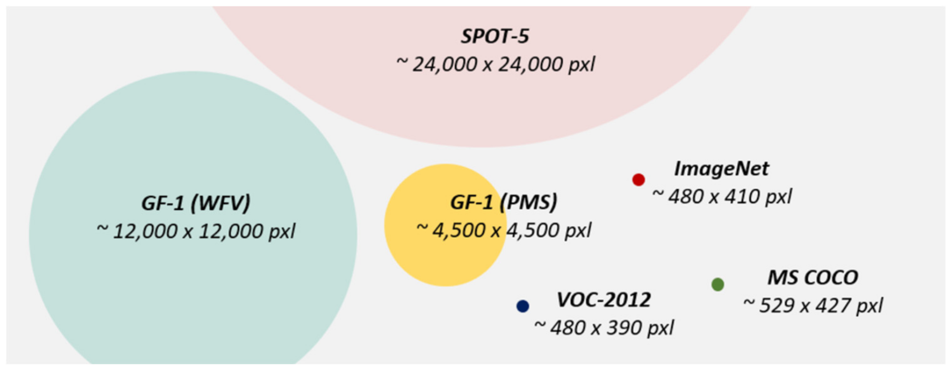
Remote sensing images are the ground information acquired by satellites, aircrafts, and unmanned aerial vehicles in the air. The image quality is susceptible to weather, light, moisture, and other natural factors in the imaging process. Owing to the high shooting position, the background information is more complex, and the imaging area is far more widespread than a natural image. For one image frame, a single-view remote sensing image covers area at least a few tens of square kilometers [47]. Therefore, the data volume of a remote sensing image is larger than that of a natural image [48]. Figure 1 illustrates a data volume comparison between a remote sensing image and a natural image. The above reasons increase the difficulty of satellite images object detection. In the past, the detection targets in remote sensing images were aircrafts and ships [49], which cover a large area. Song et al. detected airplanes and ships from a satellite image by extracting ROIs (airports and ports) containing potential objects which have a clear straight-line contour. This method avoids the problems of low efficiency and high false detection rate in detecting the whole image [50]. Nevertheless, this detection algorithm is only suitable for detecting hierarchical objects with evident geospatial features and cannot be applied to detect other targets, especially small ones. In remote sensing images, an oil well is much smaller than a plane or a ship, which increases the difficulty of detection. This paper proposes a solution to solve the problems of small-object detection in large-scale and high-resolution remote sensing images, which enables oil wells to be detected accurately. The main contributions of this article are as follows:

Figure 1.
Data volume comparison between a single-view remote sensing imagery and an average image size for VOC, ImageNet, and COCO [48].
- -
- Creation of an annotated dataset for oil well detection and follow-up research.
- -
- Investigation of a reliable model for oil well detection that can provide accurate and effective information of oil wells for governmental management.
- -
- Improvement of a state-of-the-art object detection algorithm to enable accurate small-object detection in large-scale and high-resolution satellite images.
2. Related Work
In this section, the related theories of the object detection algorithms used in this study are given first. Next, we introduce the used remote sensing image and the process of dataset marking. Lastly, the parameters of model training and the detection results of two models are provided.
2.1. SSD Network Framework
SSD (Single Shot Multibox Detector) is a typical one-stage target detection algorithm. Its network structure uses VGG16 as the basic framework (Figure 2). The main change is to transform fully connected layers of the sixth and the seventh layers into two convolutional layers. Four convolutional layers are then added after the seventh layer to output six feature maps of different sizes: 38 × 38, 19 × 19 for small-target detection, 10 × 10 and 5 × 5 for medium-target detection, and 3 × 3 and 1 × 1 for large-target detection. SSD regards the grids on the feature maps as the center and generates different aspect ratios anchor boxes according to the default mechanism. The number of anchor boxes generated in a single grid of each scale feature map is 4, 6, 6, 6, 4, and 4. Each anchor box is calculated confidence values of different classes and four coordinate values (x, y, w, h), which can be used to predict the class and location of targets to achieve the goal of classification on different scales.

Figure 2.
Layer architecture of the SSD network.
Loss function is also called cost function, which is used to evaluate the degree of deviation between predicted and real values of an algorithm. The smaller the loss value is, the better the algorithm performance is. In different algorithms, diverse loss functions are built to evaluate the algorithm performance. In SSD, the loss function is composed of class confidence and location losses. The formula is as follows:
where N is the number of default boxes; is the location loss, which adopts smooth L1 function:
Lonf(x, c) refers to the loss of class confidence, which adopts the softmax function:
where x is the matching results between the prediction and ground truth boxes of different classes; c and l are the class confidence value and location information of the prediction boxes, respectively; g is the location information of the ground truth boxes; P is the number of prediction classes; Pos stands for the positive sample; Neg stands for the negative sample; the weight term α is set to 1 by cross-validation.
2.2. YOLO v4 Network Framework
YOLO v4 (You Look Only Once) is a real-time, accurate, and easy-to-use regression algorithm developed from YOLO v3, which has a low false detection rate of the background. Compared with the previous YOLO models, YOLO v4 has three important improvements: adding a multiscale prediction function, better deep convolutional networks, and optimizing the classifier.
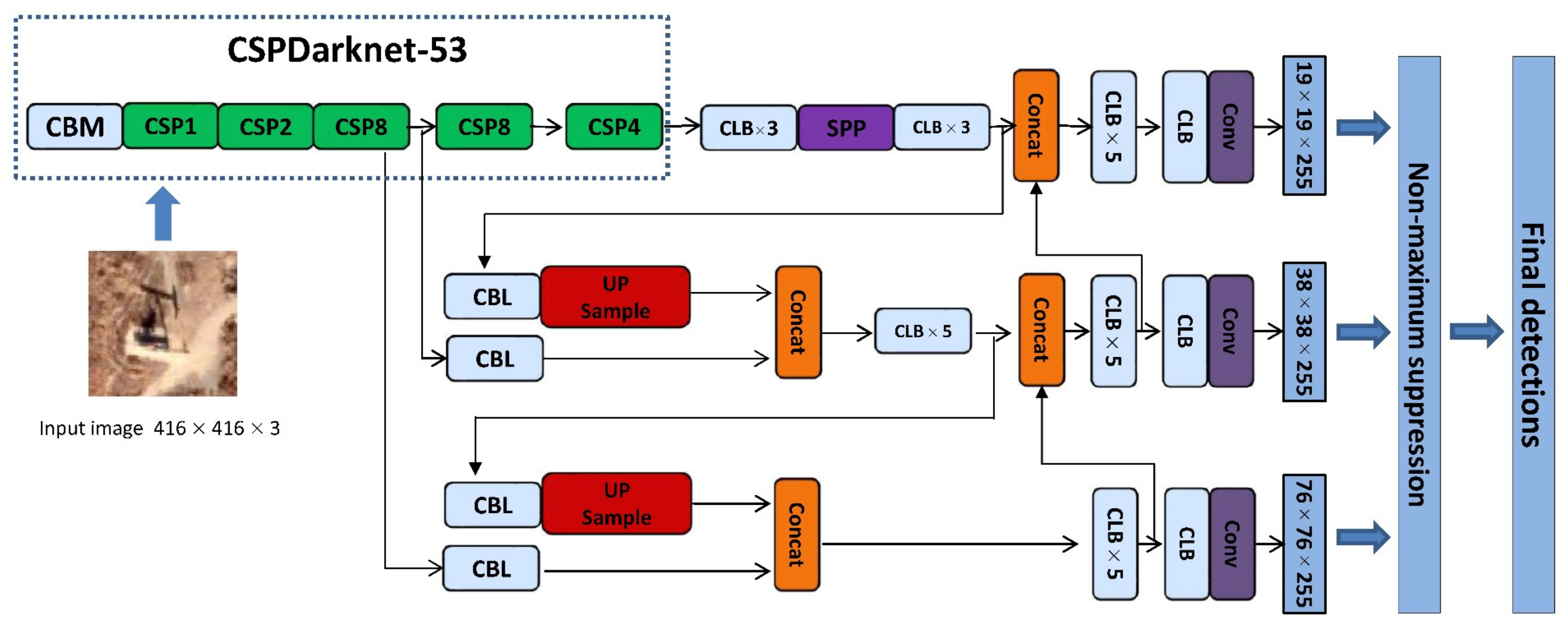
YOLO v4 extracts the target feature through CSPDarknet-53 and generates three feature maps with sizes of 76 × 76, 38 × 38, and 19 × 19, which are used to detect small, medium, and large targets, respectively. The feature map with the size of 19 × 19 is regarded as an example: the input image is split into 19 × 19 grids, and each cell is responsible for the detection of objects in its own area. During detection, the confidence value of each class and the coordinate information of anchor boxes in every grid are computed. The coordinates and the size of the prediction boxes are corrected by adding abscissa, ordinate, width, and height offsets to the corresponding anchor boxes. In YOLO v4, each grid generates three prediction boxes with confidence, coordinates, and size. The non-maximum suppression algorithm is used to filter out the prediction boxes with low confidence to obtain the final prediction result. A simplified layer structure of YOLO v4 is shown in Figure 3.
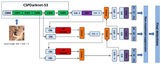
Figure 3.
Layer architecture of the YOLO v4 network.
In YOLO v4, the loss function is constructed of three parts: class, location, and confidence losses. In this study, only a single class was detected, hence, the class loss needed not be calculated.
The location loss is:
The confidence loss is:
where indicates whether the jth anchor box in the ith grid includes the current target. If so, then it is 1, otherwise it is 0. B is the number of anchor boxes in each grid; represent the center coordinates and the width and height of the anchor boxes, and , are the corresponding manually marked values; indicates that when the jth anchor box in the ith grid does not include the current target, the value is 1; otherwise, it is 0; is the weight coefficient.
2.3. Dataset
The study area is located in Daqing City of Heilongjiang Province, Northeast China. Daqing Oilfield, the largest continental sandstone oilfield in China, is an important oil production base [51]. The detection type of the oil well in this study is beam-pumping well, which is a ubiquitous equipment in the Daqing Oilfield in accordance with the field survey. The advantages of a beam-pumping well are as follows: (1) strong applicability, reliable operation, and low environmental requirements, which can be used from the north to the south of China; (2) simple structure, convenient maintenance, and long service life. For the above characteristics, it is the most used oil exploration facility in the Daqing Oilfield. Figure 4 shows the types of oil wells recorded in the field survey.

Figure 4.
Oil wells in the field survey: (a) a single beam-pumping well; (b) a cluster of beam-pumping wells; (c) an inoperative belt-pumping well.
In this study, Saertu District of Daqing City was selected as the training area, and a part of Ranghulu District of Daqing City was selected as the test area (Figure 5). The oil wells in the selected areas are densely distributed, which is helpful to analyze the training and detection results. In deep learning, the dataset plays an important role for the final results. A comprehensive and accurate dataset can effectively elevate the generalization capability and robustness of a deep learning algorithm.
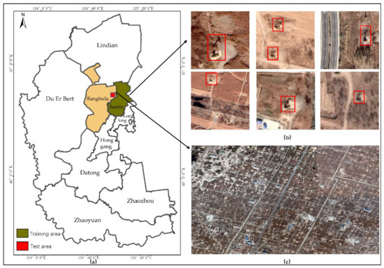
Figure 5.
Study area: (a) location of Daqing City; (b) clear image blocks of the oil well in the training area; (c) part of remote sensing image of the test area.
At present, the known public datasets do not contain oil wells, such that public datasets cannot support our study. For this reason, we used Google Earth images with the spatial resolution of 0.26 m to make our own dataset. Google Earth images are multiple data source images which integrate various remote sensing data, mainly including two categories: satellite and aerial data. Google Earth images have the advantages of wide coverage, multilevel products, and high resolution. To obtain high-quality training data as much as possible, we operated as follows (Figure 6):

Figure 6.
Process of marking oil well labels.
- -
- The remote sensing image that was cloudless, clear and had minimal time difference was screened for mosaicking.
- -
- A mosaic image was cut into several blocks coincident with the input size of model training by using a cutting tool, and clear image blocks of oil wells were selected.
- -
- Data augmentation. Mirroring, noise, and fuzziness were applied to the image blocks to expand the oil well dataset and elevate the generalization capability of the model.
- -
- The labels of oil wells were elaborated; the format is the same as in the Pascal VOC dataset. Finally, an oil well dataset with 5895 images was obtained (https://github.com/Stevenshi1002/oil-well-dataset, 3 August 2021).
2.4. Experiment and Evaluation
We conducted all the experiments on the same computer to test the detection capability of two deep learning algorithms fairly. The hardware platform was Intel(R) Core(TM) i7-8700K CPU at 3.70 GHz, NVIDIA GTX 1070 GPU, and the running memory was 16 GB. In this study, all of our algorithms were coded using Python 3.7.4 and the Keras high-level API for neural networks.
A total of 5895 images exist in the oil well dataset, and each image contains 1–5 oil wells. The dataset was randomly divided into three parts: 480 images of the dataset as the test set, 540 images as the validation set, and 4875 images as the training set. Traditional deep learning model training requires sufficient data, long time, and high-performance computing hardware. The emergence of transfer learning breaks this limitation. Given a certain relationship between the source domain and the target, the knowledge extracted from the source domain can be used in training the target detection model. This approach transforms the deep learning algorithm from traditional scratch learning into cumulative learning, which not only reduces the cost of model training but also significantly improves the effect of a deep learning algorithm. Thus, in this paper, we introduced parameters pretrained on the Pascal VOC dataset to initialize the weights of SSD and YOLO v4. Furthermore, our own oil well dataset was used to fine-tune parameters to improve model performance.
In this study, the training continued through 60 epochs and was divided into two stages, with 30 rounds in the first stage and the second stage, respectively. In the first stage, the batch size was defined as 16, and the initial value of the learning rate was 0.0001. In the second stage, the batch size was defined as 8, and the learning rate dropped to 0.00001. In the training process, we adopted early stopping to avoid overfitting. The training of SSD and YOLO v4 took about 10.5 h and 9 h, when the validation loss reached a plateau.
In the evaluation of model performance, two indexes are widely used, which include precision and recall. However, when the precision is high, the recall cannot be guaranteed to be as high as the precision. Similarly, considering the recall alone cannot objectively assess the detection capability of the model. In this study, the precision–recall curve (PRC) was adopted as the evaluation index for two object detection models, which is composed of precision (P) and recall (R). Precision is the proportion of real oil wells in the detected oil wells. Recall is the proportion of correctly detected oil wells in the actual number of oil wells in the image. The precision and recall indicators are calculated using Formulas (6) and (7). The confusion matrix of oil well detection is shown in Table 1.

Table 1.
Confusion matrix of oil well detection.
PRC is the area of the precision–recall curve. The higher the PRC value is, the stronger the detection capability of the model is [52]. As shown in Figure 7, the PRC of YOLO v4 (94.7%) was higher than that of SSD (93.2%) in oil well detection.
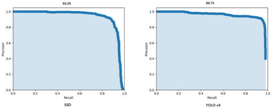
Figure 7.
PRC for SSD and YOLO v4.
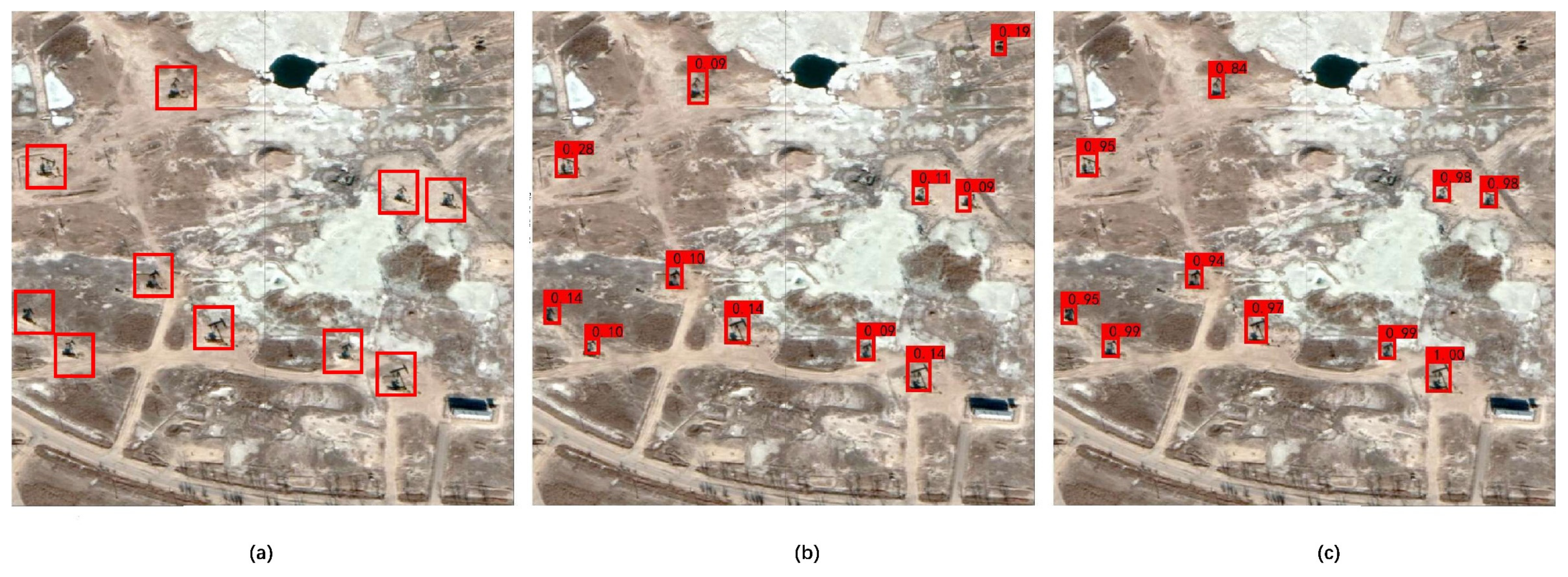
For further comparing the performance of two models in this study, we tested a small-scale remote sensing image by using trained models. Using this method, the detection capability of SSD and YOLO v4 can be evaluated directly with visual results. The ground truth image (Figure 8a) and its corresponding detection results obtained by SSD (Figure 8b) and YOLO v4 (Figure 8c) are presented in Figure 8. Ten oil wells exist in the test area; SSD detected eleven oil wells, with 10 real oil wells all accurately detected and 1 false detection, with the minimum confidence of 0.09 and the maximum of 0.28; YOLO v4 accurately detected all ten real oil wells, with the minimum confidence of 0.84 and the maximum of 1.0. The detection duration of SSD and YOLO v4 was about 9.45 s and 3.30 s, respectively. For the same oil well, the efficiency and confidence value of YOLO v4 were much higher than those of SSD, which illustrates that the oil well detection capability of YOLO v4 was better than that of SSD. Analysis of the network structure shows that YOLO v4 successfully used CSPDarknet-53 for feature extraction, which can regard the superimposed feature maps as a new input to the next layer by using its residual structure. It can also reduce the risk of gradient explosion when the network layer number increases and strengthen the network learning capability at the same time. It is conducive to extracting abundant small features of objects, and accordingly has great advantages in detecting small objects, such as oil wells. Therefore, YOLO v4 has better performance in oil well detection.
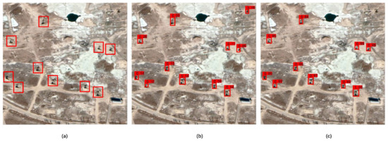
Figure 8.
Visual oil well detection results for SSD and YOLO v4. (a) the ground truth image; (b,c) the detection results obtained by SSD and YOLO v4.
3. Improvement of YOLO v4
In traditional deep learning object detection algorithms on satellite images, trained models are used to detect objects in small-scale satellite images such as Figure 8a or to detect objects from the captured satellite images (mostly in the JPG format). However, these images are not real remote sensing images because remote sensing has the important characteristic of wide-range coverage area. A single-view satellite image covers at least a few tens of square kilometers. Therefore, object detection in large-scale remote sensing images is more meaningful than that in small-scale ones. Furthermore, the object detection methods for small-scale remote sensing images cannot be applied to large-scale ones because the data volume of the former is much smaller than that of the latter. For the above reason, it is still difficult to detect targets directly in large-scale remote sensing images, especially small targets. To address this issue, YOLO v4 was improved in this study so that it could be used for oil well detection in a large-scale and high-resolution sensing image, which provides a feasible solution for small-object detection in large-scale remote sensing images.
3.1. Sliding Slices and Discarding Edges
In YOLO v4, the input image is divided into three scales of 19 × 19, 38 × 38, and 76 × 76 for object detection. The scale of 76 × 76 is for small-object detection, which is evidently adequate for a natural image. However, for large-scale remote sensing images, errors will occur in object detection. In terms of a satellite image with 30,000 × 30,000 pixels and the spatial resolution of 0.26 m, its coverage area is approximately 60 km2. When the 76 × 76 scale is used for object detection in such an image, the area of each grid is 395 × 395 pixels, which is much larger than the average size of oil wells (an oil well occupies approximately 500 pixels in a satellite image with the spatial resolution of 0.26 m). The targets that cannot be detected will appear in this condition.
In the beginning, we adopted the method of recognizing a large-scale remote sensing image in slices to detect small targets. That is, the input large-scale satellite image was cut into several image slices of 416 × 416 pixels, consistent with the size of the training data. The method detects each slice separately and then merges the results after detection to improve the oil well detection capability of YOLO v4 (Figure 9).
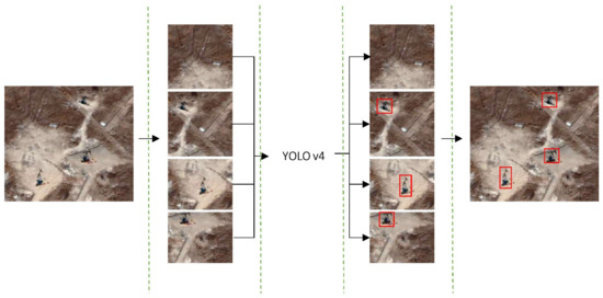
Figure 9.
Flowchart of detecting remote sensing images in slices.
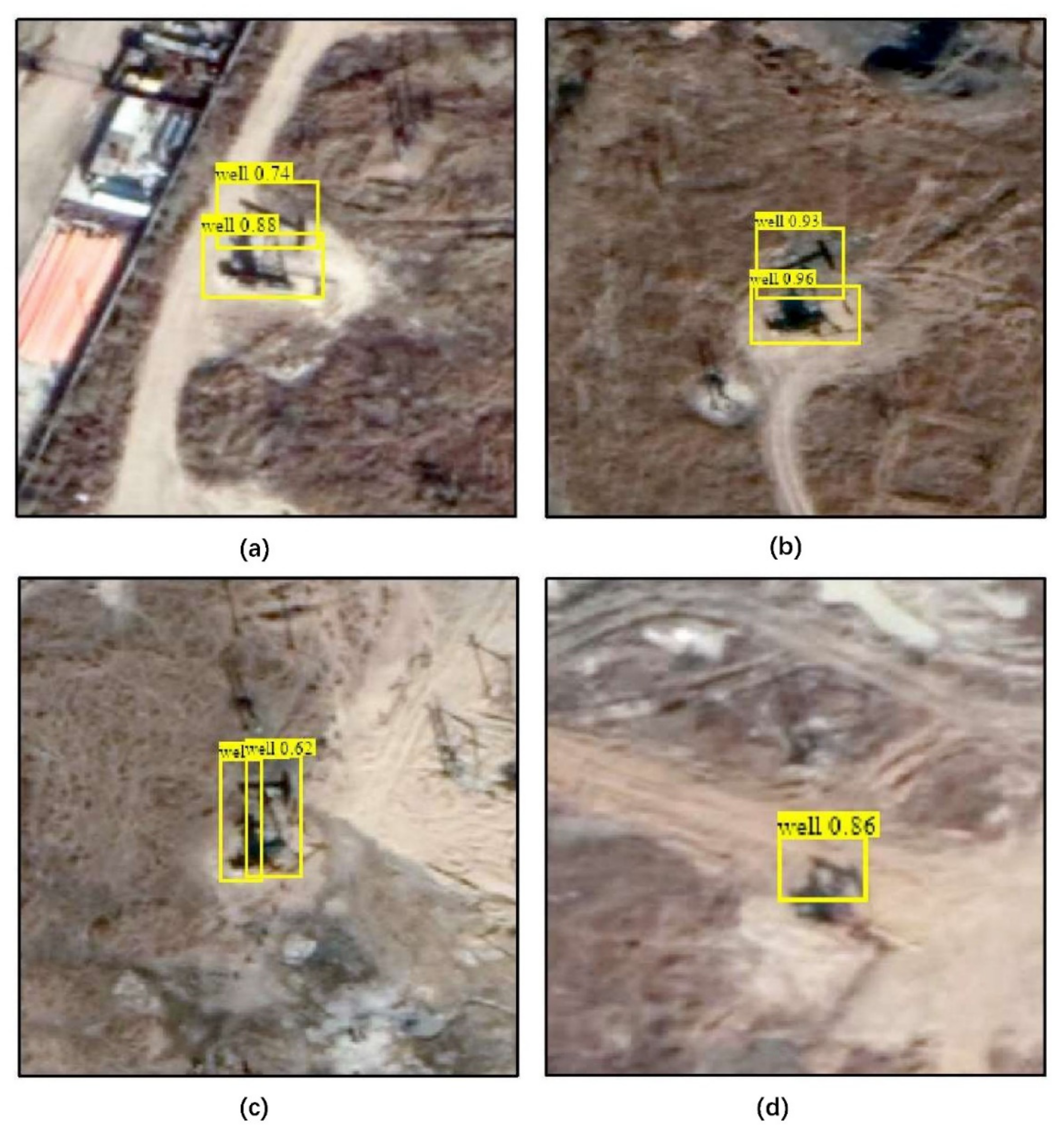
Although the slicing method can effectively increase the small-object detection capability of YOLO v4, it causes new problems for oil well detection. When a large-scale and high-resolution image is sliced, the oil wells on the tangent lines are segmented into different slices, which leads to the model being unable to detect them correctly due to partial deletion or detecting the same oil well in adjacent slices at the same time. The above shortcomings of this method cause repeated detection and inaccurate positioning, which reduce the detection accuracy rate (Figure 10).

Figure 10.
Oil wells on tangent lines are segmented into different slices, which causes repeated detection (a–c) and inaccurate positioning (d).
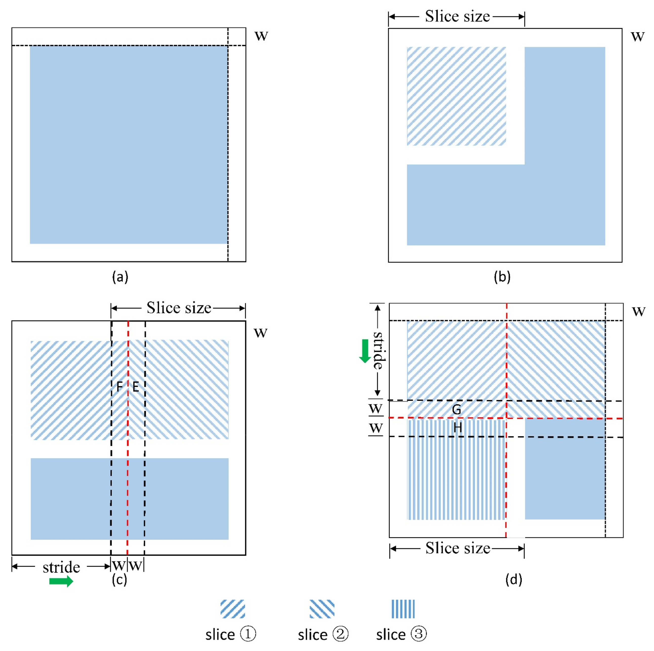
In view of the above drawbacks, we improved YOLO v4 with sliding slices and discarding edges to avoid the problems of repeated detection and inaccurate positioning during detection. The improved method detects a large-scale satellite image by using a sliding window and then discards the detection results within a certain width range around each slice. The improved method contains six steps, and the schematic is shown in Figure 11.

Figure 11.
Schematic of sliding slices and discarding edges. (a) the original image; (b,c,d) the detection process of slice ①, ② and ③.
Step 1: Define the slice size (the slice size in this study was 416 × 416 pixels) and the size of discarding edges (W, the discarding edges in this study were 60 pixels).
Step 2: Fill the image periphery by using a zero pixel value with the width W to prevent the oil wells in the outermost edge of the image from being discarded to affect detection results. Then, initialize the sliding window position.
Step 3: Detect oil wells in the valid area of the sliding window (valid size is the actual effective detection length of a single slice, valid size = slice size − 2W).
Step 4: Slide the window to the right with the defined stride to detect oil wells until it reaches the right boundary of the remote sensing image (a stride is the sliding size of the sliding window, stride = slice size − 2W).
Step 5: Slide the window back to the leftmost position and add a stride down.
Step 6: Repeat steps 3–5 until sliding to the lower right edge of the image.
The discarding edges (W) are determined by the maximum value of anchor boxes acquired using the k-means algorithm to ensure that the oil wells on tangent lines can be effectively detected only once. Anchor boxes first come from Faster R-CNN, a group of initial candidate boxes with the width and height fixed in advance to boost the accuracy and convergence speed in model training [17]. In Faster R-CNN, the size of anchor boxes is defined manually. In YOLO v4, the k-means algorithm is applied to cluster the training dataset to determine the average sizes of the anchor boxes. YOLO v4 divides an image into three scales. Every grid in each scale generates three anchor boxes, such that a total of nine different sizes of anchor boxes are considered in this study (Table 2). When the discarding edges and the sliding stride are defined and the algorithm is executed, every two adjacent slices have overlapping and discarding areas. For example, in Figure 11, when slice ① is in the process of oil well detection, its overlapping areas with slices ② and ③ are E, F and G, H, discarding areas are E and H; when slices ② and ③ are in the process of oil well detection, their discarding areas with slice ① are F and G, respectively. Then, even if some oil wells on tangent lines are cut into different slices, the discarding edges regard them as invalid detection. Consequently, the final detection results remain unaffected.

Table 2.
Different sizes of anchor boxes in this study.
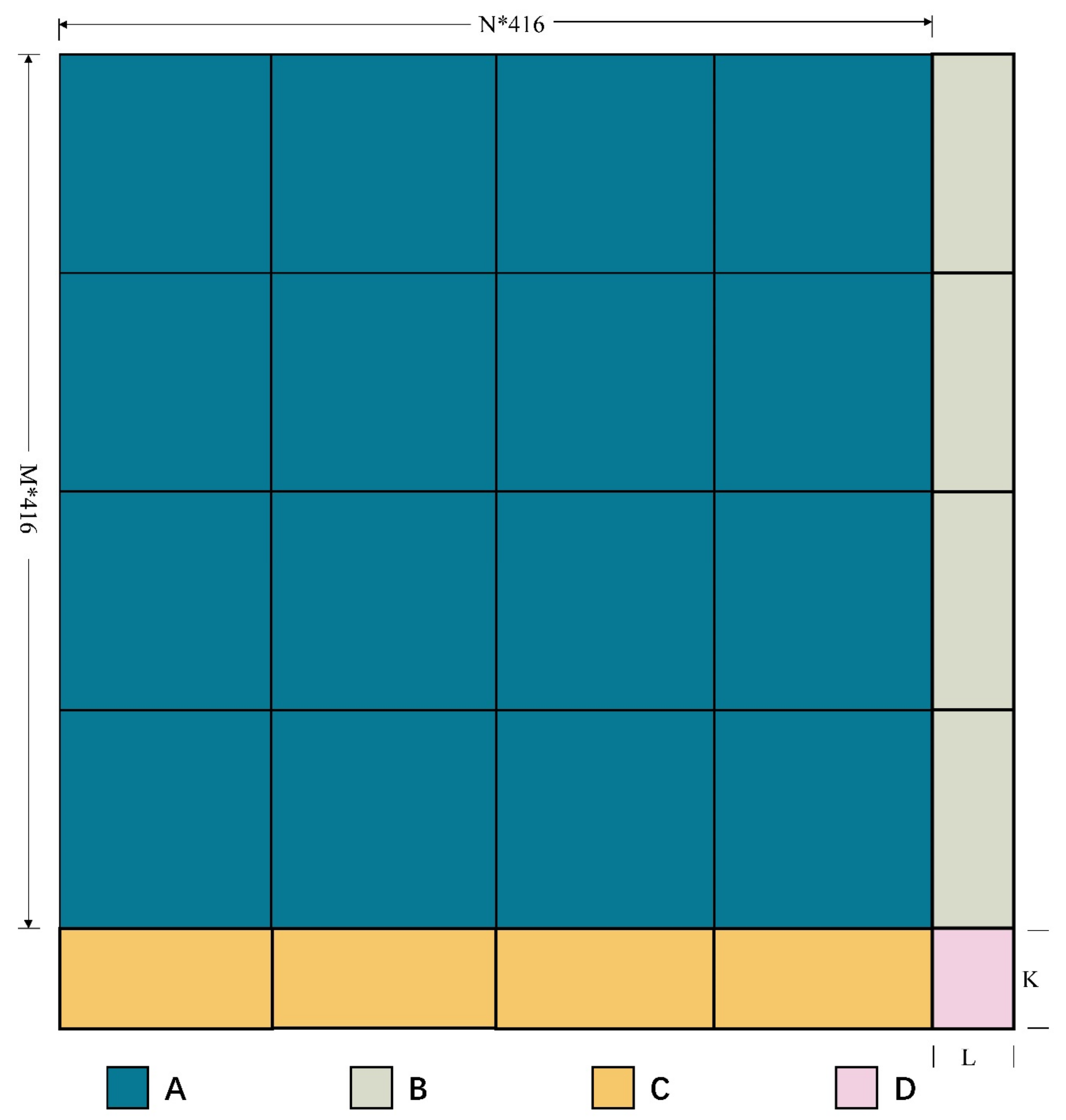
In the detection process, for a large-scale image of any size, when the sliding window is in different positions, the slice size should also be adjusted. In this study, four types of slice sizes are considered. In Figure 12, the size of area A is m × n × 416 × 416 pixels, which can be completely sliced using an initialized sliding window; in area B, L < 416 pixels, which can only be completely sliced in the vertical direction; in area C, K < 416, which can only be completely sliced in the horizontal direction; area D is a single slice with the size of K × L pixels. When the sliding window is located in four different areas, the slice size is dynamically adjusted to ensure accurate motion detection.
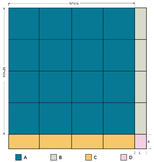
Figure 12.
Four types of slice sizes in this study.
3.2. Vectorization of Detection Results
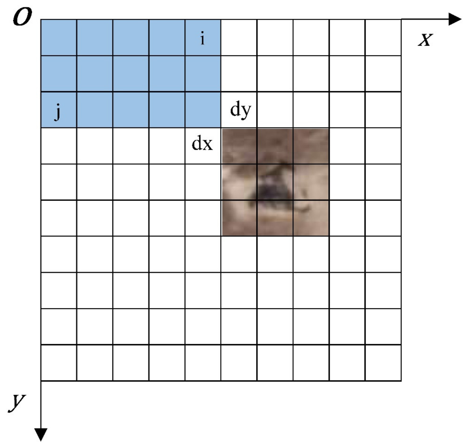
The locations of oil wells detected using the improved YOLO v4 are the pixel coordinates on the satellite image; however, they have no geographical information. The final result also cannot show the distribution of oil wells on the geographical level. Therefore, pixel coordinates should be converted into geographic coordinates of the final result. The coordinate system of a remote sensing image is shown in Figure 13.

Figure 13.
Coordinate system of a remote sensing image.
The conversion formula for pixel and geographical coordinates is as follows:
where Xgeo and Ygeo represent the geographical coordinates in the remote sensing image; i and j are the column and row numbers of the image pixel, respectively; X0 and Y0 are the geographical coordinates of the origin in the remote sensing image; dx and dy are the horizontal and vertical resolutions of the image, respectively. GT(0) and GT(1) denote the image rotation coefficients. We obtained the affine matrix of remote sensing images through the Geospatial Data Abstraction Library (GDAL). The affine matrix contained the geographic coordinates of the origin, the horizontal and vertical resolutions, and the rotation coefficients of the satellite image. Therefore, the geographic coordinates of oil wells detected can be calculated through Formula (8).
3.3. Results
In this study, the image size of the study area was 34,044 × 29,693 pixels, which is approximately 68.33 km2. The image was input into the YOLO v4 model trained with our oil well dataset; however, the model could not detect oil wells with the whole remote sensing image because of its limited detection capability for large-scale remote sensing images. Through the improvement with sliding slices and discarding edges of YOLO v4, the model is suitable for oil well detection in large-scale satellite images. In the detection process, the slice size was set to 416 × 416, and the score and IOU threshold were set to 0.45 and 0.5, respectively.
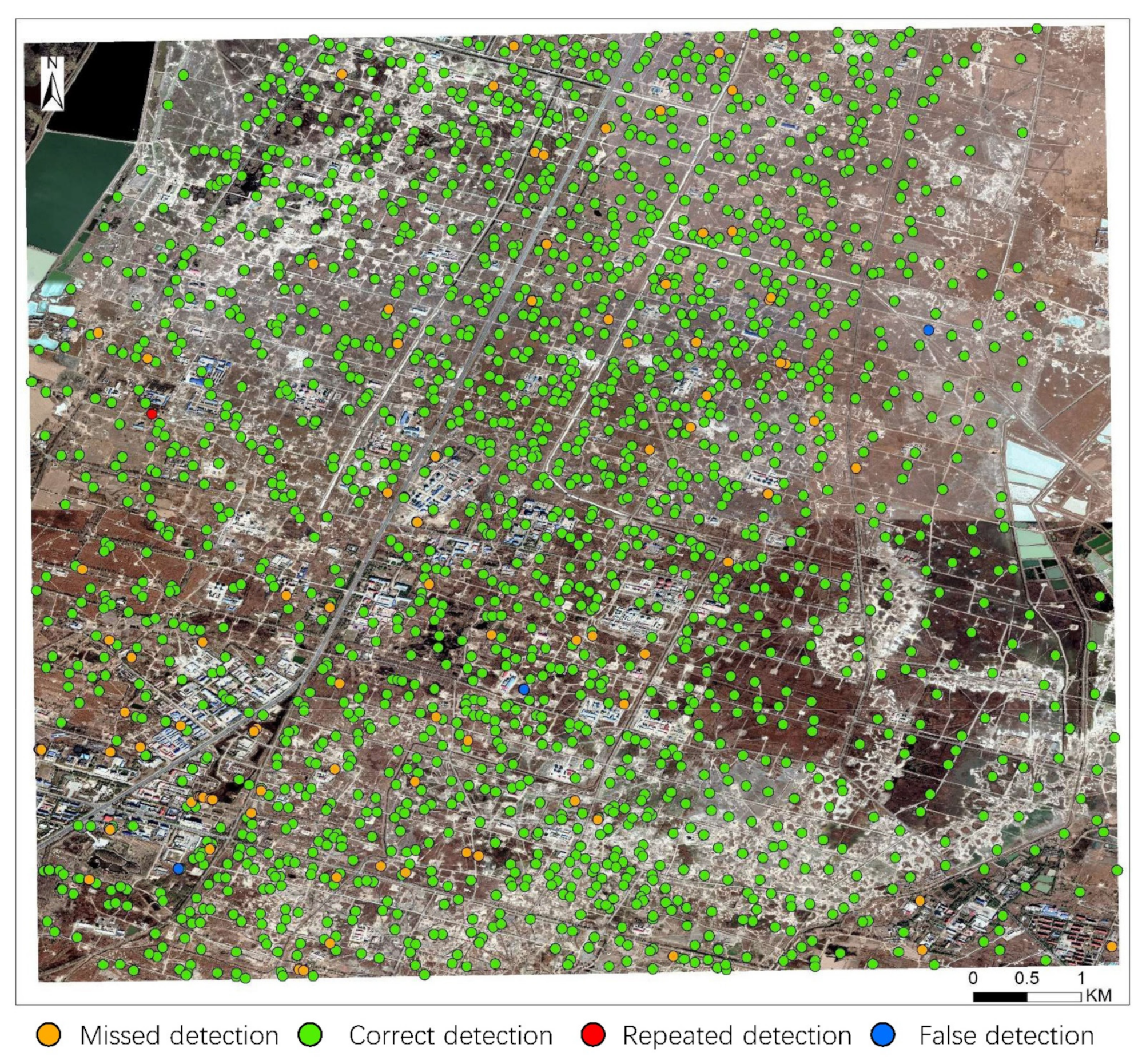
In accordance with the results of manual interpretation and field validation, 2023 oil wells exist in the study area. When the discarding edges were unset and only the slice operation was performed, a total of 2052 oil wells were detected, with 152 cases of repeated detection and inaccurate positioning, 16 cases of false detection, and 139 cases of missed detection. The detection results are shown in Figure 14. When the algorithm is executed, it divides a large number of oil wells on tangent lines into different slices, causing noticeable repeated detection. Then, the discarding edges were set to 60 pixels, which is slightly larger than the maximum size of an oil well. The other parameters remained unchanged, and the detection results are shown in Figure 15. After the discarding edges were set, a total of 1937 oil wells were detected, with one case of repeated detection and inaccurate positioning, three cases of false detection, and 90 cases of missed detection. When the slice size and discarding edges were set, the oil well detection precision and recall of the improved model were 99.8% and 95.6%, respectively. Compared with Figure 14 and Figure 15 indicates that the discarding edges can effectively resolve the problem of repeated detection and inaccurate positioning under the same conditions and greatly heighten the detection accuracy of the model.
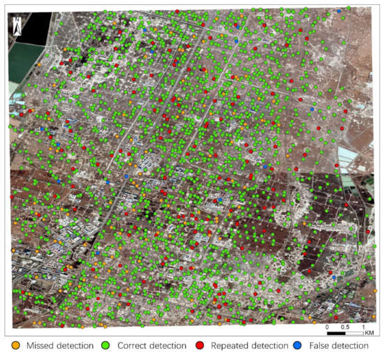
Figure 14.
Detection result with unset discarding edges.
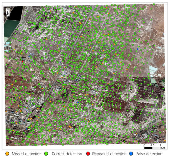
Figure 15.
Detection result with the discarding edges set to 60.
However, the two experimental results indicate that the model still had the phenomenon of missed detection, which was caused by the following reasons: (1) a few of the oil wells were not beam-pumping wells but belt-pumping wells or other types of oil wells, which could not be detected by the current model; (2) the direction of oil well construction made the detection of some oil wells difficult. When an oil well is constructed in the east–west direction, it presents a T-like shape in the satellite image, occupies substantial pixels, and has strong features; it is easy to detect using a trained model. On the contrary, when the oil well is constructed in the north–south direction, it presents an I-like shape, occupies fewer pixels, presents unobvious features, and is easily confused with poles and mobile phone base stations, which makes them difficult to be detected (Figure 16).

Figure 16.
Oil wells constructed in the north–south direction.
4. Conclusions
In this study, the two most commonly used deep learning algorithms in objection detection, YOLO v4 and SSD, were compared in terms of oil well detection. Owing the lack of a corresponding public dataset, we made our own oil well dataset to support experiments. The two algorithms showed good capability in oil well detection, but the performance of YOLO v4 was better. At present, in the field of remote sensing image object detection, most of the detection data are JPG format images of small areas captured from large-scale satellite images, and the targets are large objects, such as aircrafts and ships. This limitation is due to the difficulty of detecting small objects in large-scale remote sensing images. To address this problem, we improved YOLO v4 with sliding slices and discarding edges. Comparative and confirmatory tests indicate that the sliding slices and discarding edges can effectively resolve the repeated detection and inaccurate positioning and accurately detect oil wells in a large-scale and high-resolution satellite image, which provides a new idea for small-object detection in large-scale and high-resolution remote sensing images. The number of oil wells accurately detected adopting this method can provide reliable basic data for governments and contribute to policymaking.
The study area was limited to the Daqing Oilfield, and the detection type of oil wells was beam-pumping well, which was limited by the dataset used for training. In the future, additional types images of oil wells should be collected to enhance the dataset. At the same time, the satellite image used for training and detection in this study has only three bands of R, G, B. If other spectral information is added in the research, the detection accuracy may be improved. Thus, the application of multispectral and hyperspectral images is the focus of future research. The exploitation of oil affects the environment in different aspects, such as land use change, soil pollution, vegetation damage, and water pollution. Therefore, the detection of oil wells is also valuable in these aspects.
Author Contributions
P.S. and C.S. developed the original idea for the study and completed the manuscript. Q.J. revised the paper. B.L., Z.Z., Q.W., G.T., S.Z., J.X. and X.G. contributed to data collection. C.S. helped complete program code. All authors have read and agreed to the published version of the manuscript.
Funding
This research was funded by the geological survey project of China Geological Survey (DD 20190705).
Data Availability Statement
The oil well dataset has been uploaded to: https://github.com/Stevenshi1002/oil-well-dataset.
Acknowledgments
Satellite images used in this article were provided by the Google Earth platform. We are grateful to them for allowing us to use their data.
Conflicts of Interest
The authors declare no conflict of interest.
References
- Zou, C.N.; Yang, Z.; Sun, S.S.; Zhao, Q.; Bai, W.H.; Liu, H.L.; Pan, S.Q.; Wu, S.T.; Yuan, Y.L. Exploring petroleum inside source kitchen: Shale oil and gas in Sichuan Basin. Sci. China-Earth Sci. 2020, 63, 934–953. [Google Scholar] [CrossRef]
- Guo, K.; Li, H.L.; Yu, Z.X. In-situ heavy and extra-heavy oil recovery: A review. Fuel 2016, 185, 886–902. [Google Scholar] [CrossRef]
- Campbell, C.J. The assessment and importance of oil depletion. Energy Explor. Exploit. 2002, 20, 407–435. [Google Scholar] [CrossRef]
- Ma, Z.; Chen, S.; Shuai, S.; Xie, F.; Xie, C. Application of Remote Sensing Technology in Investigation of Oil and gas Development Status. China Resour. Compr. Util. 2020, 38, 47–48. [Google Scholar]
- Ozturk, T.; Talo, M.; Yildirim, E.A.; Baloglu, U.B.; Yildirim, O.; Acharya, U.R. Automated detection of COVID-19 cases using deep neural networks with X-ray images. Comput. Biol. Med. 2020, 121, 103792. [Google Scholar] [CrossRef]
- Weiss, M.; Jacob, F.; Duveiller, G. Remote sensing for agricultural applications: A meta-review. Remote Sens. Environ. 2020, 236. [Google Scholar] [CrossRef]
- Dasgupta, B.; Gupta, A.; Ray, A. Dark matter capture in celestial objects: Light mediators, self-interactions, and complementarity with direct detection. J. Cosmol. Astropart. Phys. 2020, 10. [Google Scholar] [CrossRef]
- Lei, Y.G.; Yang, B.; Jiang, X.W.; Jia, F.; Li, N.P.; Nandi, A.K. Applications of machine learning to machine fault diagnosis: A review and roadmap. Mech. Syst. Signal Proc. 2020, 138, 39. [Google Scholar] [CrossRef]
- Ma, L.; Liu, Y.; Zhang, X.L.; Ye, Y.X.; Yin, G.F.; Johnson, B.A. Deep learning in remote sensing applications: A meta-analysis and review. ISPRS-J. Photogramm. Remote Sens. 2019, 152, 166–177. [Google Scholar] [CrossRef]
- Viola, P.; Jones, M.J. Robust real-time face detection. Int. J. Comput. Vis. 2004, 57, 137–154. [Google Scholar] [CrossRef]
- Dalal, N.; Triggs, B. Histograms of oriented gradients for human detection. In Proceedings of the 2005 IEEE Computer Society Conference on Computer Vision and Pattern Recognition, San Diego, CA, USA, 20–25 June 2005; Schmid, C., Soatto, S., Tomasi, C., Eds.; IEEE Computer Soc: Los Alamitos, CA, USA, 2005; pp. 886–893. [Google Scholar]
- Forsyth, D. Object Detection with Discriminatively Trained Part-Based Models. Computer 2014, 47, 6–7. [Google Scholar] [CrossRef]
- Krizhevsky, A.; Sutskever, I.; Hinton, G.E. ImageNet Classification with Deep Convolutional Neural Networks. Commun. ACM 2017, 60, 84–90. [Google Scholar] [CrossRef]
- Li, M.; Zhang, Z.; Lei, L.; Wang, X.; Guo, X. Agricultural Greenhouses Detection in High-Resolution Satellite Images Based on Convolutional Neural Networks: Comparison of Faster R-CNN, YOLO v3 and SSD. Sensors 2020, 20, 4938. [Google Scholar] [CrossRef] [PubMed]
- Carranza-Garcia, M.; Torres-Mateo, J.; Lara-Benitez, P.; Garcia-Gutierrez, J. On the Performance of One-Stage and Two-Stage Object Detectors in Autonomous Vehicles Using Camera Data. Remote Sens. 2021, 13, 89. [Google Scholar] [CrossRef]
- Li, J.N.; Liang, X.D.; Shen, S.M.; Xu, T.F.; Feng, J.S.; Yan, S.C. Scale-Aware Fast R-CNN for Pedestrian Detection. IEEE Trans. Multimed. 2018, 20, 985–996. [Google Scholar] [CrossRef] [Green Version]
- Ren, S.; He, K.; Girshick, R.; Sun, J. Faster r-cnn: Towards real-time object detection with region proposal networks. arXiv 2015, arXiv:1506.01497. [Google Scholar] [CrossRef] [PubMed] [Green Version]
- He, K.M.; Gkioxari, G.; Dollar, P.; Girshick, R. Mask R-CNN. IEEE Trans. Pattern Anal. Mach. Intell. 2020, 42, 386–397. [Google Scholar] [CrossRef]
- Wang, J.L.; Luo, J.X.; Liu, B.; Feng, R.; Lu, L.N.; Zou, H.D. Automated diabetic retinopathy grading and lesion detection based on the modified R-FCN object-detection algorithm. IET Comput. Vis. 2020, 14, 1–8. [Google Scholar] [CrossRef]
- Zhang, J.M.; Xie, Z.P.; Sun, J.; Zou, X.; Wang, J. A Cascaded R-CNN With Multiscale Attention and Imbalanced Samples for Traffic Sign Detection. IEEE Access 2020, 8, 29742–29754. [Google Scholar] [CrossRef]
- Liu, W.; Anguelov, D.; Erhan, D.; Szegedy, C.; Reed, S.; Fu, C.Y.; Berg, A.C. SSD: Single Shot MultiBox Detector. In Proceedings of the Computer Vision—ECCV 2016, Amsterdam, The Netherlands, 11–14 October 2016; Leibe, B., Matas, J., Sebe, N., Welling, M., Eds.; Springer International Publishing: Cham, Switzerland, 2016; Volume 9905, pp. 21–37. [Google Scholar]
- Bochkovskiy, A.; Wang, C.-Y.; Liao, H.-Y.M. Yolov4: Optimal speed and accuracy of object detection. arXiv 2020, arXiv:2004.10934. [Google Scholar]
- Liu, Z.; Shen, C.; Fan, X.; Zeng, G.; Zhao, X. Scale-aware limited deformable convolutional neural networks for traffic sign detection and classification. IET Intell. Transp. Syst. 2020, 14, 1712–1722. [Google Scholar] [CrossRef]
- Hu, X.W.; Xu, X.M.; Xiao, Y.J.; Chen, H.; He, S.F.; Qin, J.; Heng, P.A. SINet: A Scale-Insensitive Convolutional Neural Network for Fast Vehicle Detection. IEEE Trans. Intell. Transp. Syst. 2019, 20, 1010–1019. [Google Scholar] [CrossRef] [Green Version]
- Li, G.F.; Yang, Y.F.; Qu, X.D. Deep Learning Approaches on Pedestrian Detection in Hazy Weather. IEEE Trans. Ind. Electron. 2020, 67, 8889–8899. [Google Scholar] [CrossRef]
- Jin, X.L.; Tang, R.C.; Liu, L.F.; Wu, J.G. Vehicle license plate recognition for fog-haze environments. IET Image Process. 2021, 15, 1273–1284. [Google Scholar] [CrossRef]
- Morera, A.; Sanchez, A.; Moreno, A.B.; Sappa, A.D.; Velez, J.F. SSD vs. YOLO for Detection of Outdoor Urban Advertising Panels under Multiple Variabilities. Sensors 2020, 20, 4587. [Google Scholar] [CrossRef] [PubMed]
- Dian, R.; Li, S.; Guo, A.; Fang, L. Deep Hyperspectral Image Sharpening. IEEE Trans. Neural Netw. Learn. Syst. 2018, 29, 5345–5355. [Google Scholar] [CrossRef]
- Zampieri, A.; Charpiat, G.; Girard, N.; Tarabalka, Y. Multimodal Image Alignment Through a Multiscale Chain of Neural Networks with Application to Remote Sensing. In Proceedings of the Computer Vision—ECCV 2018, Munich, Germany, 8–14 September 2018; Volume 11220, pp. 679–696. [Google Scholar]
- Cheng, G.; Yang, C.; Yao, X.; Guo, L.; Han, J. When Deep Learning Meets Metric Learning: Remote Sensing Image Scene Classification via Learning Discriminative CNNs. IEEE Trans. Geosci. Remote Sens. 2018, 56, 2811–2821. [Google Scholar] [CrossRef]
- Carranza-Garcia, M.; Garcia-Gutierrez, J.; Riquelme, J.C. A Framework for Evaluating Land Use and Land Cover Classification Using Convolutional Neural Networks. Remote Sens. 2019, 11, 274. [Google Scholar] [CrossRef] [Green Version]
- Guo, S.C.; Jin, Q.Z.; Wang, H.Z.; Wang, X.Z.; Wang, Y.G.; Xiang, S.M. Learnable Gated Convolutional Neural Network for Semantic Segmentation in Remote-Sensing Images. Remote Sens. 2019, 11, 1922. [Google Scholar] [CrossRef] [Green Version]
- Das, M.; Ghosh, S.K. Deep-STEP: A Deep Learning Approach for Spatiotemporal Prediction of Remote Sensing Data. IEEE Geosci. Remote Sens. Lett. 2016, 13, 1984–1988. [Google Scholar] [CrossRef]
- Cai, Y.; Guan, K.; Peng, J.; Wang, S.; Seifert, C.; Wardlow, B.; Li, Z. A high-performance and in-season classification system of field-level crop types using time-series Landsat data and a machine learning approach. Remote Sens. Environ. 2018, 210, 35–47. [Google Scholar] [CrossRef]
- Yang, F.; Li, W.; Li, W.; Wang, P. (SOD)-O-3: Single Stage Small Object Detector from Scratch for Remote Sensing Images. In Proceedings of the Image and Graphics, ICIG 2019, Beijing, China, 23–25 August 2019; Volume 11903, pp. 347–358. [Google Scholar] [CrossRef]
- Ren, Y.; Zhu, C.; Xiao, S. Small Object Detection in Optical Remote Sensing Images via Modified Faster R-CNN. Appl. Sci. 2018, 8, 813. [Google Scholar] [CrossRef] [Green Version]
- Chen, X.; Kundu, K.; Zhu, Y.; Ma, H.; Fidler, S.; Urtasun, R. 3D Object Proposals Using Stereo Imagery for Accurate Object Class Detection. IEEE Trans. Pattern Anal. Mach. Intell. 2018, 40, 1259–1272. [Google Scholar] [CrossRef] [Green Version]
- Han, Y.; Han, Y. A Deep Lightweight Convolutional Neural Network Method for Real-Time Small Object Detection in Optical Remote Sensing Images. Sens. Imag. 2021, 22, 24. [Google Scholar]
- Zhang, W.; Wang, S.; Thachan, S.; Chen, J.; Qian, Y. Deconv R-CNN for small object detection on remote sensing images. In Proceedings of the IGARSS 2018—2018 IEEE International Geoscience and Remote Sensing Symposium, Valencia, Spain, 22–27 July 2018; pp. 2483–2486. [Google Scholar]
- Lin, T.-Y.; Maire, M.; Belongie, S.; Hays, J.; Perona, P.; Ramanan, D.; Dollar, P.; Zitnick, C.L. Microsoft COCO: Common Objects in Context. In Proceedings of the Computer Vision—ECCV 2014, Zurich, Switzerland, 6–12 September 2014; Volume 8693, pp. 740–755. [Google Scholar]
- Xia, G.-S.; Bai, X.; Ding, J.; Zhu, Z.; Belongie, S.; Luo, J.; Datcu, M.; Pelillo, M.; Zhang, L. DOTA: A Large-scale Dataset for Object Detection in Aerial Images. In Proceedings of the 2018 IEEE/CVF Conference on Computer Vision and Pattern Recognition, Salt Lake City, UT, USA, 18–23 June 2018; pp. 3974–3983. [Google Scholar] [CrossRef] [Green Version]
- Everingham, M.; Van Gool, L.; Williams, C.K.I.; Winn, J.; Zisserman, A. The Pascal Visual Object Classes (VOC) Challenge. Int. J. Comput. Vis. 2010, 88, 303–338. [Google Scholar] [CrossRef] [Green Version]
- Deng, J.; Dong, W.; Socher, R.; Li, L.-J.; Li, K.; Li, F.-F. ImageNet: A Large-Scale Hierarchical Image Database. In Proceedings of the CVPR: 2009 IEEE Conference on Computer Vision and Pattern Recognition, Miami, FL, USA, 20–25 June 2009; pp. 248–255. [Google Scholar] [CrossRef] [Green Version]
- Wei, H.; Zhang, Y.; Wang, B.; Yang, Y.; Li, H.; Wang, H. X-LineNet: Detecting Aircraft in Remote Sensing Images by a Pair of Intersecting Line Segments. IEEE Trans. Geosci. Remote Sens. 2021, 59, 1645–1659. [Google Scholar] [CrossRef]
- Ye, X.; Xiong, F.; Lu, J.; Zhou, J.; Qian, Y. F-3-Net: Feature Fusion and Filtration Network for Object Detection in Optical Remote Sensing Images. Remote Sens. 2020, 12, 4027. [Google Scholar] [CrossRef]
- Xu, D.; Wu, Y. MRFF-YOLO: A Multi-Receptive Fields Fusion Network for Remote Sensing Target Detection. Remote Sens. 2020, 12, 3118. [Google Scholar] [CrossRef]
- Alganci, U.; Soydas, M.; Sertel, E. Comparative Research on Deep Learning Approaches for Airplane Detection from Very High-Resolution Satellite Images. Remote Sens. 2020, 12, 458. [Google Scholar] [CrossRef] [Green Version]
- Zou, Z.; Shi, Z.; Guo, Y.; Ye, J. Object detection in 20 years: A survey. arXiv 2019, arXiv:1905.05055. [Google Scholar]
- Cheng, G.; Han, J.W. A survey on object detection in optical remote sensing images. ISPRS-J. Photogramm. Remote Sens. 2016, 117, 11–28. [Google Scholar] [CrossRef] [Green Version]
- Song, Z.; Sui, H.; Hua, L. A hierarchical object detection method in large-scale optical remote sensing satellite imagery using saliency detection and CNN. Int. J. Remote Sens. 2021, 42, 2827–2847. [Google Scholar] [CrossRef]
- Tan, C.; Feng, Z.-M.; Liu, X.; Fan, J.; Cui, W.; Sun, R.; Ma, Q. Review of variable speed drive technology in beam pumping units for energy-saving. Energy Rep. 2020, 6, 2676–2688. [Google Scholar] [CrossRef]
- Cao, C.; Wu, J.; Zeng, X.; Feng, Z.; Wang, T.; Yan, X.; Wu, Z.; Wu, Q.; Huang, Z. Research on Airplane and Ship Detection of Aerial Remote Sensing Images Based on Convolutional Neural Network. Sensors 2020, 20, 4696. [Google Scholar] [CrossRef] [PubMed]
Publisher’s Note: MDPI stays neutral with regard to jurisdictional claims in published maps and institutional affiliations. |
© 2021 by the authors. Licensee MDPI, Basel, Switzerland. This article is an open access article distributed under the terms and conditions of the Creative Commons Attribution (CC BY) license (https://creativecommons.org/licenses/by/4.0/).

