Abstract
Automated detection of objects in aerial imagery is the basis for many applications, such as search and rescue operations, activity monitoring or mapping. However, in many cases it is beneficial to employ a detector on-board of the aerial platform in order to avoid latencies, make basic decisions within the platform and save transmission bandwidth. In this work, we address the task of designing such an on-board aerial object detector, which meets certain requirements in accuracy, inference speed and power consumption. For this, we first outline a generally applicable design process for such on-board methods and then follow this process to develop our own set of models for the task. Specifically, we first optimize a baseline model with regards to accuracy while not increasing runtime. We then propose a fast detection head to significantly improve runtime at little cost in accuracy. Finally, we discuss several aspects to consider during deployment and in the runtime environment. Our resulting four models that operate at 15, 30, 60 and 90 FPS on an embedded Jetson AGX device are published for future benchmarking and comparison by the community.
1. Introduction
Object detection in aerial imagery is a key requirement in many applications, such as disaster relief, mapping, navigation, traffic analysis, change detection, intrusion detection and many more. Employed platforms to acquire aerial imagery range from drones to airplanes and even satellites. In many of these image analysis applications, the bandwidth from platform to ground is limited. This may negatively impact image quality or prevent real-time processing due to transfer delays. To address this, it is desirable to perform fundamental key tasks, e.g., object detection, on the platform itself. On-board object detection in aerial or spaceborne platforms enables not only real-time processing but is also suited to optimize transmission bandwidth by, e.g., only transferring image regions with relevant detected objects. Of course, key requirements for detection models deployed in an on-board environment have a fast runtime and a low energy footprint.
In this work, we develop such an aerial object detector, which we term Fast Aerial Embedded Real-Time Detector (FastAER Det). Our goal is not only to provide a specific model design but rather to highlight a general workflow for designing such models for a variety of on-board image processing tasks. While specific optimizations often depend on the task at hand, we propose the following four general steps as a guideline for model design. (1) Initial model design or selection: This step is guided by external requirements and aims to fix key aspects of the model and establish a baseline upon which to build. In our case, this includes, for example, the choice of detection framework and backbone network. (2) Accuracy optimization: The aim of the next step should be to optimize model accuracy for the given baseline. Crucially, this optimization should come at as little cost in runtime as possible. Optimizations at this stage include key model parameters and of particular interest are optimizations, which only impact the training process, such as additional losses or data selection strategies. (3) Runtime optimization: This step aims to improve runtime by decreasing model complexity while maintaining the baseline accuracy level to the degree possible. For our task, optimizing the classification head yields the best trade-off between gain in runtime speed and loss in accuracy. (4) Optimized deployment: The final step includes optimizations after model training, such as selection of floating point precision at runtime. Furthermore, characteristics of the runtime environment and deployment process, such as which model operations are affected by possible format conversions and which can be run efficiently, should inform the design during previous steps as well.
In addition to outlining this workflow, our work makes the following contributions: (i) We follow our proposed workflow for the task of object detection in aerial imagery by investigating several methods for improving accuracy at no or little cost in runtime for aerial detection. We then propose a new and lightweight classification head for aerial object detection and discuss several adaptations to the runtime environment. (ii) We compare and improve methods for oriented bounding box (OBB) detection in aerial imagery with respect to their accuracy-runtime trade-off. (iii) Finally, we publish our final four models that operate at different runtimes and power requirements on a Jetson AGX platform to enable future benchmarking on other platforms.
The code and the models can be downloaded at https://github.com/wolfstefan/fastaer-det, accessed at 3 April 2021.
2. Related Work
In literature, there exists a multitude of deep learning based object detectors, which can be roughly categorized into single-stage approaches and two-stage approaches. Single-stage approaches perform classification and detection at once, while two-stage approaches initially predict candidate regions that are classified in a subsequent stage. Pioneering singles-stage approaches are SSD [1] and YOLO [2], which clearly outperformed two-stage approaches in terms of inference time. By introducing a feature pyramid network, approaches like DSSD [3], RetinaNet [4], RefineDet [5], YOLOv3 [6] and YOLOv4 [7] achieved a large gain in detection accuracy, in particular in case of small-sized objects. Recently, anchor-free methods, e.g., FCOS [8], CenterNet [9] and FoveaBox [10], have been proposed as an alternative to the regression-based methods. The predominant two-stage detectors are Faster R-CNN [11] and its variants like FPN [12], which makes use of a top-down pathway to generate multiple feature maps with rich semantics. Cascade R-CNN [13] performs bounding box regression in a cascaded manner to improve the detection accuracy, while Libra R-CNN [14] leverages multiple balancing strategies to improve the training process. Mask R-CNN [15] offers an auxiliary mask branch that allows for joint detection and instance segmentation. In [16], the authors enhance object detection by optimizing anchor generation. An overview about deep learning based object detection methods is given in [17,18].
Adaptations of these detection frameworks to aerial imagery generally focus on a high detection accuracy [19,20,21,22,23,24,25,26,27,28,29,30,31,32,33,34,35,36,37,38,39,40] and less on the application on embedded devices [41,42,43,44]. ShuffleDet [42] has been proposed for car detection in parking lots on embedded devices. To achieve a high framerate, ShuffleNet is used as the base network for a modified variant of SSD. Ringwald et al. [44] proposed UAV-Net for vehicle detection in aerial images with a constant ground sampling distance (GSD). To speed up the inference time of the baseline SSD, the authors replaced the backbone network by PeleeNet and introduced a novel pruning strategy. In [43], the authors propose a simple short and shallow network termed SSSDet for vehicle detection in aerial imagery. Kouris et al. [41] proposed an UAV-based object detector that makes use of prior knowledge, e.g., flying altitude, to decrease the number of region candidates and, thus, the computational costs. In other domains, lightweight architectures have been generally proposed for object detection on embedded devices [45,46,47,48,49], while recent works directly focus on the deployment of convolutional neural networks (CNNs) on specific embedded devices [50,51].
3. Methodology
In this section, we introduce our proposed detection algorithm applied for fast object detection in aerial imagery. First, we briefly describe the fundamental principles of RetinaNet [4], which is used as a base detection framework. Then, the main modifications to improve the detection accuracy as well as the inference time are presented. Furthermore, optimizations of the employed runtime environment are discussed. Finally, we describe an extension of our proposed detector to allow for oriented predictions. An overview of our proposed detection algorithm is shown in Figure 1.
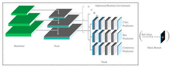
Figure 1.
Overview of Our Architecture Adjustments. Grey convolutions and unsaturated channels are removed to decrease runtime while preserving a good accuracy. The mask branch is improving the detection accuracy during training and can be removed for inference. A centerness prediction branch is applied to delete inaccurate detections which are triggered from a feature map pixel that is far off the detection’s center. Depending on the targeted runtime we use a smaller backbone.
3.1. Base Detection Framework
We adopt RetinaNet as a base detection framework due to its good trade-off between detection accuracy and inference time. As localization and classification is performed in a single stage, the inference time is less compared to two-stage approaches like Faster R-CNN.
RetinaNet is a fully convolutional network that mainly comprises three modules: a backbone network, a feature pyramid network and a classification head. The base network is used as a feature extractor and is generally an off-the-shelf CNN, e.g., ResNet-50. The feature pyramid network, also referred to as neck, is applied on top of the base network to generate semantically rich feature maps. For this purpose, features from deep layers are up-sampled and connected with features from shallow layers via element-wise sum. The classification head is then applied on multiple feature maps in order to account for various object scales. The classification head is composed of two sub-networks: one for classification and one for bounding box regression. Both sub-networks comprise a sequence of 3 × 3 convolutional layers. The classification sub-network outputs at each feature map location the probability of object presence for all classes, while the bounding box regression network predicts class-agnostic bounding box offsets for each feature map location. For this, anchor boxes centered at each feature map location are used as bounding box reference. By default, anchor boxes with three different aspect ratios, i.e., 1:2, 1:1 and 2:1, and three different scales are employed, yielding a total of nine anchor boxes per feature map. Note that differing anchor scales are used for each pyramid level so that the anchor box areas range from pixels on pyramid level P3 to pixels on pyramid level P7. To address the issue of an extreme imbalance between foreground and background classes during training faced by a single-stage detector, RetinaNet applies focal loss as classification loss.
3.2. Adaptations for Improved Detection Accuracy
We perform several modifications of the original RetinaNet to improve the detection accuracy without increasing the inference time.
To account for the small dimensions of occurring objects in aerial imagery, we reduce the anchor box sizes for each pyramid level by setting the anchor base size to 2. Thus, the anchor box size distribution fits better to the GT box size distribution, which generally yields an improved detection accuracy, in particular in case of small objects [35]. Using an auxiliary feature map with higher resolution, i.e., P2, has been rejected because of the significant computational overhead.
We further extend our single-stage detector by adopting the mask branch of Mask R-CNN [15] to exploit more semantic context information and to improve the localization accuracy. The mask branch is applied on top of our single-stage detector similar to the RPN in [11] and outputs a binary segmentation mask for each prediction. For this purpose, a ROI Align layer extracts the corresponding features for each prediction, yielding a small feature map of fixed extent. The small feature map is then passed through a sequence of convolutional layers, and the last layer is used for a pixel-wise classification. By applying an auxiliary loss function termed mask loss , i.e., a binary cross-entropy loss averaged over a prediction’s pixels, the mask branch is trained simultaneously with the classification and bounding box regression. Note that the additional mask branch can be disabled during inference, so that the inference time is not affected.
Due to the imbalanced distribution of occurring classes in aerial imagery datasets, e.g., iSAID [52], we apply the data resampling strategy proposed in [53]. A repeat factor is specified for each training image i:
where are the classes labeled in i and is the fraction of training images that contain at least one instance of class c. The threshold parameter t is a hyper-parameter inserted to control the oversampling.
We further adopt several optimization techniques proposed in [54], i.e., Adaptive Training Sample Selection (ATSS) [54], using the generalized IoU [55] as regression loss, introducing an auxiliary centerness branch [8] and adding a trainable scalar per feature pyramid level [8]. ATSS replaces the traditional IoU-based strategy to define positive and negative samples during training. Instead of using a fixed IoU threshold value to assign positive samples, the IoU threshold is dynamically set based on statistical measures of the IoU thresholds of anchors close to the GT box. While there is no strong correlation between minimizing the commonly used regression losses such as smooth loss and improving the IoU values between GT boxes and predicted boxes, using the metric itself, i.e., IoU, is the optimal objective function [55]. Employing the generalized IoU, which addresses the weakness of the conventional IoU by extending the concept to non-overlapping cases, as regression loss further improves the training and consequently the detection accuracy. The centerness branch is introduced to suppress poorly predicted bounding boxes caused by locations far away from the center of the corresponding object. For this, a centerness score is predicted for each location, which is applied to down-weight the scores of bounding boxes far from the center. For each feature map, the anchor sizes are specified by a fixed scalar termed octave base scale, which is multiplied with the feature map stride. By introducing a trainable scalar per feature map, this value can be automatically adjusted during training, thus allowing for differing anchor sizes. Note that for simplicity we term the optimization techniques proposed in [54] as ATSS. Besides the adopted optimization techniques, group normalization [56] in the classification head has been proposed in [54]. Since the employed TensorRT 6 does not support group normalization, no normalization is performed, which showed superior results compared to applying batch normalization (see Appendix A.1).
3.3. Light-Weight Classification Head
The inference time is mainly affected by the backbone network and the classification head.
While using light-weight network architectures, e.g., PeleeNet or MobileNetV3, as backbone network reduces the inference time, the detection accuracy decreases, in particular for small object instances. Thus, we employ ResNet-50 as backbone network, which showed, among various network architectures, the best trade-off between detection accuracy and inference time.
The large computational costs of the classification head is caused by the sequences of four convolutional layers in the sub-networks. The number of multiply-add computations (MACs) of a convolutional layer depends on the kernel size , the number of kernels C, the number of input channels D and the output width W and height H:
We lower the number of input channels and the number of kernels from 256 to 170, respectively, which reduces the number of MAC operations by roughly 56%. For this, we set the depth of each feature map to 170 as well. Furthermore, we discard the last convolutional layer, which reduces the computational costs by additional 25%. Preliminary experiments showed that our light-weight classification head yields the best trade-off between inference time and detection accuracy.
3.4. Adapted Runtime Environment
As runtime environment, we make use of NVIDIA’s TensorRT library instead of the original deep learning framework MMDetection based on PyTorch, which notably reduces the inference time. For this, we convert our PyTorch model to ONNX format, which is then parsed to TensorRT. To further speed-up the inference, we use TensorRT’s FP16 arithmetic instead of the usual FP32.
Besides ONNX, torch2trt (https://github.com/NVIDIA-AI-IOT/torch2trt, accessed at 3 April 2021) and TRTorch (https://github.com/NVIDIA/TRTorch, accessed at 3 April 2021) exist as paths to convert models from PyTorch to TensorRT. Torch2trt implements its own tracing mechanism to directly build the TensorRT network based of PyTorch operations. TRTorch is a converter from TorchScript to TensorRT and thus relies on PyTorch’s tracing and scripting mechanisms to convert PyTorch operations to TorchScript. However, ONNX is still the most established conversion path. While the conversion process might not seem to need a lot of effort, in practice, some functionality is lacking and manual optimization is required for good performance as described below. Thus, a lot of manual effort is still required as can also be seen from other projects porting MMDetection to TensorRT (https://github.com/grimoire/mmdetection-to-tensorrt, accessed at 3 April 2021).
Since the non-maximum suppression (NMS) of ONNX has a dynamically sized tensor as output, TensorRT does not provide an implementation of the ONNX NMS. Thus, we define a custom ONNX node that uses two fixed size outputs so that it is compatible with the output format of TensorRT’s NMS. The first output is a tensor, which has space for 1000 detections and the second tensor describes the number of valid detections in the first tensor. Additionally, we add a parser for the new node type to the ONNX-to-TensorRT converter.
MMDetection’s ATSS implementation filters the detections based on their classification score and multiplies the centerness score with the classification score prior to the NMS. In case of TensorRT, the filtering based on the classification score and the NMS are by default done in a single step. As TensorRT’s NMS does not handle different score types, we multiply the centerness score before the NMS and halve the score threshold for the filtering to cope with the reduced absolute score values. Ignoring the centerness score would be a clearly inferior solution.
To reduce the inference time, we use the TensorRT profiler to find opportunities for optimization. One step which takes exceptionally long is the extraction of the bounding boxes from the feature maps. When all convolutions have been executed, five tensors exist from the different octaves. In MMDetection and therefore also in the converted model, even for batch size 1 these tensors contain a dimension for the batch size. However, for the output a single tensor containing all detections for a single image has to be created. Thus, for each image of the batch, the feature map has to be extracted, flattened, and afterwards concatenated with the detections from the other octaves. The code in Listing 1 is used for the extraction in MMDetection.
However, when exporting this code to ONNX, a Gather node is created which has a relatively high inference time with TensorRT. Thus, we replace the code with the code from Listing 2 which generates a Squeeze node in the exported ONNX file. Running RetinaNet with the older version result in 13.9 FPS while the new version is running at 14.6 FPS. While the shown code only handles the feature maps for class prediction, the same principle applies to the feature maps for regression and centerness prediction.

Listing 1: Original MMDetection Code for Extracting Feature Maps.
Listing 1: Original MMDetection Code for Extracting Feature Maps.
| [ cls_scores [ i ][img_id].detach() for i in range(num_levels) ] |
Listing 2: Adjusted Code for Extracting Feature Maps.
Listing 2: Adjusted Code for Extracting Feature Maps.
| [ torch.squeeze(cls_scores[i ]) .detach() for i in range(num_levels) ] |
4. Experimental Results
In this section, we first provide the experimental settings and introduce the applied evaluation metrics. Then, we compare different configurations of our proposed object detector to work published on iSAID and to state-of-the-art object detectors fine-tuned on iSAID. Next, we provide an ablation study to highlight the impact of the proposed techniques to optimize the detection accuracy without affecting the inference time followed by an analysis of the proposed light-weight classification head. Finally, the main settings of our final configurations are given and qualitative examples are shown.
4.1. Experimental Setup
For our experiments, we use the iSAID dataset [52] that comprises 2806 aerial images with more than 650k annotated object instances for 15 classes. While most classes are very different and are thus a challenge for the detection of objects, small vehicles and large vehicles are very close in its appearances and are highly difficult to distinguish. Another major difficulty for detecting objects in the images are the large range of GSDs (1.0 m to 4.5 m) of the images included in the iSAID. A subset of the classes in iSAID and the different ground sampling distances are shown exemplary in Figure 2. Moreover, the many small objects in the iSAID are a challenge for embedded real-time detectors since large input images and large feature maps lead to an increased runtime. As can be seen in Figure 3, this is different to datasets like MS-COCO [57] which are mainly used in object detection research and are lacking this difficulty. As annotations are not publicly available for the test set, we only use the official training and validation set for our experiments. The training and validation set comprise 1411 and 458 images, respectively. For each set, the histogram of the number of instances per class is given in Figure 4.
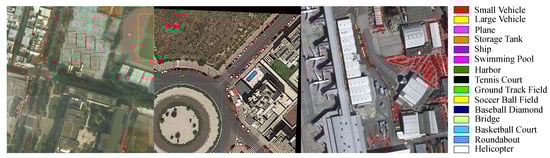
Figure 2.
Three images from iSAID. The first image shows the high variety in appearance and size of the classes in iSAID. The second and third images show the high difference in terms of GSD. The color coding for the classes is applied in all figures.
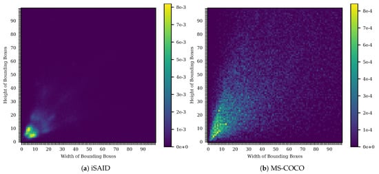
Figure 3.
Distribution of object sizes in iSAID [52] (a) and MS-COCO [57] (b). The distribution of iSAID is heavily skewed towards small objects. Thus a focus on the small objects is needed. However, even though large objects are rare, each of them is more important for the average precision since they are typically in rare classes. This discrepancy combined with the many small and thus hard to detect objects poses a major challenge for the detector.
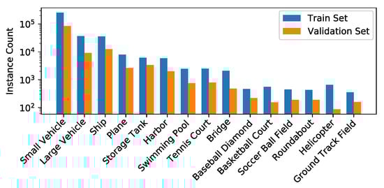
Figure 4.
Histogram of the number of instances per class.
We train all models on cropped images with a size of pixels that are extracted from the original training set with a sliding window approach. Note that the baseline detectors are trained on a set of cropped images that have an overlap of 200 pixels as provided by [52], while our ablation studies are based on models trained on a set that uses an overlap of 400 pixels and cropped ground truth objects with an IoU less than 50% to the original GT bounding box are discarded. During training multi-scale augmentation ranging from 50% to 150% and horizontal flip augmentation are used.
The baseline detectors shown in Table 1 and the ablation studies are trained with a batch size of 4 and stochastic gradient descent as optimizer using an initial learning rate of 1 × 10. Note that we restart the training with a lower learning rate, i.e., 5 × 10, if the training diverges. We use the NMS settings recommended by [52]. The training settings for our final models are described in Section 4.5.
Table 1.
Comparison of our proposed object detector to different state-of-the-art detectors. Even though the compared detectors are close in terms of accuracy, our detectors have a significantly higher frame rate. The increased accuracy compared to the baseline RetinaNet are due to the multiple improvements mentioned in Section 3.2. The main reasons for the increased performance of the 15 FPS model are the application of TensorRT and half-precision floating-point. The faster models benefit from carefully scaling the backbone, the head and the resolution.
Following [52], we use the standard MS COCO metrics to evaluate the detection accuracy: AP (averaged over IoU thresholds in the range between 0.5 and 0.95), , , , and , with the area ranges for S, M and L being adjusted according to [52]. The inference time is reported in frames per second (FPS). Faster R-CNN, RetinaNet and Mask R-CNN are evaluated with MMDetection [58], EfficientDet is evaluated with AutoML and YOLOv4 is evaluated with DarkNet. All ablation studies and our final models are evaluated with TensorRT 6 and 16-bit floating point. Because of the high effort needed to port models to TensorRT and since the porting process typically involves modifications to the model not part of the original model, we refrain from using TensorRT and FP16 for the baseline models. However, at least the models implemented in MMDetection would likely profit. We use MMDetection 1.0, PyTorch 1.3 [59], ONNX opset 10 and TensorRT 6 [60]. The experiments are run on a Nvidia Jetson AGX Xavier using JetPack 4.3 and the 30 W power mode with two CPU cores enabled and the clock frequencies fixed to the power mode’s maximum values.
4.2. Baseline Experiments
The results of our proposed models compared to baseline detectors on the iSAID validation set are shown in Table 1. The best result for each column is marked bold. The first part of the table shows results of baseline detectors and the second part provides results of our optimized models.
The evaluated baseline detectors are Faster R-CNN, RetinaNet, Mask R-CNN, EfficientDet D2 and YOLOv4 with the first three being widely adopted object detectors and the latter two being state-of-the-art models for mobile object detection. Faster R-CNN is a two-stage model that predicts region proposal and afterwards classifies them in a second stage. RetinaNet is a modern one-stage detector that applies a focal loss to handle the high class-imbalance between foreground and background. Mask R-CNN extends Faster R-CNN by a mask branch to predict instance segmentation. EfficientDet is a one-stage detector that employs a modern EfficientNet [48] backbone and a BiFPN neck with multiple consecutive top-down and bottom-up paths. YOLOv4 is a one-stage detector which uses a cross stage partial network [62], spatial attention and heavy data augmentation.
Amongst the baseline detectors, Mask R-CNN achieves the best AP. Using the PA-FPN as neck similar to PANet shows no improvement. The best inference time (evaluated without TensorRT) is achieved for EfficientDet followed by YOLOv4 and RetinaNet. However, EfficientDet exhibits a poor AP and one reason for the superior inference time is the TensorFlow environment. Thus, we decided to use RetinaNet as base detector since the two-stage models are more complex to deploy and YOLOv4 is not available in MMDetection, which limits the possibility to evaluate different configurations. Overall, we propose four models optimized for different frame rates, i.e., 15 FPS, 30 FPS, 60 FPS and 90 FPS. Our model that runs at 15 FPS achieves the best AP and clearly outperforms the baseline detectors in AP and FPS.
The results of our proposed models compared to published results on the iSAID test set are shown in Table 2. Though the proposed model comprises a smaller backbone and neck to ensure a fast inference time, the AP is close to the AP achieved for PANet. Since the evaluation server for the test set only supports a limited amount of detections, we can not apply our optimization of a reduced score threshold as mentioned in Section 4.3. Thus, our results on the test set as presented are lower compared to a normal evaluation.
Table 2.
Comparison of our proposed object detector to different results published for the iSAID. All evaluations are executed on the test set.
4.3. Adjustments Not Impacting the Runtime
In the following, TensorRT and FP16 are used for all experiments. The advantage of using TensorRT over MMDetection and reducing the data precision is shown for RetinaNet in Table 3. Using TensorRT and FP16 speeds up the inference time by a factor of about 5, while the detection accuracy is almost unchanged. The AP values differing from the AP value reported in Table 1 are due to more training data used for the ablation study as described above.
Table 3.
Comparing RetinaNet evaluated with MMDetection and TensorRT and different floating point precisions. Both applying TensorRT and reducing the precision to 16 bit is slightly increasing the runtime. However, applying both optimizations increases the runtime by a multiple while not impacting the accuracy.
In the following subesction, we evaluate multiple optimizations that improve the accuracy while not impacting the runtime or only impacting it slightly. These optimizations are
- Adjusting the Anchor Box Size
- Adopting ATSS
- Class-Balanced Training
- Denser Cropping Strategy
- Auxiliary Mask Branch
- Adopting AdamW Optimizer
Adjusting the Anchor Box Sizes: Reasons for the higher AP values of Faster R-CNN and Mask R-CNN compared to RetinaNet, in particular for small object instances (see Table 1), are the employed feature maps and the size of the corresponding anchor boxes. By default, RetinaNet uses the outputs from the feature pyramid levels P3 to P7 as feature maps for prediction. Faster R-CNN and Mask R-CNN take the output from feature pyramid level P2 as auxiliary feature map. The corresponding anchor boxes are in the range of pixels and thus, smaller compared to the anchor boxes employed for RetinaNet. In the following, we evaluate the impact of using an auxiliary feature map with higher resolution, i.e., P2, and of reducing the anchor box sizes by varying the octave base scale (see Table 4). While using P2 provides the best accuracy, it more than halves the FPS due to the computational overhead. Setting the octave base scale to 2, which yields anchor boxes in the range of pixels, exhibits an almost similar improvement without impacting the runtime. Thus, we reduce the octave base scale from 4 to 2 (8 to 4 for experiments with ATSS) for our experiments and the final models.
Table 4.
Comparison of RetinaNet with varying octave base scales and different feature maps. Note that start and end indicate the first and last pyramid level used as feature map. Reducing the smallest anchor by either reducing the anchors’ base size or incorporating an earlier feature map in the detection head to accommodate the many small objects increases the AP. While incorporating an earlier feature map leads to the best average precision, it heavily impairs the FPS because of the processing of the high resolution feature map.
Adopting ATSS: As can be seen in Table 5, adopting ATSS (Section 3.2) provides a great advantage in terms of accuracy over the original RetinaNet. The AP increases by 2.5 points and another 0.1 points can be gained by lowering the score threshold to compensate the centerness score. ATSS also increases the FPS from 14.8 to 15.7 since it typically uses only one anchor while RetinaNet uses nine anchors with three different aspect ratios and three different scales.
Table 5.
Comparison of RetinaNet with and without ATSS. The centerness score prediction is typically applied after filtering low confidence detections. However, the TensorRT NMS has not support for such an operation. Thus, we evaluate both multiplying the centerness score before filtering detections and ignoring the centerness score. Both variants significantly increase the precision compared to not applying ATSS while multiplying the centerness score with the class score prediction before the filtering procedure shows a higher precision. To accommodate the lower scores, we reduce the score threshold which slightly increases the precision. All variants with ATSS significantly increase the FPS since ATSS uses only 1 anchor instead of 9.
Class-Balanced Training: The classes in iSAID are highly unbalanced, e.g., the number of small vehicles is about 1500 times the number of ground track fields. This leads to frequent classes generating a large part of loss, while less frequent classes have a smaller contribution to the weight adjustments. However, the AP is weighting less frequent classes equally to frequent classes. By applying the data resampling strategy described in Section 3.2 to increase the contribution of less frequent classes to the loss, we increase the AP by 2.6 points (see Table 6). For this, the oversampling threshold is set to 0.1. The impact on the class-wise detection results is shown in Table 7. As expected, the rare classes are having the greatest improvement with helicopter being detected twice as good. However, even highly frequent classes like small vehicle show a slight improvement. We assume that this is due to rare classes producing a smaller loss per annotation with class-balanced training since the prediction is more accurate and thus causing less adjustments negatively impacting the accuracy of frequent classes. Ship is the only class which has a slightly lower AP when using class-balanced training.
Table 6.
Comparison of dataset preparation settings, i.e., w/ and w/o discarding of boxes with low IoU to the original box in the uncropped image and class-balanced resampling. The third line is the default data preparation strategy proposed by [52]. To prevent confusing the detector by unidentifiable objects during training, we discard objects which have a visibility of less than 50% in the experiments for the ablation studies. However, since the validation set includes such objects, discarding impairs the performance. The denser cropping strategy with only 200 pixel overlap in the application of the sliding window significantly increases the precision.
Table 7.
Class-wise results comparing RetinaNet with and without class-balanced sampling. Even though the rare classes like Helicopter are obviously benefiting most from the oversampling of the images including them, frequent classes like small vehicles also show a better precision. Ship is the only class that is slightly impaired by the class-balancing. Abbreviations: BD—Baseball Diamond, GTF—Ground Track Field, SV—Small Vehicle, LV—Large Vehicle, TC—Tennis Court, BC—Basketball Court, ST—Storage Tank, SBF—Soccer Ball Field, RA—Roundabout, SP—Swimming Pool, HC—Helicopter.
Denser Cropping Strategy: Furthermore, we examine the impact of different settings to crop the original images during training. Using an overlap of 400 pixels instead of the initially applied 200 pixels results in an improved detection accuracy, as clearly more training samples are considered. However, discarding bounding boxes whose overlap to its original bounding box is below 50% shows no gain in AP and thus, is not applied for further experiments.
Auxiliary Mask Branch: Additionally, we evaluate the impact of an auxiliary mask branch. For this, the same number of convolutions and channels are used as for the classification head. The results of applying the mask branch for different input image resolutions are shown in Table 8. It can be seen that the auxiliary mask branch increases the AP over all tested resolutions by 1.2 to 1.6 points.
Table 8.
Comparing RetinaNet with auxiliary mask branch and without mask branch for different input resolutions. Across all resolutions the auxiliary mask branch is showing a significant increase in precision while not impairing the FPS since it is not executed during inference.
Adopting AdamW Optimizer: Finally, we evaluate different optimizers in Table 9. Since Adam-based optimizers usually work best with lower learning rates, we reduce the learning rate for these. The tests are conducted using RetinaNet with Mask Branch. Adam results in an increase of 1.5 points average precision over SGD and AdamW leads to another 0.7 point increase.
Table 9.
Comparing different optimization algorithms on RetinaNet. Since Adam-based optimizers typically require a lower learning rate, we execute Adam and AdamW with a learning rate of 1 × 10 instead of 1 × 10. Adam shows a significant increase in terms of precision compared to SGD and AdamW further increases the precision slightly.
4.4. Optimizing the Accuracy-Runtime Trade-Off
To optimize the trade-off between detection accuracy and inference time, we initially analyze the impact of each detector component on the overall inference time (see Table 10). For this, the runtime of each component is separately measured using the TensorRT profiler. The largest portion of the runtime are spent on the backbone and the classification head with 43% and 45%, respectively, while the neck only requires 9% of the total time. The time spent for the NMS is almost negligible with only 1%. Note that some layers like copy operations that are added by TensorRT can not be traced back to the original components and thus, these layers are termed unassigned.
Table 10.
Runtimes of RetinaNet’s components. Due to technical reasons some operations could not be assigned to a certain component. The backbone and the head are the two significant parts sharing almost 90% of the runtime equally. The remaining share is mainly consumed by the neck.
At first, we examine the usage of different backbone networks in Figure 5. Even though multiple modern architectures are used to replace ResNet [65] as backbone, ResNet still offers the best trade-off between detection accuracy and runtime. While certain configurations of RegNetX [66] are a suitable alternative to ResNet, using light-weight networks, e.g., PeleeNet [49], MobileNetV3-Large [45] and EfficientNet [48] results in clearly worse AP. Backbones targeted towards a high accuracy like ResNeXt [67] or HRNetV2 [68] also provide an inferior trade-off between detection accuracy and runtime compared to ResNet.
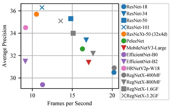
Figure 5.
Comparing RetinaNet with different backbones. The ResNet family shows a good accuracy-runtime-trade-off in almost all circumstances. Only in the high FPS regime RegNetX achieves a higher precision with the same runtime comaped to ResNet-18. However, further experiments have shown that ResNet-18 is better when other improvements are also applied.
Thus, our focus lies on optimizing the inference time spent for the classification head by reducing the number of stacked convolutions and the number of channels as described in Section 3.4. Results for different configurations of number of stacked convolutions and number of channels are shown in Table 11. The best trade-offs between inference time and detection accuracy are achieved for 3 stacked convolutions and 170 channels and 2 stacked convolutions and 128 channels, respectively. Removing more convolutions or channels results in worse AP. Note that a balanced adaption of these parameters is appropriate to avoid a large drop in AP. The impact of reducing the resolution as a further scaling factor is shown in Figure 6. For each configuration, the input image resolution is varied between and pixels. Decreasing the input image resolution to pixels shows a large speed up with only a small drop in AP for all configurations, while for an input image resolution of pixels the AP becomes considerably worse.
Table 11.
Comparing RetinaNet (ResNet-50 and ResNet-18) with different head and neck configurations. The first two steps of downscaling the head and the neck lead to a significant speed-up with both backbones while only slightly impairing the precision. Further reducing the number of channels to 64 and removing all stacked convolutions in the head leads to a significant drop in accuracy. Thus we do not consider this setting for further experiments.
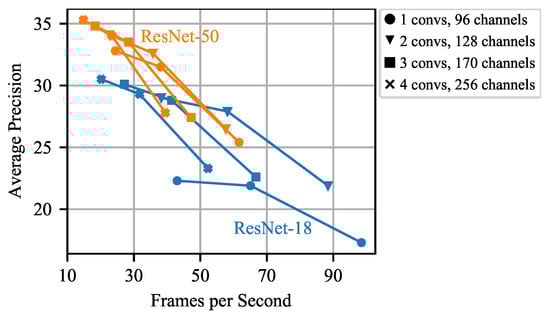
Figure 6.
Comparison of different classification head settings, i.e., number of stacked convolutions and number of channels, for input images of size (left), (middle) and (right). Reducing the resolution to impairs the precision only slightly while the accuracy is significantly increased. Further reducing it to decreases the precision heavily for large model configurations. However, for small model configurations the relative impairment is lower while still significantly increasing the frame rate. Thus, both steps are considered for selecting the final models.
4.5. Selecting Final Models
For the final models, we adopt an octave base scale of 2 to account for small object instances and apply ATSS, an auxiliary mask branch during training and class-balanced dataset augmentation. Based on the results from Figure 6, we choose the configurations for the final models as shown in Table 12. The four models differ in the size of the backbone (ResNet-50 or ResNet-18), the number of channels in the neck and the head (256, 170 or 128), the number of stacked convolutions before the final prediction in the head (4, 3 or 2) and the resolution of the input image (800 × 800, 600 × 600, 400 × 400). Note that AdamW is used as optimizer with a learning rate of 1 × 10, which slightly improves the detection accuracy as shown in further experiments with the final configurations. Qualitative results of our proposed models compared to the GT indicate the good localization and classification accuracy even at high frame rates (see Figure 7).
Table 12.
Selected model configuration for each of the four targeted frame rates. Channels are the number of channels in the neck and in the head. Convolutions are the number of stacked convolutions in the head. For each targeted frame rate the most precise configuration is selected from Figure 6.
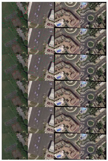
Figure 7.
Qualitative results of our 15 FPS model (second row), 30 FPS model (third row), 60 FPS model (fourth row) and 90 FPS model (fifth row) compared to RetinaNet (bottom row) and ground truth annotations (top row). These results approve the quantitative results with the faster models dropping in accuracy because of more missed objects. While RetinaNet does not miss many objects, it outputs many false positive predictions which leads to its poor quantitative results.
4.6. Power and Memory Measurement
The power consumption and the required VRAM of each model is shown in Table 13. Note that the average power is an average over the complete inference including loading the images, while the model power is the average drawn power without loading the images. All power consumption results are averaged over three runs. All models consume significantly less power than specified by the power mode since not all processing units are fully utilized. As a result, the clock frequencies and thus, the FPS could be increased without exceeding the power limit.
Table 13.
Power consumption and required VRAM of the four models in 30 W power mode. Average power is the total power measured during inference including loading images. Model power is the power averaged over the raw model execution, i.e., the power needed for loading images is subtracted. The required power is significantly below the configured 30 W limit since not all of Jetson’s processing units are utilized. Moreover, the power draw decreases with a higher frame rate since the utilization of the high-power GPU decreases. The required VRAM decreases for the faster models since the smaller number of feature maps have a lower resolution and the smaller models have less parameters.
The VRAM required for executing the models is decreasing for the faster and smaller models since they use less feature maps. Moreover, due to the smaller input resolution, the input image has a smaller memory footprints and all feature maps also have a lower resolution. Additionally, the smaller models have a lower number of parameters which need to be kept in memory. However, even the 15 FPS model only requires about 1.7 GiB of VRAM and can thus be also executed on devices offering drastically lower capabilities than the tested Jetson AGX Xavier.
5. Oriented Bounding Boxes
Oriented object detection in aerial imagery is of rising interest, since horizontal bounding boxes (HBBs) might not fit the requirements of certain applications. However, works on oriented object detection in aerial imagery only focus on improving the detection accuracy, while the impact of the applied modifications on the inference time are not considered. In the context of this work, we examine the inference time of oriented object detection on a Nvidia Jetson AGX Xavier as example for a mobile device. For this purpose, we evaluate two different schemes to predict OBBs, i.e., adding a fifth parameter in the regression representing the bounding box’ angle and a regression type based on eight parameters representing the coordinates of the corners. For the first scheme, we further apply modulated loss [69], which prevents the loss from punishing the network for predicting almost correct bounding boxes in terms of IoU but with a different representation than the GT box. Note that iSAID contains no annotations for OBBs. Thus, we create the oriented annotations by calculating the minimal surrounding bounding box based on the segmentation mask of each object.
Our implementation is based on Aerial Detection (https://github.com/dingjiansw101/AerialDetection/, accessed at 3 April 2021) which extends MMDetection with detection heads for oriented bounding boxes. Table 14 shows the detection results for oriented object detection. Compared to the results for the horizontal counterpart, the AP drops from 38.3 to 27.6 in the best case, which indicates that oriented object detection is a significantly more difficult task than predicting HBBs. Among the evaluated OBB detectors, the five-parameter configuration including modulated loss has the highest accuracy and thus, is used for further experiments.
Table 14.
Comparing RetinaNet predicting horizontal bounding boxes (HBBs) and oriented bounding boxes (OBBs) in different configurations. Both bounding box types are trained and evaluated on their respective dataset type. While the AP is heavily impaired, the AP50 is only slightly reduced when predicting OBBs since the precise estimation of the angle is not important for objects with a ratio close to 1 to achieve an IoU above 50%. Among the tested configurations, predicting the usual bounding box parameter and an angle while using modulated loss to handle angle periodicity achieves the best results.
Bottleneck of the deployment of oriented object detection on embedded devices is the NMS, since the skew IoU computation [70] between two OBBs is much more complicated than the regular IoU computation for HBBs. As TensorRT provides no NMS for OBBs, we implement it by ourselves. Generally, surrounding HBBs are generated for a pair of OBBs and their IoU is computed. If no IoU exists, the skew IoU does not need to be computed. However, since only some boxes need the skew IoU computation while others does not, this leads to a high branch divergence when parallelizing the NMS which is unfavorable for GPUs. Thus, we propose to not only parallelize the NMS on bounding box level but also parallelize each skewed IoU computation by making use of the pairwise intersection calculation of both bounding boxes’ lines which are 16 independent computations. This leads to a higher warp utilization since at least 16 of the 32 threads of a warp are used. Without this extended parallelization, it can happen that only a single thread out of 32 is used. Since the assignment of warps is fixed, the unused shader cores cannot be used by other threads. The impact of this optimization is shown in Table 15. Increasing the IoU threshold applied for the check of the surrounding HBBs boosts the inference time. While this is not an optimal solution in terms of correctness, it reduces the number of boxes that require a skew IoU computation. With the parallelized skew IoU computation and increasing the horizontal IoU threshold to 60 %, RetinaNet predicting OBBs is only 4.4 ms slower per image than a default RetinaNet.
Table 15.
Evaluating the impact of parallelizing the skew IoU computation and increasing the IoU threshold used for checking for a horizontal overlap. Without further optimizations, the NMS becomes a bottleneck when predicting OBBs and reduces the advantage of TensorRT and half-precision floating-point arithmetics. Parallelizing the skew IoU to increase the GPU utilization and only calculating the skew IoU if a significant horizontal IoU is given, increases the performance to a level close to HBB prediction.
Figure 8 shows that the oriented bounding boxes are correctly predicted for both small objects like cars and large objects such as tennis courts.
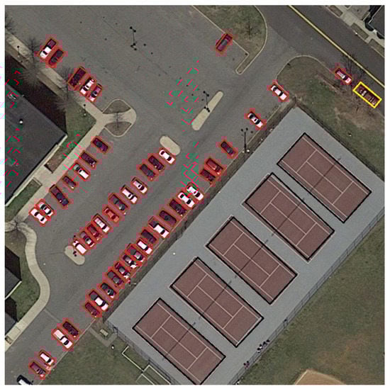
Figure 8.
Qualitative result of RetinaNet predicting oriented bounding boxes. The resulting predictions are almost perfect. Longish objects which are not axis-aligned have a much tighter bounding box when predicting OBBs compared to HBBs. This also reduces the risk of the NMS dropping correct bounding boxes because of a high overlap.
6. Conclusions
In this work, we present a workflow for optimizing object detection models to enable real-time processing with low power consumption. The four steps of this workflow are: initial model selection, accuracy optimization, runtime optimization and deployment optimization. We executed this workflow exemplary for object detection in aerial imagery and thereby proved the effectiveness of this workflow. Our final models provide a good trade-off between accuracy and runtime with the 30 FPS model operating at real-time on an embedded device. State-of-the-art models are outperformed in terms of inference time, while still achieving a similar accuracy.
A denser cropping policy for creating the training images proved to be the single most important aspect for improving the accuracy. Sampling the images in a class-balanced manner, adapting the ATSS including a centerness prediction branch and the generalized IoU loss and adjusting the anchor sizes to the small objects in the iSAID also proved to have a highly positive impact on the accuracy. However, replacing the default SGD optimizer with AdamW and applying a mask branch during training also show a significant improvement in terms of accuracy.
To optimize the detection architecture for runtime the head is the most import component which can be shrunken with a small reduction of the accuracy with a comparative high reduction in terms of runtime. Another important aspect for a better accuracy-runtime-trade-off is the resolution of the input images which should be reduced. Besides the head, the backbone also demands a large share of the runtime. However, more modern backbones do not prove advantageous over the ResNet family and choosing smaller backbones cause a significant drop in accuracy. Thus, we choose them only for the models with 60 FPS or more.
To enable real-time object detection with oriented bounding boxes, we identify the NMS as the main drawback and apply two optimizations to it. First, we parallelize the IoU calculation to increase the GPU utilization. Second, we apply a higher horizontal IoU threshold that must be exceed before the oriented IoU is considered. This optimization significantly reduces the required workload.
Still to be investigated is the performance on different hardware and the potential of integer quantization with 8 bits and below. To increase the accuracy without loosing performance more data augmentation could be considered, e.g., copy-and-paste [71]. To improve the detection with oriented bounding boxes, the optimizations applied for horizontal detections like ATSS and mask branch should be adopted. Furthermore, oriented object detection is typically approached by two-stage pipelines. Thus, the deployment of such two-stage pipelines with TensorRT should be considered.
Author Contributions
Conceptualization, L.S. and A.S.; methodology S.W.; software S.W.; investigation S.W.; resources L.S. and A.S.; writing—original draft preparation, S.W., L.S. and A.S.; writing—review and editing, S.W., L.S. and A.S.; visualization, S.W.; supervision, L.S. and A.S.; project administration, L.S. and A.S.; funding acquisition, A.S. All authors have read and agreed to the published version of the manuscript.
Funding
The APC was funded by Fraunhofer-Gesellschaft and Fraunhofer Institute of Optronics, System Technologies and Image Exploitation IOSB.
Institutional Review Board Statement
Not applicable.
Informed Consent Statement
Not applicable.
Data Availability Statement
Publicly available datasets were analyzed in this study. This data can be found here: https://captain-whu.github.io/iSAID/, accessed at 3 April 2021.
Conflicts of Interest
The authors declare no conflict of interest.
Abbreviations
The following abbreviations are used in this manuscript:
| AP | Average Precision |
| ATSS | Adaptive Training Sample Selection |
| CNN | Convolutional Neural Network |
| CPU | Central Processing Unit |
| DSSD | Deconvolutional SSD |
| FastAER Det | Fast Aerial Embedded Real-Time Detector |
| FCOS | Fully Convolutional One-Stage Object Detector |
| FP16 | Floating Point 16 |
| FP32 | Floating Point 32 |
| FPN | Feature Pyramid Network |
| FPS | Frames Per Second |
| GPU | Graphics Processing Unit |
| GSD | Ground Sampling Distance |
| GT | Ground Truth |
| HBB | Horizontal Bounding Box |
| IoU | Intersection over Union |
| iSAID | Instance Segmentation in Aerial Images Dataset |
| MAC | Multiply-Add Computation |
| MDPI | Multidisciplinary Digital Publishing Institute |
| MS-COCO | Microsoft Common Objects in Context |
| NMS | Non-Maximum Suppression |
| OBB | Oriented Bounding Box |
| ONNX | Open Neural Network eXchange |
| PA-FPN | Path Aggregation Feature Pyramid Network |
| PANet | Path Aggregation Network |
| R-CNN | Region Based Convolutional Neural Network |
| ROI | Region of Interest |
| RPN | Region Proposal Network |
| SGD | Stochastic Gradient Descent |
| SSD | Single Shot MultiBox Detector |
| SSSD | Simple Short and Shallow Network |
| UAV | Unmanned Aerial Vehicle |
| YOLO | You Only Look Once |
Appendix A
Appendix A.1. ATSS Experiments
Zhang et al. [54] propose to use ATSS with group normalization in the head. However, because of the lack of group normalization support in TensorRT 6, we need to either use batch normalization or no normalization in the head. Thus, we evaluate all three normalization types in Table A1. Using batch normalization results in an average precision of 1. Thus, we decide to use no normalization which results in 38 points. This result is even 0.3 points better than group normalization.
Table A1.
Comparing ATSS with different normalization types in the head. Evaluation done with MMDetection. ATSS typically applies group normalization. However, group normalization is not supported by TensorRT 6. Thus, we evaluate batch normalization and applying no normalization as alternatives. However, batch normalization is not working at all even if the batch size is increased.
| Normalization | AP | AP50 | AP75 | APs | APm | APl |
|---|---|---|---|---|---|---|
| Group Normalization | 37.7 | 59.7 | 40.5 | 40.3 | 43.7 | 48.6 |
| Batch Normalization | 1.0 | 1.9 | 1.0 | 1.1 | 0.4 | 0.0 |
| Batch Normalization (Batch Size 8) | 1.6 | 2.9 | 1.6 | 1.8 | 0.0 | 0.0 |
| No Normalization | 38.0 | 58.9 | 41.2 | 40.4 | 45.2 | 55.4 |
Appendix A.2. Head Experiments
In Figure A1, a comparison of different resolutions, backbones and head configurations is shown. In contrast to the comparison in Figure 6, this also includes ResNet-34 and a smaller head configuration.
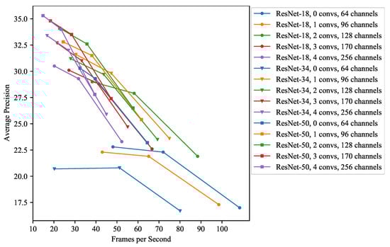
Figure A1.
Comparing RetinaNet in different configurations with different input resolutions. Convs are the number of stacked convolutions in the head. Channels are the number of channels in the head and in the neck. The left point of each series is , the middle point is and the right point is .
Figure A1.
Comparing RetinaNet in different configurations with different input resolutions. Convs are the number of stacked convolutions in the head. Channels are the number of channels in the head and in the neck. The left point of each series is , the middle point is and the right point is .
Appendix A.3. Non-Maximum Suppression Hyper Parameters
In this section, we evaluate the selection of hyper parameters for the NMS. Three parameters control the maximum number of detections during the NMS processing. The first parameter is the layer-wise pre-NMS maximum which is applied per octave layer before the NMS. Thereafter, the global pre-NMS maximum limits the total number of detections that are used as input for the NMS. After the NMS, the post-NMS maximum is applied. We first evaluate reducing the post-NMS maximum below 1000 and show the results in Figure A2a. While the number of objects have a large impact on the accuracy, the impact on the FPS is negligible. Thus, a reduction of post-NMS maximum is not sensible. Increasing the post-NMS maximum above 1000 is only sensible when we also increase the pre-NMS maximums. In Table A2, we show the result of different configurations of all three parameters. The results indicate that the model is rather insensitive to changes in the range of values larger than 1000. Even tough small increases in the average precision can be gained, this also increases the inference time and makes the trade-off questionable. Thus, we decided to use 1000 for all three parameters.
Table A2.
Comparing impact of maximum number of detections before and after NMS processing on accuracy and inference time. The number of detections is limited per neck layer before the NMS, after concatenating detections from all neck layers but before applying NMS and after applying NMS. While increasing the maximum number of detections increases the precision, it impairs the performance in similar ratio and does not provide a benefit in terms of accuracy-runtime-trade-off.
| Maximum | AP | AP50 | AP75 | APs | APm | APl | FPS | ||
|---|---|---|---|---|---|---|---|---|---|
| Layer-Wise Pre-NMS | Global Pre-NMS | Post-NMS | |||||||
| 1000 | 1000 | 1000 | 35.3 | 58.4 | 37.2 | 37.9 | 38.8 | 21.9 | 14.8 |
| 1000 | 2000 | 1000 | 35.4 | 58.6 | 37.3 | 38.1 | 38.9 | 21.9 | 14.7 |
| 1000 | 2000 | 2000 | 35.4 | 58.7 | 37.3 | 38.1 | 38.8 | 21.9 | 14.7 |
| 2000 | 2000 | 2000 | 35.5 | 58.9 | 37.4 | 38.2 | 38.8 | 21.9 | 14.6 |
Another hyper parameter of the NMS is the IoU threshold that two boxes of the same class need to exceed to discard one of them. We evaluate this parameter in the range of 0.4 to 0.7. The results for HBBs are shown in Figure A2b and the results for OBBs are shown in Figure A2c. For both bounding box types, the values 0.5 and 0.6 are optimal. However, the average precision is overall rather insensitive to the changes in the IoU threshold in the range of the tested values. While the impact on the FPS is negligible for the HBBs, it has a small impact on the FPS for the HBBs with a lower IoU threshold being faster since more boxes are discarded early.
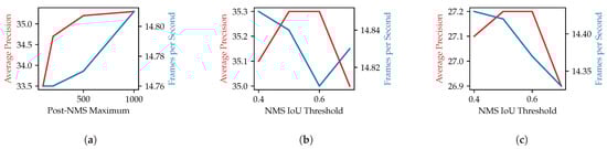
Figure A2.
Results for adjusting NMS hyper parameters. (a) Comparing impact of maximum number of detections after NMS processing on accuracy and inference time. Reducing the number of detections to 500 is a good trade-off if the maximum performance of a model is needed. However, further reduction significantly impairs the precision with a small benefit in terms of performance. (b) Comparing impact of the IoU threshold of the NMS on accuracy and inference time. The impact of the IoU threshold is rather small both in terms of precision and performance if it is in a reasonable range between 0.4 and 0.7. (c) Comparing impact of the IoU threshold of the NMS in terms of accuracy and inference time for detecting oriented bounding boxes. Similar to the prediction of HBBs is the impact only marginal.
References
- Liu, W.; Anguelov, D.; Erhan, D.; Szegedy, C.; Reed, S.; Fu, C.Y.; Berg, A.C. Ssd: Single shot multibox detector. In Proceedings of the European Conference On Computer Vision, Amsterdam, The Netherlands, 8–16 October 2016; pp. 21–37. [Google Scholar]
- Redmon, J.; Divvala, S.; Girshick, R.; Farhadi, A. You only look once: Unified, real-time object detection. In Proceedings of the IEEE Conference on Computer Vision and Pattern Recognition, Las Vegas, NV, USA, 27–30 June 2016; pp. 779–788. [Google Scholar]
- Fu, C.Y.; Liu, W.; Ranga, A.; Tyagi, A.; Berg, A.C. Dssd: Deconvolutional single shot detector. arXiv 2017, arXiv:1701.06659. [Google Scholar]
- Lin, T.Y.; Goyal, P.; Girshick, R.; He, K.; Dollár, P. Focal loss for dense object detection. In Proceedings of the IEEE International Conference on Computer Vision, Venice, Italy, 22–29 October 2017; pp. 2980–2988. [Google Scholar]
- Zhang, S.; Wen, L.; Bian, X.; Lei, Z.; Li, S.Z. Single-shot refinement neural network for object detection. In Proceedings of the IEEE Conference on Computer Vision and Pattern Recognition, Salt Lake City, UT, USA, 18–22 June 2018; pp. 4203–4212. [Google Scholar]
- Redmon, J.; Farhadi, A. Yolov3: An incremental improvement. arXiv 2018, arXiv:1804.02767. [Google Scholar]
- Bochkovskiy, A.; Wang, C.Y.; Liao, H.Y.M. YOLOv4: Optimal Speed and Accuracy of Object Detection. arXiv 2020, arXiv:2004.10934. [Google Scholar]
- Tian, Z.; Shen, C.; Chen, H.; He, T. Fcos: Fully convolutional one-stage object detection. In Proceedings of the IEEE International Conference on Computer Vision, Long Beach, CA, USA, 16–17 June 2019; pp. 9627–9636. [Google Scholar]
- Duan, K.; Bai, S.; Xie, L.; Qi, H.; Huang, Q.; Tian, Q. Centernet: Keypoint triplets for object detection. In Proceedings of the IEEE International Conference on Computer Vision, Long Beach, CA, USA, 16–17 June 2019; pp. 6569–6578. [Google Scholar]
- Kong, T.; Sun, F.; Liu, H.; Jiang, Y.; Li, L.; Shi, J. FoveaBox: Beyound Anchor-Based Object Detection. IEEE Trans. Image Process. 2020, 29, 7389–7398. [Google Scholar] [CrossRef]
- Ren, S.; He, K.; Girshick, R.; Sun, J. Faster r-cnn: Towards real-time object detection with region proposal networks. In Advances in Neural Information Processing Systems 28; Cortes, C., Lawrence, N., Lee, D., Sugiyama, M., Garnett, R., Eds.; Curran Associates, Inc.: Red Hook, NY, USA, 2018; pp. 91–99. [Google Scholar]
- Lin, T.Y.; Dollár, P.; Girshick, R.; He, K.; Hariharan, B.; Belongie, S. Feature pyramid networks for object detection. In Proceedings of the IEEE Conference on Computer Vision and Pattern Recognition, Honolulu, HI, USA, 21–26 July 2017; pp. 2117–2125. [Google Scholar]
- Cai, Z.; Vasconcelos, N. Cascade r-cnn: Delving into high quality object detection. In Proceedings of the IEEE Conference on Computer Vision and Pattern Recognition, Salt Lake City, UT, USA, 18–23 June 2018; pp. 6154–6162. [Google Scholar]
- Pang, J.; Chen, K.; Shi, J.; Feng, H.; Ouyang, W.; Lin, D. Libra r-cnn: Towards balanced learning for object detection. In Proceedings of the IEEE Conference on Computer Vision and Pattern Recognition, Long Beach, CA, USA, 15–20 June 2019; pp. 821–830. [Google Scholar]
- He, K.; Gkioxari, G.; Dollár, P.; Girshick, R. Mask r-cnn. In Proceedings of the IEEE International Conference on Computer Vision, Venice, Italy, 22–29 October 2017; pp. 2961–2969. [Google Scholar]
- Carranza-García, M.; Lara-Benítez, P.; García-Gutiérrez, J.; Riquelme, J.C. Enhancing object detection for autonomous driving by optimizing anchor generation and addressing class imbalance. Neurocomputing 2021, 449, 229–244. [Google Scholar] [CrossRef]
- Liu, L.; Ouyang, W.; Wang, X.; Fieguth, P.; Chen, J.; Liu, X.; Pietikäinen, M. Deep learning for generic object detection: A survey. Int. J. Comput. Vis. 2020, 128, 261–318. [Google Scholar] [CrossRef] [Green Version]
- Zhao, Z.Q.; Zheng, P.; Xu, S.T.; Wu, X. Object detection with deep learning: A review. IEEE Trans. Neural Netw. Learn. Syst. 2019, 30, 3212–3232. [Google Scholar] [CrossRef] [PubMed] [Green Version]
- Acatay, O.; Sommer, L.; Schumann, A.; Beyerer, J. Comprehensive evaluation of deep learning based detection methods for vehicle detection in aerial imagery. In Proceedings of the 2018 15th IEEE International Conference on Advanced Video and Signal Based Surveillance (AVSS), Auckland, New Zealand, 27–30 November 2018; pp. 1–6. [Google Scholar]
- Alashhab, S.; Gallego, A.J.; Pertusa, A.; Gil, P. Precise ship location with cnn filter selection from optical aerial images. IEEE Access 2019, 7, 96567–96582. [Google Scholar] [CrossRef]
- Deng, Z.; Sun, H.; Zhou, S.; Zhao, J.; Lei, L.; Zou, H. Multi-scale object detection in remote sensing imagery with convolutional neural networks. ISPRS J. Photogramm. Remote Sens. 2018, 145, 3–22. [Google Scholar] [CrossRef]
- Ding, P.; Zhang, Y.; Deng, W.J.; Jia, P.; Kuijper, A. A light and faster regional convolutional neural network for object detection in optical remote sensing images. ISPRS J. Photogramm. Remote Sens. 2018, 141, 208–218. [Google Scholar] [CrossRef]
- Guo, W.; Yang, W.; Zhang, H.; Hua, G. Geospatial object detection in high resolution satellite images based on multi-scale convolutional neural network. Remote Sens. 2018, 10, 131. [Google Scholar] [CrossRef] [Green Version]
- Han, X.; Zhong, Y.; Zhang, L. An efficient and robust integrated geospatial object detection framework for high spatial resolution remote sensing imagery. Remote Sens. 2017, 9, 666. [Google Scholar] [CrossRef] [Green Version]
- Li, K.; Cheng, G.; Bu, S.; You, X. Rotation-insensitive and context-augmented object detection in remote sensing images. IEEE Trans. Geosci. Remote Sens. 2017, 56, 2337–2348. [Google Scholar] [CrossRef]
- Nie, K.; Sommer, L.; Schumann, A.; Beyerer, J. Semantic labeling based vehicle detection in aerial imagery. In Proceedings of the 2018 IEEE Winter Conference on Applications of Computer Vision (WACV), Lake Tahoe, NV, USA, 12–15 March 2018; pp. 626–634. [Google Scholar]
- Pang, J.; Li, C.; Shi, J.; Xu, Z.; Feng, H. R2-CNN: Fast Tiny Object Detection in Large-scale Remote Sensing Images. IEEE Trans. Geosci. Remote Sens. 2019, 57, 5512–5524. [Google Scholar] [CrossRef] [Green Version]
- Qian, X.; Lin, S.; Cheng, G.; Yao, X.; Ren, H.; Wang, W. Object detection in remote sensing images based on improved bounding box regression and multi-level features fusion. Remote Sens. 2020, 12, 143. [Google Scholar] [CrossRef] [Green Version]
- Radovic, M.; Adarkwa, O.; Wang, Q. Object recognition in aerial images using convolutional neural networks. J. Imaging 2017, 3, 21. [Google Scholar] [CrossRef]
- Ren, Y.; Zhu, C.; Xiao, S. Small object detection in optical remote sensing images via modified faster R-CNN. Appl. Sci. 2018, 8, 813. [Google Scholar] [CrossRef] [Green Version]
- Sakla, W.; Konjevod, G.; Mundhenk, T.N. Deep multi-modal vehicle detection in aerial ISR imagery. In Proceedings of the 2017 IEEE Winter Conference on Applications of Computer Vision (WACV), Santa Rosa, CA, USA, 24–31 March 2017; pp. 916–923. [Google Scholar]
- Sommer, L.W.; Schuchert, T.; Beyerer, J. Deep learning based multi-category object detection in aerial images. In Automatic Target Recognition XXVII. International Society for Optics and Photonics; Sadjadi, F., Mahalanobis, A., Eds.; Society of Photo-optical Instrumentation Engineers: Bellingham, WA, USA, 2017; Volume 10202, pp. 48–55. [Google Scholar]
- Sommer, L.; Schuchert, T.; Beyerer, J. Comprehensive analysis of deep learning-based vehicle detection in aerial images. IEEE Trans. Circuits Syst. Video Technol. 2018, 29, 2733–2747. [Google Scholar] [CrossRef]
- Sommer, L.; Schumann, A.; Schuchert, T.; Beyerer, J. Multi feature deconvolutional faster r-cnn for precise vehicle detection in aerial imagery. In Proceedings of the 2018 IEEE Winter Conference on Applications of Computer Vision (WACV), Lake Tahoe, NV, USA, 12–15 March 2018; pp. 635–642. [Google Scholar]
- Sommer, L.W.; Schuchert, T.; Beyerer, J. Fast deep vehicle detection in aerial images. In Proceedings of the 2017 IEEE Winter Conference on Applications of Computer Vision (WACV), Santa Rosa, CA, USA, 24–31 March 2017; pp. 311–319. [Google Scholar]
- Tang, T.; Zhou, S.; Deng, Z.; Lei, L.; Zou, H. Arbitrary-oriented vehicle detection in aerial imagery with single convolutional neural networks. Remote Sens. 2017, 9, 1170. [Google Scholar] [CrossRef] [Green Version]
- Tayara, H.; Chong, K.T. Object detection in very high-resolution aerial images using one-stage densely connected feature pyramid network. Sensors 2018, 18, 3341. [Google Scholar] [CrossRef] [Green Version]
- Wang, C.; Bai, X.; Wang, S.; Zhou, J.; Ren, P. Multiscale visual attention networks for object detection in VHR remote sensing images. IEEE Geosci. Remote Sens. Lett. 2018, 16, 310–314. [Google Scholar] [CrossRef]
- Zhang, Y.; Yuan, Y.; Feng, Y.; Lu, X. Hierarchical and robust convolutional neural network for very high-resolution remote sensing object detection. IEEE Trans. Geosci. Remote Sens. 2019, 57, 5535–5548. [Google Scholar] [CrossRef]
- Xia, G.S.; Bai, X.; Ding, J.; Zhu, Z.; Belongie, S.; Luo, J.; Datcu, M.; Pelillo, M.; Zhang, L. DOTA: A large-scale dataset for object detection in aerial images. In Proceedings of the IEEE Conference on Computer Vision and Pattern Recognition, Salt Lake City, UT, USA, 18–22 June 2018; pp. 3974–3983. [Google Scholar]
- Kouris, A.; Kyrkou, C.; Bouganis, C.S. Informed region selection for efficient uav-based object detectors: Altitude-aware vehicle detection with cycar dataset. In Proceedings of the 2019 IEEE/RSJ International Conference on Intelligent Robots and Systems (IROS), Macau, China, 3–8 November 2019; pp. 51–58. [Google Scholar]
- Majid Azimi, S. ShuffleDet: Real-time vehicle detection network in on-board embedded UAV imagery. In Proceedings of the European Conference on Computer Vision (ECCV), Munich, Germany, 8–14 September 2018. [Google Scholar]
- Mandal, M.; Shah, M.; Meena, P.; Vipparthi, S.K. SSSDET: Simple short and shallow network for resource efficient vehicle detection in aerial scenes. In Proceedings of the 2019 IEEE International Conference on Image Processing (ICIP), Taipei, Taiwan, 22–25 September 2019; pp. 3098–3102. [Google Scholar]
- Ringwald, T.; Sommer, L.; Schumann, A.; Beyerer, J.; Stiefelhagen, R. UAV-Net: A Fast Aerial Vehicle Detector for Mobile Platforms. In Proceedings of the IEEE Conference on Computer Vision and Pattern Recognition Workshops, Long Beach, CA, USA, 16–20 June 2019. [Google Scholar]
- Howard, A.; Sandler, M.; Chu, G.; Chen, L.C.; Chen, B.; Tan, M.; Wang, W.; Zhu, Y.; Pang, R.; Vasudevan, V.; et al. Searching for mobilenetv3. In Proceedings of the IEEE International Conference on Computer Vision, Seoul, Korea, 27–28 October 2019; pp. 1314–1324. [Google Scholar]
- Howard, A.G.; Zhu, M.; Chen, B.; Kalenichenko, D.; Wang, W.; Weyand, T.; Andreetto, M.; Adam, H. Mobilenets: Efficient convolutional neural networks for mobile vision applications. arXiv 2017, arXiv:1704.04861. [Google Scholar]
- Iandola, F.N.; Han, S.; Moskewicz, M.W.; Ashraf, K.; Dally, W.J.; Keutzer, K. SqueezeNet: AlexNet-level accuracy with 50x fewer parameters and <0.5 MB model size. arXiv 2016, arXiv:1602.07360. [Google Scholar]
- Tan, M.; Le, Q.V. Efficientnet: Rethinking model scaling for convolutional neural networks. arXiv 2019, arXiv:1905.11946. [Google Scholar]
- Wang, R.J.; Li, X.; Ling, C.X. Pelee: A real-time object detection system on mobile devices. In Advances in Neural Information Processing Systems 31; Bengio, S., Wallach, H., Larochelle, H., Grauman, K., Cesa-Bianchi, N., Garnett, R., Eds.; Curran Associates, Inc.: Red Hook, NY, USA, 2018; pp. 1963–1972. [Google Scholar]
- Hossain, S.; Lee, D.J. Deep learning-based real-time multiple-object detection and tracking from aerial imagery via a flying robot with GPU-based embedded devices. Sensors 2019, 19, 3371. [Google Scholar] [CrossRef] [Green Version]
- Rungsuptaweekoon, K.; Visoottiviseth, V.; Takano, R. Evaluating the power efficiency of deep learning inference on embedded GPU systems. In Proceedings of the 2017 2nd International Conference on Information Technology (INCIT), Nakhon Pathom, Thailand, 2–3 November 2017; pp. 1–5. [Google Scholar]
- Waqas Zamir, S.; Arora, A.; Gupta, A.; Khan, S.; Sun, G.; Shahbaz Khan, F.; Zhu, F.; Shao, L.; Xia, G.S.; Bai, X. Isaid: A large-scale dataset for instance segmentation in aerial images. In Proceedings of the IEEE Conference on Computer Vision and Pattern Recognition Workshops, Long Beach, CA, USA, 16–20 June 2019; pp. 28–37. [Google Scholar]
- Gupta, A.; Dollar, P.; Girshick, R. Lvis: A dataset for large vocabulary instance segmentation. In Proceedings of the IEEE Conference on Computer Vision and Pattern Recognition, Long Beach, CA, USA, 16–20 June 2019; pp. 5356–5364. [Google Scholar]
- Zhang, S.; Chi, C.; Yao, Y.; Lei, Z.; Li, S.Z. Bridging the gap between anchor-based and anchor-free detection via adaptive training sample selection. In Proceedings of the IEEE/CVF Conference on Computer Vision and Pattern Recognition, Seattle, WA, USA, 14–19 June 2020; pp. 9759–9768. [Google Scholar]
- Rezatofighi, H.; Tsoi, N.; Gwak, J.; Sadeghian, A.; Reid, I.; Savarese, S. Generalized intersection over union: A metric and a loss for bounding box regression. In Proceedings of the IEEE Conference on Computer Vision and Pattern Recognition, Long Beach, CA, USA, 16–20 June 2019; pp. 658–666. [Google Scholar]
- Wu, Y.; He, K. Group Normalization. In Proceedings of the European Conference on Computer Vision (ECCV), Munich, Germany, 8–14 September 2018. [Google Scholar]
- Lin, T.Y.; Maire, M.; Belongie, S.; Hays, J.; Perona, P.; Ramanan, D.; Dollár, P.; Zitnick, C.L. Microsoft COCO: Common Objects in Context. In Computer Vision—ECCV 2014; Fleet, D., Pajdla, T., Schiele, B., Tuytelaars, T., Eds.; Springer International Publishing: Cham, Switzerland, 2014; pp. 740–755. [Google Scholar]
- Chen, K.; Wang, J.; Pang, J.; Cao, Y.; Xiong, Y.; Li, X.; Sun, S.; Feng, W.; Liu, Z.; Xu, J.; et al. MMDetection: Open MMLab Detection Toolbox and Benchmark. arXiv 2019, arXiv:1906.07155. [Google Scholar]
- Paszke, A.; Gross, S.; Massa, F.; Lerer, A.; Bradbury, J.; Chanan, G.; Killeen, T.; Lin, Z.; Gimelshein, N.; Antiga, L.; et al. PyTorch: An Imperative Style, High-Performance Deep Learning Library. In Advances in Neural Information Processing Systems 32; Wallach, H., Larochelle, H., Beygelzimer, A., d Alche-Buc, F., Fox, E., Garnett, R., Eds.; Curran Associates, Inc.: Red Hook, NY, USA, 2019; pp. 8024–8035. [Google Scholar]
- Vanholder, H. Efficient Inference with TensorRT. 2016. Available online: https://on-demand.gputechconf.com/gtc-eu/2017/presentation/23425-han-vanholder-efficient-inference-with-tensorrt.pdf (accessed on 3 April 2021).
- Liu, S.; Qi, L.; Qin, H.; Shi, J.; Jia, J. Path Aggregation Network for Instance Segmentation. In Proceedings of the IEEE Conference on Computer Vision and Pattern Recognition (CVPR), Salt Lake City, UT, USA, 18–22 June 2018. [Google Scholar]
- Wang, C.Y.; Liao, H.Y.M.; Wu, Y.H.; Chen, P.Y.; Hsieh, J.W.; Yeh, I.H. CSPNet: A New Backbone That Can Enhance Learning Capability of CNN. In Proceedings of the IEEE/CVF Conference on Computer Vision and Pattern Recognition (CVPR) Workshops, Seattle, WA, USA, 14–19 June 2020. [Google Scholar]
- Kingma, D.P.; Ba, J. Adam: A Method for Stochastic Optimization. arXiv 2017, arXiv:1412.6980. [Google Scholar]
- Loshchilov, I.; Hutter, F. Decoupled Weight Decay Regularization. In Proceedings of the International Conference on Learning Representations, New Orleans, LA, USA, 6–9 May 2019. [Google Scholar]
- He, K.; Zhang, X.; Ren, S.; Sun, J. Deep Residual Learning for Image Recognition. In Proceedings of the IEEE Conference on Computer Vision and Pattern Recognition (CVPR), Las Vegas, NV, USA, 27–30 June 2016. [Google Scholar]
- Radosavovic, I.; Kosaraju, R.P.; Girshick, R.; He, K.; Dollar, P. Designing Network Design Spaces. In Proceedings of the IEEE/CVF Conference on Computer Vision and Pattern Recognition (CVPR), Seattle, WA, USA, 14–19 June 2020. [Google Scholar]
- Xie, S.; Girshick, R.; Dollar, P.; Tu, Z.; He, K. Aggregated Residual Transformations for Deep Neural Networks. In Proceedings of the IEEE Conference on Computer Vision and Pattern Recognition (CVPR), Honolulu, HI, USA, 21–26 July 2017. [Google Scholar]
- Wang, J.; Sun, K.; Cheng, T.; Jiang, B.; Deng, C.; Zhao, Y.; Liu, D.; Mu, Y.; Tan, M.; Wang, X.; et al. Deep High-Resolution Representation Learning for Visual Recognition. IEEE Trans. Pattern Anal. Mach. Intell. 2020. [Google Scholar] [CrossRef] [Green Version]
- Qian, W.; Yang, X.; Peng, S.; Guo, Y.; Yan, J. Learning Modulated Loss for Rotated Object Detection. arXiv 2019, arXiv:1911.08299. [Google Scholar]
- Ma, J.; Shao, W.; Ye, H.; Wang, L.; Wang, H.; Zheng, Y.; Xue, X. Arbitrary-Oriented Scene Text Detection via Rotation Proposals. IEEE Trans. Multimed. 2018, 20, 3111–3122. [Google Scholar] [CrossRef] [Green Version]
- Ghiasi, G.; Cui, Y.; Srinivas, A.; Qian, R.; Lin, T.Y.; Cubuk, E.D.; Le, Q.V.; Zoph, B. Simple Copy-Paste is a Strong Data Augmentation Method for Instance Segmentation. arXiv 2020, arXiv:2012.07177. [Google Scholar]

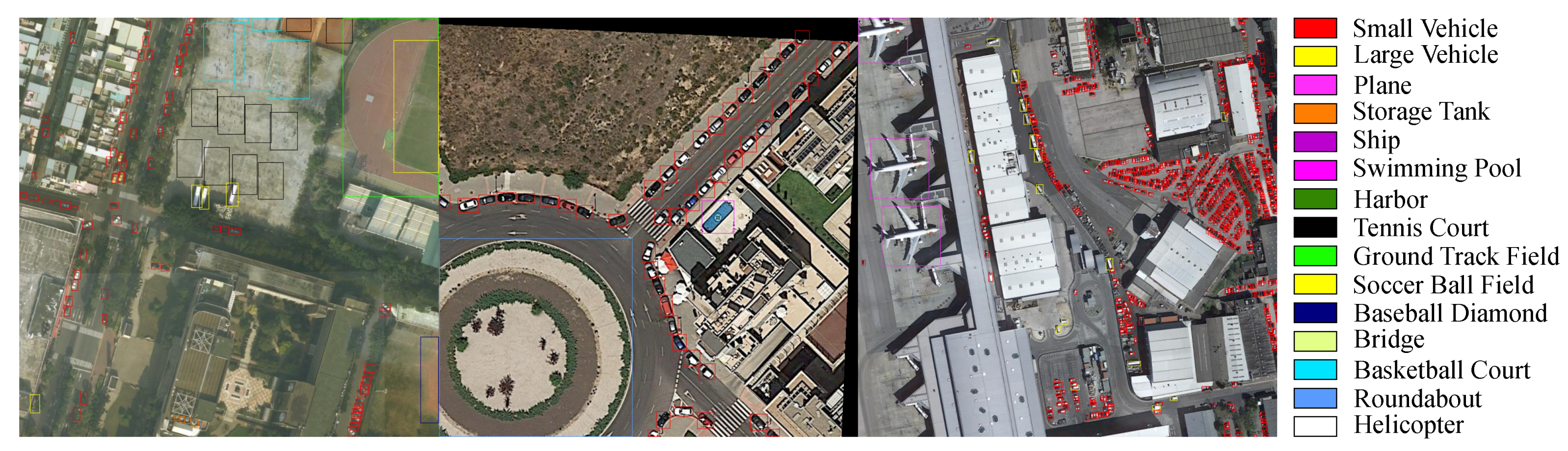


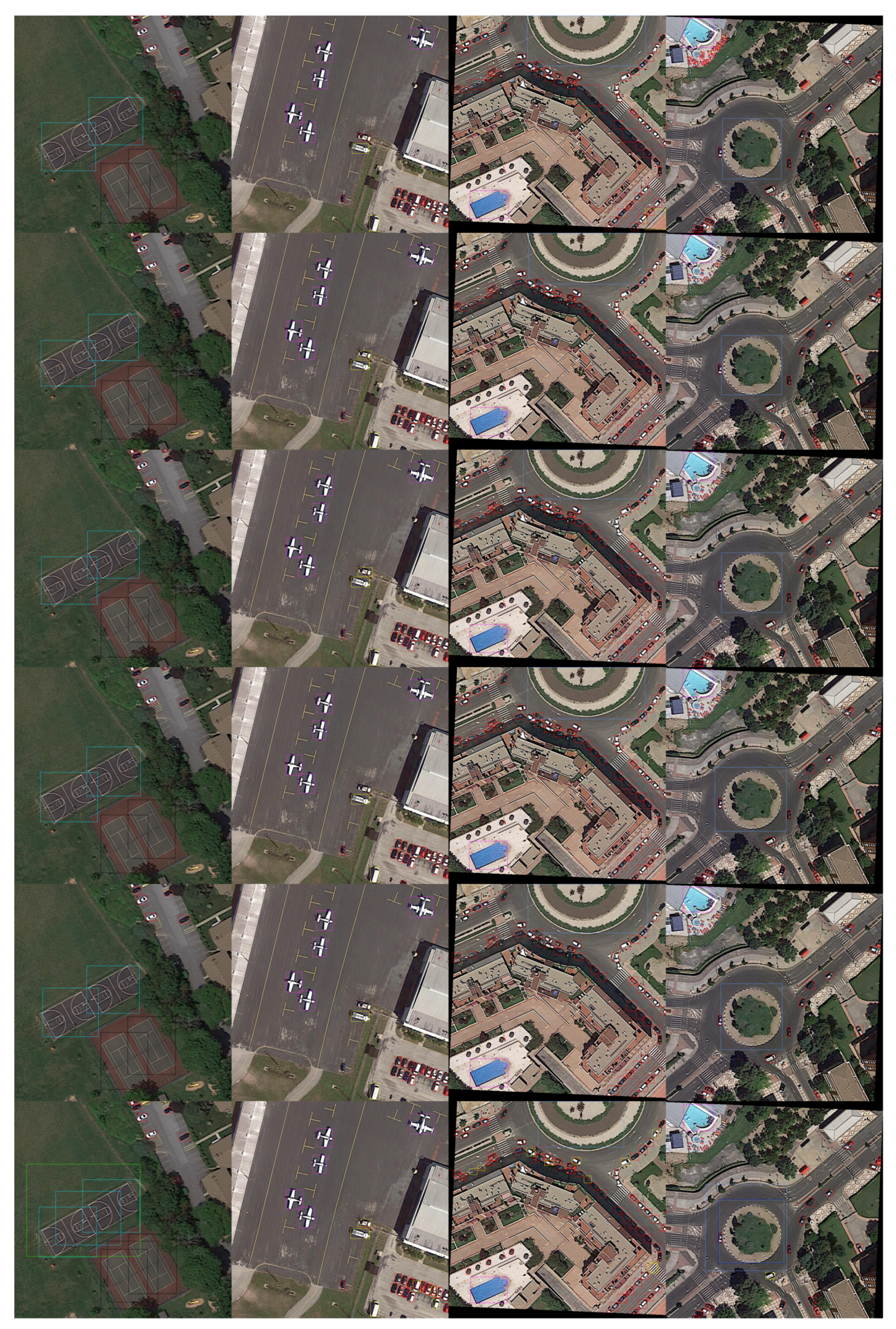

Publisher’s Note: MDPI stays neutral with regard to jurisdictional claims in published maps and institutional affiliations. |
© 2021 by the authors. Licensee MDPI, Basel, Switzerland. This article is an open access article distributed under the terms and conditions of the Creative Commons Attribution (CC BY) license (https://creativecommons.org/licenses/by/4.0/).