
Surface Urban Heat Islands Dynamics in Response to LULC and Vegetation across South Asia (2000–2019)


 , , and
Abstract
:
1. Introduction
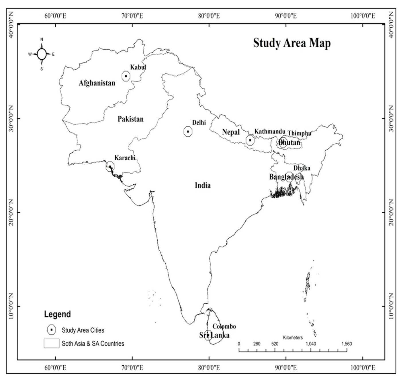
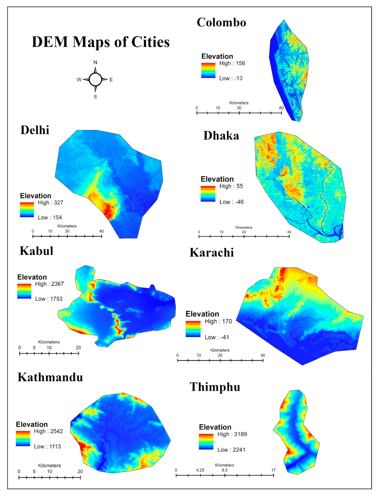
Study Area
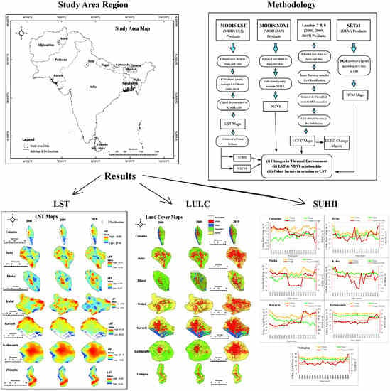
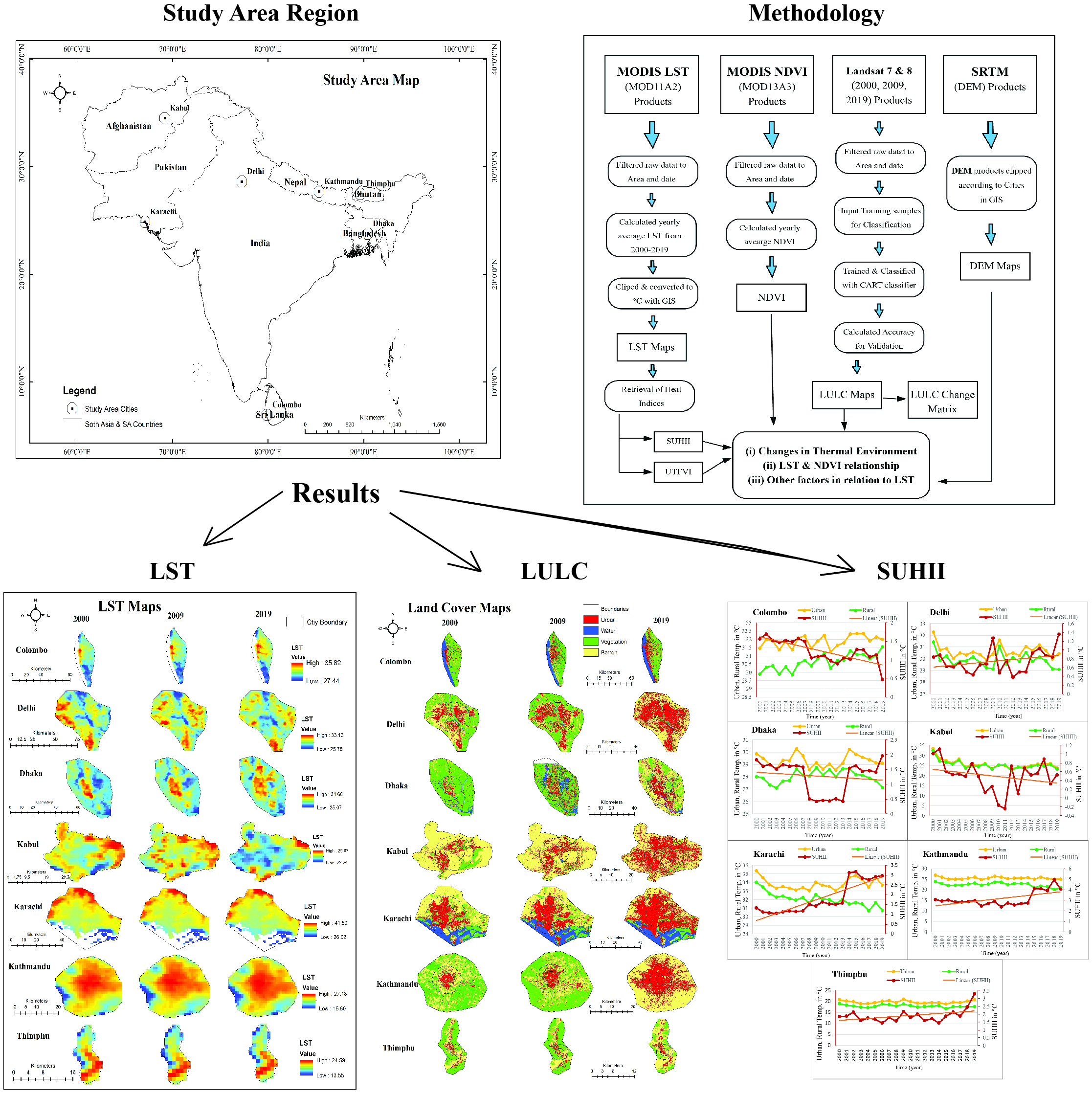
2. Materials and Methods
2.1. Datasets
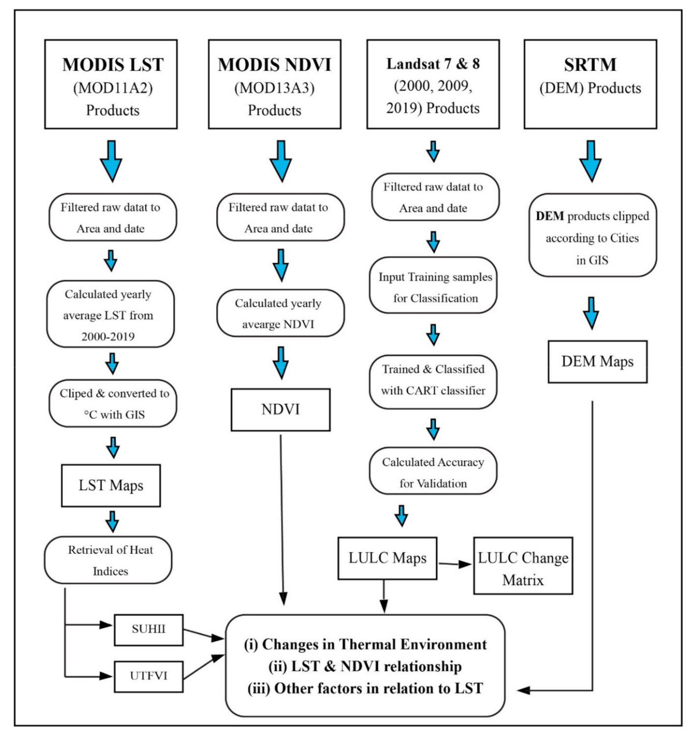
2.2. Methodology
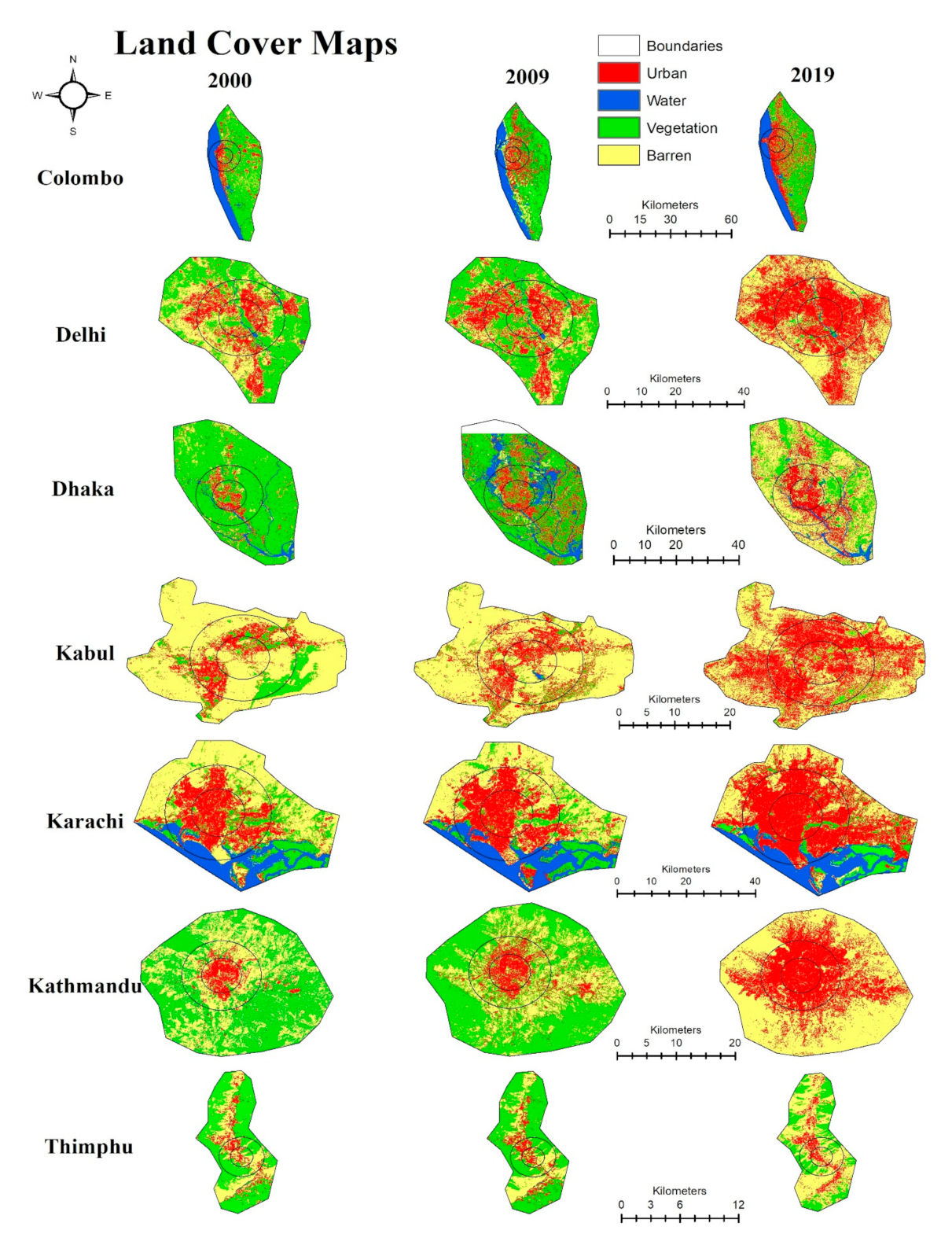
2.3. LULC Maps Preparation
2.4. Retrieval of Urban Heat Indices
2.4.1. Surface Urban Heat Island Intensity (SUHII)
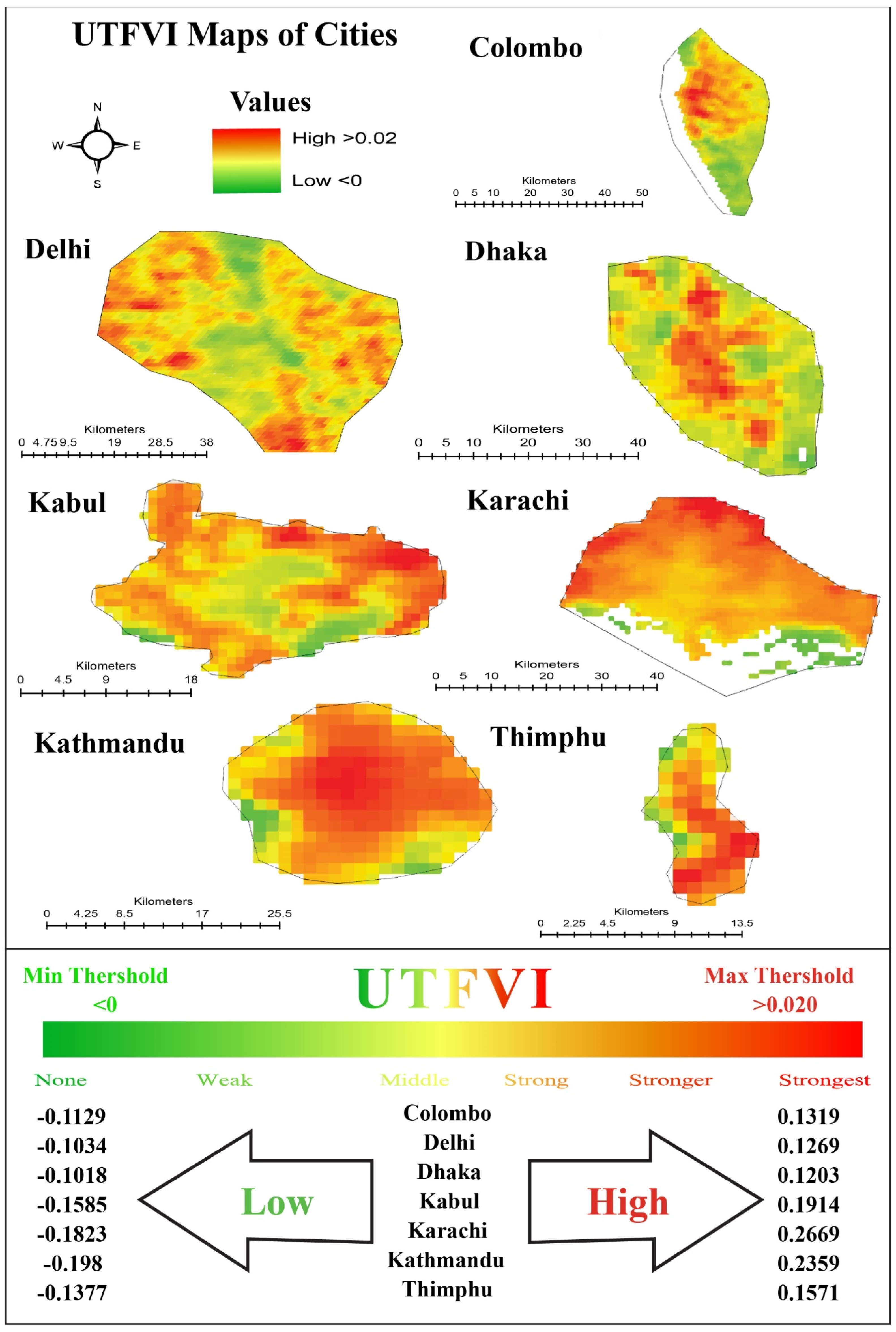
2.4.2. Urban Thermal Field Variance Index (UTFVI)
2.5. Statistical Analysis
3. Results
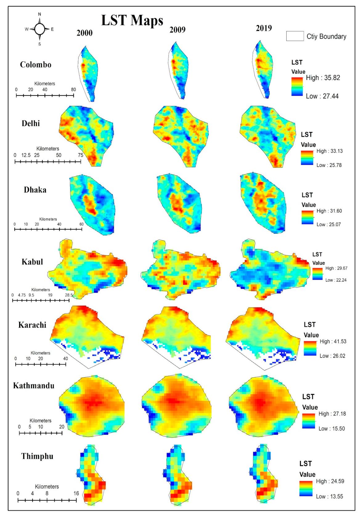
3.1. Spatial-Temporal Variations in LST (2000–2019)
3.2. Spatial-Temporal LULC Changes in SA Cities from 2000–2019
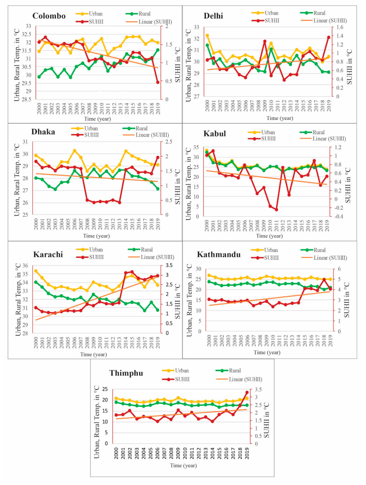
3.3. Surface Urban Heat Island Intensity (SUHII) Changes in Twenty Years
3.4. Changes in Urban Thermal Field Variance Index (UTFVI)
3.5. Role of Other Factors in UHI
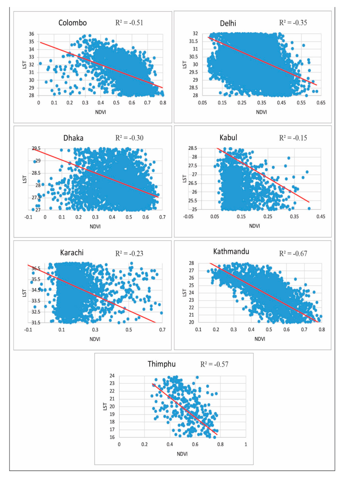
3.6. Statistical Analysis (Relationship between LST and NDVI
4. Discussion
Limitations and Future Research Directions
5. Conclusions
Author Contributions
Funding
Institutional Review Board Statement
Informed Consent Statement
Data Availability Statement
Acknowledgments
Conflicts of Interest
Abbreviations
| SUHI | Surface Urban Heat Island |
| GHG | Green House Gas |
| UHI | Urban Heat Island |
| IPCC | Intergovernmental Panel on Climate Change |
| LULC | Land Use Land Cover |
| LST | Land Surface Temperature |
| MODIS | Moderate Resolution Imaging Spectroradiometer |
| UTFVI | Urban Thermal Field Variance Index |
| NASA | National Aeronautics and Space Administration |
| SUHII | Surface Urban Heat Island Intensity |
| USGS | United States Geological Survey |
| NDVI | Normal Difference Vegetation Index |
| GEE | Google Earth Engine |
| CART | Classification And Regression Trees |
| SRTM | Shuttle Radar Topography Mission |
| CLHI | Canopy Layer Heat Island |
| DEM | Digital Elevation Model |
| BLHI | Boundary Layer Heat Island |
| UTE | Urban Thermal Environment |
| SHI | Surface Heat Island |
| UN | United Nations |
| UCL | Urban Canopy Layer |
| °C | Degree Celsius |
| OAQ | Outdoor Air Quality |
| °K | Degree Kelvin |
| RS | Remote Sensing |
| SPSS | Statistical Package for Social Sciences |
References
- Bureau, P.R. World Population Highlights: Key Findings from PRB’s 2007 World Population Data Sheet; Population Reference Bureau: Washington, DC, USA, 2007; Volume 62. [Google Scholar]
- Mirzaei, P.A.; Haghighat, F. Approaches to study urban heat island–abilities and limitations. Build. Environ. 2010, 45, 2192–2201. [Google Scholar] [CrossRef]
- Oke, T.R. The energetic basis of the urban heat island. Q. J. R. Meteorol. Soc. 1982, 108, 1–24. [Google Scholar] [CrossRef]
- Ana-Maria, B.; Mihai-Ionut, D.; Stelian, G.M.; Ștefana, B. Challenges regarding the study of urban heat islands. Rule set for researchers. In Proceedings of the Risk Reduction for Resilient Cities, Bucharest, Romania, 3–4 November 2016; p. 10. [Google Scholar]
- Shickman, K.; Alliance, G.C.C. Cool Policies for Cool Cities: Best Practices for Mitigating Urban Heat Islands in North American Cities. ACEEE Summer Study Energy Effic. Build. 2014, 1–53. [Google Scholar]
- Sarrat, C.; Lemonsu, A.; Masson, V.; Guedalia, D. Impact of urban heat island on regional atmospheric pollution. Atmos. Environ. 2006, 40, 1743–1758. [Google Scholar] [CrossRef]
- Landsberg, H.E. The Urban Climate; Academic Press: Cambridge, MA, USA, 1981. [Google Scholar]
- Ranagalage, M.; Estoque, R.C.; Handayani, H.H.; Zhang, X.; Morimoto, T.; Tadono, T.; Murayama, Y. Relation between urban volume and land surface temperature: A comparative study of planned and traditional cities in Japan. Sustainability 2018, 10, 2366. [Google Scholar] [CrossRef] [Green Version]
- Wang, R.; Derdouri, A.; Murayama, Y. Spatiotemporal simulation of future land use/cover change scenarios in the Tokyo metropolitan area. Sustainability 2018, 10, 2056. [Google Scholar] [CrossRef] [Green Version]
- Rousta, I.; Sarif, M.O.; Gupta, R.D.; Olafsson, H.; Ranagalage, M.; Murayama, Y.; Zhang, H.; Mushore, T.D. Spatiotemporal analysis of land use/land cover and its effects on surface urban heat island using Landsat data: A case study of Metropolitan City Tehran (1988–2018). Sustainability 2018, 10, 4433. [Google Scholar] [CrossRef] [Green Version]
- Troude, F.; Dupont, E.; Carissimo, B.; Flossmann, A.I. Relative influence of urban and orographic effects for low wind conditions in the Paris area. Bound. Layer Meteorol. 2002, 103, 493–505. [Google Scholar] [CrossRef]
- Tso, C. A survey of urban heat island studies in two tropical cities. Atmos. Environ. 1996, 30, 507–519. [Google Scholar] [CrossRef]
- Hirano, Y.; Fujita, T. Evaluation of the impact of the urban heat island on residential and commercial energy consumption in Tokyo. Energy 2012, 37, 371–383. [Google Scholar] [CrossRef]
- Streutker, D.R. A remote sensing study of the urban heat island of Houston, Texas. Int. J. Remote Sens. 2002, 23, 2595–2608. [Google Scholar] [CrossRef]
- Kim, H.H. Urban heat island. Int. J. Remote Sens. 1992, 13, 2319–2336. [Google Scholar] [CrossRef]
- Camilloni, I.; Barros, V. On the urban heat island effect dependence on temperature trends. Clim. Chang. 1997, 37, 665–681. [Google Scholar] [CrossRef]
- Li, Q.; Zhang, H.; Liu, X.; Huang, J. Urban heat island effect on annual mean temperature during the last 50 years in China. Theor. Appl. Climatol. 2004, 79, 165–174. [Google Scholar] [CrossRef]
- Kim, Y.-H.; Baik, J.-J. Daily maximum urban heat island intensity in large cities of Korea. Theor. Appl. Climatol. 2004, 79, 151–164. [Google Scholar] [CrossRef]
- Zhang, P.; Imhoff, M.L.; Bounoua, L.; Wolfe, R.E. Exploring the influence of impervious surface density and shape on urban heat islands in the northeast United States using MODIS and Landsat. Can. J. Remote Sens. 2012, 38, 441–451. [Google Scholar]
- Bokaie, M.; Zarkesh, M.K.; Arasteh, P.D.; Hosseini, A. Assessment of urban heat island based on the relationship between land surface temperature and land use/land cover in Tehran. Sustain. Cities Soc. 2016, 23, 94–104. [Google Scholar] [CrossRef]
- Estoque, R.C.; Murayama, Y.; Myint, S.W. Effects of landscape composition and pattern on land surface temperature: An urban heat island study in the megacities of Southeast Asia. Sci. Total Environ. 2017, 577, 349–359. [Google Scholar] [CrossRef]
- Ranagalage, M.; Estoque, R.C.; Murayama, Y. An urban heat island study of the Colombo metropolitan area, Sri Lanka, based on Landsat data (1997–2017). ISPRS Int. J. Geo-Inf. 2017, 6, 189. [Google Scholar] [CrossRef] [Green Version]
- Babazadeh, M.; Kumar, P. Estimation of the urban heat island in local climate change and vulnerability assessment for air quality in Delhi. Eur. Sci. J. 2015, 19, 55–65. [Google Scholar]
- Ellis, P.; Roberts, M. Leveraging Urbanization in South Asia: Managing Spatial Transformation for Prosperity and Livability; The World Bank: Washington, DC, USA, 2016; Volume 10, pp. 971–978. [Google Scholar]
- Cohen, B. Urbanization, City growth, and the New United Nations development agenda. Cornerstone 2015, 3, 4–7. [Google Scholar]
- Kotharkar, R.; Ramesh, A.; Bagade, A. Urban heat island studies in South Asia: A critical review. Urban Clim. 2018, 24, 1011–1026. [Google Scholar] [CrossRef]
- Karekezi, S.; McDade, S.; Boardman, B.; Kimani, J. Energy, poverty, and development. In Global Energy Assessment–Toward a Sustainable Future; Cambridge University Press: Cambridge, UK, 2012; pp. 151–190. [Google Scholar]
- Sumner, A.; Suryahadi, A.; Thang, N. Poverty and Inequalities in Middle-Income Southeast Asia; Institute of Development Studies (IDS): Brighton, UK, 2012. [Google Scholar]
- The World Bank. Trends in Greenhouse Gas Emissions. 2017. Available online: wdi.worldbank.org/table/3.9 (accessed on 12 May 2020).
- WHO. WHO Global Urban Ambient Air Pollution Database (Update 2016); WHO: Geneva, Switzerland, 2016. [Google Scholar]
- Lahiri-Dutt, K. Energy Resources in South Asia: The Last Frontier? 2003. Available online: researchgate.net (accessed on 10 May 2020).
- Alexander, L.V. Global observed long-term changes in temperature and precipitation extremes: A review of progress and limitations in IPCC assessments and beyond. Weather Clim. Extre. 2016, 11, 4–16. [Google Scholar]
- Li, X.X.; Koh, T.Y.; Entekhabi, D.; Roth, M.; Panda, J.; Norford, L.K. A multi-resolution ensemble study of a tropical urban environment and its interactions with the background regional atmosphere. J. Geophys. Res. Atmos. 2013, 118, 9804–9818. [Google Scholar] [CrossRef]
- Roth, M.; Oke, T.; Emery, W. Satellite-derived urban heat islands from three coastal cities and the utilization of such data in urban climatology. Int. J. Remote Sens. 1989, 10, 1699–1720. [Google Scholar] [CrossRef]
- Oke, T.R. City size and the urban heat island. Atmos. Environ. 1973, 7, 769–779. [Google Scholar] [CrossRef]
- Shashua-Bar, L.; Pearlmutter, D.; Erell, E. The influence of trees and grass on outdoor thermal comfort in a hot-arid environment. Int. J. Climatol. 2011, 31, 1498–1506. [Google Scholar] [CrossRef]
- Arnfield, A.J. Two decades of urban climate research: A review of turbulence, exchanges of energy and water, and the urban heat island. Int. J. Climatol. J. R. Meteorol. Soc. 2003, 23, 1–26. [Google Scholar] [CrossRef]
- Billah, M. South Asian Association for Regional Co-operation & its Contribution to the South Asian Politics and Economy. Int. J. Empirical Educ. Res. 2019, 3, 21–30. [Google Scholar]
- Ramakrishnan, P.; Rao, K.; Chandrashekara, U.; Chhetri, N.; Gupta, H.; Patnaik, S.; Saxena, K.; Sharma, E. South Asia. In Traditional Forest-Related Knowledge; Springer: Berlin, Germany, 2012; pp. 315–356. [Google Scholar]
- Mwaniki, D. Regional Training Workshop on Human Settlement Indicators, Global City Definition. 2018. UN Habitat, United Nations Escap. Available online: unescap.org/sites/default/files/6.Working_definition_of_a_city_for_SDG11_UN-Habitat_Wshop_26-29Mar2018.pdf (accessed on 8 July 2021).
- Bank, W. How Do We Define Cities, Towns, and Rural Areas? 2020. Available online: blogs.worldbank.org (accessed on 8 July 2021).
- Dick, H.W.; Rimmer, P.J. Beyond the third world city: The new urban geography of South-east Asia. Urban Stud. 1998, 35, 2303–2321. [Google Scholar] [CrossRef]
- City Population. Available online: worldpopulationreview.com (accessed on 5 May 2020).
- Mutanga, O.; Kumar, L. Google Earth Engine Applications. Remote Sens. 2019, 11, 591. [Google Scholar] [CrossRef] [Green Version]
- Foundation, N.S. OpenTopography High-Resolution Topography Data and Tools. Available online: opentopography.org (accessed on 16 May 2020).
- Brownlee, J. Classification and regression trees for machine learning. Mach. Learn. Algorithms 2016. Available online: http://machinelearningmastery.com/classification-and-regression-trees-for-machine-learning (accessed on 8 March 2020).
- Qian, Y.; Zhou, W.; Yan, J.; Li, W.; Han, L. Comparing machine learning classifiers for object-based land cover classification using very high resolution imagery. Remote Sens. 2015, 7, 153–168. [Google Scholar] [CrossRef]
- Zhang, K.; Wang, R.; Shen, C.; Da, L. Temporal and spatial characteristics of the urban heat island during rapid urbanization in Shanghai, China. Env. Monit Assess 2010, 169, 101–112. [Google Scholar] [CrossRef]
- Liu, L.; Zhang, Y. Urban heat island analysis using the Landsat TM data and ASTER data: A case study in Hong Kong. Remote Sens. 2011, 3, 1535–1552. [Google Scholar] [CrossRef] [Green Version]
- Zhang, Y.; Yu, T.; Gu, X. Land surface temperature retrieval from cbers-02 irmss thermal infrared data and its applications in quantitative analysis of urban heat island effect. J. Remote Sens. 2001, 1, 789–803. [Google Scholar]
- Simwanda, M.; Ranagalage, M.; Estoque, R.C.; Murayama, Y. Spatial analysis of surface urban heat islands in four rapidly growing African cities. Remote Sens. 2019, 11, 1645. [Google Scholar] [CrossRef] [Green Version]
- Chung, Y.-S.; Yoon, M.-B.; Kim, H.-S. On climate variations and changes observed in South Korea. Clim. Chang. 2004, 66, 151–161. [Google Scholar] [CrossRef]
- Liu, W.; Ji, C.; Zhong, J.; Jiang, X.; Zheng, Z. Temporal characteristics of the Beijing urban heat island. Theor. Appl. Climatol. 2007, 87, 213–221. [Google Scholar] [CrossRef]
- Lu, L.; Guo, H.; Corbane, C.; Li, Q. Urban sprawl in provincial capital cities in China: Evidence from multi-temporal urban land products using Landsat data. Sci. Bull 2019, 64, 955–957. [Google Scholar] [CrossRef] [Green Version]
- Fu, P.; Weng, Q. Variability in annual temperature cycle in the urban areas of the United States as revealed by MODIS imagery. ISPRS J. Photogramm. Remote Sens. 2018, 146, 65–73. [Google Scholar] [CrossRef]
- Renard, F.; Alonso, L.; Fitts, Y.; Hadjiosif, A.; Comby, J. Evaluation of the effect of urban redevelopment on surface urban heat islands. Remote Sens. 2019, 11, 299. [Google Scholar] [CrossRef] [Green Version]
- He, C.; Shi, P.; Xie, D.; Zhao, Y. Improving the normalized difference built-up index to map urban built-up areas using a semiautomatic segmentation approach. Remote Sens. Lett. 2010, 1, 213–221. [Google Scholar] [CrossRef] [Green Version]
- Tran, H.; Uchihama, D.; Ochi, S.; Yasuoka, Y. Assessment with satellite data of the urban heat island effects in Asian mega cities. Int. J. Appl. Earth Obs. Geoinf. 2006, 8, 34–48. [Google Scholar] [CrossRef]
- Weng, Q.; Lu, D.; Schubring, J. Estimation of land surface temperature–vegetation abundance relationship for urban heat island studies. Remote Sens. Environ. 2004, 89, 467–483. [Google Scholar] [CrossRef]
- Zareie, S.; Khosravi, H.; Nasiri, A.; Dastorani, M. Using Landsat Thematic Mapper (TM) sensor to detect change in land surface temperature in relation to land use change in Yazd, Iran. Solid Earth 2016, 7, 1551–1564. [Google Scholar] [CrossRef] [Green Version]
- Dilawar, A.; Chen, B.; Trisurat, Y.; Tuankrua, V.; Arshad, A.; Hussain, Y.; Measho, S.; Guo, L.; Kayiranga, A.; Zhang, H. Spatiotemporal shifts in thermal climate in responses to urban cover changes: A-case analysis of major cities in Punjab, Pakistan. Geomat. Nat. Hazards Risk 2021, 12, 763–793. [Google Scholar] [CrossRef]
- Rehan, R.M. Cool city as a sustainable example of heat island management case study of the coolest city in the world. HBRC J. 2016, 12, 191–204. [Google Scholar] [CrossRef] [Green Version]
- Meinhold, B. A super futuristic net zero high speed rail station for Stuttgart. Inhabitat 2010. Available online: inhabitat.com (accessed on 15 August 2020).
- Mell, I. GLOBAL Green Infrastructure: Lessons for Successful Policy-Making, Investment and Management; Taylor & Francis Group: London, UK, 2016. [Google Scholar]
- O’Malley, C.; Piroozfar, P.; Farr, E.R.; Pomponi, F. Urban Heat Island (UHI) mitigating strategies: A case-based comparative analysis. Sustain. Cities Soc. 2015, 19, 222–235. [Google Scholar] [CrossRef] [Green Version]


| No. | Countries of SA | Megacities/Largest | Area (km2) | Population (year) | Elevation (m) | Geography/Landform |
|---|---|---|---|---|---|---|
| 1. | Afghanistan | Kabul | 275 | 4,434,550 (2020) | 1790 | Mountain Valley |
| 2. | Bangladesh | Dhaka | 306.4 | 14,543,124 (2011) | 9 | Plain Area |
| 3. | Bhutan | Thimphu | 26.1 | 146,500 (2019) | 2300 | Mountain Valley |
| 4. | India | Delhi | 1484 | 16,787,941 (2011) | 215 | Plain Area |
| 5. | Nepal | Kathmandu | 51 | 1,003,285 (2011) | 1336 | Mountain Valley |
| 6. | Pakistan | Karachi | 3780 | 16,054,988 (2017) | 21 | Coastal Plain |
| 7. | Sri-Lanka | Colombo | 37.31 | 2,324,349 (2012) | 4 | Coastal Plain |
| Urban Thermal Field Variance Index Threshold | Urban Heat Island Phenomenon | Ecological Conditions Evaluation |
|---|---|---|
| <0 | None | Excellent |
| 0.000–0.005 | Weak | Good |
| 0.005–0.010 | Middle | Normal |
| 0.010–0.015 | Strong | Bad |
| 0.015–0.020 | Stronger | Worse |
| >0.020 | Strongest | Worst |
| No. | Classified SA Cities | Overall Accuracy 2000 | Overall Accuracy 2009 | Overall Accuracy 2019 |
|---|---|---|---|---|
| 1 | Colombo | 80 % | 83 % | 90 % |
| 2 | Delhi | 79% | 82 % | 91 % |
| 3 | Dhaka | 78 % | 83 % | 88 % |
| 4 | Kabul | 77 % | 82 % | 86 % |
| 5 | Karachi | 79 % | 86 % | 88 % |
| 6 | Kathmandu | 81 % | 85 % | 91 % |
| 7 | Thimphu | 78 % | 81 % | 87 % |
| Cities | LC Type | 2000 | 2009 | 2019 | Transferred Area |
|---|---|---|---|---|---|
| Colombo | Urban | 6.32 | 8.1 | 13.75 | 7.43 |
| Water | 13.48 | 13.64 | 12.99 | −0.49 | |
| Vegetation | 11.78 | 12.69 | 9.34 | −2.44 | |
| Barren | 4.68 | 6.27 | 5.36 | 0.68 | |
| Delhi | Urban | 145.63 | 273.74 | 631.01 | 485.38 |
| Water | 28.01 | 30.66 | 26.31 | −1.7 | |
| Vegetation | 921.4 | 1056.59 | 744.23 | −177.17 | |
| Barren | 93.26 | 101.95 | 123.51 | 30.25 | |
| Dhaka | Urban | 90.03 | 127.27 | 188.16 | 98.13 |
| Water | 66.83 | 80.98 | 54.53 | −12.3 | |
| Vegetation | 181.33 | 161.66 | 145.99 | −35.34 | |
| Barren | 18.54 | 11.79 | 10.84 | −7.7 | |
| Kabul | Urban | 112.23 | 195.68 | 229.81 | 117.58 |
| Water | 1.73 | 1.99 | 0.14 | −1.59 | |
| Vegetation | 282.4 | 357.9 | 197.52 | −84.88 | |
| Barren | 16.55 | 18.34 | 18.9 | 2.35 | |
| Karachi | Urban | 164.27 | 256.46 | 397.17 | 232.9 |
| Water | 96.47 | 163.97 | 159.01 | 62.54 | |
| Vegetation | 102.33 | 91.76 | 82.91 | −19.42 | |
| Barren | 114.73 | 143.6 | 164.91 | 50.18 | |
| Kathmandu | Urban | 5.6 | 17.82 | 35.21 | 29.61 |
| Water | 0.49 | 0.29 | 0.47 | −0.02 | |
| Vegetation | 41.75 | 62.16 | 36.35 | −5.4 | |
| Barren | 53.81 | 29.18 | 14.89 | −38.92 | |
| Thimphu | Urban | 4.94 | 5.57 | 7.46 | 2.52 |
| Water | 0.34 | 0.39 | 0.81 | 0.47 | |
| Vegetation | 19.21 | 21.68 | 16.63 | −2.58 | |
| Barren | 3.79 | 2.97 | 4.5 | 0.71 |
| Cities | Radius of Urban Buffer (km) | Radius of Rural Buffer (km) | Koppen-Gelger Zone Classification |
|---|---|---|---|
| Colombo | 4 | 8 | “Af” (Tropical Rainforest Climate) |
| Delhi | 8 | 16 | “Cfa” (Humid Subtropical Climate) |
| Dhaka | 5 | 10 | “Aw” (Tropical Savanna Climate) |
| Kabul | 4 | 8 | “Dfb” (Warm Summer Continental Climate) |
| Karachi | 7 | 14 | “Bwh” (Tropical and Subtropical Desert Climate) |
| Kathmandu | 3 | 6 | “Cfa” (Humid Subtropical Climate) |
| Thimphu | 1 | 2 | “ET” (Tundra Climate) |
Publisher’s Note: MDPI stays neutral with regard to jurisdictional claims in published maps and institutional affiliations. |
© 2021 by the authors. Licensee MDPI, Basel, Switzerland. This article is an open access article distributed under the terms and conditions of the Creative Commons Attribution (CC BY) license (https://creativecommons.org/licenses/by/4.0/).
Share and Cite
Hassan, T.; Zhang, J.; Prodhan, F.A.; Pangali Sharma, T.P.; Bashir, B. Surface Urban Heat Islands Dynamics in Response to LULC and Vegetation across South Asia (2000–2019). Remote Sens. 2021, 13, 3177. https://doi.org/10.3390/rs13163177
Hassan T, Zhang J, Prodhan FA, Pangali Sharma TP, Bashir B. Surface Urban Heat Islands Dynamics in Response to LULC and Vegetation across South Asia (2000–2019). Remote Sensing. 2021; 13(16):3177. https://doi.org/10.3390/rs13163177
Chicago/Turabian StyleHassan, Talha, Jiahua Zhang, Foyez Ahmed Prodhan, Til Prasad Pangali Sharma, and Barjeece Bashir. 2021. "Surface Urban Heat Islands Dynamics in Response to LULC and Vegetation across South Asia (2000–2019)" Remote Sensing 13, no. 16: 3177. https://doi.org/10.3390/rs13163177
APA StyleHassan, T., Zhang, J., Prodhan, F. A., Pangali Sharma, T. P., & Bashir, B. (2021). Surface Urban Heat Islands Dynamics in Response to LULC and Vegetation across South Asia (2000–2019). Remote Sensing, 13(16), 3177. https://doi.org/10.3390/rs13163177