Abstract
Estimating the potential achievable solar energy in urban buildings is significantly important for the long-term planning and development of environmental protection strategies. Nevertheless, conventional methods based on LiDAR data are often costly and require more than one platform to obtain complete building surface information. The development of oblique photogrammetry technology enables fast and accurate acquiring of the 3D information of the surface. In this paper, we propose an efficient method to estimate the potential achievable solar energy of building surfaces based on photogrammetric mesh models. In this method, we use photogrammetric mesh models as the input data and then propose a hierarchical algorithm for shadow analysis. Combined with the solar radiation model, we then obtain the potential achievable solar energy of the building surface. We further investigate the performance of the proposed method and it is shown that this method outperforms the multi-source LiDAR data.
1. Introduction
The population growth expands the urban areas resulting in increased energy consumption. The proven reserves of coal, oil, and natural gas are however unable to meet the needs of human development hence there is an immediate need for further production of renewable energy. Solar energy is clean and pollution-free renewable energy and is considered one of the main alternatives to traditional energy sources. Solar energy is widely produced through solar cells installed on the roof of buildings especially in areas with abundant sunlight [1]. Nevertheless, the urban buildings in densely populated areas are often extended vertically. This results in shielding of the building surfaces resulting in uneven distribution of potential achievable solar energy. Estimating the potential achievable solar energy of the buildings can effectively reduce the cost of solar energy production and further extend the scale of solar energy utilization.
In recent years, light detection and ranging (LiDAR) data have been widely applied in assessing the potential achievable solar energy due to their robustness in identifying the buildings’ orientations and the slope of their roof planes [2]. In 2005, Voegtle et al. proposed using airborne laser scanning (ALS) data for the determination of suitable areas for installing photovoltaic cells [3]. Their research suggests that the ALS data can be used to estimate the area and slope of the roofs and help to select suitable areas for installing photovoltaic cells. Their method is however unable to estimate the actual potential achievable solar energy. Soon after, Yu et al. (2009) attempted using LiDAR data to produce a digital surface model (DSM) to analyze the variations of solar radiation in urban environments [4]. Hofierka et al. also proposed a method for the assessment of photovoltaic potential in urban areas using open-source solar radiation tools [5].
The above-mentioned earlier research works proposed techniques to estimate the potential achievable solar energy of the roof surfaces, however, they did not incorporate the impact of other objects on solar energy production. In 2013, Redweik et al. developed a shading algorithm to consider the influence of shadows on the potential achievable solar energy of buildings [6]. However, the reduction from a 3D point cloud into a 2.5D raster-based model will reduce the details and accuracy for further analysis. In many subsequent studies, LiDAR data were used as the primary data to select suitable photovoltaic areas, and then the shadow was added to improve the accuracy of the corresponding estimations. For instance, [2,7,8,9,10,11] modeled each roof structure separately and focused on the potential solar energy of the building roof without considering the potential solar energy of the facades.
With the continuous vertical extension of the urban areas, the height of the buildings is also increased. This enables the deployment of photovoltaic cells on the building facade. Several previous works also proposed techniques to assess the potential achievable solar energy of the vertical walls. For example, Lee et al. (2009) used LiDAR and GIS data to interpolate the city’s DSM and estimate the solar radiation availability on the roofs and facades [12]. Redweik et al. (2013) also estimated the solar potential of building facades by using DSM data [6]. There are also similar research works in [13,14,15,16]. Using DSM to analyze the solar potential of facades, however, is based on extruding the roof outlines to the ground for obtaining an abstract faced model. Such models however ignore the details of the building’s facade hence there may be discrepancies between the estimated results and actual measurements.
Note that terrestrial laser scanning (TLS) can obtain more details from the vertical walls than the ALS data. Therefore, TLS data are often employed to assess the potential achievable solar energy of the vertical walls. For example, Jochem et al. (2011) proposed a method for automatic solar radiation modeling of the facades acquired by mobile laser scanning (MLS) data [17]. They extracted facades from the MLS data and obtained the details of the building facades. In 2017, Huang et al. (2017) also used TLS data to extract the regions of interest and simulated solar radiation of the targeted scene for a given period [18]. Liang et al. (2018) proposed a method based on multi-source point clouds, taking into account the shading of surrounding buildings for solar energy potential estimation of building facades [19]. Although TLS and MLS can accurately obtain detailed information of the buildings’ facades and retain high-resolution geometric information, it is difficult to obtain building roof information at the same time [20,21]. This limits their applicability in assessing the potential achievable solar energy of buildings.
It is also concluded in [22] that in assessing potential achievable solar energy there is an immediate need and emerging trend for shifting away from simple 2D visualization to more complex 3D representation and analysis. Both LiDAR data and photogrammetric mesh models (three-dimensional models generated from airborne oblique photogrammetry) can obtain 3D information of the urban areas. However, obtaining complete facade and roof information from LiDAR data requires the fusion of ground-based and airborne LiDAR which is rather time-consuming and expensive. Along with the development of the multi-view stereo matching method and aerial oblique photogrammetric system, oblique photogrammetry has emerged as a popular method to obtain building models [23,24,25]. It can obtain detailed information of the buildings’ roofs and facades and is less expensive than LiDAR data. The accuracy of the 3D model obtained from oblique photogrammetry can also reach within 5 cm [26,27]. These motivate the exploration of the photogrammetric mesh models to estimate potential achievable solar energy of the urban buildings [28].
Shadow analysis is essential for estimating potential achievable solar energy of the buildings based on the DSM of the 3D regular model. Shadow projection algorithms are often used for shadow analysis in assessing the potential achievable solar energy using DSM data [14,29]. These algorithms determine whether a given point is located in the shadow by checking whether there is an occlusion between the surface points and the light source. The current shadow analysis methods are developed for regular DSM data derived from LiDAR or photogrammetry, hence they cannot be directly adapted to the photogrammetric mesh models. In addition to the above approaches, some shadow analysis algorithms are directly performed on the point clouds. The shadow analysis method in Jochem’s work takes the detection point as the center and then subdivides the horizontal plane into fan-shaped areas with given intervals. The part that contains the current azimuth of the sun is then recognized and the highest point of this part is obtained to determine whether it is higher than the sun’s elevation angle [17,30]. Further, in Vo’s work, a new shadow analysis method is developed that rotates the original coordinate axis Z of the area of interest to make it parallel to the sun’s ray direction vector. Then the rotating point cloud is discretized into areas of the same size on the XY plane. The point cloud in each cell is then classified into different clusters using Density-Based Spatial Clustering of Applications with Noise (BSCAN) clustering algorithm and the top-most point cloud is assigned as the illuminated point [31]. Nevertheless, this method has strict requirements for the even distribution of the point cloud data hence cannot be directly used on photogrammetric mesh models. The efficiency of the DBSCAN clustering algorithm is also not easy to control.
Inspired by the work of Vo, we propose a hierarchical shadow analysis method for the photogrammetric mesh models, which is presented in Section 2. In Section 3 we then present the experimental results. We then compare the solar irradiance results calculated by the proposed method with those obtained by the ArcGIS and LiDAR data. The solar energy distributions on the facade and roof are also analyzed for different time scales. Finally, in Section 4, we summarize this work and draw our research conclusions.
2. Method
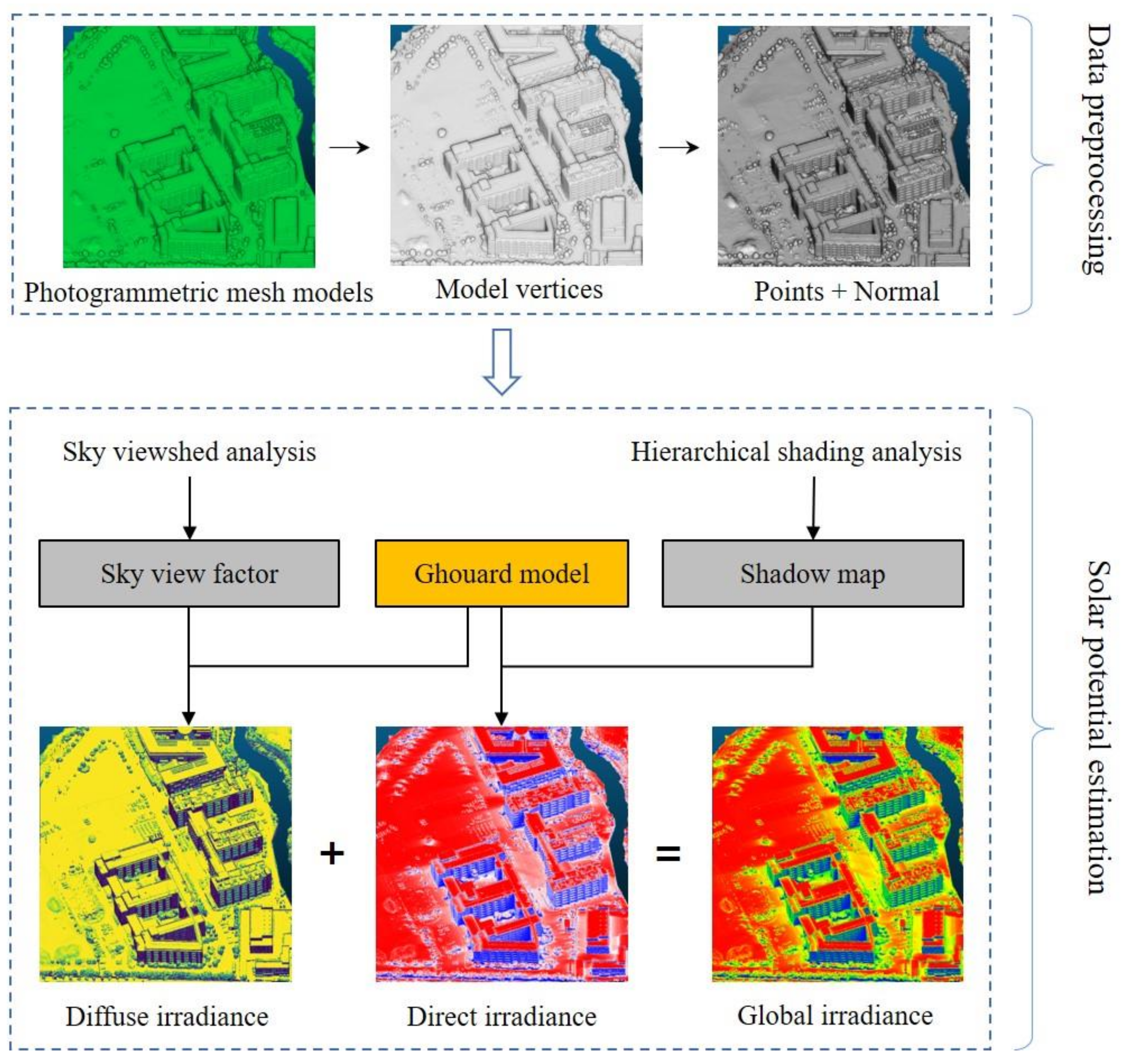
This paper aims to estimate the potential solar energy of facades and roofs based on the photogrammetric mesh models. The proposed method is comprised of two main steps as shown in Figure 1. The details of these steps are presented as follows.

Figure 1.
The flowchart of the proposed method.
2.1. Point Cloud Feature Computing
The original data used in this paper include photogrammetric mesh models established from the oblique images collected through a UAV. The camera mounted on the UAV can obtain both the top and side information of the ground objects. Consequently, the 3D models created by oblique images were truly reflective of the object’s appearance, location, height, and other attributes. It can provide reliable data for the solar energy potential assessment process.
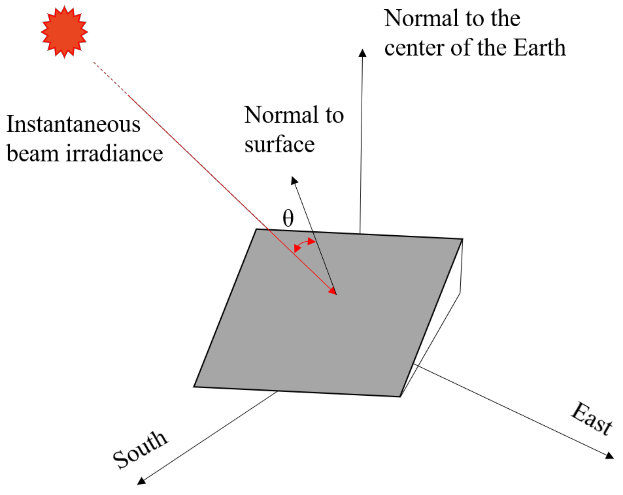
As illustrated in Figure 2, θ is the angle between the solar irradiance on the inclined plane and the instantaneous beam irradiance. To quantify the solar irradiance received on an inclined plane along the normal, the normal vector of the local surface at the illuminated point must be calculated. We used the Hough transform method to calculate the normal vectors at the vertices of the 3D model. This is because the method of calculating the normal vectors at the vertices of the 3D model based on the Hough transform method is robust in dealing with the noise points and outliers [32]. For each vertex, several nearby points was used to fit a plane, then the normal of the plane was set to each vertex for convenient subsequent processing. This method has been also integrated into the open-source software CloudCompare, and its calculation details are available at https://github.com/cloudcompare/cloudcompare (accessed on 1 May 2021).
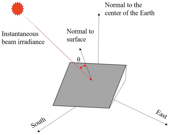
Figure 2.
Relationship between the normal of the face and the instantaneous beam irradiance.
2.2. Solar Potential Estimation
The total solar radiation GTh received on the surface of the building can be divided into direct radiation BTh and diffuse radiation DTh as in Equation (1) adopted from Brito [33]. Direct radiation is the received energy upon the direct impact of the sun’s rays on the surface of an object which accounts for the main part of the total solar radiation. Most of the existing solar radiation models accurately calculate the direct component per hour. The calculation of the scattering component is however a complex task. It is more difficult to calculate diffuse radiation compared with direct radiation. This is because diffuse radiation has many forms, including isotropic diffuse, circumsolar diffuse, and horizon brightening [34,35]. Different solar radiation models are chosen to calculate the solar irradiance of the buildings’ surfaces, and there may be some deviation in the results. By comparing different solar radiation models, Mghouchi found that the solar irradiance calculated by the Ghouard model is the closest to the actual measured value [36]. Therefore, in this paper, the Ghouard solar radiation model was chosen to calculate the solar irradiance on the building surface.
where BTh and DTh represent the instantaneous direct and diffuse irradiance on the inclined plane, vis denotes the shadow analysis result (which is either 0 or 1), and SVF denotes the sky view factor result. In the following, we elaborate on the calculation of these four values.
2.2.1. Direct Irradiance
As seen in Equation (1), we need to obtain the direct and diffuse radiation components. The cumulative direct radiation on the inclined surface was obtained using Equation (2). The cumulative direct radiation received on the inclined surface in a day is the integral of the instantaneous direct radiation from sunrise to sunset. To simplify the calculation process of this definite integral, the idea of partition was adopted in the actual calculation process, that is, the product of the average value of instantaneous direct radiation in a period and the length of the period. Kumar et al. suggested using 30 min as an appropriate time interval to ensure computational efficiency and accuracy [37].
where trs and tss denote sunrise and sunset times, respectively. θ is the angle between the sun’s rays and the normal of the inclined plane, β is the sun elevation angle, which is determined by local latitude and time [37]. In Equation (2), Gbh is the instantaneous beam irradiance on the horizontal plane, which is only affected by the sun elevation angle β, atmospheric transmittance, and altitude [36]. The value of Gbh is obtained using the Ghouard model [6]:
where = 1367 W/m2, , n represents the day of the year, ranging from 1 in January to 365 or 366 on the 31 December, and are the coefficients of the turbidity factor as given in Table 1:

Table 1.
The turbidity factors.
Due to the obstruction of the surrounding environment and the change of the incident angle of the sun’s rays, some locations might not be able to receive direct sunlight. Therefore, the actual direct radiation received on the inclined surface needs to be multiplied by the shadow analysis result, vis.
2.2.2. Diffuse Irradiance
In the existing research works, several models have been provided for diffuse radiation on inclined surfaces. Noorian et al. conducted a detailed comparison and precision analysis of these models [38] and showed that the diffuse radiation value calculated by the Perez model is the closest to the actual measured value. However, compared to other models, the calculation parameters in the Perez model are not easy to set, and the corresponding model universality is poor. To balance the calculation efficiency and accuracy, in this paper, we adopted the Liu and Jordan model for which it is more convenient to calculate the diffuse radiation received on the building surface. According to the Liu and Jordan model, the diffuse radiation DTh received on the inclined surface is calculated by Equation (4) [39].
where S is the inclined angle of the inclined plane, which is the angle between the normal vector at the point and the zenith direction. The parameter Gdh is the diffuse irradiance received on the horizontal plane calculated according to the Ghouard model.
where the parameters in Equation (5) have the same meaning as those in Equation (3).
2.2.3. Hierarchical Shading Analysis
Shading analysis is essential to assess the solar potential of building surfaces. Before calculating the direct irradiance, shading analysis needs to be performed within each period. Here, we assumed that all models are opaque and buildings do not receive direct radiation when they are in the shadow of their surrounding objects. Therefore, the shading analysis process was simplified to determine whether the building points are in the shadow of the model. The main challenges in the shadow analysis based on the photogrammetric mesh models include low computational efficiency caused by a large number of triangles and their irregularity. To address these challenges we proposed a hierarchical shadow analysis method inspired by the work in [31].
As shown in Figure 3b, objects that block the building’s light are in the direction of the sun’s rays and closer to the sun. Also, as the sun’s position is far away from the building objects, the sun’s rays can be considered parallel. Therefore, in the process of analyzing the shadow of the building, the entire model was rotated at a certain angle so that the elevation direction of the original coordinate axis of the model was parallel to the direction of the sun’s rays. The objects with higher altitudes thus occlude those with lower altitudes. Therefore, the shadow simulation based on photogrammetric mesh models can improve the calculation efficiency by judging the elevation threshold. The flowchart of the proposed hierarchical shading analysis is presented in Figure 4 and its details are described in the following.
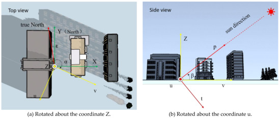
Figure 3.
Illumination point identification and axis transform operations.

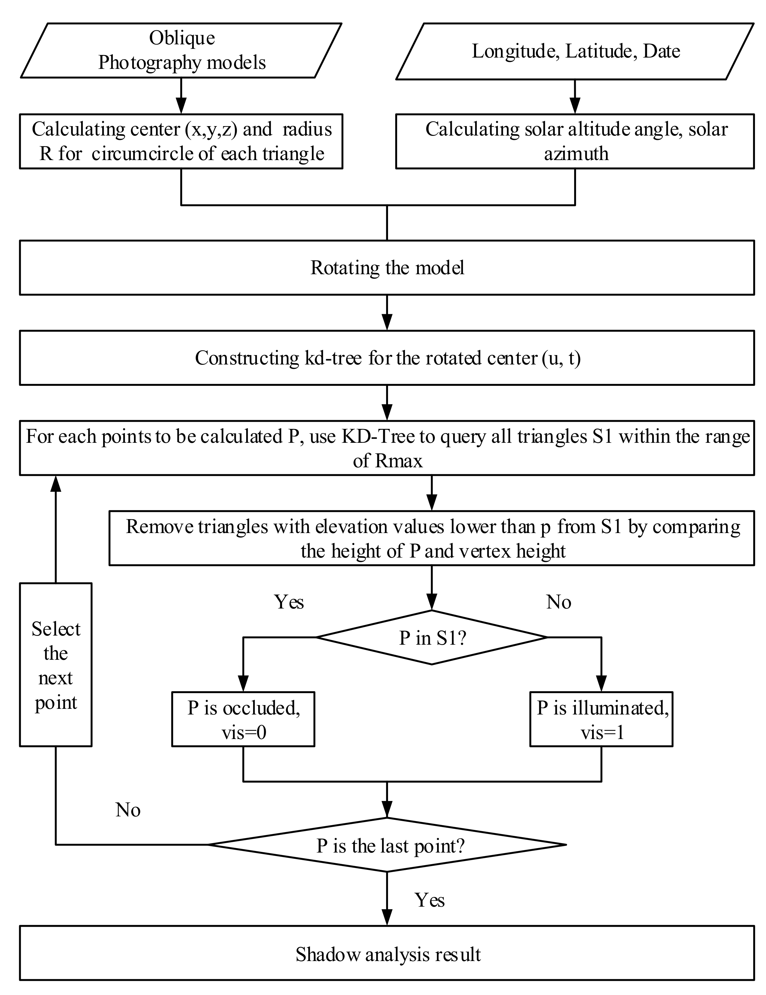
Figure 4.
The flowchart of the hierarchical shading analysis.
The input of the hierarchical shading analysis method consisted of the photogrammetric mesh models, local longitude, and latitude. The date of the shadow simulation needed to be determined. According to the date, the local latitude and longitude, local sun altitude angle, and azimuth angle were then calculated [37]. To speed up the subsequent triangle processing, we pre-calculated the coordinate (u, t) of the circumscribed circle center of each triangle in the photogrammetric mesh models and used it to represent the triangle. The maximum radius of the circumferential circle Rmax was also stored.
An axis transformation was then applied to the input models so that one of the axes of the transformed coordinate system was directed towards the sun. The transformation is described by Equation (6). As shown in Figure 3a,b, the rotation was performed in two stages. The first step was to rotate about the z-axis, changing the coordinate system from o-xyz to o-uvz. The second step was to rotate about the u-axis, changing the coordinate system o-uvz to o-utp. The axis p was therefore parallel to the direction vector of the sun’s rays.
where α is the solar azimuth, β is the solar elevation angle, ε is the angle between the northing direction of the projected coordinate system and the true North direction.
The next step was to create a KD-Tree for the coordinates (u, t) of the triangle circumscribed center. The purpose of establishing a KD-Tree is to facilitate the quick query of the surrounding points. To ensure that the occlusion analysis process does not miss triangles that may cause occlusion, Rmax was used as the search radius. As illustrated in Figure 5a, the adjacent triangle cluster S1 of point P was searched in the two-dimensional space. The triangles below point P were filtered based on the elevation value, as the red triangles in Figure 5b were below the current point P. The remaining triangles, as shown by the blue color in Figure 5b, were those that might occlude point P. It was then determined whether P was in the shadow by determining whether the P point was inside the remained triangles. If any triangle contains P, then P was occluded, and it was illuminated otherwise. The process was ended after processing all the points.
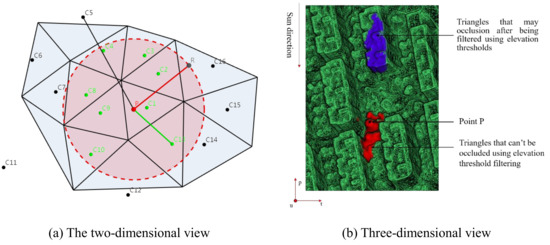
Figure 5.
Illustration of occlusion analysis.
2.2.4. Sky Viewshed Analysis
Buildings also receive scattering irradiance in addition to the total radiation in the atmosphere. The received scattering irradiance of the buildings is related to their visual range in the sky. The sky view of a building and hence its diffused radiation is reduced if it is obstructed by nearby buildings, trees, or other objects. To calculate the solar scattering radiation received by a building, the sky-visible range of that building point needs to be analyzed. The sky view factor (SVF) is commonly used to analyze the obstacles caused by “self-shadows” or adjacent objects. The SVF is time-independent and depends on the environment [40]. Since the changes in the urban scene often happen in longer time scales, it is reasonable to assume a fixed environment while estimating the potential achievable solar energy for the buildings in shorter time scales, for example, on a daily or monthly basis.
The SVF was calculated using Equation (7). Because the sky hemisphere is a continuous space, it is difficult to calculate the scope of the sky horizon. For calculating the sky view for a point in space, the first step was to find all the points within 100 m around that point. The candidate points were then converted into spherical coordinates with the origin set as that point. Then, as also shown in Figure 6, the hemispheres of the sky were horizontally divided into discrete areas at 10° intervals to calculate the maximum occlusion angle in each direction. In choosing a suitable angular interval, we noted that a rather small angular interval affects the calculation efficiency, whereas selecting a too-large angular interval reduces the accuracy of the calculation. To keep the balance between calculation accuracy and efficiency, we chose a 10-degree angle to divide the sky hemisphere. To see other classification methods see, for example, [22].
where represents azimuth, is the zenith angle, and is the maximum occlusion angle in the azimuth direction.
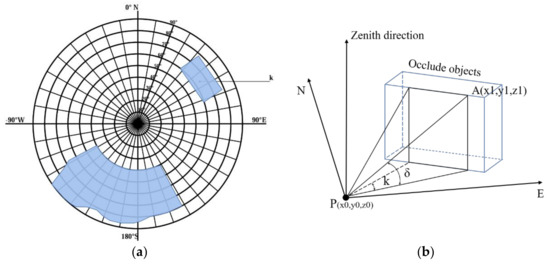
Figure 6.
An illustration of the calculation of the SVF (k: azimuth angle (the angle between k and the north being ); : is the maximum shading angle). (a) Division of the sky hemisphere at equal intervals of 10°. (b) Calculation of the maximum occlusion angle in the k direction.
3. Experimental Results
3.1. Study Area
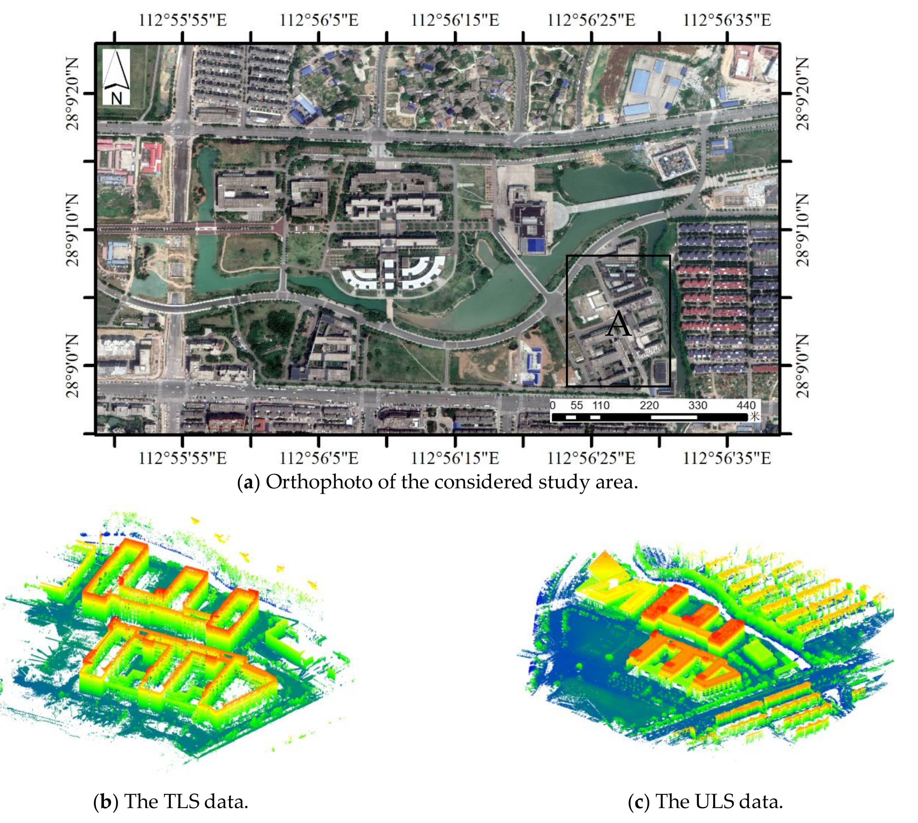
In this paper, we considered the campus of Central South University in Changsha, Hunan Province, China. As seen in Figure 7a, the considered area is approximately 1.2 km2 and consists of various types of buildings. This area mainly includes low raise single buildings with a large area. There is also a densely built residential district in the eastern part of the study area. The tallest building in the study area is 37 m which is located in the southwest corner of the campus. The buildings in this area have large surface areas for the development and utilization of solar energy. Therefore, assessing the potential achievable solar energy of this area can effectively explore the solar energy utilization of buildings.
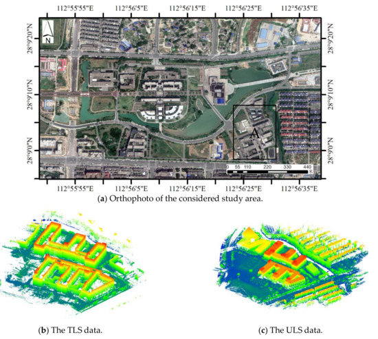
Figure 7.
Experimental data.
As shown in Table 2, the oblique images of this area were obtained on 16 April 2019, and the spatial resolution of the image was 3.5 cm. The resolution of the photogrammetric mesh models established by the oblique image is larger than 10 cm. To verify the effectiveness and reliability of the solar irradiance calculations based on photogrammetric mesh models, we collected the UAV laser scanning (ULS) data and TLS data of area A (see Figure 7b,c). The vertical and horizontal accuracies of the ULS data and TLS data were within 5 cm, and 5 mm, respectively.
Table 2.
System parameters of the oblique photogrammetry system.
3.2. Experimental Results
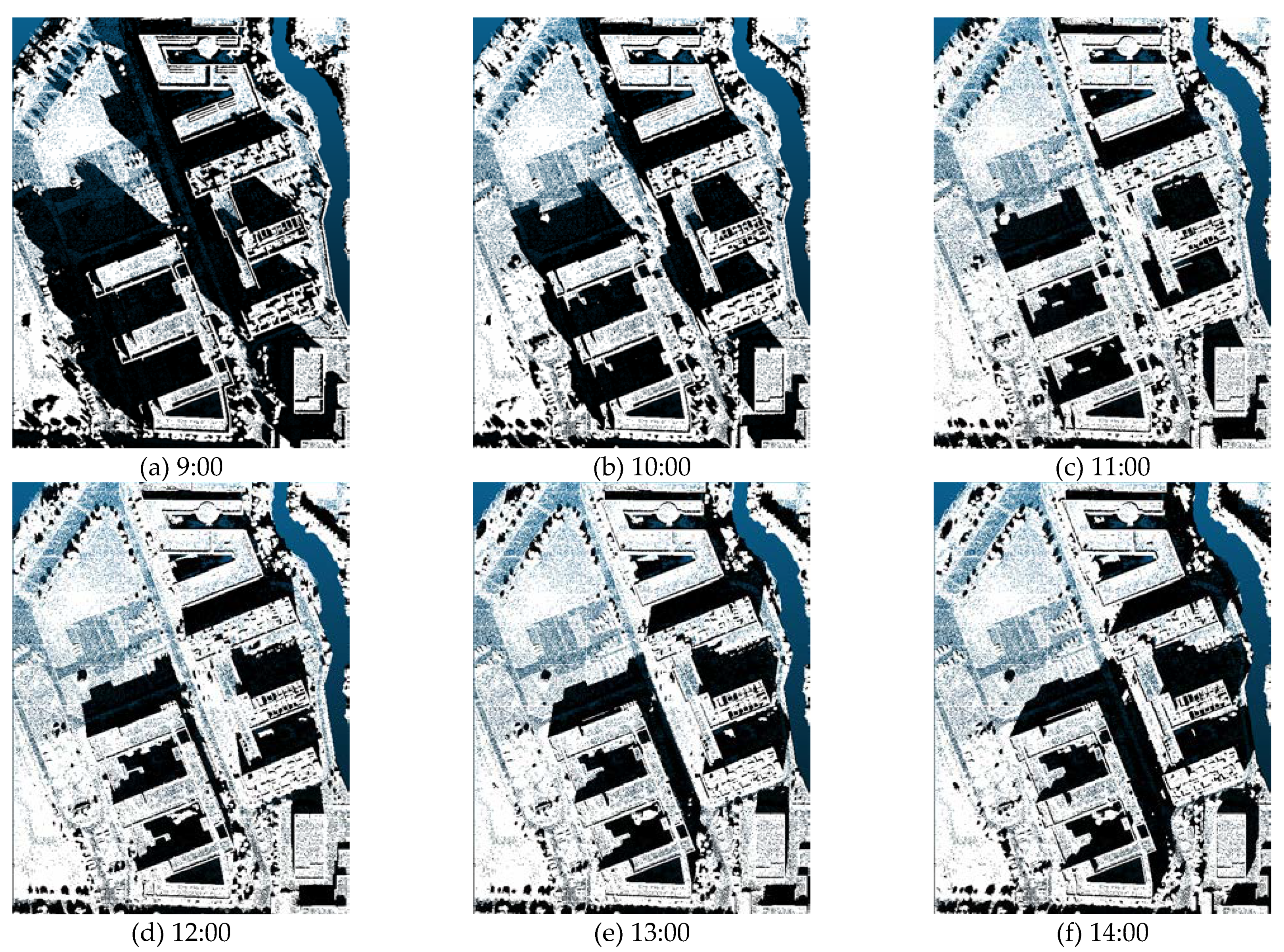
As shown in Figure 8, the shadow area on the surface of the buildings continuously changes throughout the day. The black color indicates that the area is in the shadow, and the white color indicates that the area is illuminated by the sun. Note that the change in the shadow area on the roof is not obvious. This is because most of the time the roof is exposed to direct sunlight. It can also be seen in Figure 8a–d that variations of the shadow area on the building’s facade are more significant, as it is affected by the surrounding trees and the building itself.
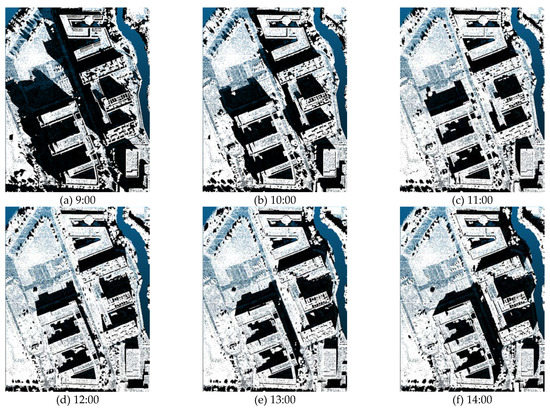
Figure 8.
The shadows of the buildings during the winter solstice in 2019.
The SVF calculation result is shown in Figure 9. In Figure 9, the lighter the color, the larger the visible sky field, while the darker the color, the smaller the visible sky field. An SVF value of 0 indicates that the sky is completely obstructed at that location, whereas an SVF value of 1 indicates that a total view of the sky hemisphere above the horizon is available at that location. Figure 9b shows that the SVF value on the facade is generally lower than that on the roof because at least half of the sky view on the facade is blocked.
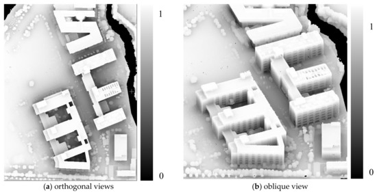
Figure 9.
The calculated results of SVF.
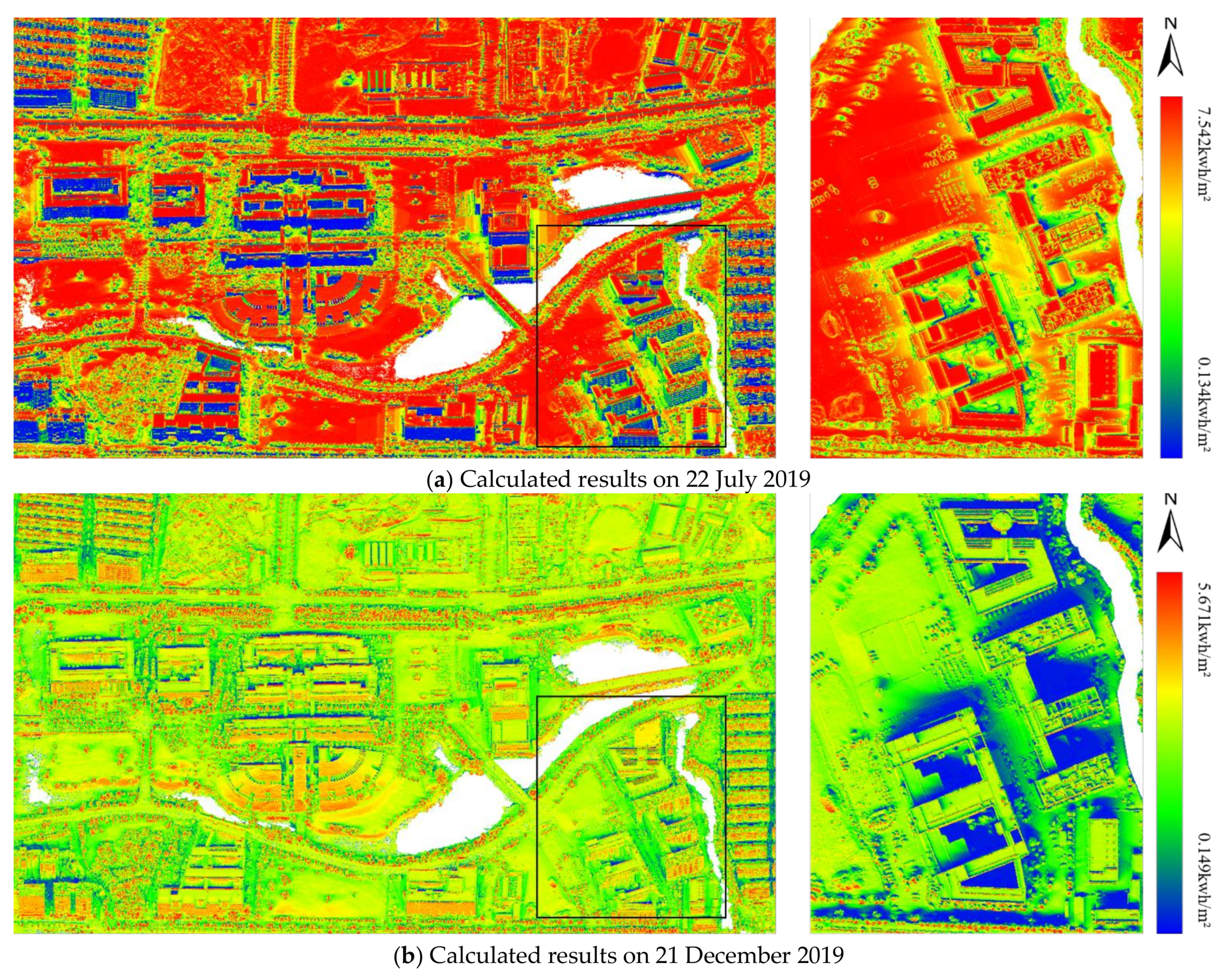
Figure 10 shows the global solar irradiance received at the surface on 21 December and 22 July 2019. The left pictures are oblique views and the right ones are orthogonal views. The solar potential of the building surface is not evenly distributed due to the shadow of the surrounding environment. The color of each point in Figure 8 indicates the received value of solar irradiance throughout the day. Since the calculation results are displayed in a point cloud, they can provide the solar energy in the building for each of the point elements. The maximum cumulative solar irradiance at winter solstice and summer solstice are 5.671 kWh/m2 and 7.542 kWh/m2, respectively. The minimum values are 0.149 kWh/m2 and 0.134 kWh/m2, respectively.

Figure 10.
The cumulative solar irradiance received by the surface of the study area.
3.3. Validation by Comparison Analysis
3.3.1. Comparison with the Shadow in the Photo
The available experimental data do not fully cover the experimental area. Therefore, we focused on area A and used real UAV images to verify the reliability and effectiveness of the proposed method in this paper. The shadow of the object in the image can be regarded as ground truth data of the shadow area. The assessment of our simulated shadow was carried out by comparing the simulated shadow with the corresponding picture taken by the UAV. Figure 11a is the image taken at 11: 25 am on 31 October 2019, in area A, and Figure 11b is the shadow calculated at the time of capturing the image using the proposed method. The agreement between the simulated result and the ground truth image is highlighted at six marked locations. The shaded areas in Figure 11(1)–(6) are caused by the building itself. Beyond the six marked shadow areas, the calculated shadows formed by the trees are also very close to the real shadows.
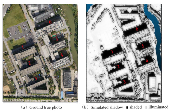
Figure 11.
Shadow simulation against orthoimage (time: 11:25 on 31 October 2019).
3.3.2. Comparing with Other Method Calculation Results
In order to verify the efficiency of the hierarchical shadow analysis method, the shadow simulation calculation time of the hierarchical shadow analysis method in the same region was compared with that of the method proposed by Vo (hereinafter referred to as APM) [31]. The APM method can directly calculate the point cloud data, which is similar to the hierarchical shadow analysis. Both methods were implemented in Python without GPU-accelerated parallel computation. The average computing time of one shadow simulation in the APM method was 35 min, while the hereinafter shadow analysis method was 9 min. The average calculation time difference between the two methods was nearly four times. The two methods were calculated on the same computer, the computer configuration was CPUInter®CoreTM i7-8700, 32GB RAM.
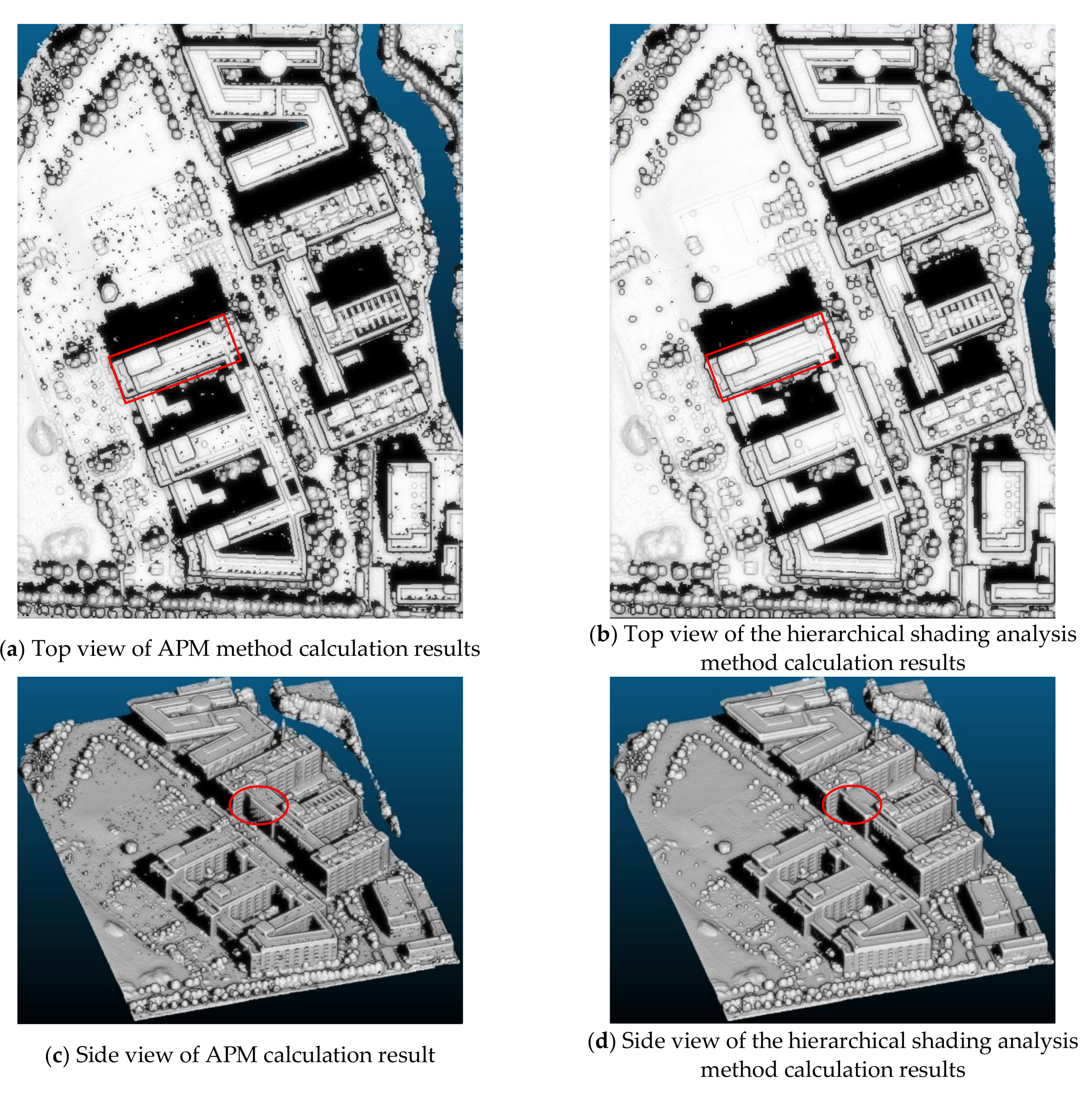
The calculation results of the two methods are shown in Figure 12. It can be seen from the comparison results that the shadow simulation results of the two methods are generally similar, but there are slight differences in particular locations. As shown in Figure 12a, there are some shadow noise points in the calculation results of the APM method on the roof of the building, and the shadow of the building facade simulated by the APM method in Figure 12c appears jagged. The main reason is that the DBSCAN algorithm was used in the APM method for clustering. The clustering parameters of the algorithm are difficult to control, so there is a small number of shadow noise points. However, this situation does not exist in the calculation results of the hierarchical shadow analysis method, and the calculation time of the hierarchical shadow analysis method was much shorter.
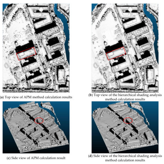
Figure 12.
Comparison of shadow simulation results with other methods.
3.3.3. Comparison with the Solar Irradiance Calculated by ArcGIS
Here, the rooftop solar irradiance results calculated by ArcGIS were used to verify the proposed method. The Solar Analysis Tool (SAT) within the ArcGIS software suite is often used to study the irradiance based on DSM calculations [41]. However, the ArcGIS SAT method cannot analyze the solar radiation on the buildings’ facades, and it is also difficult to perform solar irradiance calculations in ArcGIS SAT on buildings across a large area. Here, we randomly sampled 303 points on the roof of area A and compared them with the results of ArcGIS STA to verify the reliability of the proposed method.
The monthly average of the irradiance calculated in 2019 by the proposed method and ArcGIS SAT are presented in Figure 13, the standard deviation of the estimated solar irradiance is also presented. The monthly average of direct radiation and diffuse radiation irradiance calculated using the proposed method was slightly higher than that of the ArcGIS SAT method, but they showed similar trends. For instance, the maximum solar irradiance received on the rooftops by both methods was in July at 223.10 kWh/m2 and 192.945 kWh/m2, respectively. From January to July, the solar irradiance on the rooftops shows an increasing trend and then declines until December, which is the month with the lowest solar irradiance in the year. The global irradiance calculated by the proposed method and ArcGIS in December was 95.139 kWh/m2 and 56.691 kWh/m2, respectively. The reason for the difference between the obtained results of the two methods is that the selected models are different. As mentioned in the introduction of the solar radiation model, there are several types of solar radiation models, and the results calculated based on different models tend to be different. To see comparisons between different models see Mghouchi’s work in [36].
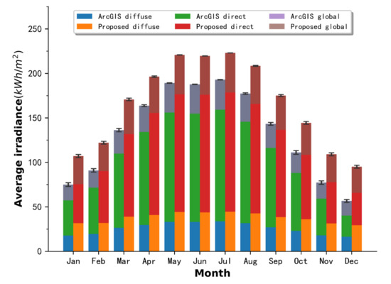
Figure 13.
Comparison of monthly solar irradiance calculated by the proposed method and ArcGIS methods in area A.
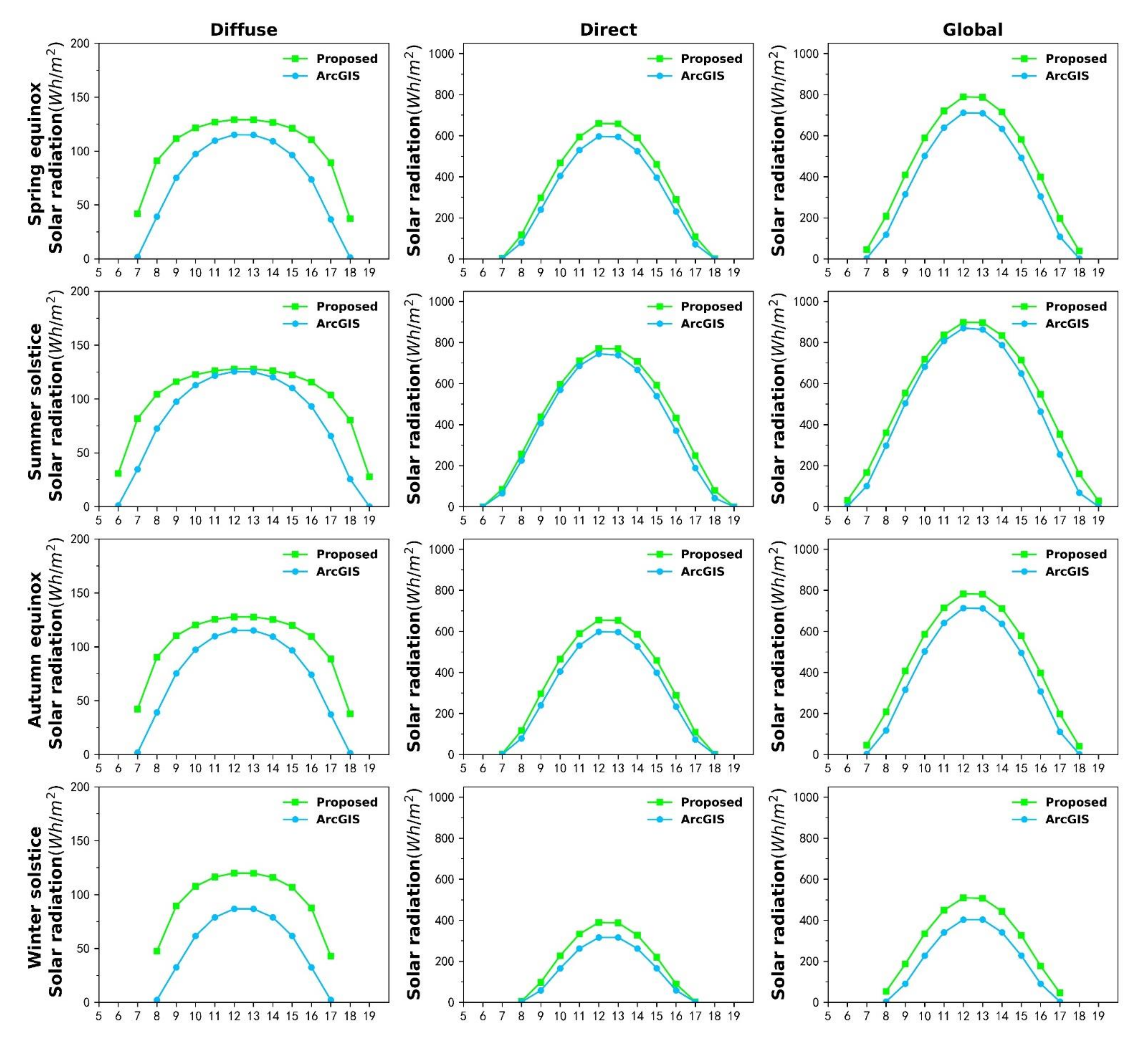
To analyze the difference between the two methods, we also compared the diffuse radiation, direct radiation, and global radiation at different times of the day during the spring equinox, summer solstice, autumn equinox. and winter solstice, as shown in Figure 14. The reason for choosing these four particular days was that the position of the sun is typical during these days. The simulations were performed every hour from sunrise to sunset. We also assumed these four days to have sunny weather.
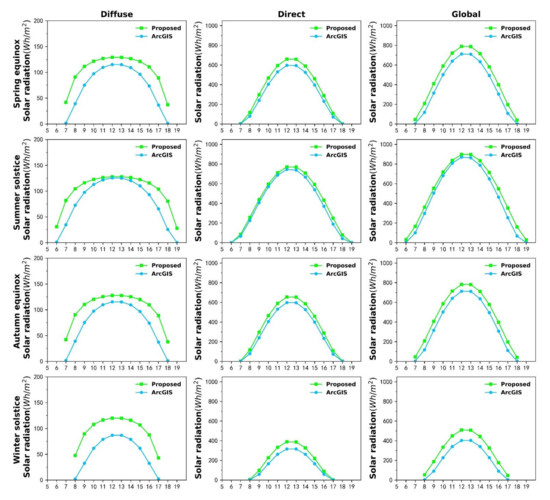
Figure 14.
Comparison of diffuse radiation, direct radiation, and global radiation on four specific days.
It was seen that the direct radiation and diffuse radiation calculated by the proposed method during the summer solstice were the closest to the calculation results of ArcGIS. The difference in the winter solstice was also greater than that of the summer solstice. The difference in the global solar radiation calculated by the two methods on the summer solstice was 0.66 kWh/m2, whereas the difference of diffuse radiation was 0.307 kWh/m2 and the difference of direct radiation was 0.293 kWh/m2. The global irradiance received at the roof on the summer solstice was significantly higher than that of other days, which is indicated as a larger peak in Figure 14. This result corresponds to the previous monthly average solar irradiance result. Furthermore, the solar irradiance received at the roof of the spring equinox and the autumnal equinox was approximately the same. This is explainable because at the spring equinox or at the autumn equinox, the solar altitude angles are approximately equal at the corresponding moments of the day.
Table 3 presents the data for the total diffuse, direct, and global radiation received at the rooftop point within four particular days. The maximum values of direct and diffuse radiation are both occurring at the noon. It is worth noting that although the diffuse radiation value is small, the cumulative difference within a day is not ignorable. In summary, the proposed method and ArcGIS SAT method closely follow the same trends in estimating the solar irradiance on the roofs.
Table 3.
Irradiation result comparison within a day.
3.3.4. Comparison with the Results Using LiDAR Data
As it was mentioned before, LiDAR data can be also used to estimate the achievable potential solar energy of the buildings due to their high accuracy. Here, we adopted the ULS and TLS data as shown in Figure 7 to verify the reliability of the calculation results based on the photogrammetric mesh models. The ULS and TLS data were registered well by manual work and refined using the ICP algorithm. A TIN model was constructed from the fused point cloud using the Poisson surface reconstruction method [42]. The irradiance on the winter solstice for both models was also calculated using the proposed method.
To compare the difference between the two calculation results, we sampled 525 and 592 corresponding location points on the facade and roof of the photogrammetric mesh and the LiDAR models, respectively. The correlation between the two calculation results is shown in Figure 15. As can be seen, the solar irradiance results calculated by the two data sources were highly correlated, and the correlation coefficients (R2) of the calculation results of the facade and roof were 0.9164 and 0.9022.
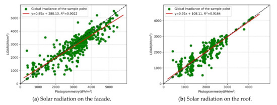
Figure 15.
Correlation analysis.
The comparison result is illustrated in Table 4. Three statistical indicators were adopted to make a quantitative comparison between the results of the photogrammetric mesh models and the LiDAR reference results. The LiDAR and photogrammetric mesh models showed minor differences in both their maximum and minimum values. The Mean Bias Error (MBE) of all points was also obtained using Equation (8).
Table 4.
Comparison of the solar irradiance for LiDAR and photogrammetric mesh models.
Where is the number of point clouds, represents the calculation result of photogrammetric mesh models, represents the calculation result of LiDAR.
The MBE values on the roof and facade were 180.08 and −27.19 Wh/m2, respectively. The comparison results also showed that despite the lower accuracy of oblique photogrammetry compared with LiDAR data, the difference in accuracy had no significant impact on the estimated solar potential of buildings. Overall, the solar irradiance calculated based on the photogrammetric mesh models and the model established from LiDAR data showed similar trends. Therefore, it is reasonable to use photogrammetric mesh models for estimating the achievable potential solar power on the roof and facade.
3.4. Application and Analysis
Having demonstrated the effectiveness and reliability of the proposed method, this section analyzes the changes of irradiance on the roof and facade over various time scales including hourly, daily, monthly and yearly changes on the roof and facade.
The following results were obtained by taking the library of the new campus of Central South University as the research object. Since there is no shelter around this building by other objects, only the effect of its own shadow was taken into consideration. Note that, for buildings with complex surroundings, it is necessary to analyze them in combination with the actual environment.
3.4.1. Hourly Solar Irradiance Analysis
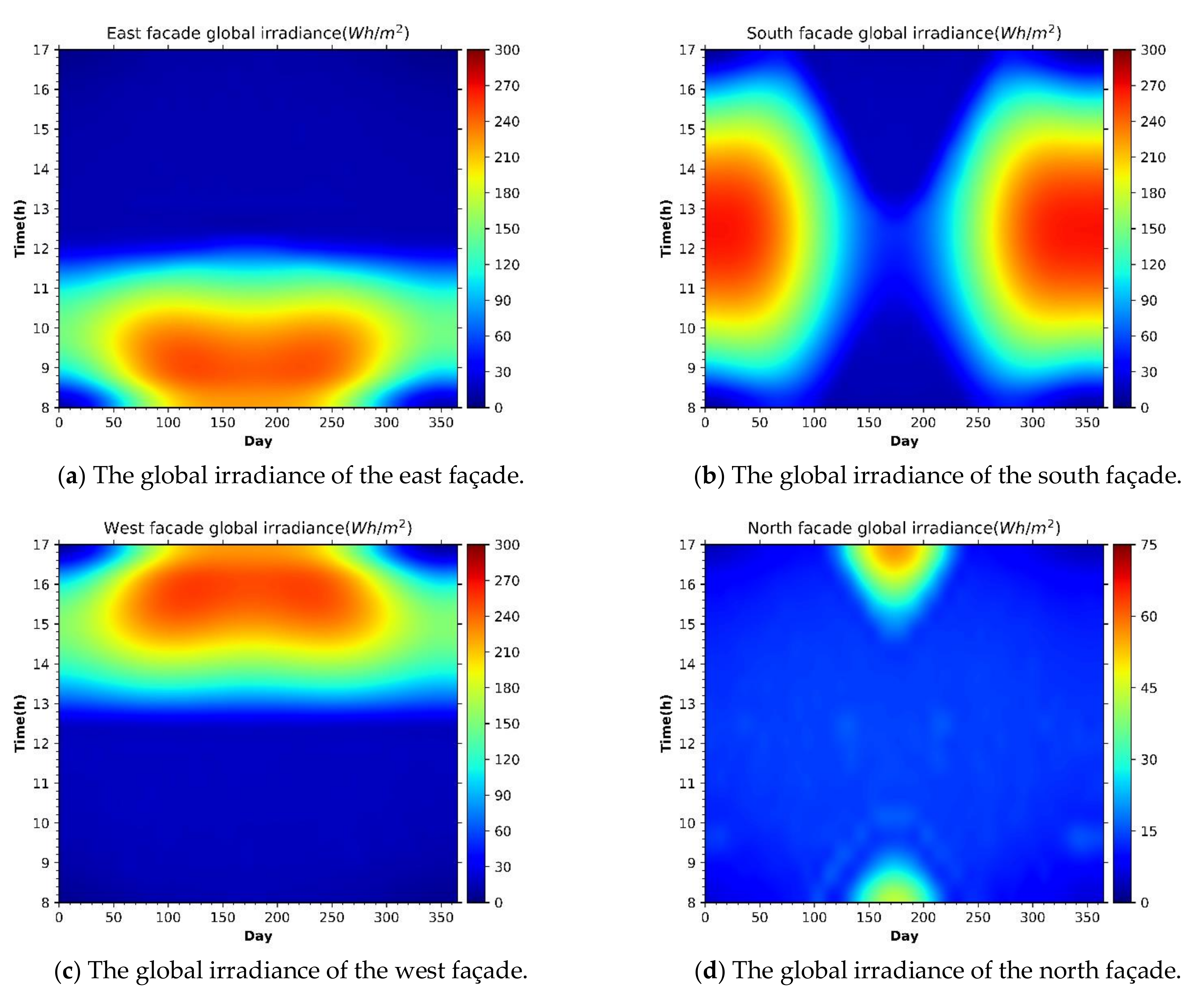
Here, we analyzed the hourly variation of solar irradiance. Affected by solar elevation angle and azimuth, the solar irradiance received on the surface of the buildings is different every day. Therefore, we carried out statistical analysis on hourly variations in the irradiance on the facade. Figure 16 shows the hourly solar irradiance variations in different facade directions from 8:00 am to 5:00 pm every day.
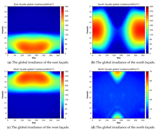
Figure 16.
Global irradiance per hour in different directions.
When the sun rises in the morning, the entire east-facing facade is illuminated. By changing the position of the sun, the east-facing facade gradually loses sunlight (see, Figure 16a). Most of the solar irradiance received from the east-facing facade is concentrated in the period of 8:00–12:00, the rest of the time only diffuse radiation exists. The maximum instantaneous global solar irradiance received on the east-facing facade is 249 wh/m2, which is around 10:00. The west-facing facade is opposite to the east-facing facade, the solar irradiance value received on the west-facing facade is also close to that of the east-facing facade but the time is opposite, as illustrated in Figure 16c. The west-facing facade receives direct sunlight from 13:00 to 17:00, the received irradiance is larger than other periods and the maximum instantaneous global irradiance value is 254 wh/m2. Unlike the east-facing and west-facing facade, the hourly global irradiance on the south-facing facade has greater variations. Except in the summer, when the south-facing facade is illuminated by sunlight during the period from 9:00 am to 4:00 pm. Therefore, the daily sunlight time on the south-facing facade is the largest amongst the four directions (see, Figure 16b). The maximum instantaneous global irradiance value received on the south-facing facade is 268 kW/m2, which is slightly larger than that of the east and west. As the solar elevation angle is larger in summer, the incidence angle of solar rays on the south-facing facade is also larger although the solar irradiance received is smaller. The north-facing facade has the smallest solar irradiance in four directions and as seen in Figure 16d, its illuminated time is also very short.
3.4.2. Daily Solar Irradiance Analysis
Figure 17 shows the variations of total solar irradiance for each day of a year. The plotted curve is the result of interpolation based on the calculated values on certain dates. Comparing the solar irradiance results on the roof (Figure 17a) and the facade (Figure 17b) it is seen that only the south-facing facade receives solar irradiance greater than the roof on a few days in a year. The other directions facades receive much less solar irradiance than the roof.
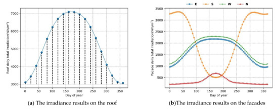
Figure 17.
Polynomial interpolation of the daily total irradiation.
3.4.3. Monthly and Annual Average Solar Irradiance
The monthly global irradiance variations on roofs and facades are also shown in Figure 18. The global irradiance on the roof reached its maximum in July (223 kWh/m2) and minimum in December (95 kWh/m2). From January to July, the monthly global solar irradiance on the roof increased on monthly basis and gradually decreased from July to December. The global irradiance received on the library roof within a year was 1995 kWh/m2, of which direct irradiance was 1541 kWh/m2 and diffuse radiation was 454 kWh/m2, accounting for 77% and 23% of the global irradiance, respectively.
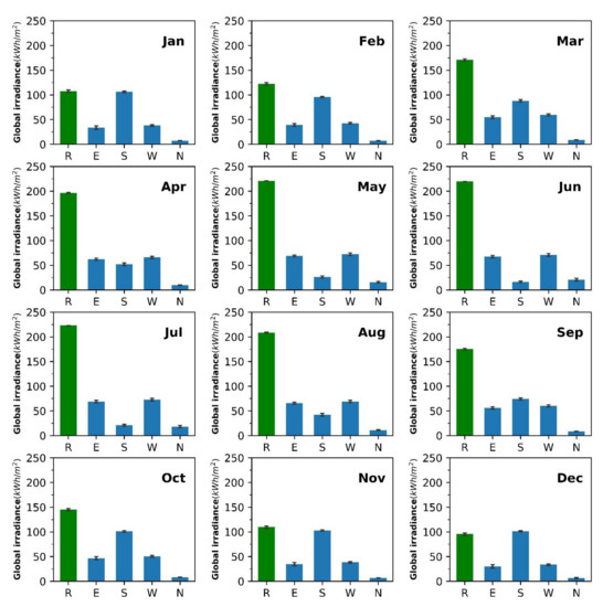
Figure 18.
Variation of the monthly solar radiation on the roof and four facades.
The east-facing and west-facing facades were also consistent with the roof, which reached its maximum and minimum global irradiance in July and December, respectively. The difference is that the global irradiance received on the east-facing and west-facing facades was much smaller than that of the roof. The global irradiance received on the facade of east-facing and west-facing in a year was 628 kWh/m2 and 674 kWh/m2, respectively. The global irradiance of the north-facing facade was small for each month, and the global irradiance in a year was only 127 kWh/m2, which is less than 1/10 of that of the roof. The south-facing facade reached global irradiance maximum in January (106 kWh/m2) and minimum in June (16 kWh/m2). The global irradiance received on the south-facing facade in a year was 827 kWh/m2, which is the largest amongst the four directions.
4. Conclusions
In this paper, we proposed a method for the efficient assessment of solar irradiance on a building in urban areas. The proposed method estimates the potential achievable solar energy of the buildings based on photogrammetric mesh models, which provides new data for estimating the solar energy potential of buildings. To improve the efficiency of shadow simulation with photogrammetric mesh models, we also proposed a hierarchical shadow analysis method to address the issue of low efficiency of shadow analysis caused by a large number of triangular nets in photogrammetric mesh models. The proposed method minimizes the judgment of redundant triangles and improves the calculation speed by rotating the model and setting the height threshold. The shadow simulation results were also verified on the real image. The solar irradiance calculated by the photogrammetric mesh models was also compared with that calculated by LiDAR data, and it was shown that the two calculated results are very similar. In conclusion, photogrammetric mesh models can be used to comprehensively estimate the solar energy potential of the building.
Author Contributions
Conceptualization, Y.Z., W.W., X.L., and L.C.; methodology, Z.D. and L.C.; software, Z.D.; validation, Z.D. and L.C.; resources, W.W. and X. L.; writing—original draft preparation, Y.Z., Z.D., and L.C.; writing—review and editing, Y.Z., S.C., and L.C.; All authors have read and agreed to the published version of the manuscript.
Funding
This research was funded by the University Innovative Platform Open Fund of Hunan (No. 19K099), the Natural Science Foundation of China (No. 41971341 and 41971354), Open Fund of Key Laboratory of Urban Land Resource Monitoring and Simulation, Ministry of Land and Resource (No. KF-2018-03-047).
Acknowledgments
We thank Qing Zhu for his very useful comments and suggestions on the paper.
Conflicts of Interest
The authors declare no conflict of interest.
References
- Cheng, L.; Zhang, F.; Li, S.; Mao, J.; Xu, H.; Ju, W.; Liu, X.; Wu, J.; Min, K.; Zhang, X.; et al. Solar energy potential of urban buildings in 10 cities of China. Energy 2020, 196, 117038. [Google Scholar] [CrossRef]
- Lingfors, D.; Bright, J.; Engerer, N.; Ahlberg, J.; Killinger, S.; Widén, J. Comparing the capability of low-and high-resolution LiDAR data with application to solar resource assessment, roof type classification and shading analysis. Appl. Energy 2017, 205, 1216–1230. [Google Scholar] [CrossRef]
- Voegtle, T.; Steinle, E.; Tóvári, D. Airborne laserscanning data for determination of suitable areas for photovoltaics. ISPRS-J. Photogramm. Remote Sens. 2012, 36, 215–220. [Google Scholar]
- Yu, B.; Liu, H.; Wu, J.; Lin, W.-M. Investigating impacts of urban morphology on spatio-temporal variations of solar radiation with airborne LiDAR data and a solar flux model: A case study of downtown Houston. Int. J. Remote Sens. 2009, 30, 4359–4385. [Google Scholar] [CrossRef]
- Hofierka, J.; Kaňuk, J. Assessment of photovoltaic potential in urban areas using open-source solar radiation tools. Renew. Energy 2009, 34, 2206–2214. [Google Scholar] [CrossRef]
- Redweik, P.; Catita, C.; Brito, M. Solar energy potential on roofs and facades in an urban landscape. Sol. Energy 2013, 97, 332–341. [Google Scholar] [CrossRef]
- Jakubiec, J.; Reinhart, C. A method for predicting city-wide electric production from photovoltaic panels based on LiDAR and GIS data combined with hourly DAYSIM simulations. Sol. Energy 2013, 93, 127–143. [Google Scholar] [CrossRef]
- Bayrakci, M.; Calvert, K.; Brownson, J. An automated model for rooftop PV systems assessment in ArcGIS using LiDAR. AIMS Energy 2015, 3, 401–420. [Google Scholar] [CrossRef]
- Lukac, N.; Seme, S.; Dežan, K.; Zalik, B.; Stumberger, G. Economic and environmental assessment of rooftops regarding suitability for photovoltaic systems installation based on remote sensing data. Energy 2016, 107, 854–865. [Google Scholar] [CrossRef]
- Huang, Y.; Chen, Z.; Wu, B.; Chen, L.; Mao, W.; Zhao, F.; Wu, J.; Wu, J.; Yu, B. Estimating roof solar energy potential in the downtown area using a GPU-accelerated solar radiation model and airborne LiDAR data. Remote Sens. 2015, 7, 17212–17233. [Google Scholar] [CrossRef] [Green Version]
- Mansouri Kouhestani, F.; Byrne, J.; Johnson, D.; Spencer, L.; Hazendonk, P.; Brown, M. Evaluating solar energy technical and economic potential on rooftops in an urban setting: The city of Lethbridge, Canada. IJEEE 2018, 10, 13–32. [Google Scholar] [CrossRef] [Green Version]
- Lee, J.; Zlatanova, S. Solar radiation over the urban texture: LiDAR data and image processing techniques for environmental analysis at city scale. In 3D Geo-Information Sciences. Lecture Notes in Geoinformation and Cartography; Springer: Heidelberg/Berlin, Germany, 2009; pp. 319–340. [Google Scholar]
- Catita, C.; Redweik, P.; Pereira, J.; Brito, M.C. Extending solar potential analysis in buildings to vertical facades. Comput. Geosci. 2014, 66, 1–12. [Google Scholar] [CrossRef]
- Desthieux, G.; Carneiro, C.; Camponovo, R.; Ineichen, P.; Morello, E.; Boulmier, A.; Abdennadher, N.; Dervey, S.; Ellert, C. Solar energy potential assessment on rooftops and facades in large built environments based on LiDAR data, image processing, and cloud computing. Methodological background, application, and validation in geneva (Solar cadaster). Front. Environ. Sci. 2018, 4, 14. [Google Scholar] [CrossRef]
- Li, Z.; Zhang, Z.; Davey, K. Estimating geographical PV potential using LiDAR data for buildings in downtown San Francisco. Trans. GIS 2015, 19, 930–963. [Google Scholar] [CrossRef]
- Zhang, X.; Lv, Y.; Tian, J.; Pan, Y. An Integrative approach for solar energy potential estimation through 3D modeling of buildings and trees. Can. J. Remote Sens. 2015, 41, 126–134. [Google Scholar] [CrossRef]
- Jochem, A.; Höfle, B.; Rutzinger, M. Extraction of vertical walls from mobile laser scanning data for solar potential assessment. Remote Sens. 2011, 3, 650–667. [Google Scholar] [CrossRef] [Green Version]
- Huang, P.; Cheng, M.; Chen, Y.; Zai, D.; Wang, C.; Li, J. Solar potential analysis method using terrestrial laser scanning point clouds. IEEE J. Sel. Top. Appl. Earth Observ. 2017, 10, 1221–1233. [Google Scholar] [CrossRef]
- Liang, F.; Yang, B. Multilevel solar potential analysis of building based on ubiquitous point clouds. In Proceedings of the 2018 26th International Conference on Geoinformatics, Kunming, China, 28–30 June 2018; pp. 1–4. [Google Scholar]
- Qin, R.; Gruen, A. 3D change detection at street level using mobile laser scanning point clouds and terrestrial images. ISPRS-J. Photogramm. Remote Sens. 2014, 90, 23–35. [Google Scholar] [CrossRef]
- Xiao, W.; Vallet, B.; Schindler, K.; Paparoditis, N. Street-side vehicle detection, classification and change detection using mobile laser scanning data. ISPRS-J. Photogramm. Remote Sens. 2016, 114, 166–178. [Google Scholar] [CrossRef]
- Freitas, S.; Catita, C.; Redweik, P.; Brito, M.C. Modelling solar potential in the urban environment: State-of-the-art review. Renew. Sust. Energy Rev. 2015, 41, 915–931. [Google Scholar] [CrossRef]
- Zhao, P. A UAV-based panoramic oblique photogrammetry (POP) approach using spherical projection. ISPRS-J. Photogramm. Remote Sens. 2019, 159, 198–219. [Google Scholar]
- Zhu, Q.; Wang, Z.; Hu, H.; Linfu, X.; Ge, X.; Zhang, Y. Leveraging photogrammetric mesh models for aerial-ground feature point matching toward integrated 3D reconstruction. ISPRS-J. Photogramm. Remote Sens. 2020, 166, 26–40. [Google Scholar] [CrossRef]
- Zhu, Q.; Shang, Q.; Hu, H.; Yu, H.; Zhong, R. Structure-aware completion of photogrammetric meshes in urban road environment. ISPRS-J. Photogramm. Remote Sens. 2021, 175, 56–70. [Google Scholar] [CrossRef]
- Ostrowski, W. Accuracy of measurements in oblique aerial images for urban environment. ISPRS—Int. Archives Photogrammetry Remote Sens. Spat. Inf. Sci. 2016, XLII-2/W2, 79–85. [Google Scholar] [CrossRef] [Green Version]
- Yalcin, G.; Selcuk, O. 3D city modelling with oblique photogrammetry method. Phys. Procedia 2015, 19, 424–431. [Google Scholar] [CrossRef] [Green Version]
- Menouar, H.; Guvenc, I.; Akkaya, K.; Uluagac, S.; Kadri, A.; Tuncer, A. UAV-enabled intelligent transportation systems for the smart city: Applications and challenges. IEEE Commun. Mag. 2017, 55, 22–28. [Google Scholar] [CrossRef]
- Ratti, C.; Sabatino, S.D.; Britter, R. Urban texture analysis with image processing techniques: Winds and dispersion. Theor. Appl. Climatol. 2006, 84, 77–90. [Google Scholar] [CrossRef]
- Jochem, A.; Höfle, B.; Rutzinger, M.; Pfeifer, N. Automatic roof plane detection and analysis in airborne Lidar point clouds for solar potential assessment. Sensors 2009, 9, 5241–5262. [Google Scholar] [CrossRef] [PubMed]
- Vo, A.V.; Laefer, D.F.; Smolic, A.; Zolanvari, S.J.I.J.o.P.; Sensing, R. Per-point processing for detailed urban solar estimation with aerial laser scanning and distributed computing. ISPRS-J. Photogramm. Remote Sens. 2019, 155, 119–135. [Google Scholar] [CrossRef]
- Boulch, A.; Marlet, R. Fast and robust normal estimation for point clouds with sharp features. Comput. Graph. Forum 2012, 31, 1765–1774. [Google Scholar] [CrossRef] [Green Version]
- Brito, M.C.; Freitas, S.; Guimarães, S.; Catita, C.; Redweik, P. The importance of facades for the solar PV potential of a Mediterranean city using LiDAR data. Renew. Energy 2017, 111, 85–94. [Google Scholar] [CrossRef]
- Gueymard, C.A. Clear-sky irradiance predictions for solar resource mapping and large-scale applications: Improved validation methodology and detailed performance analysis of 18 broadband radiative models. Sol. Energy 2012, 86, 2145–2169. [Google Scholar] [CrossRef]
- Yao, W.; Li, Z.; Zhao, Q.; Lu, Y.; Lu, R. A new anisotropic diffuse radiation model. Energy Convers. Manag. 2015, 95, 304–313. [Google Scholar] [CrossRef]
- El Mghouchi, Y.; El Bouardi, A.; Choulli, Z.; Ajzoul, T. Models for obtaining the daily direct, diffuse and global solar radiations. Renew. Sust. Energy Rev. 2015, 56, 87–99. [Google Scholar] [CrossRef]
- Kumar, L.; Skidmore, A.; Knowles, E. Modelling topographic variation in solar radiation in a GIS environment. Int. J. Geogr. Inf. Sci. 1997, 11, 475–497. [Google Scholar] [CrossRef]
- Noorian, A.M.; Moradi, I.; Kamali, G.A. Evaluation of 12 models to estimate hourly diffuse irradiation on inclined surfaces. Renew. Energy 2008, 33, 1406–1412. [Google Scholar] [CrossRef]
- Liu, B.; Jordan, R. Daily insolation on surfaces tilted towards equator. ASHRAE J. 1961, 3, 526–541. [Google Scholar]
- Littlefair, P. Passive solar urban design: Ensuring the penetration of solar energy into the city. Renew. Sust. Energy Rev. 1998, 2, 1998. [Google Scholar] [CrossRef]
- ESRI. ArcGIS Desktop: Release 10; Environmental Systems Research Institute: Redlands, CA, USA, 2014. [Google Scholar]
- Kazhdan, M.; Bolitho, M.; Hoppe, H. Screened poisson surface reconstruction. ACM Trans. Graph. 2013, 32, 29. [Google Scholar] [CrossRef] [Green Version]


Publisher’s Note: MDPI stays neutral with regard to jurisdictional claims in published maps and institutional affiliations. |
© 2021 by the authors. Licensee MDPI, Basel, Switzerland. This article is an open access article distributed under the terms and conditions of the Creative Commons Attribution (CC BY) license (https://creativecommons.org/licenses/by/4.0/).