Characterization of Urban Heat Islands Using City Lights: Insights from MODIS and VIIRS DNB Observations

Abstract

An urban heat island (UHI) is a phenomenon whereby the temperature in an urban area is significantly warmer than it a rural area. To further advance the characterization and understanding of UHIs within urban areas, nighttime light measured by the Day/Night Band (DNB) onboard the Visible Infrared Imaging Radiometer Suite (VIIRS) and the land surface temperature (LST) data derived from the Moderate Resolution Imaging Spectroradiometer (MODIS) combined with principal component analysis (PCA) are used here. Beijing (highly developed) and Pyongyang (less developed) are selected as the two case studies. Linear correlation analysis is first used, with higher correlations being found between DNB and LST data at nighttime than between population and LST data for both cities, although none of the correlation coefficients are particularly high because of noise. Principal component analysis (PCA), a method that can remove random noise, is used to extract more useful information. Two types of PCA are conducted, focusing on spatial (S) and temporal (T) patterns. The results of the S-mode PCA reveal that the typical temporal variation is a seasonal cycle for both LST and DNB data in Beijing and Pyongyang. Furthermore, there are monthly cycles for DNB data related to the moon phase in two cities. The T-mode PCA results show important spatial information, while the spatial pattern of the first mode explains over 50% of the variation. This study is among the first to demonstrate the advantages of using urban light to study the spatial variation of urban heat, especially for nighttime urban temperatures measured from space, at the street and neighborhood scales.

1. Introduction

An urban heat island, or UHI, refers to a phenomenon whereby urban areas tend to have higher air or surface temperatures than their surroundings, which is among the most notable aspect of human impacts on the Earth [1,2,3,4,5]. The UHI effect not only alters ecoenvironments, affecting net primary production, biodiversity, water and air quality, and climate [6,7,8,9], but also affects human health and well-being, contributing to increases in morbidity, mortality, and risk of violence [10,11,12]. These impacts are expected to be more severe when compounded by global climate changes [13]; thus, better characterization and understanding of the UHI effects are critically important to support future climate mitigation actions and human adaptive strategies [3,4,14].

The mechanism underlying UHI formation is thought to be an alteration of a biophysical process in nature by frequent human activities. The surface properties in rural and urban areas are significantly different in their sensible heat dissipation, convection efficiency, evaporative cooling, and sunlight reflection. In the daytime, reductions of the sensible heat convection efficiency and evaporative cooling are important contributors to the UHI effect, while at nighttime a major contributor to UHIs is the heat released from energy use and from solar energy stored in buildings [15].

UHIs can be calculated by using either 2 m air temperatures or land surface temperatures (LSTs). Because the data from the former approach suffer from the sparse distribution of in situ weather stations, it cannot provide a full description of the spatial distribution of UHIs. Remote sensing data hold promise for their ability to add information for spatial coverage. To date, the vast majority of climatologic studies of UHIs have been performed using satellite-derived LST data to study surface urban heat islands, as more satellite products are available from space-borne sensors such as the NOAA Advanced Very High-Resolution Radiometer (AVHRR) [16], Moderate Resolution Imaging Spectroradiometer (MODIS) LST [14,17], Landsat TM/ETM+ images [2], the Defense Meteorological Satellite Program (DMSP) [18], and Visible Infrared Imaging Radiometer Suite (VIIRS) [19]. For example, Gallo found that the satellite-derived normalized difference vegetation index (NDVI) is a good indicator of the differences in surface properties between the two environments that are responsible for differences in urban and rural minimum temperatures, using data from AVHRR for 37 cities in the USA [16]. Cao analyzed the annual mean ∆T values measured by the MODIS instrument onboard the Aqua satellite from 2003 to 2013 for 39 cities across mainland China and found that the MODIS-derived nighttime ∆T (3.4 ± 0.2 K, mean ± 1 s.e.) was higher than the daytime value (2.1 ± 0.3 K; p < 0.001) [20].

While the use of satellite data has been a mainstay in UHI characterization, different methods exist. For example, a paper studying UHIs in 39 cities in mainland China selected 3 × 3 pixels from the urban core to represent the whole urban area, while surrounding rural areas were represented by up to four sets of 3 × 3 pixels at the four sides of the city [20]. Another study mapped UHIs from 32 cities in China using cloud-free Landsat TM/ETM+ images at a high spatial resolution of 30 × 30 m and classified land covers into three types (i.e., built-up land, water bodies, and other lands) using the maximum likelihood classification approach [2]. Another study also classified the urban areas using the city clustering algorithm for 419 global cities according to the MODIS land cover map and defined the suburban area as the nonurban pixels (excluding water pixels) within the ring zone around the urban area [1].

Several parameters have been found to have a close correlation with the magnitude of a UHI, such as population. The use of an urban population as a predictor of a UHI has been studied for a long time [4,21,22]; these studies using satellite data found that the magnitude of a UHI on average has a positive correlation with a city population. Hung [23] found that the magnitudes and spatial extents of UHIs in eight selected Asian megacities in both temperate and tropical climate regions had positive correlations as high as 0.47 with respect to the population sizes of the cities during the daytime. For 65 selected cities in North America, the annual mean midnight temperature from the UHI was also positively correlated with the logarithm of the population, with a coefficient of 0.54 [24]; however, limitations to the use of population statistics as estimators of UHIs include the lack of globally consistent statistics. Additionally, the population data given for a geographically arbitrary boundary can be difficult to relate to the population in the immediate vicinity of the weather stations or urban areas. Furthermore, there are no reliable or timely gridded population data available, especially over regions that have experienced rapid urban development, such as in China.

The aim of the present study is to investigate spatial characteristics of the nighttime UHI in a city via combined use of the MODIS LST and VIIRS DNB products, since the latter have been shown to be good surrogates for estimating population and economic activity at national and sub-national scales [25]. Indeed, city light data measured using DMSP have been used to map urban areas from as early as 1997 [26], although the potential to quantitively characterize the variability of the city light intensity is limited due to the lack of calibration and low saturation limit, especially over urban cores [18]. In contrast, the VIIRS onboard the recently launched Suomi-NPP has significant improvements over DMSP in terms of the spatial resolution, radiometric resolution, and calibration, in turn offering an unprecedented opportunity to map the distribution of a population [19].

This study differs from past studies in that it not only characterizes UHIs in terms of the inner-urban scale but also analyzes the extent to which city light data at night can explain the spatial and temporal variability of LST within UHIs, especially at night. By focusing on the application of both DNB and LST data measured nearly simultaneously at night, this study contrasts with the past studies on UHIs, which studied variations of urban-area-averaged UHI effects among different cities with respect to (a) the population or (b) NDVI. Both approaches have disadvantages for studying nighttime UHIs because population data are often static (e.g., not updated in a timely manner by month or by year), while the NDVI is measured during the daytime only and is not concurrent with nighttime satellite measurements. These disadvantages may lead to uncertainties in areas such as Beijing that have had steady and rapid urban growth in the past decades. Beijing, the capital of China, has been expanding over the past three decades by replacing villages and farmlands with high-rise buildings. It has a population of about 21.7 million and is one of the most urbanized and brightest cities in China on clear nights [27]. In addition, to provide contrast analysis for Beijing, Pyongyang is also selected here, the capital of North Korea, with a population of 2.5 million. It is a city that is darker at night and less developed than Beijing, and thereby will enable the analysis of the hypothesis that the distribution and intensity of city lights can be a better surrogate for describing the UHI effect at night. To quantitatively establish the relationships of the spatial and temporal variability between LST and DNB, the principal component analysis (PCA) technique is employed, which has not been used in UHI studies. The rest of this paper is organized as follows. Section 2 introduces the multiple datasets and methods used herein. Section 3 presents the results of the PCA analysis for all datasets and anomalies. The discussion and conclusions are provided in Section 4, respectively.

2. Materials and Methods

2.1. Datasets and Processing

Land surface temperature (LST) data were obtained from the Aqua MODIS 8-day composite products (version 6), with a spatial resolution of 1 × 1 km (MYD11A2). The Aqua MODIS LST data were retrieved from clear-sky (99% confidence) observations monitored at 01:30 and 13:30 local solar time, using a generalized split-window algorithm for the thermal infrared band [28]. The retrieval of LST data was further improved by correcting noise due to cloud contamination, topographic differences, and zenith angle changes. Wan [29] reported that the accuracy of MODIS LST data is better than 1 K for most tested cases, while Rigo [30] found less than a 5% difference between MODIS LSTs and in situ measurements in urban areas. In addition, the reason why the Aqua LST images were chosen instead of the scenes from the Terra platform for this study is that the overpass time for Aqua is much closer to the actual occurrence of observed maximum and minimum temperatures and is also closer (within one hour) to the VIIRS overpass time at night.

The nighttime light intensity data used here were from the Visible Infrared Imager Radiometer Suite (VIIRS) aboard NPP, which was launched on 28 October 2011 and collects high-quality nighttime images at a spatial resolution of 750 m from the day–night band (DNB). The DNB has a unique ability to sense extremely low levels of visible and near-infrared light at nighttime at levels more than 10 million times fainter than reflected sunlight [31]. The DNB also has a measured spectral response of 400–900 nm (full width at half maximum, with a nominal band center wavelength of 705 nm) and features several advances to the heritage DMSP, including full calibration and improved spatial (0.74 km vs. ~3 km) and radiometric (14 bit vs. 6 bit) resolutions [32]. The VIIRS data were released by NOAA/NGDC in early 2013, while the daily cloud-free products used in the current study were obtained from https://www.bou.class.noaa.gov/saa/products/welcome, accessed on 5 July 2021.

The population density data used in the current paper were extracted from the Gridded Population of the World Version 4 (GPWv4) dataset provided by the Center for International Earth Science Information Network of Columbia University (http://sedac.ciesin.columbia.edu/data/collection/gpw-v4, accessed on 5 July 2021) [33]. This dataset is based on Population and Housing Censuses, while the product used here is Population Density v4.10 2015, with a spatial resolution of 30 arc-seconds (approximately 1 km at the equator) [33]. The fourth version of GPW (GPWv4) is a raster data collection of globally integrated national population data from the 2010 round of Population and Housing Censuses, which occurred between 2005 and 2014. The input data are extrapolated as a function of time to produce population estimates for the years 2000, 2005, 2010, 2015, and 2020, which may have large uncertainty in reflecting urban growth. In the current work, gridded population data from 2015 were selected.

MODIS LST and VIIRS data from 2014 to 2016 were re-gridded to a resolution of 2 km, while population data represent the statistical average for 2015 resampled to 2 km. Because LST data are 8-day composite products, VIIRS data here were also processed for 8-day intervals.

2.2. Analysis Method

Linear regression was used firstly to reveal the relationships between LST, DNB, and population data. Since LST, DNB, and population data are all gridded data, the correlation coefficients of LSTs between DNB and population data on all grids were first calculated. The calculations were verified by comparing the results between those using the internal functions in Python and those using the Pearson correlation coefficient. In addition, an advanced statistical technique, principal component analysis (PCA), was used to find the major spatial and temporal variation patterns for nighttime LST and DNB. PCA was invented in 1901 by Karl Pearson [34]. It is a statistical procedure that uses an orthogonal transformation to convert a set of observations of possibly correlated variables into a set of values of linearly uncorrelated variables called principal components. PCA has been traditionally applied to climate variables such as temperature to examine climate modes by filtering the noise into a series of high-order modes while separating signals in the dominant modes [35]; however, researchers have found that it is also suitable for other variables related to air pollution. For example, Li et al. analyzed the spatial and temporal patterns of aerosol optical depth in land and ocean areas with data taken from several different platforms [36].

In addition, the vast majority of applications in meteorology are space–time studies. In such studies, a decision must be made on whether the data will be expressed in an S- or T-mode approach [37], where S and T stand for space and time, respectively. The S-mode treats the time series (m times) of a geophysical parameter at each of the n stations (or grid points) as a data vector in the analysis; n vectors of these variables are then arranged as one data matrix because the domain of interest is the geographical area or space. Conversely, the T-mode treats the spatial field, defined by all n stations (or grid points) for a given time, as one data vector; therefore, data vectors for each of the m time observations can form a data matrix, while the domain of interest is time. If each column of the input data matrix X is treated as one data vector for the variable of interest, X has dimensions of M (rows) × N (columns) for the S-mode representation (hereafter X_S) and N × M for the T-mode (X_T). As a consequence of these definitions, S-mode analysis results in an N × N similarity matrix, as the analysis investigates how temporal changes vary with space (e.g., how the dominant temporal mode is distributed as a function in space), whereas the T-mode results in an M × M similarity matrix, as the analysis investigates how spatial changes vary with time (e.g., how the dominant spatial mode is distributed as a function of time) [38]. The next decision is to select an appropriate similarity matrix. The most common approaches use the covariance or correlation dispersion matrix.

Taking the S-mode of LST data in Beijing as an example, LST data fields can be represented by X with a size of M × N, while each pixel in an observation is a variable, so M (number of times) is the number of observations and N (number of features) is the number of pixels. Then, the PCA is calculated by determining the eigenvectors of the covariance matrix C, which are:

$$\mathrm{C}=\frac{1}{M-1}{X}^{T}X$$

(1)

Here, C is a real, positive, semidefinite N × N matrix, which can be written as:

$$\mathrm{C}=\mathrm{E}\mathsf{\Lambda }{E}^T$$

(2)

where E is an orthogonal matrix and N × N dimensions indicate eigenvectors (called PC loadings), in which each column is one eigenvector. The elements (${\lambda }_i$) in the diagonal matrix $\mathsf{\Lambda }$ are eigenvalues.

Consequently, each PC score can be obtained by projecting the original data with respect to the corresponding PC loading, which can be calculated by:

$$\mathrm{P}=\mathrm{X}E$$

(3)

where P is an M × N matrix in which the columns are the N PCs, known as PC scores; therefore, P and E satisfy:

$$X=P{E}^T$$

(4)

Using (1), (2), and (4), we can get:

$$\mathsf{\Lambda }=\frac{1}{M-1}{P}^{T}P$$

(5)

Since Λ is diagonal and PCs are mutually orthogonal, the eigenvalues are equal to their variances. Finally, the explanation variance corresponding to each PC can be obtained from:

$$V_k=\frac{{{\displaystyle \sum }}_{i=1}^k{\lambda }_i}{{{\displaystyle \sum }}_{i=1}^N{\lambda }_i}$$

(6)

3. Results

3.1. Spatial Distribution of LST, DNB, and Population Data

To better understand the spatial patterns of LST, DNB, and population data in Beijing and Pyongyang, an elevation map is presented in Figure 1a,e. Clearly, Beijing is surrounded by mountains in the northwest, while Pyongyang is flat compared to Beijing. Figure 1 also shows the spatial distribution of the annual mean nighttime LST (Figure 1b,f), DNB (Figure 1c,g), and population (Figure 1d,h) data in Beijing and Pyongyang from 2014 to 2016. It is obvious that nighttime LST data in the Beijing urban core give an annual average highest temperature around 10 °C. The farther from the urban core, the lower the LSTs; temperatures as low as 0–2 °C can be found in the northwestern mountainous areas of the city boundaries. The LST in Pyongyang is cooler than in Beijing, while the LST in the urban core is close to 7 °C. Consistently, the largest DNB values are located in urban areas; they are usually higher than 50 nW/(cm²str) in Beijing, while the largest value in the Pyongyang urban core is only 50 nW/(cm²str). The contrast of DNB radiance intensity levels between Beijing and Pyongyang reflects the differences in modernization and urban development between these two cities. The spatial population patterns also differ a lot between these two cities. The population is more densely distributed in the urban core, while the population in Pyongyang is somewhat dispersed. In the vast majority of the literature on UHIs, population is often used as a predicator; however, it is obvious that DNB is a more direct indicator of a UHI because of the high similarities between LST and DNB data, especially for Beijing. It is worth noting that there is an international airport in the northeast of Beijing (marked by a red rectangle), where the DNB value is much higher than in other regions. The airport can be easily distinguished using the DNB data but not the population data.

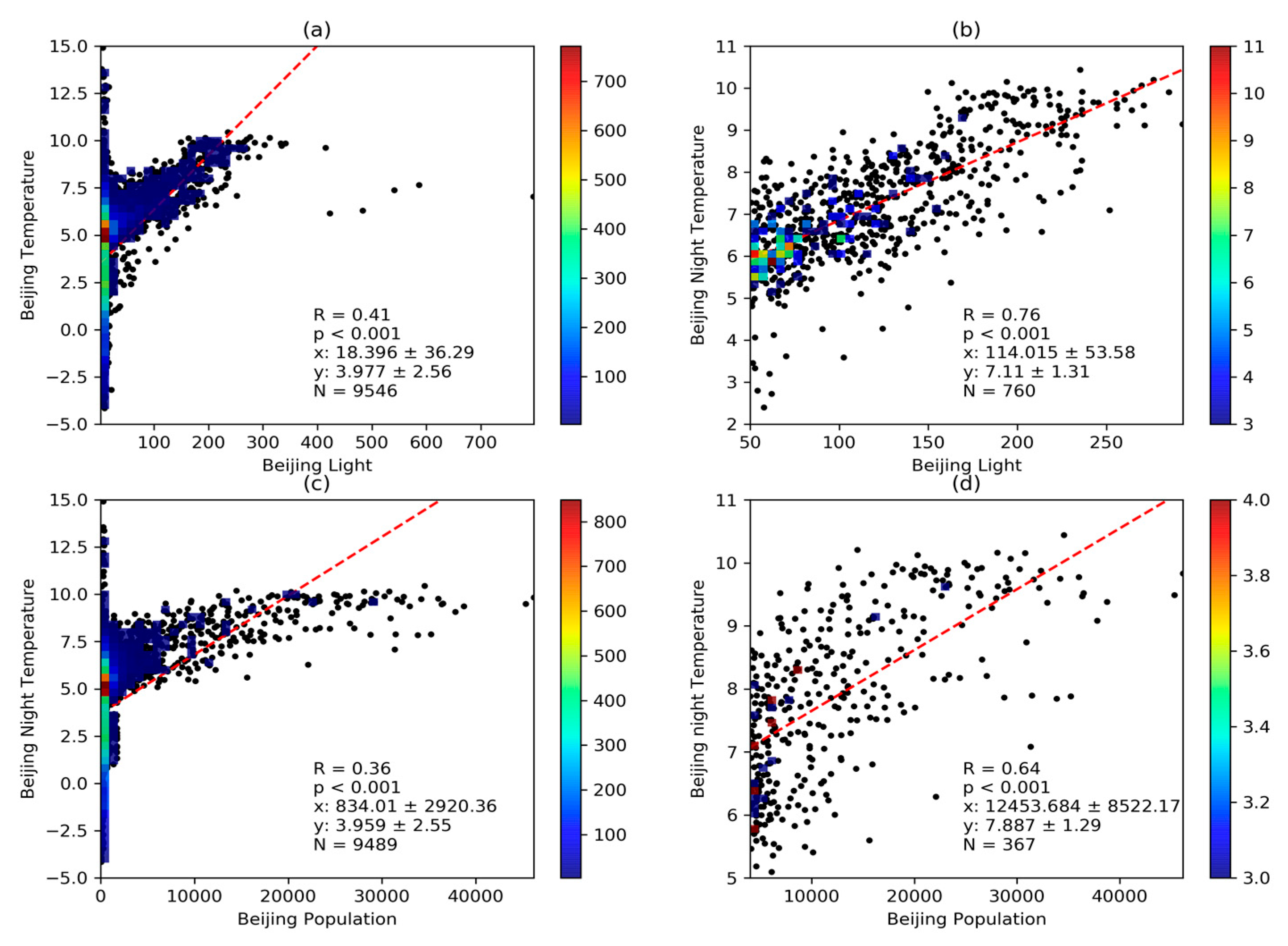
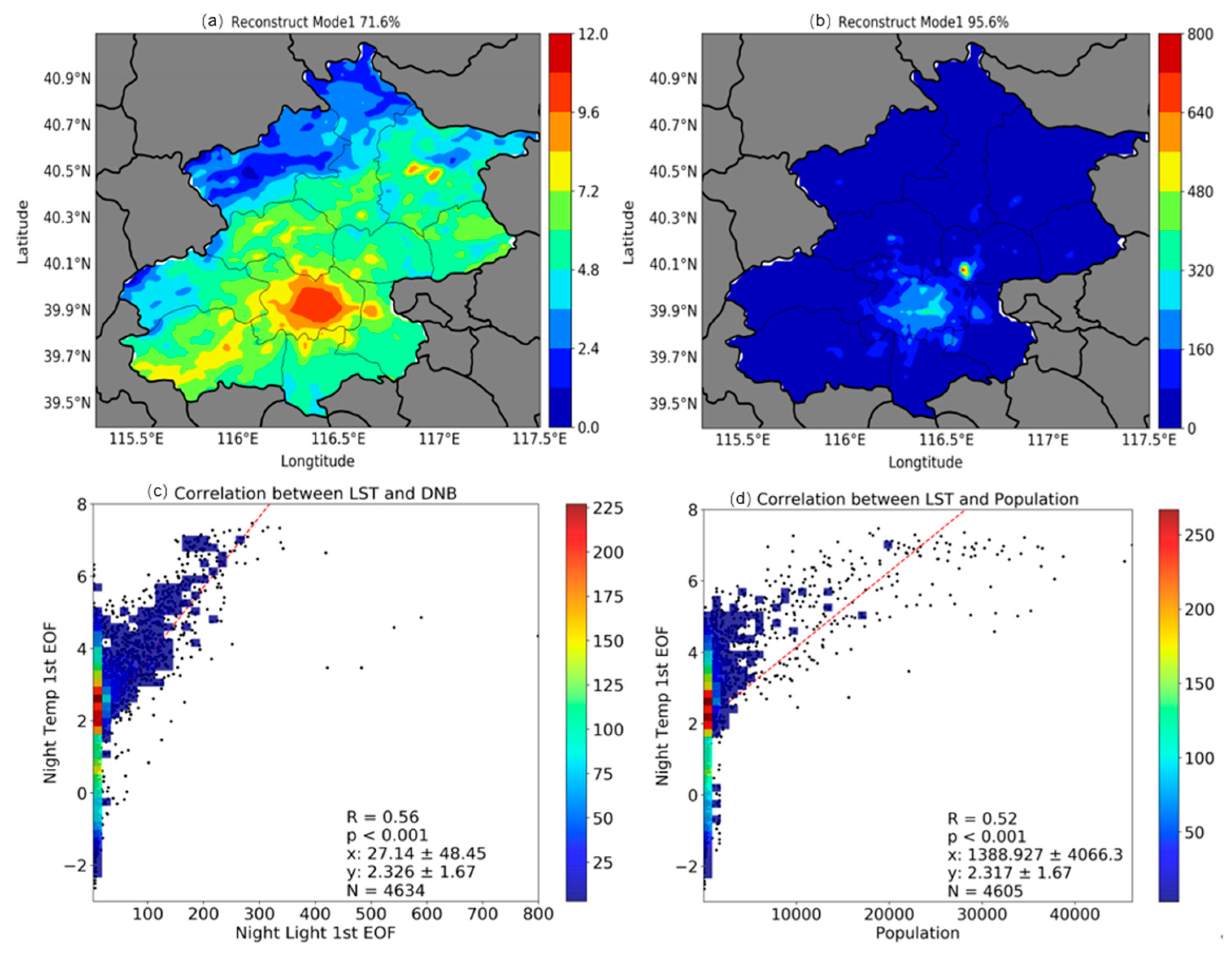
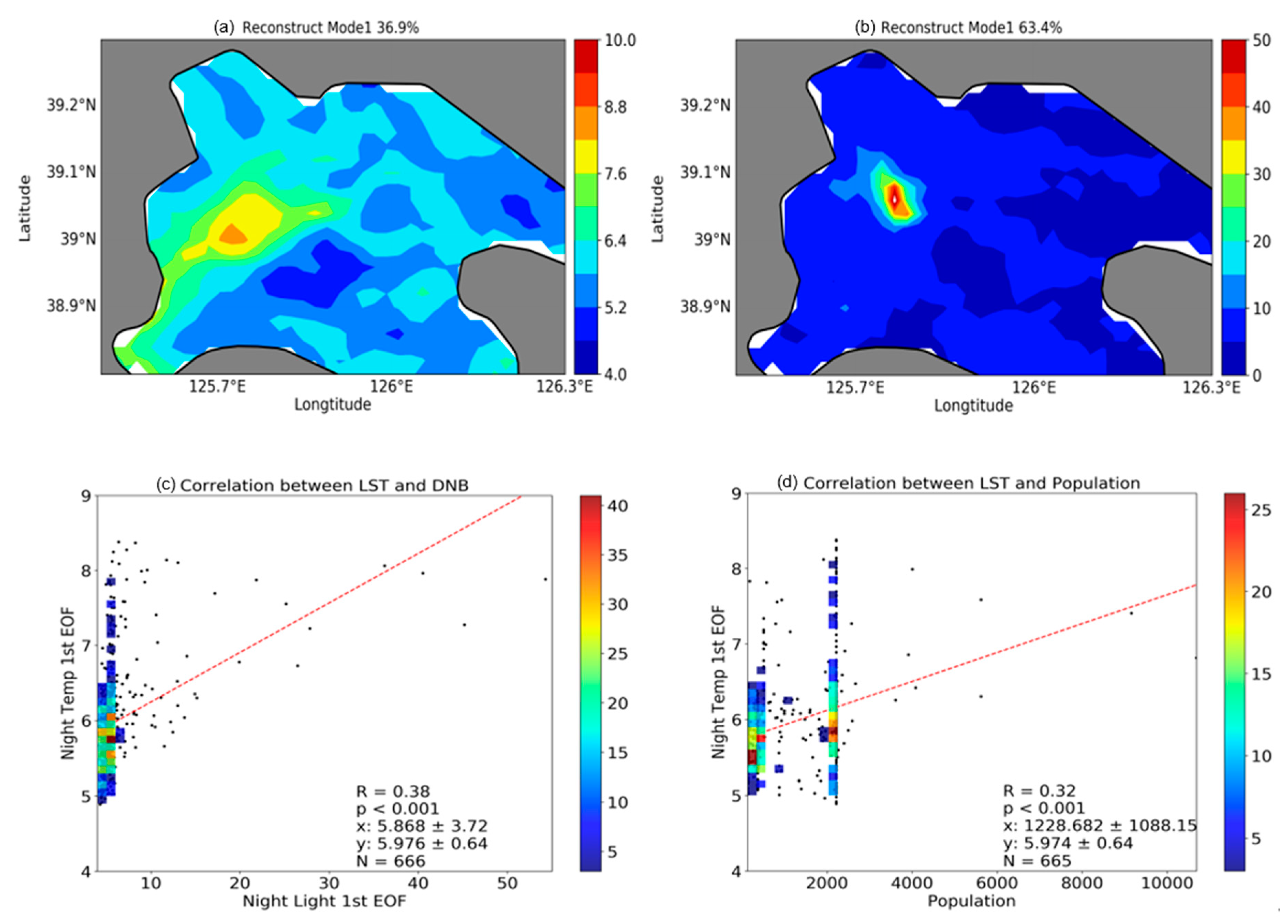
3.2. The Relationships between LST, DNB, and Population Data

DNB values at night can be a proxy for human activities and energy use at night, which may have a close relationship with nighttime LST. To test this hypothesis, nighttime LST data were used here to explore the correlations of LST with DNB intensity and population. The correlation between nighttime LST and nighttime DNB intensity in Beijing is shown in Figure 2a. Taking all of the grid boxes into consideration, their linear correlation coefficient is 0.41. Beijing is a city with many mountains in the northwest, where both nighttime temperature and night light are very low. In the meantime, there are also some pixels corresponding to high temperature but low night light, which lie in the southwest of Beijing and may have a relationship with the highways in this area. It is obvious that when the night light intensity is less than 50 nW/(cm²str), the distribution of the surface temperature is irregular, appearing as both low and high ground temperatures. After removing these outliers, pixels with night light intensity values larger than 50 nW/(cm²str) and smaller than 300 nW/(cm²str) were selected and are plotted in Figure 2b. It is obvious that the correlation coefficient between nighttime temperature and night light improves up to 0.76, with statistically significant p values being lower than 0.001. Population also correlates very highly with nighttime temperature. Similar to nightlight, it is evident that both higher and lower ground temperatures appear in areas with low population density. Figure 2c shows all pixels, with a correlation coefficient of 0.48, while Figure 2d shows pixels where the population density is larger than 4000 people per pixel, for which the correlation coefficient improves to 0.64; therefore, nighttime LST performs slightly better than population in describing the urban nighttime temperature in Beijing.

Similar to the analysis for Beijing, Figure 3 shows the linear correlation of LST with the DNB and population data in Pyongyang. Taking all pixels into consideration, the correlation coefficient between the LST and population data is lower than that between the LST and DNB data. After setting the threshold (light intensity values larger than 10 nW/(cm²str) and the population density is larger than 2000 people per pixel) to concentrate on urban centers, the correlation coefficient between the LST and DNB data increases to 0.51, while the correlation coefficient between the LST and population data decreases to 0.16; therefore, this high correlation contrast in Pyongyang also highlights the advantage of using DNB to study LST.

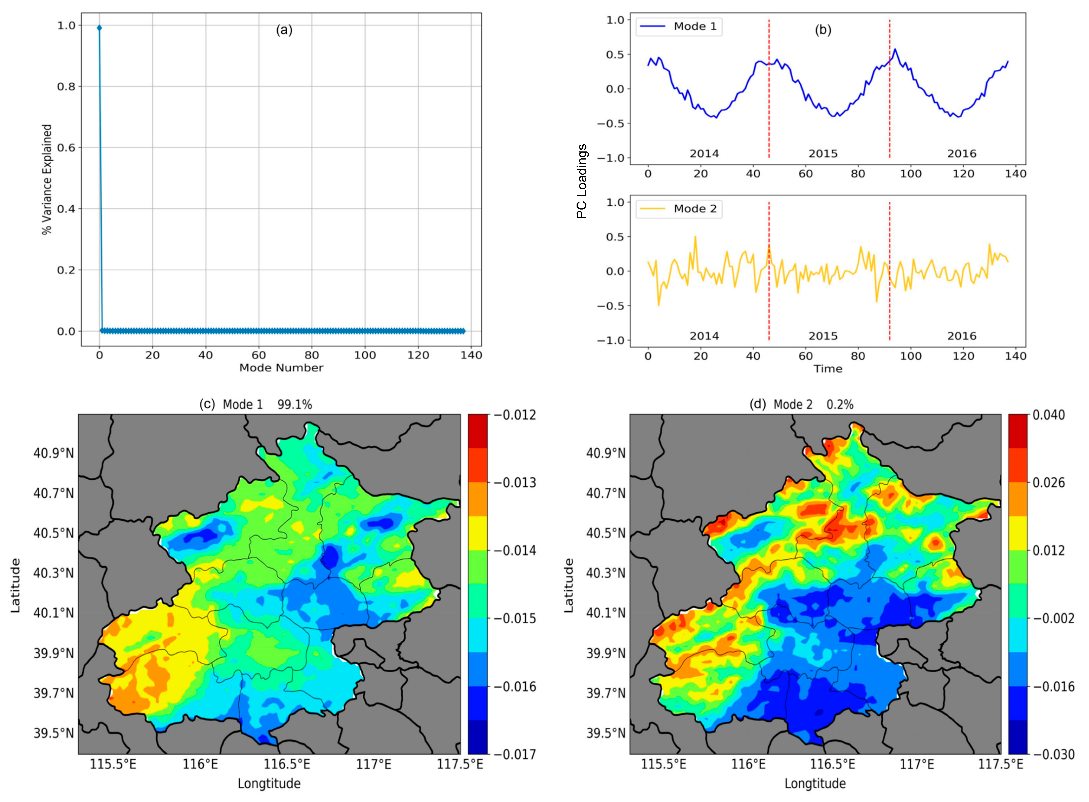
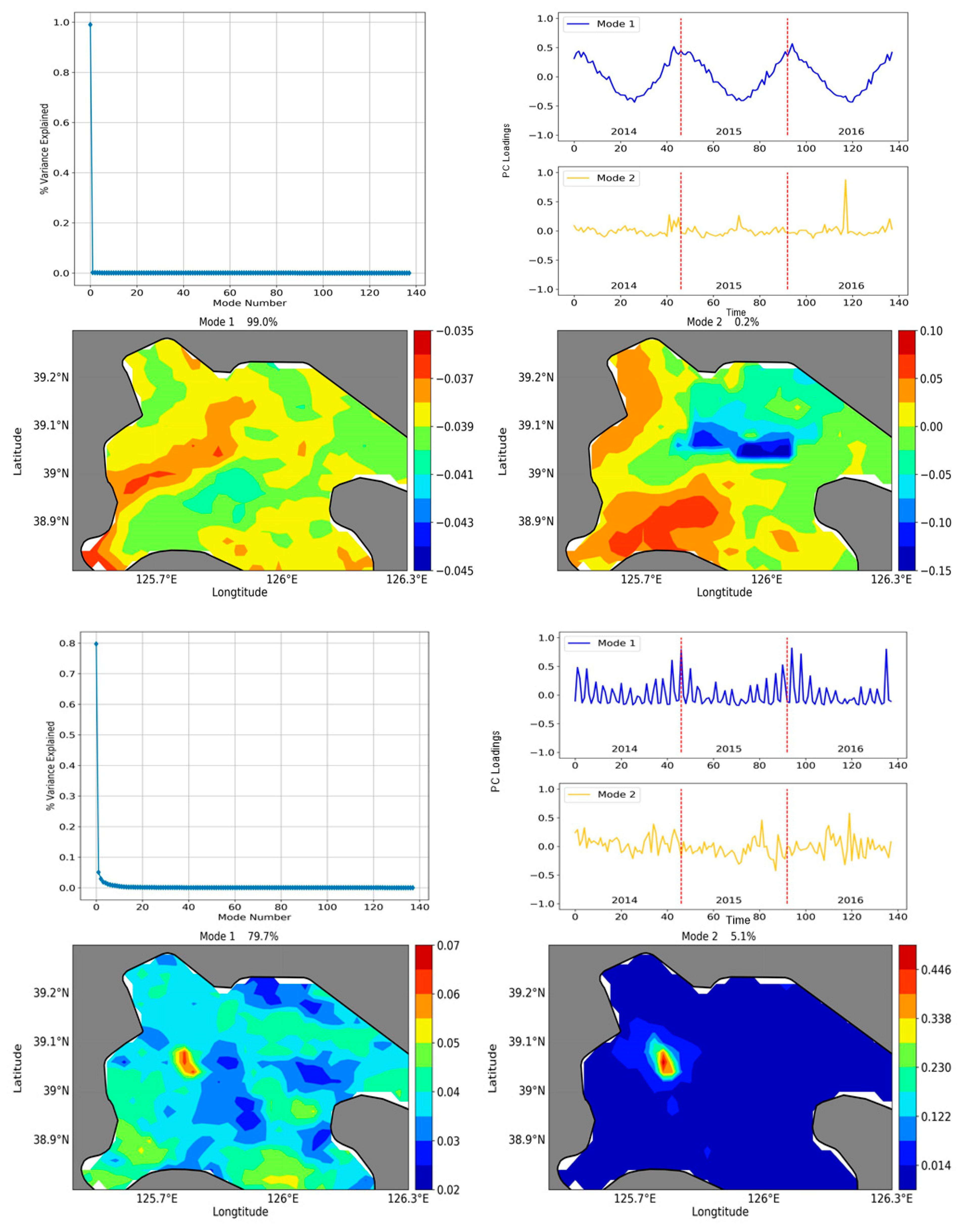
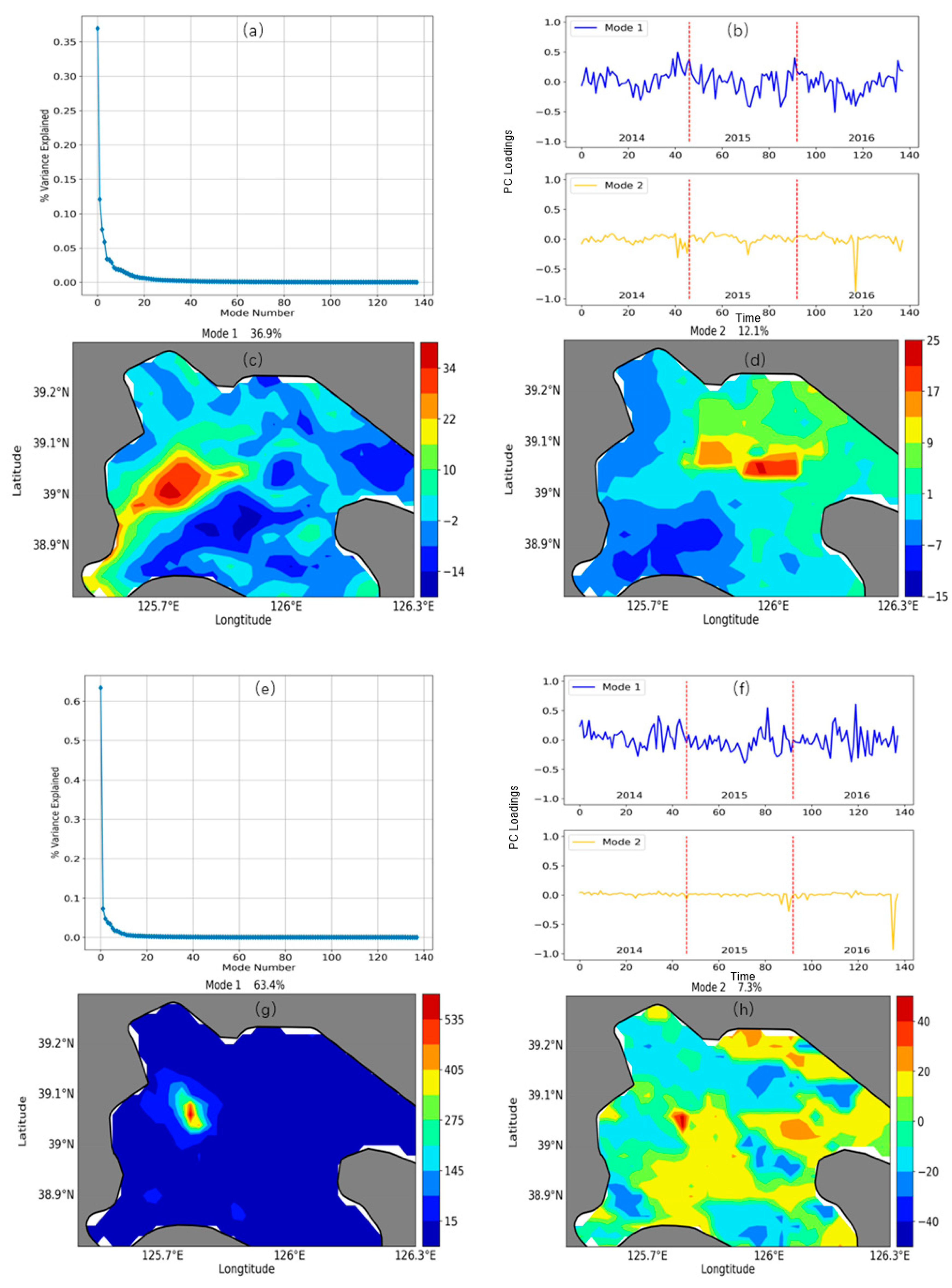
3.3. S-Mode PCA of Nighttime LST and DNB Data in Beijing and Pyongyang

LST and DNB data were analyzed by means of principal components analysis (PCA) in S-Mode (correlation between temporal series at each pixel) and in T-Mode (correlation between fields at each observation time). The two different kinds of analysis show how these approaches reveal different results. The results of the S-mode PCA are firstly presented in this section.

Figure 4 shows the S-mode PCA results for LST data. Figure 4a shows the explanation ratio for all PC loadings (PCLs), while Figure 4b shows the corresponding PC scores (PCS) for the first two PCLs. Figure 4c, d shows the spatial patterns for the first two PCLs. The PCL (PC loading) indicates the eigenvectors, while the PC score can be obtained by projecting the original data with respect to the corresponding PC loading. In other words, PCL is the main distribution of the variables under study and PCS is the changing curve corresponding to the distribution of the variable. The first PCL explains over 99% of the spatial variance, while the second PCL only explains 0.2%. PCS1 in Figure 4b shows an obvious seasonal cycle, and it was found that the deep blue areas located in Yanqing, Shunyi, and Daxing districts responded strongly to the seasonal cycle. The Beijing urban area responses were weaker, with the response for the mountainous area in northwest area being the weakest. There was no obvious cycle in PCS2. We can conclude that the seasonal cycle is the most representative main pattern for LST data. Figure 5 shows the S-mode PCA results for DNB data. The first PCL explains 75.7% of the variance, while the second explains only 5.5%. PCS1 shows an obvious seasonal cycle, while PCS2 shows a monthly cycle. Similar to the S-mode LST results, the seasonal cycle plays a dominant role in the S-mode DNB results. This may be related to the seasonal cycle of aerosol optical depths [39,40]. In addition, moonlight also has a great effect on the detection of the DNB, as presented in PCS2. There are about 12 peaks in each year. The S-mode results for LST and DNB data in Pyongyang are similar to those for Beijing (Figure 6). The first PCL explains over 99% of the variance and the time series shows a significant seasonal cycle. For DNB data, the first PCL reflects the natural variance of the moon phase. Comparing PCS1 from the DNB data in Beijing and Pyongyang, it is interesting that PCS1 for Pyongyang seems to be more regular than PCS1 of Beijing. It is suspected that this may have something to do with the different levels of pollution in the two cities.

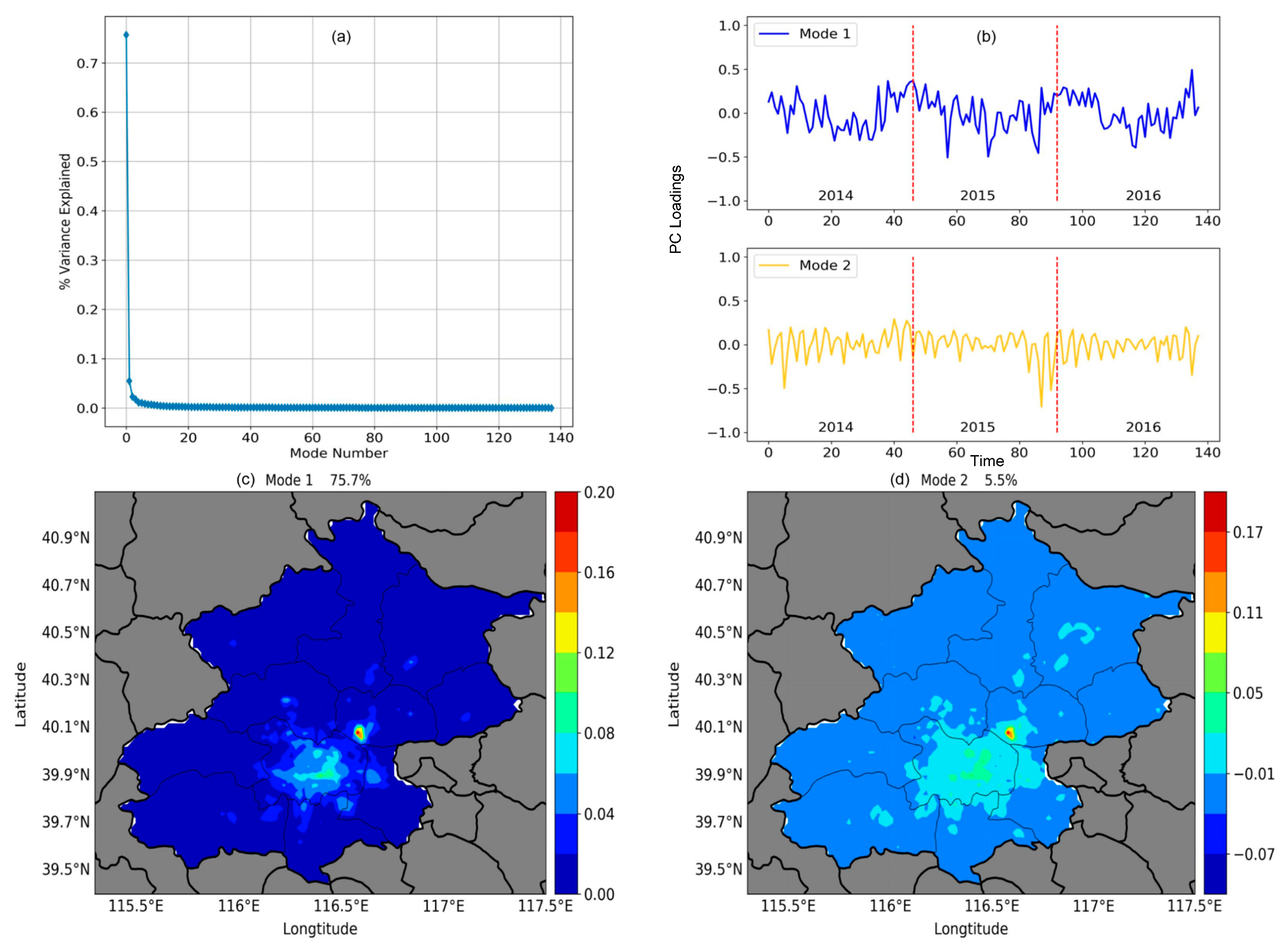
3.4. T-Mode PCA of Nighttime LST and DNB Data in Beijing and Pyongyang

LST temporal patterns can be described in terms of the significant PCLs in the T-mode PCA when focusing on the analysis of key features of the temporal variations of LST. The first two PCLs explained 81.6% of the total variance. Figure 7a shows the explanation ratio for each mode. The first LST pattern (PCL1) explains 71.6% of the total variance, while the second LST pattern (PCL2) explains 10.0%. Differing from Figure 4b, Figure 7b shows the first two PCLs, which characterize representative time series, while Figure 7c, d shows the distribution of the first PC scores. Figure 7c,d show the spatial patterns for PCL1 and PCL2, respectively. PCL1 shows that the largest value was located in the urban core, while lowest value appeared in the mountainous area of the city. PCL1 in Figure 7b shows an irregular fluctuation, showing that there is always an urban heat island pattern all year around when combined with the spatial pattern in Figure 7c. PCL2 shows a significant seasonal cycle and positive values mostly located in the mountainous areas, such as the Fangshan district in southwestern Beijing, while negative values are located in areas where human activities are frequent, such as Shunyi and Daxing districts in the northeastern and southern parts of Beijing, respectively. Combining Figure 7b,d demonstrates that when human activity is more active, the summer temperature increases more drastically. In addition, it is obvious that the variance in the urban core is very small in PCS2, which means that the urban core area is less sensitive to natural seasonal variance.

Figure 8 shows the PCA results for DNB data. The first PCL for DNB data explains 95.6% of the total variance, while the second PCL explains 0.5%. Figure 8b shows the first two PCLs, while Figure 8c and Figure 8d show the spatial patterns for PCL1 and PCL2, respectively. The largest value was located in Beijing airport and higher values appeared in the urban areas of this city, as shown in Figure 8c. The time series (PCL1) in Figure 8b shows a seasonal cycle, where DNB data are a little darker in summer, which may have been related to higher aerosol optical depths in summer. Che showed high AODs from June to August in Beijing, reflecting the hygroscopic growth of fine particles and the conversion of gases to particles over a broad area [41]. Furthermore, PCL2 shows a significant annual trend and positive signals mostly located in the airport area, while negative signals can be seen in areas where human activities are frequent. Combined with the PCL2 and PCS2, the deep blue spot indicates that DNB values are increasing in areas with frequent human activity and rapid development, such as Daxing, Shunyi, and Yanqing districts (the topographic map and DNB samples of Beijing are shown in Figure 1).

Since the explain ratios for LST and DNB data in mode 1 are all greater than 50%, the original can be reconstructed by multiplying the PCL and PCS in mode 1. The main characteristics of the original data can be more clearly reflected in the reconstructed data. Taking the first mode of LST and DNB data for reconstruction, we found that the correlation between reconstructed LST and DNB data was 0.56, which was improved a lot compared with the first value of 0.41 shown in Figure 3. This fully proves that the spatial patterns for LST and DNB data have high similarity. T-mode PCA can extract the majority of useful information. The correlation between reconstructed mode 1 LST and population data was also analyzed and the correlation coefficient was increased from 0.36 to 0.52 (Figure 9).

For Pyongyang in Figure 10, the T-mode PCA results for LST data show that there is a seasonal cycle and the hot areas are distributed in urban areas, as shown in PCS1. Simultaneously, there are some peaks in PCL2, which mostly happen in summer. These peaks may correspond to biomass burning. A seasonal cycle also exists in the PCL1 for T-mode PCA results for DNB data; however, there was no annual trend for DNB data, which means that we could not find an obvious developing signal for Pyongyang. Using PCL1 and PCS1 to reconstruct LST and DNB, the correlation coefficient between LST and DNB increased from 0.35 to 0.38. Similarly, the correlation of reconstructed LST and population data was also analyzed and the coefficient increased from 0.29 to 0.32 (Figure 11). To better illustrate the data processing and analysis, a structure diagram is shown in Figure 12.

4. Discussion

Beijing and Pyongyang are the capitals of China and North Korea, respectively. Beijing has undergone tremendous changes in the past 30 years and the speed of urbanization has been very fast. Pyongyang, on the other hand, has developed quite a lot slower than Beijing due to policy reasons. Nighttime lights are usually used to infer the accuracy of the official gross domestic product (GDP). This is because nighttime lights reflect real economic activities, meaning they are correlated with the true GDP. Beijing has a population of about 21.7 million and is one of the most urbanized and brightest cities in China on clear nights, while Pyongyang has a population of only 2.5 million. Human activities have significantly altered the distribution of nighttime surface temperatures. Areas with more human activity tend to have higher surface temperatures.

In this study, 8-day-interval nighttime LST data from Aqua, 750-m-resolution DNB data from the VIIRS, and gridded population data were used here to explore which factors can indicate the variations in nighttime LST. Linear correlation analysis showed that DNB has a closer correlation to nighttime LST data compared with population data. Because there was so much noise in the linear analysis, which reduced the correlation coefficient, PCA, a method used to extract main information, was used to investigate the relationships between LST, DNB, and population data. There are two types of PCA, namely S-mode PCA and T-mode PCA. Different types of PCA can lead to different results. S-mode PCA can obtain typical time series, while T-mode PCA achieves typical spatial patterns. The PCS1 results for LST in Beijing and Pyongyang showed significant seasonal cycles; however, the PCS1 results for DNB data in Beijing showed an obvious seasonal cycle, while PCS2 showed a monthly cycle, which may have been related to the moon phase. For Pyongyang, the PCS1 results for the DNB data reflected seasonal and monthly cycles at the same time, meaning the pollution level in Pyongyang is lower than in Beijing. T-mode PCA captured the spatial information well, whereby the first mode explained over 50% of the variance in both LST and DNB data. Using the first mode to reconstruct LST and DNB data for Beijing, we found that the correlation coefficient between reconstructed LST and DNB data increased from 0.41 in the linear analysis to 0.56. Furthermore, the correlation coefficient between reconstructed LST and population data increased from 0.36 in the linear analysis to 0.52. The same calculation was also applied in Pyongyang and the results showed that the correlation coefficient for reconstructed LST and DNB increased from 0.35 in the linear analysis to 0.38, while the correlation coefficient between reconstructed LST and population data increased from 0.29 in the linear analysis to 0.32. Combined with the second spatial pattern and time series for DNB data in Beijing, it was found that the districts where DNB values increased were built-up, with population levels also showing increasing trends. This fully demonstrates that DNB data are well suited for studying the spatial variation of urban heat islands, especially for nighttime urban temperatures taken from space, at the street and neighborhood scales.

The main contribution of this work was the use of the highest-resolution nighttime light data to explore the distribution of nighttime surface temperatures, meaning temperature data could be seen in more detail. Meanwhile, T-mode PCA and S-mode PCA were used for the first time to better analyze the temporal and spatial variations in nighttime light and nighttime surface temperature data, offering a new way to explore the urban heat island effect. In the past studies on urban heat, the population distribution has often been used; however, we show here that the light distribution can better reflect the spatial distribution of urban heat, as the population distribution cannot be tracked on a daily or monthly basis from space. The contrast between Beijing and Pyongyang was used here to highlight the value of using city light to study urban heat (rather than using population). Pyongyang has a sizeable population, although the economy is much less developed compared to Beijing. To our knowledge, this paper is among the first to use city light data in an analysis of urban heat distribution.

References

1. Peng, S.; Piao, S.; Ciais, P.; Friedlingstein, P.; Ottle, C.; Bréon, F.-M.; Nan, H.; Zhou, L.; Myneni, R.B. Surface Urban Heat Island Across 419 Global Big Cities. Environ. Sci. Technol. 2012, 46, 696–703. [Google Scholar] [CrossRef]
2. Zhou, D.; Zhao, S.; Liu, S.; Zhang, L.; Zhu, C. Surface urban heat island in China’s 32 major cities: Spatial patterns and drivers. Remote Sens. Environ. 2014, 152, 51–61. [Google Scholar] [CrossRef]
3. Arnfield, A.J. Two decades of urban climate research: A review of turbulence, exchanges of energy and water, and the urban heat island. Int. J. Climatol. 2003, 23, 1–26. [Google Scholar] [CrossRef]
4. Oke, T.R. City size and the urban heat island. Atmos. Environ. 1973, 7, 769–779. [Google Scholar] [CrossRef]
5. Voogt, J.A.; Oke, T.R. Thermal remote sensing of urban climates. Remote Sens. Environ. 2003, 86, 370–384. [Google Scholar] [CrossRef]
6. Dixon, P.G.; Mote, T.L. Patterns and Causes of Atlanta’s Urban Heat Island–Initiated Precipitation. J. Appl. Meteorol. 2003, 42, 1273–1284. [Google Scholar] [CrossRef]
7. Jin, M.; Dickinson, R.E.; Zhang, D. The Footprint of Urban Areas on Global Climate as Characterized by MODIS. J. Clim. 2005, 18, 1551–1565. [Google Scholar] [CrossRef]
8. Jin, M.; Shepherd, J.M.; King Michael, D. Urban aerosols and their variations with clouds and rainfall: A case study for New York and Houston. J. Geophys. Res. Atmos. 2005, 110, D10. [Google Scholar] [CrossRef]
9. Shepherd, J. A Review of Current Investigations of Urban-Induced Rainfall and Recommendations for the Future. Earth Interact. 2005, 9, 1–27. [Google Scholar] [CrossRef] [Green Version]
10. Gong, P.; Liang, S.; Carlton, E.J.; Jiang, Q.; Wu, J.; Wang, L.; Remais, J.V. Urbanisation and health in China. Lancet 2012, 379, 843–852. [Google Scholar] [CrossRef]
11. O’Loughlin, J.; Witmer, F.D.W.; Linke, A.M.; Laing, A.; Gettelman, A.; Dudhia, J. Climate variability and conflict risk in East Africa, 1990–2009. Proc. Natl. Acad. Sci. USA 2012, 109, 18344–18349. [Google Scholar] [CrossRef] [Green Version]
12. Patz, J.A.; Campbell-Lendrum, D.; Holloway, T.; Foley, J.A. Impact of regional climate change on human health. Nature 2005, 438, 310. [Google Scholar] [CrossRef] [PubMed]
13. McCarthy Mark, P.; Best Martin, J.; Betts Richard, A. Climate change in cities due to global warming and urban effects. Geophys. Res. Lett. 2010, 37. [Google Scholar] [CrossRef] [Green Version]
14. Imhoff, M.L.; Zhang, P.; Wolfe, R.E.; Bounoua, L. Remote sensing of the urban heat island effect across biomes in the continental USA. Remote Sens. Environ. 2010, 114, 504–513. [Google Scholar] [CrossRef] [Green Version]
15. Jin, M.; Shepherd, J.M.; Zheng, W. Urban Surface Temperature Reduction via the Urban Aerosol Direct Effect: A Remote Sensing and WRF Model Sensitivity Study. Adv. Meteorol. 2010, 2010, 1–14. [Google Scholar] [CrossRef] [Green Version]
16. Gallo, K.P.; McNab, A.L.; Karl, T.R.; Brown, J.F.; Hood, J.J.; Tarpley, J.D. The Use of NOAA AVHRR Data for Assessment of the Urban Heat Island Effect. J. Appl. Meteorol. 1993, 32, 899–908. [Google Scholar] [CrossRef] [Green Version]
17. Huang, J.; Lin, B.; Minnis, P.; Wang, T.; Wang, X.; Hu, Y.; Yi, Y.; Ayers, J.K. Satellite-based assessment of possible dust aerosols semi-direct effect on cloud water path over East Asia. Geophys. Res. Lett. 2006, 33, L19802. [Google Scholar] [CrossRef] [Green Version]
18. Zhang, Q.; Schaaf, C.; Seto, K.C. The Vegetation Adjusted NTL Urban Index: A new approach to reduce saturation and increase variation in nighttime luminosity. Remote Sens. Environ. 2013, 129, 32–41. [Google Scholar] [CrossRef]
19. Elvidge, C.D.; Baugh, K.; Zhizhin, M.; Hsu, F.C.; Ghosh, T. VIIRS night-time lights. Int. J. Remote Sens. 2017, 38, 5860–5879. [Google Scholar] [CrossRef]
20. Cao, C.; Lee, X.; Liu, S.; Schultz, N.; Xiao, W.; Zhang, M.; Zhao, L. Urban heat islands in China enhanced by haze pollution. Nat. Commun. 2016, 7, 12509. [Google Scholar] [CrossRef]
21. Karl, T.R.; Diaz, H.F.; Kukla, G. Urbanization: Its Detection and Effect in the United States Climate Record. J. Clim. 1988, 1, 1099–1123. [Google Scholar] [CrossRef] [Green Version]
22. Oke, T.R. The energetic basis of the urban heat island. Q. J. R. Meteorol. Soc. 1982, 108, 1–24. [Google Scholar] [CrossRef]
23. Tran, H.; Uchihama, D.; Ochi, S.; Yasuoka, Y. Assessment with satellite data of the urban heat island effects in Asian mega cities. Int. J. Appl. Earth Obs. Geoinf. 2006, 8, 34–48. [Google Scholar] [CrossRef]
24. Zhao, L.; Lee, X.; Smith, R.B.; Oleson, K. Strong contributions of local background climate to urban heat islands. Nature 2014, 511, 216. [Google Scholar] [CrossRef]
25. Levin, N.; Zhang, Q. A global analysis of factors controlling VIIRS nighttime light levels from densely populated areas. Remote Sens. Environ. 2017, 190, 366–382. [Google Scholar] [CrossRef] [Green Version]
26. Elvidge, C.D. Mapping City Lights with Nighttime Data from the DMSP Operational Linescan System, Photogramm. Eng. Remote Sens. 1997, 63, 727–734. [Google Scholar]
27. Yan, Z.; Li, Z.; Li, Q.; Jones, P. Effects of site change and urbanisation in the Beijing temperature series 1977–2006. Int. J. Climatol. 2009, 30, 1226–1234. [Google Scholar] [CrossRef]
28. Zhengming, W.; Dozier, J. A generalized split-window algorithm for retrieving land-surface temperature from space. IEEE Trans. Geosci. Remote Sens. 1996, 34, 892–905. [Google Scholar] [CrossRef] [Green Version]
29. Wan, Z. New refinements and validation of the MODIS Land-Surface Temperature/Emissivity products. Remote Sens. Environ. 2008, 112, 59–74. [Google Scholar] [CrossRef]
30. Rigo, G.; Parlow, E.; Oesch, D. Validation of satellite observed thermal emission with in-situ measurements over an urban surface. Remote Sens. Environ. 2006, 104, 201–210. [Google Scholar] [CrossRef]
31. Miller, S.D.; Mills, S.P.; Elvidge, C.D.; Lindsey, D.T.; Lee, T.F.; Hawkins, J.D. Suomi satellite brings to light a unique frontier of nighttime environmental sensing capabilities. Proc. Natl. Acad. Sci. USA 2012, 109, 15706. [Google Scholar] [CrossRef] [Green Version]
32. Miller, D.S.; Straka, W.; Mills, P.S.; Elvidge, D.C.; Lee, F.T.; Solbrig, J.; Walther, A.; Heidinger, K.A.; Weiss, C.S. Illuminating the Capabilities of the Suomi National Polar-Orbiting Partnership (NPP) Visible Infrared Imaging Radiometer Suite (VIIRS) Day/Night Band. Remote Sens. 2013, 5, 6717–6766. [Google Scholar] [CrossRef] [Green Version]
33. Socioeconomic Data and Applications Center. Gridded Population of the World, Version 4 (GPWv4): Population Density, Revision 10; NASA Socioeconomic Data and Applications Center (SEDAC): Palisades, NY, USA, 2017.
34. Pearson, K. LIII. On lines and planes of closest fit to systems of points in space. Lond. Edinb. Dublin Philos. Mag. J. Sci. 1901, 2, 559–572. [Google Scholar] [CrossRef] [Green Version]
35. Li, J.; Carlson, B.E.; Lacis, A.A. Application of spectral analysis techniques in the intercomparison of aerosol data: Part III. Using combined PCA to compare spatiotemporal variability of MODIS, MISR, and OMI aerosol optical depth. J. Geophys. Res. Atmos. 2013, 119, 4017–4042. [Google Scholar] [CrossRef] [Green Version]
36. Li, J.; Carlson, B.E.; Lacis, A.A. Application of spectral analysis techniques in the intercomparison of aerosol data: 1. An EOF approach to analyze the spatial-temporal variability of aerosol optical depth using multiple remote sensing data sets. J. Geophys. Res. Atmos. 2013, 118, 8640–8648. [Google Scholar] [CrossRef]
37. Barreira, S.; Compagnucci, R.H. Spatial fields of Antarctic sea-ice concentration anomalies for summer–autumn and their relationship to Southern Hemisphere atmospheric circulation during the period 1979–2009. Ann. Glaciol. 2011, 52, 140–150. [Google Scholar] [CrossRef] [Green Version]
38. Compagnucci, R.H.; Richman, M.B. Can principal component analysis provide atmospheric circulation or teleconnection patterns? Int. J. Climatol. 2007, 28, 703–726. [Google Scholar] [CrossRef]
39. Song, Z.; Fu, D.; Zhang, X.; Wu, Y.; Xia, X.; He, J.; Han, X.; Zhang, R.; Che, H. Diurnal and seasonal variability of PM2.5 and AOD in North China plain: Comparison of MERRA-2 products and ground measurements. Atmos. Environ. 2018, 191, 70–78. [Google Scholar] [CrossRef]
40. Wang, J.; Aegerter, C.; Xu, X.; Szykman, J.J. Potential application of VIIRS Day/Night Band for monitoring nighttime surface PM2.5 air quality from space. Atmos. Environ. 2016, 124, 55–63. [Google Scholar] [CrossRef] [Green Version]
41. Che, H.; Zhang, X.Y.; Xia, X. Ground-based aerosol climatology of China: Aerosol optical depths from the China Aerosol Remote Sensing Network (CARSNET) 2002–2013. Atmos. Chem. Phys. 2015, 15, 7619–7652. [Google Scholar] [CrossRef] [Green Version]
Figure 1. The elevation map (a), spatial distribution of averaged nighttime LSTs for 2014–2016 (b), visible light intensity (c), and population data (d) for Beijing, the same aspects are shown for Pyongyang (eh), (i) is the administrative map. The red box indicates Beijing Capital Airport.
Remotesensing 13 03180 g001
Figure 2. The correlation between the nighttime LST and night light (a), the correlation between the nighttime LST and annual mean population over 5 years based on all data (c), (b,d) are the density distribution for all night light values ranging between 50 and 300 nW/(cm2str) and with a population level larger than 4000 per pixel in Beijing.
Remotesensing 13 03180 g002
Figure 3. Same as Figure 2 but for Pyongyang. The correlation between the nighttime LST and night light (a), the correlation between the nighttime LST and annual mean population over 5 years based on all data (c), (b,d) are the density distribution for all night light values larger than 10 nW/(cm2str) and with a population level larger than 2000 per pixel.
Remotesensing 13 03180 g003
Figure 4. The S-mode PCA results for Beijing surface temperature data during 2014–2016: (a) the variance explained by the principal covariance analysis (PCA) modes for surface temperature; (b) the PC time series of the first two modes (the red vertical lines are used to divide data into different years); (c,d) the spatial patterns of the first two modes for the PCA results.
Remotesensing 13 03180 g004
Figure 5. The S-mode PCA results for Beijing DNB data during 2014–2016: (a) the variance explained by the principal covariance analysis (PCA) modes for DNB; (b) the PC time series for the first two modes (the red vertical lines are used to divide data in different years); (c,d) the spatial patterns of the first two modes for the PCA results.
Remotesensing 13 03180 g005
Figure 6. The S-mode PCA results for LST and DNB data in Pyongyang. The first four panels show the LST results and the last four panels show DNB results.
Remotesensing 13 03180 g006
Figure 7. The T-mode PCA results for Beijing surface temperature data during 2014–2016: (a) the variance explained by the principal covariance analysis (PCA) modes for surface temperature; (b) the PC time series for the first two modes (the red vertical lines are used to divide data into different years); (c,d) the spatial patterns of the first two modes for PCA results.
Remotesensing 13 03180 g007
Figure 8. The T-mode PCA results for Beijing DNB data during 2014–2016, (a) the variance explained by the principal covariance analysis (PCA) modes for surface temperatures, (b) the PC time series for the first two modes (the red vertical lines are used to divide data into different years, (c,d) the spatial patterns of the first two modes for PCA results.
Remotesensing 13 03180 g008
Figure 9. The reconstructed mode 1 LST and DNB datasets and the correlation between them in Beijing, (a) the spatial distribution of the reconstructed mode 1 LST and (b) DNB datasets, (c) the correlation between the reconstructed LST and DNB datasets using mode 1, (d) the correlation between reconstructed LST and original population data.
Remotesensing 13 03180 g009
Figure 10. The T-mode PCA results for Pyongyang LST (the first four panels) and DNB (the last four panels) data during 2014–2016. (a) the variance explained by the principal covariance analysis (PCA) modes for LST, (b) the PC time series for the first two modes of LST (the red vertical lines are used to divide data into different years, (c,d) the spatial patterns of the first two modes for LST PCA results, (e) the variance explained by the principal covariance analysis (PCA) modes for DNB, (f) the PC time series for the first two modes of DNB, (g,h) the spatial patterns of the first two modes for the DNB PCA results.
Remotesensing 13 03180 g010
Figure 11. The reconstructed mode 1 LST and DNB datasets and the correlation between them in Pyongyang: (a) the spatial distribution of the reconstruct mode 1 LST and (b) DNB datasets; (c) the correlation between reconstructed LST and DNB datasets using mode 1; (d) is the correlation between reconstructed LST and original population data.
Remotesensing 13 03180 g011
Figure 12. The structure diagram of the data processing and analysis.
Remotesensing 13 03180 g012
Publisher’s Note: MDPI stays neutral with regard to jurisdictional claims in published maps and institutional affiliations.