Performance Evaluation of Long NDVI Timeseries from AVHRR, MODIS and Landsat Sensors over Landslide-Prone Locations in Qinghai-Tibetan Plateau

Abstract

The existence of several NDVI products in Qinghai-Tibetan Plateau (QTP) makes it challenging to identify the ideal sensor for vegetation monitoring as an important factor for landslide detection studies. A pixel-based analysis of the NDVI time series was carried out to compare the performances of five NDVI products, including ETM+, OLI, MODIS Series, and AVHRR sensors in QTP. Harmonic analysis of time series and wavelet threshold denoising were used for reconstruction and denoising of the five NDVI datasets. Each sensor performance was assessed based on the behavioral similarity between the original and denoised NDVI time series, considering the preservation of the original shape and time series values by computing correlation coefficient (CC), mean absolute error (MAE), root mean square error (RMSE), and signal to noise ratio (SNR). Results indicated that the OLI slightly outperformed the other sensors in all performance metrics, especially in mosaic natural vegetation, grassland, and cropland, providing 0.973, 0.015, 0.022, and 27.220 in CC, MAE, RMSE, and SNR, respectively. AVHRR showed similar results to OLI, with the best results in the predominant type of land covers (needle-leaved, evergreen, closed to open). The MODIS series performs lower across all vegetation classes than the other sensors, which might be related to the higher number of artifacts observed in the original data. In addition to the satellite sensor comparison, the proposed analysis demonstrated the effectiveness and reliability of the implemented methodology for reconstructing and denoising different NDVI time series, indicating its suitability for long-term trend analysis of different natural land cover classes, vegetation monitoring, and change detection.

1. Introduction

The most extensive plateau in the world, the Qinghai-Tibetan Plateau (QTP), is covered with a broad range of vegetation from forests to shrublands [1], which are spatially distributed [2] and play an essential role in controlling the amount of transpiration and albedo, and thus, adjusting the energy balance between the surface and atmosphere [3,4]. Furthermore, the southern QTP (especially the Himalayan region and its surrounding areas) is a famous landslide hotspots region at a global scale, with hundreds to thousands of deaths each year [5,6,7,8,9,10,11]. The spatiotemporal analysis of landslide events requires vast knowledge about static and dynamic landslide conditioning factors (LCFs), chiefly surface topography factor; elevation, curvature, distance to faults, geology, slope, hydrologic factor; distance to road, stream power index (SPI), topographic, witness index (TWI), rainfall, and vegetation cover factor; and NDVI [12,13,14,15]. Among these, vegetation is considered as a prominent dynamic factor playing an important role in landslide studies [16], as landslides can be detected by analyzing temporal changes in vegetation covers [17]. Vegetation, combined with tectonic, climate, and human factors, caused frequent and serious landslide disasters in the region [18,19,20,21,22]. The monitoring and analysis of vegetation dynamics, including its structure changes and spatiotemporal patterns, is requested for the landslide studies at regional and local scales in QTP [23,24].

The QTP is an ideal region for monitoring long-term vegetation dynamics due to its unique physiographical situation, vegetation distribution, climate, and relatively lesser human interference. However, the limited observed data has hindered knowledge about the vegetation dynamics and environmental conditions in QTP in the past. In recent decades, with the development of multi-temporal optical remote sensing with broad area coverage, the ability to continuously monitor vegetation dynamics has improved dramatically. Systematic time-series analysis of multi-temporal satellite observations can promote the exploration of vegetation variations and its changes that significantly impact the environments [25,26,27,28,29,30] and especially the manifestations of natural disasters (such as landslides, snow, etc.) in QTP [31,32].

The spatiotemporal characteristics of vegetation dynamics are continuously monitored through various vegetation indices (VIs), including normalized difference vegetation index (NDVI), leaf area index (LAI), enhanced vegetation index (EVI), and modified soil adjusted vegetation index (MSAVI) [33]. The reliable and straightforward VIs are usually obtained from multi-temporal resolution imageries of the fundamental optical properties of vegetation utterly absorbed in the red but highly reflective in near-infrared (NIR) regions [34,35]. Among all VIs, NDVI is widely used to monitor and characterize vegetation dynamics and their large-scale spatial variations due to its sensitivity to the vegetation cover, vegetation types, and productivity [35,36,37,38]. In particular, the application of NDVI is of utmost importance in those areas with sparse vegetation for monitoring vegetation dynamics [39,40,41].

Recently, many studies (Table 1) have used the NDVI time series in QTP for various purposes, including climate change, net primary production, landcover classification, greening and browning, land surface temperature, natural disasters, and human activity, etc. In these studies, multi-temporal satellite imageries with different spatial resolutions (MODIS 250–500m, AVHRR 1km, SPOT 1km, and Landsat series 30m) were used, and their results overall indicate a positive trend of plant growth and increased growing season, especially for alpine grasslands in QTP. A positive relationship between temperature and inter-annual variation of vegetation growth has been reported, with some differences among diverse vegetation types. However, the results of NDVI time series analysis vary with the different NDVI products used, leading to uncertainties and inconsistencies in deciphering vegetation dynamics in QTP [42,43,44]. Moreover, the results may differ due to the different methods used or differences in pixel sizes in different studies [3]. The heterogeneity in spatiotemporal factors further leads to inconsistencies in the NDVI analysis in QTP [33].

Additionally, cloud contamination due to structural complexity (high altitude), water vapor transport, and convective weather conditions is a recurring phenomenon in the NDVI dataset in QTP [45]. The NDVI datasets obtained from different acquisition conditions (multi-temporal satellite observatories) may be associated with multiple sources of inconsistencies including sensor shifts, degradation, seasonal snow, observational geometry inconsistencies (systematic and inherent noise), and ground conditions [46,47,48,49,50,51]. These lead to interruption, loss (missing), or contamination of the NDVI time series due to noise, leading to the inconsistency of NDVI products in QTP. Extensive attempts have been made to reduce noise, gaps, and determine NDVI patterns in QTP on various sensors (MODIS, AVHRR, Landsat, etc.), mainly using spectral frequency methods such as Fourier transform (FT), harmonic analysis of time series (HANTS), and wavelet threshold denoising (WTD) [45,52,53]. However, these studies were limited to specific sensors or NDVI product performance in specific vegetation types (alpine grassland as the predominant vegetation type).

Although individual sensors performance for spatiotemporal monitoring of vegetation dynamics in QTP has been extensively studied, NDVI time series analysis combined with a comparison of multiple satellite sensor modeling performances in different land covers in QTP has received less attention. Therefore, a comprehensive performance comparison between different satellites is essential to identify and illuminate the best satellite product for long-time NDVI time series analysis in the region, especially for landslide-susceptible locations, as an essential basis for the environment and natural disasters (landslide) studies. To fill the existing gap, this study aims explicitly at the pixel-based comparison of the robustness of long NDVI time series derived from five satellite sensors (AVHRR, MOD, MYD, EMT+, and OLI) in the different land covers of the landslide-prone locations in the QTP region during 2000–2020, differing from previous studies only focused on a specific part of the region and on a specific sensor. Identifying the best sensor performance offers an excellent tool for temporal vegetation monitoring and provides an essential and unique baseline for future landslide studies, especially landslide modeling (spatial and temporal) in the region, which requires accurate information from dynamic conditioning factors such as NDVI. Moreover, considering that the NDVI datasets are inherently noisy and contain missing values, we use the two state-of-the-art algorithms, including HANTS for the reconstruction (gap-filling) and the wavelet threshold denoising (WTD) for denoising (smoothing, reducing the noise interference, and data inconsistency) and modeling purposes. The performance assessment was based on the capability of the observed and denoised NDVI time series to preserve the structure of the original shape and time series values. The specific objectives of this study are:

i.

Evaluation of the performances of the five NDVI datasets in different land covers as well as over the predominant land cover types in QTP;

ii.

Identification of the most suitable sensor for NDVI time series analysis across QTP.

Table 1. Summary of relevant NDVI time series analysis studies using different NDVI products in the Qinghai-Tibetan Plateau (QTP).

No	Topics of NDVI Application	NDVI-Product (Sensor)/Period of Study	Key Findings	Reference
1	NDVI (Grassland phenology) and climate change relationship	GIMMS NOAA-AVHRR (15-day composite) (1982–2006)	NDVI significantly related to increasing temperatures, precipitation effects less pronounced.	[44]
2	NPP of Alpine Grassland; effect of topography and human activity	NOAA-AVHRR (10-day composite) MODIS (10-day composite) (1981–2004)	NPP (Net Primary Productivity) showed greater decreasing trend in high-elevation regions with slope 15–30°, aspect having little influence and roads having higher effect than residential areas.	[54]
3	Grassland vegetation cover and climatic factors	GIMMS NOAA-AVHRR (15-day composite) (1982–1999)	NDVI increase in growing season from both advanced growing season and accelerated vegetation activity. Apart from temperate steppe, NDVI exhibited no significant increase in autumn, corresponded to an increase in temperature in spring, and in summer, it was related to temperature and sensitive to precipitation in the spring. There were significant lagged correlations between precipitation and NDVI for alpine grasslands (alpine meadow, alpine steppe).	[55]
4	Vegetation greening and elevation	SPOT-VGT (10-day maximum value composite) (1999–2013)	NDVI increased more at lower elevations, but was relatively stable or even decreased at high elevations. Vegetation greening rate is in contrast to the pattern of elevation-dependent warming (EDW) with more significant temperature increases at higher elevations. Decreasing precipitation does not reverse overall increasing trend in NDVI, but it may be a limiting factor.	[56]
5	Vegetation response to temperature changes	GIMMS NOAA-AVHRR (15-day composite) (1981–1999)	Persistent increase in growing season NDVI and longer active growing season brought about by an early spring and delayed autumn. NDVI decreases possibly due to temperature-induced drought. Meaningful relation between changes in NDVI and land surface temperature.	[30]
6	Human impact on vegetation dynamics	SPOT-VGT (10-day maximum value composite) (1999–2013)	Impact of human activities in a relatively large area is minor and does not reverse the major trends of vegetation dynamics caused by the warming temperature in recent decades.	[25]
7	Spatial pattern of soil respiration in Tibetan alpine grasslands	Landsat TM MODIS (8-day composite) (2006)	NDVI exhibits spatial variation in soil respiration better than EVI and MSAVI. At the peak growing season of alpine grasslands, soil respiration was generally much higher in the SE Tibetan Plateau and gradually decreased toward NW part.	[57]
8	Monitoring vegetation phenology in Tibetan alpine grasslands	MODIS (16-day composite) C5 and C6 (2001–2015)	To evaluate the uncertainty of MODIS C5 and C6 NDVI in monitoring vegetation phenology, higher resolution near-surface remote sensing data and corresponding validation methods needed.	[29]
9	Vegetation classification	MODIS (16-day composite) (2004)	NDVI time-series curves of coniferous forest, high-cold meadow, high-cold meadow steppe and high-cold steppe all appear a mono-peak model during vegetation growth with the maximum peak occurring in August.	[58]
10	Sensitivity of NDVI to climate conditions	NOAA AVHRR GVI (1985–1999)	NDVI time series shows increasing trend of vegetation biomass. NDVI is strongly correlated but more sensitive to precipitation than temperature in semiarid climate zone of Lhasa area.	[59]
11	Variation in NPP	GIMMS NOAA-AVHRR (15-day composite) (1982–1999)	NPP decreases from the SE to the NW TP, consistent with precipitation and temperature patterns. NPP trends for most vegetation types resembled that of the whole plateau with alpine meadows showing the largest annual NPP increase. Changes in solar radiation and temperature significantly influenced NPP variation.	[60]
12	Vegetation and climate change	GIMMS NOAA-AVHRR (15-day composite) (1982–2012)	NDVI and temperature positively correlated during the growing season, responses to changes in precipitation were complex, particularly for different vegetation types. Growing season NDVI increased in 55% area of TP.	[27]
13	Vegetation trend	Landsat 5, 7, and 8 MODIS (16-day composite) (1990–2018)	Vegetation trend (NDVI product) for the entire Tibetan Plateau at 30 m spatial resolution for 1990–2018.	[3]
14	Green-up dates or Start of vegetation growing season (SOS)	GIMMS NOAA-AVHRR (15-day composite) SPOT VGT (10-day composite) MODIS (16-day composite) (1982–2011)	GIMMS NDVI in 2001–2006 differed substantially from SPOT-VGT and MODIS NDVIs and may have severe data quality issues in western TP. Alpine vegetation SOS in experienced continuous advancing trend in 1982–2011, consistent with observed warming in springs and winters.	[61]
15	Start of vegetation growing season (SGS)	GIMMS NOAA-AVHRR (15-day composite) SPOT VGT (10-day composite) (1982–2012)	SGS values display advancing trend with significant variations in SGS dates related to vegetation cover. Critical to know seasonal change characteristics of the different vegetation types, particularly in areas with sparse grassland or evergreen forest.	[53]

Table 1. Summary of relevant NDVI time series analysis studies using different NDVI products in the Qinghai-Tibetan Plateau (QTP).

No	Topics of NDVI Application	NDVI-Product (Sensor)/Period of Study	Key Findings	Reference
1	NDVI (Grassland phenology) and climate change relationship	GIMMS NOAA-AVHRR (15-day composite) (1982–2006)	NDVI significantly related to increasing temperatures, precipitation effects less pronounced.	[44]
2	NPP of Alpine Grassland; effect of topography and human activity	NOAA-AVHRR (10-day composite) MODIS (10-day composite) (1981–2004)	NPP (Net Primary Productivity) showed greater decreasing trend in high-elevation regions with slope 15–30°, aspect having little influence and roads having higher effect than residential areas.	[54]
3	Grassland vegetation cover and climatic factors	GIMMS NOAA-AVHRR (15-day composite) (1982–1999)	NDVI increase in growing season from both advanced growing season and accelerated vegetation activity. Apart from temperate steppe, NDVI exhibited no significant increase in autumn, corresponded to an increase in temperature in spring, and in summer, it was related to temperature and sensitive to precipitation in the spring. There were significant lagged correlations between precipitation and NDVI for alpine grasslands (alpine meadow, alpine steppe).	[55]
4	Vegetation greening and elevation	SPOT-VGT (10-day maximum value composite) (1999–2013)	NDVI increased more at lower elevations, but was relatively stable or even decreased at high elevations. Vegetation greening rate is in contrast to the pattern of elevation-dependent warming (EDW) with more significant temperature increases at higher elevations. Decreasing precipitation does not reverse overall increasing trend in NDVI, but it may be a limiting factor.	[56]
5	Vegetation response to temperature changes	GIMMS NOAA-AVHRR (15-day composite) (1981–1999)	Persistent increase in growing season NDVI and longer active growing season brought about by an early spring and delayed autumn. NDVI decreases possibly due to temperature-induced drought. Meaningful relation between changes in NDVI and land surface temperature.	[30]
6	Human impact on vegetation dynamics	SPOT-VGT (10-day maximum value composite) (1999–2013)	Impact of human activities in a relatively large area is minor and does not reverse the major trends of vegetation dynamics caused by the warming temperature in recent decades.	[25]
7	Spatial pattern of soil respiration in Tibetan alpine grasslands	Landsat TM MODIS (8-day composite) (2006)	NDVI exhibits spatial variation in soil respiration better than EVI and MSAVI. At the peak growing season of alpine grasslands, soil respiration was generally much higher in the SE Tibetan Plateau and gradually decreased toward NW part.	[57]
8	Monitoring vegetation phenology in Tibetan alpine grasslands	MODIS (16-day composite) C5 and C6 (2001–2015)	To evaluate the uncertainty of MODIS C5 and C6 NDVI in monitoring vegetation phenology, higher resolution near-surface remote sensing data and corresponding validation methods needed.	[29]
9	Vegetation classification	MODIS (16-day composite) (2004)	NDVI time-series curves of coniferous forest, high-cold meadow, high-cold meadow steppe and high-cold steppe all appear a mono-peak model during vegetation growth with the maximum peak occurring in August.	[58]
10	Sensitivity of NDVI to climate conditions	NOAA AVHRR GVI (1985–1999)	NDVI time series shows increasing trend of vegetation biomass. NDVI is strongly correlated but more sensitive to precipitation than temperature in semiarid climate zone of Lhasa area.	[59]
11	Variation in NPP	GIMMS NOAA-AVHRR (15-day composite) (1982–1999)	NPP decreases from the SE to the NW TP, consistent with precipitation and temperature patterns. NPP trends for most vegetation types resembled that of the whole plateau with alpine meadows showing the largest annual NPP increase. Changes in solar radiation and temperature significantly influenced NPP variation.	[60]
12	Vegetation and climate change	GIMMS NOAA-AVHRR (15-day composite) (1982–2012)	NDVI and temperature positively correlated during the growing season, responses to changes in precipitation were complex, particularly for different vegetation types. Growing season NDVI increased in 55% area of TP.	[27]
13	Vegetation trend	Landsat 5, 7, and 8 MODIS (16-day composite) (1990–2018)	Vegetation trend (NDVI product) for the entire Tibetan Plateau at 30 m spatial resolution for 1990–2018.	[3]
14	Green-up dates or Start of vegetation growing season (SOS)	GIMMS NOAA-AVHRR (15-day composite) SPOT VGT (10-day composite) MODIS (16-day composite) (1982–2011)	GIMMS NDVI in 2001–2006 differed substantially from SPOT-VGT and MODIS NDVIs and may have severe data quality issues in western TP. Alpine vegetation SOS in experienced continuous advancing trend in 1982–2011, consistent with observed warming in springs and winters.	[61]
15	Start of vegetation growing season (SGS)	GIMMS NOAA-AVHRR (15-day composite) SPOT VGT (10-day composite) (1982–2012)	SGS values display advancing trend with significant variations in SGS dates related to vegetation cover. Critical to know seasonal change characteristics of the different vegetation types, particularly in areas with sparse grassland or evergreen forest.	[53]

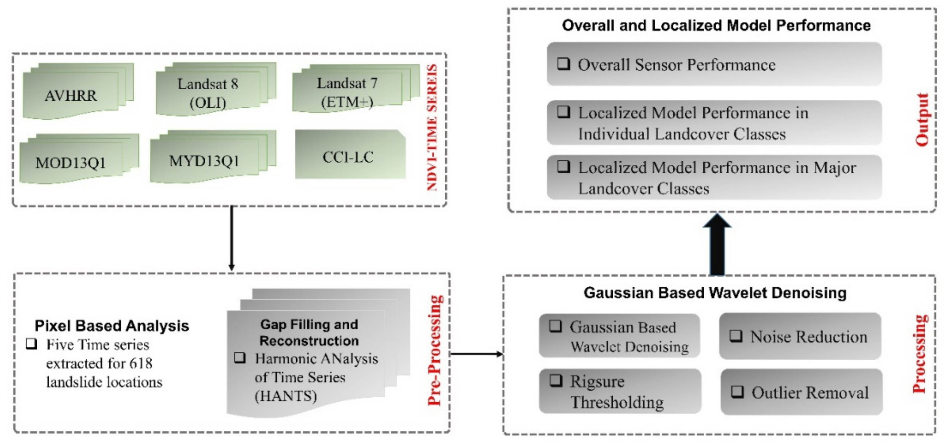
2. Materials and Methods

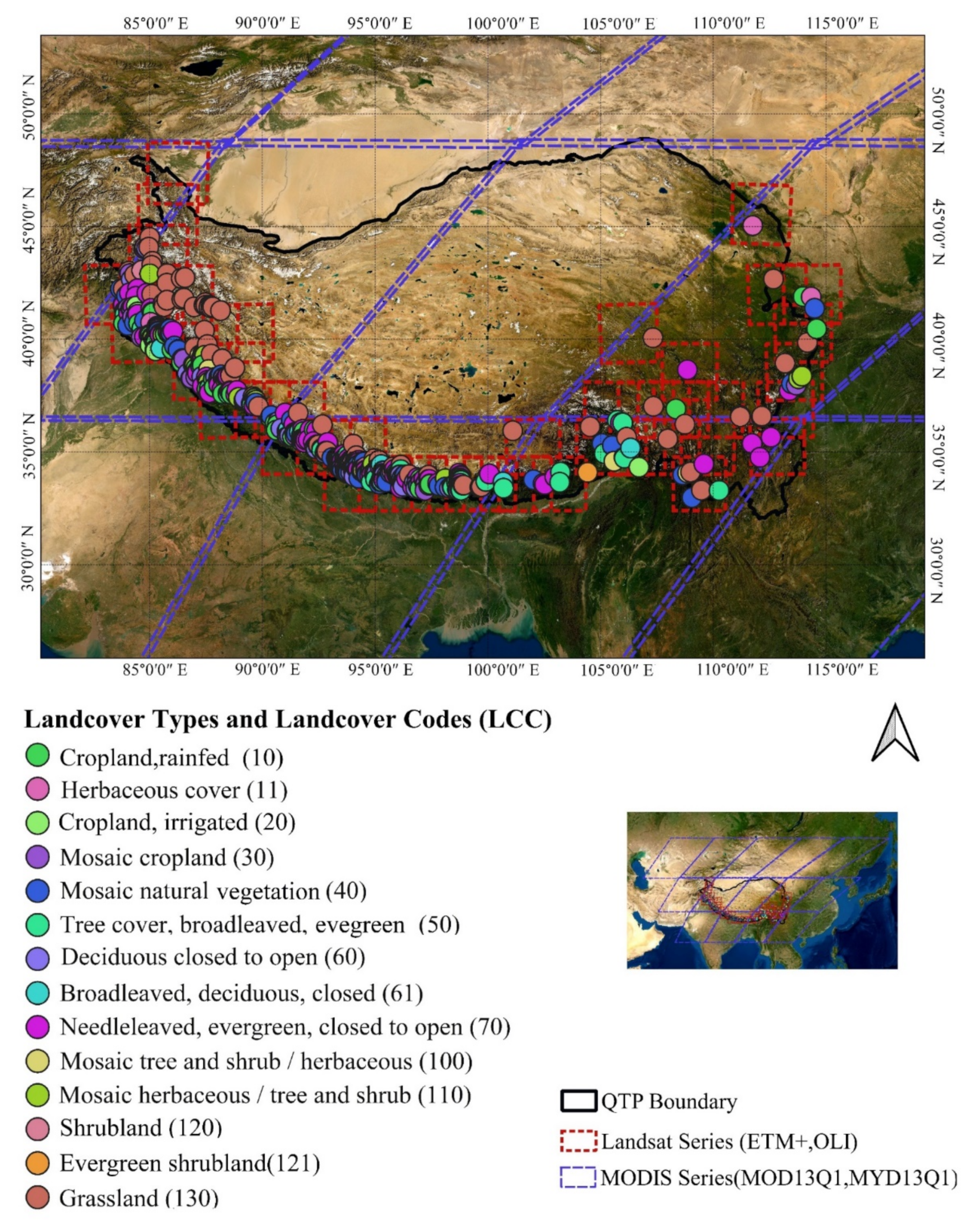
2.1. Study Area

The Qinghai-Tibetan Plateau (QTP), with a total area of about 2,572,400 km², is located in southwestern China (74°–104°E, 25°–40°N, see Figure 1) [62,63]. It is the highest (average altitude > 4000 m ASL) and largest plateau in the world with unique topography. Due to its structure complexity, the QTP is characterized by low temperatures ranging from −15 °C to 10 °C and low precipitation, with cold and arid climatic conditions in winter controlled by Siberian high and Mongolian high, and semi-arid climate in summer controlled by the South Asian monsoon system [33,64,65].

The vegetation cover in QTP mainly includes steppe, shrub, desert, meadow, forest, barren areas (bare soil), and water bodies (ice and glacier) [38,66]. The major ecoregions in QTP are composed of Karakoram–West Tibetan Plateau alpine steppe, Central Tibetan Plateau alpine steppe, Tibetan Plateau alpine shrublands and meadows, Southeast Tibet shrublands and meadows, North Tibetan Plateau–Kunlun Mountains alpine desert, and the Yarlung Tsangpo arid steppe (Olson et al. 2001). The alpine grasslands (alpine steppe and meadow) cover about 59.15% (approximately 1,521,500 km²) of the total QTP [53,67]. The Himalayan regions around the southern boundary of QTP are considered the landslide hotspots and cause hundreds to thousands of casualties each year [9,11].

This study focuses on the 618 landslide-prone locations (see Figure 1) in the Himalayan region and its surrounding areas. In southern Himalayas (landslide locations), there is a shift of vegetation cover from rainforest westward to needle leaf forest, shrub, meadow, and snow (glacier) (Peng et al., 2012). A total of fourteen major vegetation classes were identified for the 618 landslide locations. The landslide locations were obtained from the NASA Global Landslide Catalog (GLC), which contains information about landslides locations and characteristics from 2007–2016 [11]. The GLC chiefly gathers landslide information from numerous datacenters, including the International Consortium on Landslides; International Landslide Centre, University of Durham; EM-DAT International Disaster Database; International Federation of Red Cross and Red Crescent Societies field reports; Reliefweb; humanitarian disaster information run by the United Nations Office for the Coordination of Humanitarian Affairs; and other online regional and national newspaper articles and media sources. The GLC has the best resolution at 0.2° [68,69], and it has been used in different landslide studies at the global and regional scale, especially the QTP region [11,69,70,71,72].

2.2. Data Used

In this study, five NDVI source data (AVHRR, MOD, MYD, ETM+, and OLI) covering the QTP during 2000–2020 from Google Earth Engine (GEE) were collected to compare their performances. Overall, about 10,000 satellite imageries were analyzed. All products were corrected, cloud masking was considered in calculations, and cloud pixels were removed. The NDVI is used to estimate vegetation dynamics, and it is the normalized ratio of the near-infrared (NIR) to red (RED) reflectance $\left(\raisebox{1ex}{$\mathsf{\rho }\mathrm{NIR}$}\!\left/ \!\raisebox{-1ex}{$\mathsf{\rho }\mathrm{RED}$}\right.\right)$:

$$\mathrm{NDVI}=\frac{\mathsf{\rho }\mathrm{NIR}-\mathsf{\rho }\mathrm{RED}}{\mathsf{\rho }\mathrm{NIR}+\mathsf{\rho }\mathrm{RED}}$$

(1)

where ρNIR is the surface reflectance measured at the near-infrared channel and ρNIR refers to the surface reflectance measured in the red channel of satellite imagery. In general, higher NDVI values indicate healthier vegetation, whereas negative values (close to 0) indicate bare soil or snow [73,74,75]. A pixel-based approach was applied to compare the five NDVI datasets performance in the study area to extract NDVI values for the 618 landslide sites. The long NDVI data products and their specifications are tabulated in

Table 2. Remote sensing data and their specifications used for this study.

Sensors/Model	Temporal Resolution (day)	Spatial Resolution (m)	Bands	Data Source
NOAA-AVHRR-NDVI-V5	1	0.05°	NDVI	http://ltdr.nascom.nasa.gov (accessed on 10 July 2020 from GEE)
MYD13Q1	16	250	NDVI	https://lpdaac.usgs.gov/products/myd13q1v006/ (accessed on 10 July 2020 from GEE)
MOD13Q1	16	250	NDVI	https://lpdaac.usgs.gov/products/mod13q1v006/ (accessed on 10 July 2020 from GEE)
Landsat 7	16	30	NIR, R	http://landsat.usgs.gov/CDR_LSR (accessed on 10 July 2020 from GEE)
Landsat 8	16	30	NIR, R	http://landsat.usgs.gov/CDR_LSR (accessed on 10 July 2020 from GEE)

and described below.

2.2.1. NOAA-AVHRR-NDVI-V5

The NOAA Climate Data Record (CDR) of the Advanced Very High-Resolution Radiometer (AVHRR V5) sensor has a 1-day temporal resolution and 0.05° spatial resolution [76,77]. It includes the daily NDVI values obtained from NOAA-AVHRR surface reflectance data [75,78]. The AVHRR sensor is highly sensitive to water vapor in the atmosphere due to the broader bandwidths that affect pixel quality [42,44,79]. Therefore, the Quality Assurance (QA) products were used to select the least cloud-contaminated pixels in the dataset. QA layer provides useful information about each pixel overall cloud contamination and validates the value of the individual channel for each pixel [80]. In this study, based on the QA band information, low-quality pixels were removed, and high-quality pixels were considered for analysis.

2.2.2. MODIS-NDVI (MOD13Q1-MYD13Q1)

The Moderate Resolution Imaging Spectroradiometer (MODIS) vegetation index products are designed to provide a consistent spatiotemporal monitor of vegetation dynamics and have been in production continuously since 2000 [48,81,82]. This study used the MOD13Q1 and MYD13Q1 NDVI products (version 006) with 16-day and 250 m resolutions. Both products contain QA flags that hold information about pixel usefulness, which excludes bad pixels with cloud and shadows [42,83]. The usefulness index was applied so that “good” quality pixels (based on QA band) were selected, and the rest are excluded from both sensors.

2.2.3. Landsat Series (7 and 8)

Different Landsat series (4–8) have been providing information since 1972 to present at different spatial resolutions [84]. Landsat series have near-polar orbits, repeating every 16 days. Two latest sensors (ETM+, OLI) are used to derive long NDVI datasets at 30 m spatial resolution. We used USGS Landsat 7 and 8 Surface Reflectance Climate Data Records (LSR-CDR) in this study. LSR-CDR is processed and orthorectified [75,85] based on the National Aeronautics and Space Administration (NASA)-funded Landsat Ecosystem Disturbance Adaptive Processing System (LEDAPS) program. Additionally, LSR-CDR data have been atmospherically corrected using LEDAPS and include a cloud, shadow, water, and snow mask produced using CFMASK [48,51] as well as a per-pixel saturation mask [86]. The QA layer obtained from cloud masks [48,51,87] was used to select the highest quality pixels, lowest cloud, and shadow contaminations. Thus, the 16-day NDVI dataset was produced from these corrected reflectance data using Equation (1).

2.2.4. Land Cover Dataset

European Space Agency (ESA) Climate Change Initiative Land Cover (CCI-LC) provides long time series of global data designed explicitly for global landcover characterization [88] and vegetation analysis [89,90,91]. ESA CCI-LC maps were published as the first series of annual 300 m (spatial resolution) global land cover maps for 24 years, from 1992 to 2015, integrating several ground observation products based on ESA GlobCover products with 71.1% accuracy [92,93]. This study used the ESA CCI-LC data (http://maps.elie.ucl.ac.be/CCI/viewer/download.php; accessed on 18 July 2020) from 2000–2015 (38 land cover classes), and the majority of land cover types for each pixel was considered as the landcover type of the given pixel. Landcover classes were extracted for the 618 landslide locations, and those classes with low data content (Shrubland LCC 120 and evergreen shrubland LCC 121 with one observation) were excluded from the analysis. Hence, a total of twelve landcover classes were identified and retained for further analysis.

2.3. Methods

The five long-term NDVI datasets in Table 2 were preprocessed using the harmonic analysis of time series (HANTS) algorithm, specifically to fill and eliminate the gaps. They were then denoised using the wavelet threshold denoising (WTD) algorithm. Figure 2 presents the methodology adopted for the preprocessing and denoising of the five NDVI datasets.

2.3.1. Harmonic Analysis of Time Series (HANTS) Algorithm

Noise, interruption, loss (missing), or contamination within the original NDVI datasets usually occur due to cloud, atmosphere, and climatic conditions that limit NDVI applications [47,48,49,51]. Thus, it is necessary to derive an effective method (gap filling and de-noising) to extract meaningful information from the original NDVI dataset. In this study, the HANTS algorithm [51] was implemented in the five NDVI datasets to identify and eliminate any sudden drops in observation points caused by different noise sources. Since the NDVI dataset has a generally irregular time interval (due to missing values), the HANT algorithm was explicitly used to fill the dataset’s gaps and produce a regular time interval. The HANTS algorithm transforms the time series into the frequency domain. The new time series is then reconstructed using sine and cosine basic functions, allowing the analysis of the signal content (frequency) and generating smooth variable values [45,51,94]. The general equation of HANTS to reconstruct the original data is described as:

$$NDV{I}_o\left(t_i\right)=NDV{I}_H\left(t_i\right)+\epsilon \left(t_i\right)$$

(2)

$$NDV{I}_H\left(t_i\right)=a_0+{\displaystyle \sum }_{K=1}^{nf}{A}_k, \sin \left(2\pi f_k{t}_i+{\theta }_k\right)$$

(3)

where $NDV{I}_o\left(t_i\right)$ is the observed NDVI value in time $t_i$, and $NDV{I}_H\left(t_i\right)$ is the reconstructed NDVI value, with the modelling error of $\epsilon \left(t_i\right)$; $n_f$ represents the number of frequency components $f_k$, and the $A_k$ and ${\theta }_k$ are the amplitude and phase of frequency component; ${\alpha }_0$ is the average value of time series.

The HANTS modeling can be obtained by solving the above equation using the linear least square (LLS) method. Invalid NDVI values (ice and snow flags) were removed to run the HANTS algorithm, and then the HANTS was performed separately on each NDVI dataset. The HANTS algorithm parametrization directly affects its performance; for example, the number of frequency components $\left(n_f\right)$ and degree of over-determinedness (DOD) are critical in the analysis [45,51]. The $n_f$ varies from 2–5 (three, six, nine, twelve months) in different studies [51,95,96,97,98]. In this study, the first-four frequency components related to the phenological characteristics were used separately for each year. DOD presents the regression overfitting, which can be calculated as [45]:

$$\mathrm{DOD}=\mathrm{MB}-(2\ast n_f-1)$$

(4)

where MB is the minimum number of observations. After the estimation of HANTS annual coefficients (${\alpha }_0$, $A_k$, ${\theta }_k$ for twelve months), the missing NDVI values for each year were estimated.

2.3.2. Gaussian-Based Wavelet Threshold Denoising (WTD)

After performing the HANTS to derive regular time intervals of NDVI datasets, the noise in them should be removed for the time series analysis. Numerous studies have utilized WTD for denoising and smoothing of NDVI time series [99,100,101,102]. The WTD-based method is also used in this study for handling noise in NDVI datasets.

Discrete wavelet transformation (DWT) decomposes time series into a set of sub-series using basic functions known as “mother wavelet”, $\psi \left(t\right)$ from dilation (scale), and translation (position) parameters related to low and high range frequency domains [94,103,104]. Given a proper mother wavelet $\psi \left(t\right)$ and the decomposition level, NDVI data based on WT can be defined as [105,106]:

$$W_{NDVI}\left(j,k\right)={{\displaystyle \int }}_{-\infty }^{\infty }NDVI\left(t\right){\overline{\psi }}_{j,k}\left(t\right)dt,\hspace{1em}{\psi }_{j,k}\left(t\right)a_0{}^{-j/2} \mathsf{\psi }\left(a_0{}^{-j} t-k{b}_0\right)$$

(5)

in which $a_0$, $b_0$ are constants, $k$ is time position factor (translation factor), and $j$ indicates the decomposition level. $\overline{\psi }\left(u\right)$ is the complex conjugate. $W_{NDVI}\left(j,k\right)$ is discrete wavelet coefficient of NDVI under position k and level $j$, including both the approximation coefficient (A_j) and the detail coefficient (D_j) at level j. The orthogonal DWT is used commonly by assigning $a_0=2$ and $b_0=1$ [107] which consists of ${\log }_{2}n$ levels given that the analyzed series has the length of $n$ [106,108]. Completed description of DWT can be found in [105,107,109,110,111].

The DWT which meets the regularity condition can be adopted for NDVI time series reconstruction [106]:

$$NDVI\left(t\right)={{\displaystyle \sum }}_{j,k}{W}_{NDVI}{\left(j,k\right)}_{ }\overline{\psi } \left(a_0{}^{-j} t-k{b}_0\right)$$

(6)

Wavelet threshold denoising (WTD) is based on DWT results of NDVI time series and adjusts the wavelet detail coefficients:

$$W_{NDVI’}\left(j,k\right)=TR\left(W_{NDVI}\left(j,k\right), T_j\right)$$

(7)

in which $TR$ represents the thresholding rule, $T_j$ is threshold in decomposition level j, and $W_{NDVI’}\left(j,k\right)$ is the denoised value of $W_{NDVI}\left(j,k\right)$. By substituting $W_{NDVI’}\left(j,k\right)$ into Equation (6), the denoised NDVI time series can be reconstructed. Any residuals of wavelet denoising can be further used to extract information from signal content (noise and outliers) [106,112,113].

The WTD efficiency is highly sensitive to four critical factors, including wavelet basis function, decomposition level choices, threshold estimation, and coefficient thresholding, as they influence the model accuracy [111,114]. The decomposition level is a key factor in wavelet decomposition. Several studies have used different decomposition levels for DWT [115,116,117,118]. Furthermore, Sang [105] proposed an extensive practical procedure to select the suitable decomposition level. The choice of decomposition level in this study was performed based on an empirical examination due to the complex input dataset (different NDVI time series) and the implemented algorithm (twenty decomposition levels were examined in the study). The WTD on detail coefficients was implemented in two steps:

i.

Since abrupt changes caused by outliers influence the NDVI time series, it is essential to identify and eliminate these detail coefficients. The Gaussian-based thresholding method was used in this study. Hence, based on the experimental examination, the confidence interval of −σ ~ σ + μ (68.27%, $\mu$ is mean value and $\sigma$ is standard deviation) was considered as an outlier, and those detail coefficients outside the confidence interval were removed (i.e., set as 0) [119,120].

ii.

Typical wavelet thresholding method “RIGRSURE” was performed to estimate threshold T_j [121] (in Equation (7) (Figure 3). The mathematical equation of the RIGRSURE threshold [122,123,124] can be defined as:

$$T_j=S_j\sqrt{{\omega }_k}$$

(8)

where $S_j$ is the standard deviation of the wavelet coefficient at scale j; ${\omega }_k$ represents the $k$th coefficient wavelet square (coefficient at minimal risk) at scale j.

2.4. Overall and Localized Model Performance

Performance assessment is essential to evaluate the reliability and effectiveness of the modeled NDVI time series with respect to the original dataset [125,126]. Because the accurate and timely ground reference data are inaccessible for validation, the systematic evaluation of remote sensing data from ground truth data is often challenging [127]. Hence, the performance evaluation and the reliability of the five NDVI datasets can be assessed by the absolute difference between the denoised NDVI time series and the original (observed) time series [51,125,126,128]. Likewise, this difference will point out which original NDVI series are less noisy considering the proposed denoising method. We used the following four performance criteria: correlation coefficient (CC), mean absolute error (MAE), root mean square error (RMSE), and signal to noise ratio (SNR). Let us consider $NDV{I}_i^o$ and $NDV{I}_i^D$ as the observed and denoised NDVI time series, and $\overline{NDV{I}_i^o}$ and $\overline{NDV{I}_i^D}$ their mean values, with the number N of observations; the CC, MAE, RMSE, and SNR can be derived as follows:

$$\mathrm{CC}=\frac{{{\displaystyle \sum }}_{i=1}^N\left[NDV{I}_i^o-\overline{NDV{I}_i^o}\right]\left[NDV{I}_i^D-\overline{NDV{I}_i^D}\right]}{\sqrt{{{\displaystyle \sum }}_{i=1}^N{\left[NDV{I}_i^o-\overline{NDV{I}_i^o}\right]}^2\left[NDV{I}_i^D-\overline{NDV{I}_i^D}\right]}}$$

(9)

$$\mathrm{MAE}=\frac{1}{N}{\displaystyle \sum }_{i=1}^N\left|NDV{I}_i^o-NDV{I}_i^D\right|$$

(10)

$$\mathrm{RMSE}=\sqrt{\frac{1}{N}{\displaystyle \sum }_{i=1}^N{\left(NDV{I}_i^o-NDV{I}_i^D\right)}^2}$$

(11)

In this study, we computed the SNR using the following equation [129]:

$$\mathrm{SNR}=10{\log }_{10}\left(\frac{va{r}_{NDV{I}_i^o}}{va{r}_{NDV{I}_i^D}}\right)$$

(12)

where $va{r}_{NDV{I}_i^o}$ represents the variance of $NDV{I}_i^o; va{r}_{NDV{I}_i^D}$ is the variance of $NDV{I}_i^D$.

CC is the rate of collinearity between denoised and observed NDVI time series. Higher values of CC mean higher similarity between the two-time series. RMSE indicates the rate of discrepancy between the modeled and the original NDVI time series: lower values of RMSE refer to a lower rate of dissimilarity between the two time series [130]. SNR is a well-known signal processing metric that evaluates the denoised (modeled) NDVI time series quality. Higher values of SNR signify a higher quality of denoised time series [131].

The overall model performance was provided by box-plot analysis for each sensor, considering the above metrics computed in each location (618 total). The localized performance was similarly computed for the different land cover types by clustering the pixels with similar land covers.

3. Results

The gap values for each NDVI dataset were estimated and filled using the HANTS algorithm in Equation (2), with an example shown in Figure 4 (panels A–J) for point 18 having “tree cover, broadleaved and evergreen” as landcover type. After that, the DWT algorithm with different mother wavelets and different decomposition levels was examined for denoising the NDVI time series (examples reported in Figure 4), and each NDVI dataset performance was evaluated using the criteria in Equations (9) and (10).

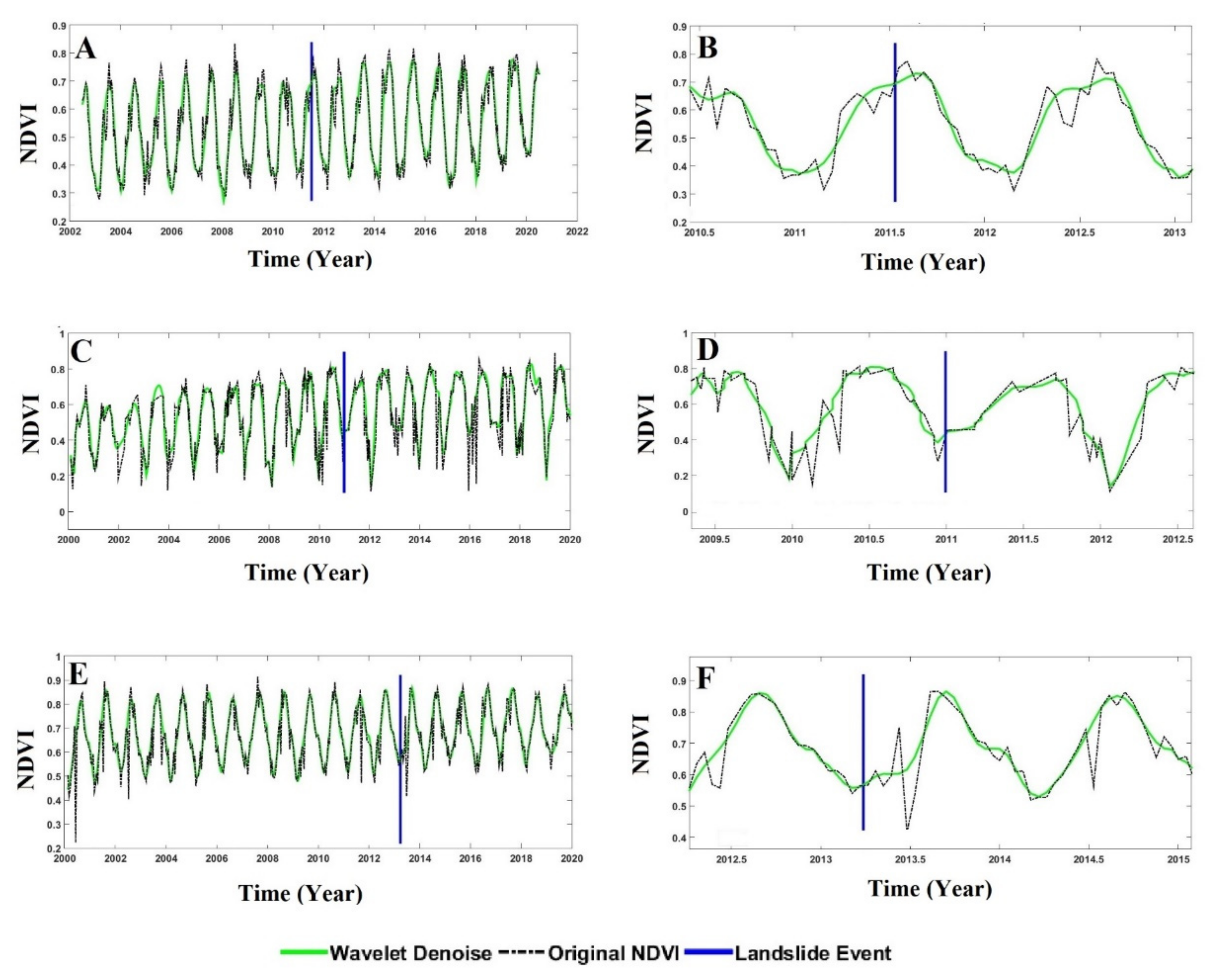
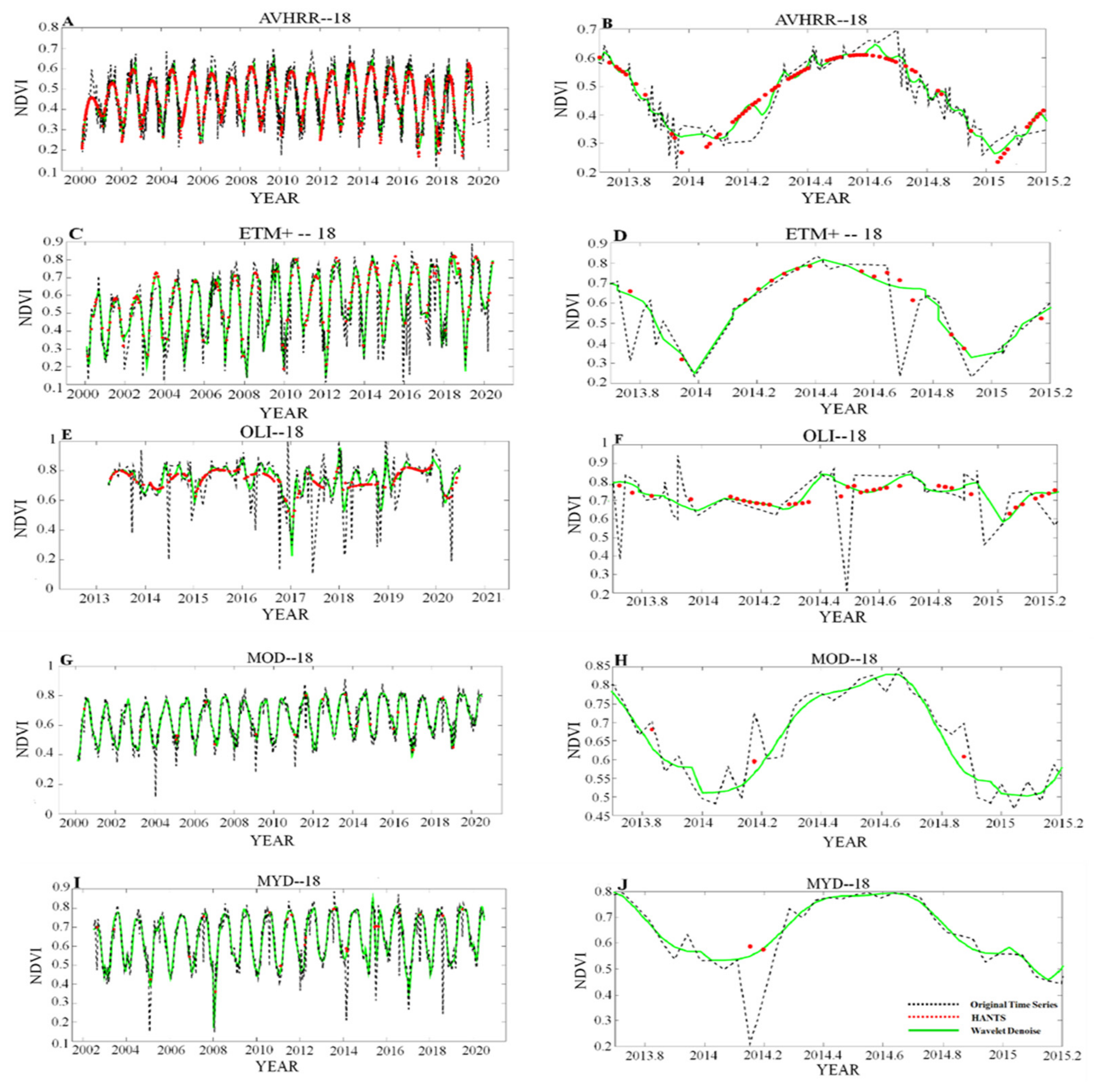
3.1. NDVI Time Series Denoising and Evaluation

To select the suitable mother wavelet, we examined different mother wavelet families, including the Daubechies (db), Symlets (sym), Coiflets (coif), BiorSplines (bior), and ReverseBior (rbio) families [132]. The AVHRR dataset was selected as the sample dataset here due to its higher temporal resolution than other datasets. The statistical analysis (boxplots) of the results obtained using different mother wavelets and different decomposition levels are shown in Figure 5 and Figure 6, respectively. They depicted that “db9” exhibited better results (RMSE = 0.096 and CC = 0.741) compared to others. In addition, the boxplot analysis reported in Figure 6 indicated that level 1 shows comparable performance to level 2, with higher levels having worse RMSE and correlation. Thus, decomposition level 2 and “db9” were selected as the most suitable mother wavelet and the best decomposition level for WTD of NDVI datasets. Daubechies family belongs to the orthogonal wavelets with the maximum number of vanishing moments, referring to mother wavelet roots and smoothness [133,134]. From Figure 5, it can be noticed that the near-symmetric “Coiflet 5” showed better performance among the Coiflet’s mother wavelets. The Coiflet wavelet has a larger number of vanishing moments in both scaling and wavelet function [135]. “Sym7” performed better among Symlet mother wavelets, which are of the modified Daubechies family with more symmetry [107]. “bior 3.5” with symmetric structure had a higher correlation among BiorSplines [136]. “rbio 2.8” showed a higher correlation than the Rbio family. Rbio is derived from biorthogonal wavelet coupled and guided by biorthogonal spline [137]. Note that more detailed information on the wavelet family refers to wavelet toolbox documentation [132].

After selecting the mother wavelet “db9” and the decomposition level 2, the Gaussian-based WTD method was implemented in the detail coefficients to identify and eliminate the high-frequency detail coefficients (out of confidence interval, 68.27%, see Section 2.3.2) caused by outliers. Therefore, each NDVI dataset of the five sensors was denoised and smoothed based on regular wavelet thresholding, as in the example previously shown in Figure 4.

As a further example, based on the NASA global landslide inventory dataset [68,70], we selected three landslide sample locations reporting the corresponding long-term original and denoised NDVI pre-and post-disaster (Figure 7A–F). Landslides can cause vegetation disturbance which affect the NDVI values, but the presence of the noise in the NDVI time series can also be misinterpreted as variations caused by the landslide events. The different noisy behaviors of the original NDVI can be recognized in the three examples reported in Figure 7.

In Figure 7A,B, the NDVI time series from MYD for the sample point located at 30.0315°N, 101.0144°E (China, large-mudslide) is reported. The landslide event occurred on 13 July 2011 at the maximum annual NDVI values. Visually, it did not cause a significant change in the annual phenological trend, and slight differences between the original and denoised NDVI were observed pre- and post-disaster. In Figure 7C,D, the NDVI from ETM+ for the sample at 29.7415°N, 81.2467°E (Nepal, medium-mudslide) is shown. The landslide event occurred on 30 December 2010 during the phenological vegetation dormancy (low NDVI), and slight differences between the denoised and original values in the annual NDVI cyclic behavior are observed. Figure 7E,F shows the NDVI from MOD at 30.0315°N, 101.0144°E (China). A very large landslide event occurred on 29 March 2013 during the phenological plant dormancy. A significant disturbance of the original NDVI was observed post-disaster, a disturbance that the smoothed denoised NDVI tried to follow. Overall, landslides may or may not cause disturbances in NDVI values. Therefore, while considering specific studies mainly based on the use of the NDVI anomalies for landslide detection, the true anomalies or the noisy values could be distinguished by considering a statistical analysis of the differences between the original and the denoised NDVI trends.

After denoising the five NDVI time series, an overall and localized (i.e., considering each vegetation class) sensor performance was carried out according to the four criteria (CC, MAE, RMSE, and SNR), and the results are presented in Figure 8 and Figure 9, and

Table 3. Statistical analysis of localized performance in five different sensors (MOD, MYD, AVHRR, ETM+, OLI) based on mean values of cross-correlation (CC), root mean square (RMSE), and signal to noise ratio (SNR) in different landcover classes over QTP *.

Landcover Codes (LCC)	LC (%)	MOD13Q1			MYD13Q1			AVHRR			ETM+			OLI
		RMSE	CC	SNR	RMSE	CC	SNR	RMSE	CC	SNR	RMSE	CC	SNR	RMSE	CC	SNR
Cropland, rainfed (10)	8.90	0.043	0.941	20.505	0.048	0.939	20.299	0.025	0.965	25.423	0.026	0.967	24.081	0.021	0.976	27.092
Herbaceous cover (11)	3.56	0.046	0.937	20.434	0.048	0.944	20.292	0.022	0.976	26.054	0.032	0.957	22.877	0.023	0.979	26.630
Cropland, irrigated (20)	3.07	0.049	0.863	18.161	0.055	0.812	17.091	0.027	0.944	24.201	0.026	0.951	22.613	0.020	0.96	25.826
Mosaic cropland (30)	7.28	0.048	0.919	20.634	0.047	0.913	20.210	0.022	0.966	26.448	0.025	0.958	23.717	0.021	0.971	27.839
Mosaic natural vegetation (40)	15.37	0.050	0.905	20.156	0.058	0.877	19.556	0.022	0.973	27.332	0.029	0.961	23.635	0.021	0.980	28.354
Tree cover, broadleaved, evergreen (50)	6.95	0.073	0.834	19.402	0.086	0.816	18.170	0.017	0.982	30.075	0.033	0.94	24.721	0.024	0.968	29.142
Deciduous closed to open (60)	8.09	0.053	0.912	20.368	0.060	0.898	19.618	0.024	0.969	26.265	0.028	0.957	23.898	0.023	0.972	27.202
Broadleaved, deciduous, closed (61)	3.56	0.055	0.903	20.448	0.065	0.877	19.061	0.020	0.973	28.246	0.030	0.953	24.626	0.020	0.974	29.102
Needle-leaved, evergreen, closed to open (70)	22.97	0.067	0.869	19.263	0.066	0.865	18.491	0.021	0.974	27.452	0.033	0.961	23.653	0.028	0.966	26.393
Mosaic tree and shrub/herbaceous (100)	1.45	0.065	0.888	19.100	0.063	0.86	19.107	0.020	0.972	28.112	0.029	0.965	25.330	0.028	0.971	25.821
Mosaic herbaceous/tree and shrub (110)	5.17	0.058	0.88	18.143	0.063	0.849	17.409	0.023	0.966	26.937	0.031	0.963	23.864	0.022	0.962	27.762
Grassland (130)	13.26	0.039	0.873	17.581	0.042	0.865	16.763	0.013	0.961	25.350	0.016	0.962	23.216	0.011	0.978	26.855
Overall Performance		0.052	0.894	19.724	0.055	0.879	18.955	0.021	0.972	26.236	0.030	0.96	23.562	0.022	0.973	27.220
Performance Range **		0.048	0.148	7.006	0.052	0.154	7.139	0.036	0.151	7.636	0.076	0.374	5.935	0.083	0.208	8.290

* The numbers in bold indicate the four main vegetation classes in QTP. ** Performance range: RMS/CC/SNR difference between maximum and minimum values.

. Each sensor was evaluated considering the behavioral similarity between the original (observed) and the denoised NDVI time series. Specifically, the ability to preserve the original shape (CC) and the time series values (MAE, RMSE, SNR) was quantified. This analysis will also determine the sensor providing the original NDVI series with less noise on the basis of the proposed denoising approach. In Table 3, the four major landcover classes are also highlighted, i.e., needle-leaved, evergreen, closed to open (LCC 70; LC% = 22.97%, where LCC and LC% are the landcover code and area percentage, respectively), mosaic natural vegetation (LCC 40; LC% = 15.37%), grassland (LCC 130; LC% =13.26%), and cropland (LCC10; LC% = 8.90%).

3.2. Results of AVHRR Dataset

The AVHRR-NDVI product inherently has a noisy data structure as a major drawback in vegetation monitoring applications [42], because it was not initially designed for this purpose [79,138]. Although the QA band eliminates most of the cloud and shadow effects in the data, there are still consecutive local fluctuations with different amplitudes. Besides, the presence of annual and inter-annual patterns revealed that the HANTS could model the overall trend, and then WTD modeled these local patterns as well as local variations (Figure 4A,B). The overall performance metrics from the median quartile $\left(\mathrm{CC}=0.972, \mathrm{MAE}=0.015, \mathrm{RMSE}=0.021, \mathrm{and} \mathrm{SNR}=26.236\right)$ were higher than MODIS and very comparable to the Landsat 8 ones (Figure 9, and Table 3). The sensor performance ranges were 0.151, 0.013, 0.036, and 7.636 for correlation coefficient, MAE, RMSE, and SNR, respectively. Additionally, the localized performance of AVHRR showed the highest performance of the sensor $\left(\mathrm{CC}=0.974, \mathrm{MAE}=0.014, \mathrm{RMSE}=0.021, \mathrm{and} \mathrm{SNR}=27.452\right)$ in first-dominant land cover in QTP (needle-leaved, evergreen, closed to open LC% = 22.97%) (Figure 9, Table 3).

3.3. Results of Landsat Dataset (ETM+, OLI)

ETM+ analysis and statistical performance (Figure 4C,D) indicated that both the HANTS and WTD algorithms underestimate the maximum annual NDVI values, which may have reduced sensor performance compared to OLI. The overall sensor performance was acceptable $\left(\mathrm{CC}=0.960, \mathrm{MAE}=0.022, \mathrm{RMSE}=0.030, \mathrm{and} \mathrm{SNR}=23.562\right)$ as it showed better performance in most land cover classes than the MODIS series (Figure 8, Table 3). The maximum performance of the sensor (highest correlation coefficient and SNR, with minimum MAE, RMSE) occurred with values 0.967, 24.081, 0.019, and 0.016, respectively, in cropland and grassland classes (Figure 9, Table 3). The sensor performance ranges were 0.374, 0.018, 0.076, and 5.935 for CC, MAE, RMSE, and SNR, respectively.

OLI showed that the annual sensor behavior was relatively smooth, as the HANTS and WTD algorithms modeled the NDVI time series with a minimum degree of fluctuation (smooth local maximum) (Figure 4E,F). The results also referred to the minimum modeling deviation from the original shape of the data, which leads to higher overall $\left(\mathrm{CC}=0.973, \mathrm{MAE}=0.015, \mathrm{RMSE} =0.022, \mathrm{and} \mathrm{SNR}=27.220\right)$ and localized performance in different classes $\left(\mathrm{CC}>0.960, \mathrm{MAE}\le 0.021, \mathrm{RMSE}\le 0.028, \mathrm{and} \mathrm{SNR}>25.821\right)$ (Figure 8 and Figure 9, and Table 3). The sensor performance ranges were 0.208, 0.025, 0.0017, 0.083, and 8.290 for CC, MAE, MSE, RMSE, and SNR, respectively. Finally, OLI showed the highest localized performance in the second, third, and fourth dominant land cover classes in QTP (mosaic natural vegetation LC% = 15.37%, grassland LC% = 13.26%, and cropland LC% = 8.90%) (Table 3).

3.4. Results of MODIS Dataset (AQUA, TERRA)

Figure 4G–J shows that the HANTS algorithm slightly underestimates the annual behavior of MODIS-NDVI (MOD, MYD), as it fails to model the maximum annual NDVI values, while the use of the WTD algorithm modeled this underestimation well. As shown in Figure 4G,J, WTD smoothly modeled NDVI and ignored sudden disturbances. The results also indicated a slight deviation of modeling from the original shape of the data with overall acceptable performance for MOD $\left(\mathrm{CC}=0.894, \mathrm{MAE}=0.039, \mathrm{RMSE}=0.051, \mathrm{and} \mathrm{SNR}=19.724\right)$ and MYD $\left(\mathrm{CC}=0.879, \mathrm{MAE}=0.041, \mathrm{RMSE}=0.055, \mathrm{SNR}=18.955\right)$ (Figure 8, Table 3). The sensors performance ranges were 0.148, 0.034, 0.006, and 7.006 $\left(\mathrm{CC}, \mathrm{MAE}, \mathrm{RMSE}, \mathrm{and} \mathrm{SNR}\right)$ for MODIS TERAA, and 0.154, 0.038, 0.052, and 7.139 $\left(\mathrm{CC}, \mathrm{MAE}, \mathrm{RMSE}, \mathrm{and} \mathrm{SNR}\right)$ for MYD. This indicates that both sensors are statistically consistent and have a similar range of variability. However, the MOD sensor with lower RMSE and higher correlation showed relatively better performance than MYD. The lowest MAE, RMSE, and the highest correlation (CC) and SNR belonged to grassland and cropland $\left(\mathrm{MAE}=0.032, \mathrm{RMSE}=0.039, \mathrm{CC}=0.941, \mathrm{and} \mathrm{SNR}=20.505\right)$ for the MOD (Figure 9, Table 3) and the grassland and herbaceous cover for the MYD $\left(\mathrm{MAE}=0.034, \mathrm{RMSE}=0.042, \mathrm{CC}=0.944, \mathrm{and} \mathrm{SNR}=20.292\right)$ (Figure 9, Table 3).

Overall, OLI relatively outperformed the other sensors based on the four metrics: i.e., the original OLI NDVI is less noisy with respect to the original NDVI from the other sensors. It showed the highest localized performance in the second, third, and fourth dominant land cover classes, specifically, mosaic natural vegetation $\left(\mathrm{LC}\%=15.37\%, \mathrm{CC}=0.980, \mathrm{MAE}=0.014, \mathrm{RMSE} =0.021,\mathrm{and} \mathrm{SNR}=28.354\right)$, grassland $\left(\mathrm{LC}\%=13.26\%, \mathrm{CC}=0.978, \mathrm{MAE}=0.015, \mathrm{RMSE} =0.011, \mathrm{and} \mathrm{SNR}=26.855\right)$, and cropland, rainfed $\left(\mathrm{LC}\%=8.90\%, \mathrm{CC}=0.976, \mathrm{MAE}=0.015, \mathrm{RMSE} =0.021, \mathrm{and} \mathrm{SNR}=27.092\right)$. AVHRR showed an overall performance comparable to OLI with subtle differences in the major vegetation classes, while MODIS series (MOD, MYD) showed a lower overall performance.

4. Discussion

Landslide events may occur at a different time of the vegetation phenology and can be detected through an NDVI anomaly and change detection techniques between pre- and post-landside disasters [139,140]. Previous studies have shown that the vegetation disturbance due to the landslide events has a significant impact on NDVI values in the landslide locations [139,141,142]. The presence of the noise in the NDVI time series might be misinterpreted as the anomaly caused by landslide events in NDVI. This anomaly should be statistically clarified by considering the difference between the original and the denoised NDVI time series to identify NDVI anomalies related to landslide events. Furthermore, smooth annual cyclic behaviors of NDVI time series are often influenced by environmental factors that cause defects in its intrinsic behavior, which can be addressed through mathematical and statistical modeling. Among the various methods proposed for NDVI time series analysis, the HANTS (sine and cosine basis functions) is a robust method for reconstructing the NDVI time series and estimating missing values [51,143,144,145]. Besides, WTD has been proven to be a compelling method for time series analysis of such non-stationary data with different basic functions [111]. Due to the importance of NDVI in different applications and the existence of different datasets for monitoring NDVI and specific attributes of the study area (QTP) in terms of natural hazards (floods, landslides, etc.), reconstruction, modeling, and comparison of the five NDVI datasets were successfully implemented in different land cover classes in this study.

Although the AVHRR has a higher temporal resolution, its inherent characteristics, such as design, significant water vapor absorption due to broader bandwidth than the other sensors, and low spatial resolution, have led to exhibit noisy behavior in the dataset, especially in the QTP region [42,44,61,73,78,146,147]. To overcome this, the use of cloud filters and shadow masks in the QA band can eliminate large numbers of poor-quality pixels and improve the annual cycle behavior of the NDVI time series [148]. However, the QA-band-filtered data still contained noise in sequential fluctuations, identified and modeled in a satisfactory way by using HANTS and WTD (Figure 4A,B). The sensor showed the best performance in the first dominant vegetation class (needle-leaved, evergreen, closed to open; LC = 22.97%) in the QTP. MODIS (MOD, MYD) is commonly used as reference data for long NDVI time series analysis [42], and both MOD and MYD use a similar NDVI compositing algorithm [83,149]. The main difference between the two sensors is their equator crossing time (10:35 am for MOD, 1:35 pm for MYD) [148]. Their localized performance and the range of variability $\left(\mathrm{MOD}:\mathrm{CC}=0.148, \mathrm{MAE}=0.034, \mathrm{RMSE}=0.048,\mathrm{SNR}=7.006, \mathrm{and} \mathrm{MYD}:\mathrm{CC}=0.154, \mathrm{MAE}=0.038, \mathrm{RMSE}=0.052 , \mathrm{SNR}=7.139\right)$ were almost the same, with slightly better performance of the MOD sensor in most classes, consistent with previous findings [148]. The maximum difference between these two sensors was observed in tree cover, broadleaved, evergreen, and the least difference in mosaic cropland. However, the results showed a relatively higher MAE, RMSE, with lower CC, and SNR values for MODIS compared to the other sensors, which might be related to the higher number of artifacts (abrupt shifts) observed in the original data, that HANTS and WTD handle quite well.

The OLI-NDVI time series were characterized by gaps and cloud contamination (about 35% of imageries) [150,151], which ultimately performed better than the MODIS (MOD, MYD) and AVHRR datasets. Although the cloud masking algorithm (CFMASK) [48,51] created gaps in the dataset, the HANTS and WTD algorithms were able to preserve the original behavior and model the NDVI time series well (see Figure 8 and Figure 9). The overall and localized performance of OLI and AVHRR were higher than the other sensors in all vegetation classes, which indicates the consistency of the NDVI time series, especially in the OLI dataset. As mentioned above, the better performance of the OLI sensor indicates that the original NDVI time series obtained from Landsat 8 can show the interannual and cyclic behavior of the NDVI dataset with a lower amplitude of the noisy fluctuations compared to the other sensors.

Additionally, the overall performance variability in OLI showed a significant agreement with ETM+ with 0.013, 0.007, 0.008, and 3.658 differences in CC, MAE, RMSE, and SNR values, which is consistent with previous studies and shows that two sensors can be used as complementary data [152]. However, as the newest satellite in the Landsat series, OLI performs better than ETM+ due to the main differences in characteristics such as time span, spectral bandwidth (narrower), radiometric resolution, calibration, signal-to-noise ratio [35,47,48,152,153,154].

In summary, the result shows that the original NDVI datasets are inherently noisy with missing values and outliers. To reduce the inconsistencies of these native NDVI datasets, reconstruction (gap-filling), smoothing, and modeling of the NDVI time series are required in the vegetation studies. The integration of HANTS for reconstruction and WTD for denoising and modeling NDVI datasets is critical for monitoring long-term vegetation dynamics, especially in mountainous zones and landslide-prone areas with sparse vegetation covers. Although different NDVI time series have different spatiotemporal resolutions, in this study, our primary focus was on reconstructing (gap-filling) and denoising the NDVI time series based on the temporal resolution. The pixel-based performance behavior between the denoised and the original NDVI time series was evaluated for each sensor separately, but no intercomparison was done between different NDVI values among different sensors. Hence, the spectral and spatial resolution difference between different sensors has not been considered as a constraint for this study. In this context, the better performance in the temporal modeling of the OLI sensor and its better spatial resolution indicate that this sensor is the best option for vegetation monitoring in the QTP area.

The main limitation of the implemented algorithms is the high sensitivity to the types of landcovers. For example, bare soils with very low NDVI content cannot reflect the behavior of harmonic-cyclic annual and inter-annual NDVI datasets. Therefore, HANTS and WTD may not be able to reconstruct and model time series of such land cover successfully.

5. Conclusions

Vegetation as a major dynamic conditioning factor plays an important role in landslide detection by investigating the temporal variation in vegetation using NDVI time series. The existence of several NDVI products often makes it challenging to identify the ideal sensor for vegetation monitoring related to landslide studies. Identifying the best-performing sensor is essential for vegetation monitoring, and provides a unique baseline for future landslide studies, especially landslide modeling (spatial and temporal) in the region, which requires accurate information from various landslide conditioning factors (LCFs), including the NDVI as a prominent dynamic factor.

In such cases, application of advanced noise removal techniques, and comparisons between different NDVI datasets, are essential to ascertain the best sensor performance for spatiotemporal NDVI analysis. Hence, a pixel-based analysis of NDVI time series at landslide-prone locations, detecting and modelling the residual effect of noise on atmospherically and environmentally corrected data, was designed in this study to compare the performance of five popular (ETM+, OLI, MOD, MYD, and AVHRR sensors) long-term NDVI datasets. We used the HANTS and WTD algorithms to reconstruct and denoise the five NDVI datasets over 20 years at 618 landslide-prone locations in QTP. The performance assessment was based on the behavioral similarity between the original (observed) and denoised NDVI time series, considering the preservation of the original shape $\left(\mathrm{CC}\right)$ and time series values (MAE, RMSE, SNR).

The analysis showed that OLI outperformed the other sensors: that is, the native OLI NDVI series are less noisy considering the proposed denoising method. Although statistical and behavioral similarities were found between the Landsat series, MODIS series, and AVHRR-Landsat series, OLI showed the highest localized results in the second, third, and fourth dominant land cover classes in QTP.

OLI showed a better performance in the temporal modeling (gap-filling and denoising), and hence, it can be considered as a better option for long-term NDVI analysis in the QTP region. However, further investigation is recommended to assess the sensor capability for modeling the NDVI behavior in different vegetation classes in other areas. In addition, since the AVHRR NDVI dataset has shown results comparable to OLI and it has a higher temporal resolution, downscaling the AVHRR dataset into finer spatial resolutions can be a viable alternative for NDVI analysis in QTP. By fusing the AVHRR and OLI data, more reliable results of landslide studies in QTP could be obtained in the future. Overall, this study showed that the native NDVI dataset is inherently noisy, with missing values and outliers. The implementation of HANTS for gap-filling and WTD for denoising is fundamental for handling reliable and complete long-term NDVI time series, especially in landslide prone areas. Due to its effectiveness for reconstruction and denoising different NDVI time series, HANTS and WTD can be used in more recent NDVI time series such as Sentinel series, or even Landsat 9 in future, with an increase in the time span, larger number of samples, and a larger number of land cover classes for trend analysis, vegetation monitoring, and change detection at global and regional scales.

References

1. Chang, D. The vegetation zonation of the Tibetan Plateau. Mt. Res. Dev. 1981, 1, 29–48. [Google Scholar] [CrossRef]
2. Hua, W.; Fan, G.; Zhou, D.; Ni, C.; Li, X.; Wang, Y.; Liu, Y.; Huang, X. Preliminary analysis on the relationships between Tibetan Plateau NDVI change and its surface heat source and precipitation of China. Sci. China Ser. D Earth Sci. 2008, 51, 677–685. [Google Scholar] [CrossRef]
3. Fassnacht, F.E.; Schiller, C.; Kattenborn, T.; Zhao, X.; Qu, J. A Landsat-based vegetation trend product of the Tibetan Plateau for the time-period 1990–2018. Sci. Data 2019, 6, 78. [Google Scholar] [CrossRef]
4. Tian, L.; Chen, J.; Zhang, Y. Growing season carries stronger contributions to albedo dynamics on the Tibetan plateau. PLoS ONE 2017, 12, e0180559. [Google Scholar] [CrossRef] [PubMed] [Green Version]
5. Deng, H.; Wu, L.Z.; Huang, R.Q.; Guo, X.G.; He, Q. Formation of the Siwanli ancient landslide in the Dadu River, China. Landslides 2017, 14, 385–394. [Google Scholar] [CrossRef]
6. Qi, T.; Meng, X.; Qing, F.; Zhao, Y.; Shi, W.; Chen, G.; Zhang, Y.; Li, Y.; Yue, D.; Su, X.; et al. Distribution and characteristics of large landslides in a fault zone: A case study of the NE Qinghai-Tibet Plateau. Geomorphology 2021, 379, 107592. [Google Scholar] [CrossRef]
7. Yao, T.; Xue, Y.; Chen, D.; Chen, F.; Thompson, L.; Cui, P.; Koike, T.; Lau, W.K.M.; Lettenmaier, D.; Mosbrugger, V.; et al. Recent third pole’s rapid warming accompanies cryospheric melt and water cycle intensification and interactions between monsoon and environment: Multidisciplinary approach with observations, modeling, and analysis. Bull. Am. Meteorol. Soc. 2019, 100, 423–444. [Google Scholar] [CrossRef]
8. Zhao, B.; Zhao, X.; Zeng, L.; Wang, S.; Du, Y. The mechanisms of complex morphological features of a prehistorical landslide on the eastern margin of the Qinghai-Tibetan Plateau. Bull. Eng. Geol. Environ. 2021, 80, 3423–3437. [Google Scholar] [CrossRef]
9. Nadim, F.; Kjekstad, O.; Peduzzi, P.; Herold, C.; Jaedicke, C. Global landslide and avalanche hotspots. Landslides 2006, 3, 159–173. [Google Scholar] [CrossRef]
10. Petley, D. Global patterns of loss of life from landslides. Geology 2012, 40, 927–930. [Google Scholar] [CrossRef]
11. Stanley, T.; Kirschbaum, D.B.; Pascale, S.; Kapnick, S. Extreme precipitation in the Himalayan landslide hotspot. Adv. Glob. Chang. Res. 2020, 69, 1087–1111. [Google Scholar] [CrossRef]
12. Pourghasemi, H.R.; Kornejady, A.; Kerle, N.; Shabani, F. Investigating the effects of different landslide positioning techniques, landslide partitioning approaches, and presence-absence balances on landslide susceptibility mapping. Catena 2020, 187, 104364. [Google Scholar] [CrossRef]
13. Ahmad, H.; Ningsheng, C.; Rahman, M.; Islam, M.M.; Pourghasemi, H.R.; Hussain, S.F.; Habumugisha, J.M.; Liu, E.; Zheng, H.; Ni, H.; et al. Geohazards susceptibility assessment along the upper indus basin using four machine learning and statistical models. ISPRS Int. J. Geo. Inf. 2021, 10, 315. [Google Scholar] [CrossRef]
14. Saha, S.; Arabameri, A.; Saha, A.; Blaschke, T.; Ngo, P.T.T.; Nhu, V.H.; Band, S.S. Prediction of landslide susceptibility in Rudraprayag, India using novel ensemble of conditional probability and boosted regression tree-based on cross-validation method. Sci. Total Environ. 2021, 764, 142928. [Google Scholar] [CrossRef]
15. Adnan, M.S.G.; Rahman, M.S.; Ahmed, N.; Ahmed, B.; Rabbi, M.F.; Rahman, R.M. Improving spatial agreement in machine learning-based landslide susceptibility mapping. Remote Sens. 2020, 12, 3347. [Google Scholar] [CrossRef]
16. Choi, J.; Oh, H.J.; Lee, H.J.; Lee, C.; Lee, S. Combining landslide susceptibility maps obtained from frequency ratio, logistic regression, and artificial neural network models using ASTER images and GIS. Eng. Geol. 2012, 124, 12–23. [Google Scholar] [CrossRef]
17. Ozturk, U.; Pittore, M.; Behling, R.; Roessner, S.; Andreani, L.; Korup, O. How robust are landslide susceptibility estimates? Landslides 2020, 18, 681–695. [Google Scholar] [CrossRef]
18. Moreiras, S.M. Climatic effect of ENSO associated with landslide occurrence in the Central Andes, Mendoza province, Argentina. Landslides 2005, 2, 53–59. [Google Scholar] [CrossRef]
19. Petley, D.; Hearn, G.; Hart, A.; Rosser, N.; Dunning, S.; Oven, K.; Mitchell, W. Trends in landslide occurrence in Nepal. Nat. Hazards 2007, 43, 23–44. [Google Scholar] [CrossRef]
20. Bennett, G.L.; Miller, S.R.; Roering, J.J.; Schmidt, D.A. Landslides, threshold slopes, and the survival of relict terrain in the wake of the Mendocino Triple Junction. Geology 2016, 44, 363–366. [Google Scholar] [CrossRef] [Green Version]
21. Froude, M.J.; Petley, D.N. Global fatal landslide occurrence from 2004 to 2016. Nat. Hazards Earth Syst. Sci. 2018, 18, 2161–2181. [Google Scholar] [CrossRef] [Green Version]
22. Zhao, C.; Lu, Z. Remote sensing of landslides—A review. Remote Sens. 2018, 10, 279. [Google Scholar] [CrossRef] [Green Version]
23. Mattia, C.; Bischetti, G.B.; Gentile, F. Biotechnical characteristics of root systems of typical Mediterranean species. Plant Soil 2005, 278, 23–32. [Google Scholar] [CrossRef]
24. Hu, X.-S.; Brierley, G.; Zhu, H.-L.; Li, G.-R.; Fu, J.-T.; Mao, X.-Q.; Yu, Q.-Q.; Qiao, N. An exploratory analysis of vegetation strategies to reduce shallow landslide activity on loess hillslopes, Northeast Qinghai-Tibet Plateau, China. J. Mt. Sci. 2013, 10, 668–686. [Google Scholar] [CrossRef] [Green Version]
25. Li, H.; Li, Y.; Gao, Y.; Zou, C.; Yan, S.; Gao, J. Human impact on vegetation dynamics around Lhasa, southern Tibetan Plateau, China. Sustainability 2016, 8, 1146. [Google Scholar] [CrossRef] [Green Version]
26. Kuang, Q.; Yuan, Q.Z.; Han, J.C. A remote sensing monitoring method for alpine grasslands desertification in the eastern Qinghai-Tibetan plateau. J. Mt. Sci. 2020, 17. [Google Scholar] [CrossRef]
27. Pang, G.; Wang, X.; Yang, M. Using the NDVI to identify variations in, and responses of, vegetation to climate change on the Tibetan Plateau from 1982 to 2012. Quat. Int. 2017, 444, 87–96. [Google Scholar] [CrossRef]
28. Sun, J.; Cheng, G.; Li, W.; Sha, Y.; Yang, Y. On the variation of NDVI with the principal climatic elements in the Tibetan plateau. Remote Sens. 2013, 5, 1894–1911. [Google Scholar] [CrossRef] [Green Version]
29. Zheng, Z.; Zhu, W. Uncertainty of remote sensing data in monitoring vegetation phenology: A comparison of MODIS C5 and C6 vegetation index products on the Tibetan plateau. Remote Sens. 2017, 9, 1288. [Google Scholar] [CrossRef] [Green Version]
30. Zhou, L.; Tucker, C.J.; Kaufmann, R.K.; Slayback, D.; Shabanov, N.V.; Myneni, R.B. Variations in northern vegetation activity inferred from satellite data of vegetation index during 1981 to 1999. J. Geophys. Res. Atmos. 2001, 106, 20069–20083. [Google Scholar] [CrossRef]
31. Huang, K.; Zhang, Y.; Tagesson, T.; Brandt, M.; Wang, L.; Chen, N.; Zu, J.; Jin, H.; Cai, Z.; Tong, X. The confounding effect of snow cover on assessing spring phenology from space: A new look at trends on the Tibetan Plateau. Sci. Total Environ. 2020, 756, 144011. [Google Scholar] [CrossRef]
32. Yin, H.; Cao, C.; Xu, M.; Chen, W.; Ni, X.; Chen, X. Long-term snow disasters during 1982–2012 in the Tibetan Plateau using satellite data. Geomat. Nat. Hazards Risk 2017, 8, 466–477. [Google Scholar] [CrossRef] [Green Version]
33. Zhao, H.; Liu, S.; Dong, S.; Su, X.; Wang, X.; Wu, X.; Wu, L.; Zhang, X. Analysis of vegetation change associated with human disturbance using MODIS data on the rangelands of the Qinghai-Tibet Plateau. Rangel. J. 2015, 37, 77–87. [Google Scholar] [CrossRef]
34. Tucker, C.J. Red and photographic infrared linear combinations for monitoring vegetation. Remote Sens. Environ. 1979, 8, 127–150. [Google Scholar] [CrossRef] [Green Version]
35. Zhang, Y.; Song, C.; Band, L.E.; Sun, G.; Li, J. Reanalysis of global terrestrial vegetation trends from MODIS products: Browning or greening? Remote Sens. Environ. 2017, 191, 145–154. [Google Scholar] [CrossRef] [Green Version]
36. Gholamnia, M.; Khandan, R.; Bonafoni, S.; Sadeghi, A. Spatiotemporal analysis of MODIS NDVI in the semi-arid region of Kurdistan (Iran). Remote Sens. 2019, 11, 1723. [Google Scholar] [CrossRef] [Green Version]
37. Huete, A.R.; Liu, H.Q.; Batchily, K.V.; Van Leeuwen, W. A comparison of vegetation indices over a global set of TM images for EOS-MODIS. Remote Sens. Environ. 1997, 59, 440–451. [Google Scholar] [CrossRef]
38. Peng, J.; Liu, Z.; Liu, Y.; Wu, J.; Han, Y. Trend analysis of vegetation dynamics in Qinghai-Tibet Plateau using Hurst Exponent. Ecol. Indic. 2012, 14, 28–39. [Google Scholar] [CrossRef]
39. Cihlar, J.; Ly, H.; Li, Z.; Chen, J.; Pokrant, H.; Huang, F. Multitemporal, multichannel AVHRR data sets for land biosphere studies—Artifacts and corrections. Remote Sens. Environ. 1997, 60, 35–57. [Google Scholar] [CrossRef]
40. Hall-Beyer, M. Comparison of single-year and multiyear NDVI time series principal components in cold temperate biomes. IEEE Trans. Geosci. Remote Sens. 2003, 41, 2568–2574. [Google Scholar] [CrossRef] [Green Version]
41. Li, Z.; Yan, F.; Fan, X. The Variability of NDVI over northwest China and its relation to temperature and precipitation. Int. Geosci. Remote Sens. Symp. 2003, 4, 2275–2277. [Google Scholar] [CrossRef]
42. Fensholt, R.; Rasmussen, K.; Nielsen, T.T.; Mbow, C. Evaluation of earth observation based long term vegetation trends—Intercomparing NDVI time series trend analysis consistency of Sahel from AVHRR GIMMS, Terra MODIS and SPOT VGT data. Remote Sens. Environ. 2009, 113, 1886–1898. [Google Scholar] [CrossRef]
43. Zhang, L.; Guo, H.; Ji, L.; Lei, L.; Wang, C.; Yan, D.; Li, B.; Li, J. Vegetation greenness trend (2000 to 2009) and the climate controls in the Qinghai-Tibetan Plateau. J. Appl. Remote Sens. 2013, 7, 073572. [Google Scholar] [CrossRef]
44. Yu, Z.; Wang, J.; Sun, P.; Liu, S.; Liu, W. Inconsistent NDVI trends from AVHRR, MODIS, and SPOT sensors in the Tibetan Plateau. In Proceedings of the 2013 2nd International Conference on Agro-Geoinformatics, Fairfax, VA, USA, 12–16 August 2013; pp. 97–101. [Google Scholar] [CrossRef]
45. Wen, J.; Su, Z.; Ma, Y. Reconstruction of a cloud-free vegetation index time series for the Tibetan Plateau. Mt. Res. Dev. 2004, 24, 348–353. [Google Scholar]
46. Detsch, F.; Otte, I.; Appelhans, T.; Nauss, T. A comparative study of cross-product NDVI dynamics in the Kilimanjaro region—A matter of sensor, degradation calibration, and significance. Remote Sens. 2016, 8, 159. [Google Scholar] [CrossRef] [Green Version]
47. Reed, B.C.; Brown, J.F.; VanderZee, D.; Loveland, T.R.; Merchant, J.W.; Ohlen, D.O. Measuring phenological variability from satellite imagery. J. Veg. Sci. 1994, 5, 703–714. [Google Scholar] [CrossRef]
48. Roy, D.P.; Kovalskyy, V.; Zhang, H.K.; Vermote, E.F.; Yan, L.; Kumar, S.S.; Egorov, A. Characterization of Landsat-7 to Landsat-8 reflective wavelength and normalized difference vegetation index continuity. Remote Sens. Environ. 2016, 185, 57–70. [Google Scholar] [CrossRef] [PubMed] [Green Version]
49. Van Dijk, A.; Callis, S.L.; Sakamoto, C.M.; Decker, W.L. Smoothing vegetation index profiles: An alternative method for reducing radiometric disturbance in Noaa/Avhrr data. Photogramm. Eng. Remote Sens. 1987, 53, 1059–1067. [Google Scholar]
50. Zhang, J.; Yao, F.; Zheng, L.; Yang, L. Evaluation of grassland dynamics in the northern-Tibet plateau of China using remote sensing and climate data. Sensors 2007, 7, 3312–3328. [Google Scholar] [CrossRef] [Green Version]
51. Zhou, J.; Jia, L.; Menenti, M. Reconstruction of global MODIS NDVI time series: Performance of Harmonic Analysis of Time Series (HANTS). Remote Sens. Environ. 2015, 163, 217–228. [Google Scholar] [CrossRef]
52. Piao, Y.; Yan, B.; Guo, S.; Guan, Y.; Li, J.; Cai, D. Change detection of MODIS time series using a wavelet transform. In Proceedings of the 2012 International Conference on Systems and Informatics (ICSAI2012), Yantai, China, 19–20 May 2012; pp. 2093–2097. [Google Scholar] [CrossRef]
53. Ding, M.; Li, L.; Zhang, Y.; Sun, X.; Liu, L.; Gao, J.; Wang, Z.; Li, Y. Start of vegetation growing season on the Tibetan Plateau inferred from multiple methods based on GIMMS and SPOT NDVI data. J. Geogr. Sci. 2015, 25, 131–148. [Google Scholar] [CrossRef]
54. Gao, Q.; Wan, Y.; Li, Y.; Guo, Y.; Ganjurjav; Qin, X.; Jiangcun, W.; Wang, B. Effects of topography and human activity on the net primary productivity (NPP) of alpine grassland in northern Tibet from 1981 to 2004. Int. J. Remote Sens. 2013, 34, 2057–2069. [Google Scholar] [CrossRef]
55. Yang Yuan-He, P.S.-L. Variations in grassland vegetation cover in relation to climatic factors on the Tibetan plateau. Chin. J. Plant. Ecol. 2006, 30, 1–8. [Google Scholar] [CrossRef]
56. Li, H.; Li, Y.; Shen, W.; Li, Y.; Lin, J.; Lu, X.; Xu, X.; Jiang, J. Elevation-dependent vegetation greening of the Yarlung Zangbo River basin in the Southern Tibetan Plateau, 1999–2013. Remote Sens. 2015, 7, 16672–16687. [Google Scholar] [CrossRef] [Green Version]
57. Huang, N.; He, J.S.; Niu, Z. Estimating the spatial pattern of soil respiration in Tibetan alpine grasslands using Landsat TM images and MODIS data. Ecol. Indic. 2013, 26, 117–125. [Google Scholar] [CrossRef]
58. Lu, Y.; Yan, Y.; Tao, H. Classification of vegetation in North Tibet Plateau based on MODIS time-series data. Wuhan Univ. J. Nat. Sci. 2008, 13, 273–278. [Google Scholar] [CrossRef]
59. Chu, D.; Lu, L.; Zhang, T. Sensitivity of normalized difference vegetation index (NDVI) to seasonal and interannual climate conditions in the Lhasa area, Tibetan Plateau, China. Arct. Antarct. Alp. Res. 2007, 39, 635–641. [Google Scholar] [CrossRef]
60. Piao, S.; Fang, J.; He, J. Variations in vegetation net primary production in the Qinghai-Xizang Plateau, China, from 1982 to 1999. Clim. Chang. 2006, 74, 253–267. [Google Scholar] [CrossRef]
61. Zhang, G.; Zhang, Y.; Dong, J.; Xiao, X. Green-up dates in the Tibetan Plateau have continuously advanced from 1982 to 2011. Proc. Natl. Acad. Sci. USA 2013, 110, 4309–4314. [Google Scholar] [CrossRef] [Green Version]
62. Yi-li, Z.; Du, Z.; Bing-yuan, L.I. A discussion on the boundary and area of the Tibetan Plateau in China. Geogr. Res. 2002, 21, 1–8. [Google Scholar]
63. Cui, X.; Graf, H.-F. Recent land cover changes on the Tibetan Plateau: A review. Clim. Chang. 2009, 94, 47–61. [Google Scholar] [CrossRef] [Green Version]
64. You, Q.; Fraedrich, K.; Ren, G.; Pepin, N.; Kang, S. Variability of temperature in the Tibetan Plateau based on homogenized surface stations and reanalysis data. Int. J. Climatol. 2013, 33, 1337–1347. [Google Scholar] [CrossRef] [Green Version]
65. Du, M.; Kawashima, S.; Yonemura, S.; Zhang, X.; Chen, S. Mutual influence between human activities and climate change in the Tibetan Plateau during recent years. Glob. Planet. Chang. 2004, 41, 241–249. [Google Scholar] [CrossRef]
66. Gillespie, T.W.; Madson, A.; Cusack, C.F.; Xue, Y. Changes in NDVI and human population in protected areas on the Tibetan Plateau. Arct. Antarct. Alp. Res. 2019, 51, 428–439. [Google Scholar] [CrossRef] [Green Version]
67. Li, W.H.; Zhou, X.M. Ecosystems of Qinghai-Xizang (Tibetan) Plateau and Approach for Their Sustainable Management; Guangdong Science and Technology Press: Guangzhou, China, 1998. [Google Scholar]
68. Kirschbaum, D.B.; Adler, R.; Hong, Y.; Hill, S.; Lerner-Lam, A. A global landslide catalog for hazard applications: Method, results, and limitations. Nat. Hazards 2010, 52, 561–575. [Google Scholar] [CrossRef] [Green Version]
69. Lin, L.; Lin, Q.; Wang, Y. Landslide susceptibility mapping on a global scale using the method of logistic regression. Nat. Hazards Earth Syst. Sci. 2017, 17, 1411–1424. [Google Scholar] [CrossRef] [Green Version]
70. Kirschbaum, D.; Stanley, T.; Zhou, Y. Spatial and temporal analysis of a global landslide catalog. Geomorphology 2015, 249, 4–15. [Google Scholar] [CrossRef]
71. Kashyap, R.; Pandey, A.C.; Parida, B.R. Spatio-temporal variability of monsoon precipitation and their effect on precipitation triggered landslides in relation to relief in Himalayas. Spat. Inf. Res. 2021, 1–13. [Google Scholar] [CrossRef]
72. Kirschbaum, D.; Kapnick, S.B.; Stanley, T.; Pascale, S. Changes in extreme precipitation and landslides over high mountain Asia. Geophys. Res. Lett. 2020, 47, 1–9. [Google Scholar] [CrossRef]
73. Holben, B.N. Characteristics of maximum-value composite images from temporal AVHRR data. Int. J. Remote Sens. 1986, 7, 1417–1434. [Google Scholar] [CrossRef]
74. Escuin, S.; Navarro, R.; Fernandez, P. Fire severity assessment by using NBR (Normalized Burn Ratio) and NDVI (Normalized Difference Vegetation Index) derived from LANDSAT TM/ETM images. Int. J. Remote Sens. 2008, 29, 1053–1073. [Google Scholar] [CrossRef]
75. Vermote, E.; Justice, C.; Csiszar, I.; Eidenshink, J.; Myneni, R.; Baret, F.; Masuoka, E.; Wolfe, R.; Claverie, M. NOAA Climate Data Record (CDR) of Normalized Difference Vegetation Index (NDVI); Version 4; NOAA National Centers for Environmental Information: Silver Spring, MD, USA, 2014. [CrossRef]
76. Rogan, J.; Franklin, J.; Roberts, D.A. A comparison of methods for monitoring multitemporal vegetation change using Thematic Mapper imagery. Remote Sens. Environ. 2002, 80, 143–156. [Google Scholar] [CrossRef]
77. Pinzon, J.E.; Tucker, C.J. A non-stationary 1981–2012 AVHRR NDVI3g time series. Remote Sens. 2014, 6, 6929–6960. [Google Scholar] [CrossRef] [Green Version]
78. Albarakat, R.; Lakshmi, V. Comparison of normalized difference vegetation index derived from landsat, MODIS, and AVHRR for the mesopotamian marshes between 2002 and 2018. Remote Sens. 2019, 11, 1245. [Google Scholar] [CrossRef] [Green Version]
79. Steven, M.D.; Malthus, T.J.; Baret, F.; Xu, H.; Chopping, M.J. Intercalibration of vegetation indices from different sensor systems. Remote Sens. Environ. 2003, 88, 412–422. [Google Scholar] [CrossRef]
80. Pedelty, J.; Devadiga, S.; Masuoka, E.; Brown, M.; Pinzon, J.; Tucker, C.; Vermote, E.; Prince, S.; Nagol, J.; Justice, C. Generating a long-term land data record from the AVHRR and MODIS instruments. In Proceedings of the 2007 IEEE International Geoscience and Remote Sensing Symposium, Barcelona, Spain, 23–27 July 2007; pp. 1021–1025. [Google Scholar]
81. Robinson, N.P.; Allred, B.W.; Jones, M.O.; Moreno, A.; Kimball, J.S.; Naugle, D.E.; Erickson, T.A.; Richardson, A.D. A dynamic landsat derived normalized difference vegetation index (NDVI) product for the conterminous United States. Remote Sens. 2017, 9, 863. [Google Scholar] [CrossRef] [Green Version]
82. Solano, R.; Didan, K.; Jacobson, A.; Huete, A. MODIS Vegetation Index User’s Guide (MOD13 Series); University of Arizona, Vegetation Index and Phenology Lab: Tuscon, AZ, USA, 2010; pp. 1–42. [Google Scholar]
83. Van Leeuwen, W.J.D.; Huete, A.R.; Laing, T.W. MODIS vegetation index compositing approach: A prototype with AVHRR data. Remote Sens. Environ. 1999, 69, 264–280. [Google Scholar] [CrossRef]
84. Kovalskyy, V.; Roy, D.P. The global availability of Landsat 5 TM and Landsat 7 ETM+ land surface observations and implications for global 30 m Landsat data product generation. Remote Sens. Environ. 2013, 130, 280–293. [Google Scholar] [CrossRef] [Green Version]
85. Masek, J.G.; Vermote, E.F.; Saleous, N.E.; Wolfe, R.; Hall, F.G.; Huemmrich, K.F.; Gao, F.; Kutler, J.; Lim, T.-K. A Landsat surface reflectance dataset for North America, 1990–2000. IEEE Geosci. Remote Sens. Lett. 2006, 3, 68–72. [Google Scholar] [CrossRef]
86. Foga, S.; Scaramuzza, P.L.; Guo, S.; Zhu, Z.; Dilley, R.D., Jr.; Beckmann, T.; Schmidt, G.L.; Dwyer, J.L.; Hughes, M.J.; Laue, B. Cloud detection algorithm comparison and validation for operational Landsat data products. Remote Sens. Environ. 2017, 194, 379–390. [Google Scholar] [CrossRef] [Green Version]
87. Claverie, M.; Masek, J.G.; Ju, J.; Dungan, J.L. Harmonized Landsat-8 Sentinel-2 (Hls) Product User’s Guide; NASA: Washington, DC, USA, 2017.
88. Bontemps, S.; Defourny, P.; Radoux, J.; Van Bogaert, E.; Lamarche, C.; Achard, F.; Mayaux, P.; Boettcher, M.; Brockmann, C.; Kirches, G.; et al. Consistent global land cover maps for climate modeling communities: Current achievements of the ESA’s land cover CCI. In Proceedings of the ESA Living Planet Symposium, Edinburgh, UK, 9–13 September 2013; pp. 9–13. [Google Scholar]
89. Li, W.; MacBean, N.; Ciais, P.; Defourny, P.; Lamarche, C.; Bontemps, S.; Houghton, R.A.; Peng, S. Gross and net land cover changes in the main plant functional types derived from the annual ESA CCI land cover maps (1992–2015). Earth Syst. Sci. Data 2018, 10, 219–234. [Google Scholar] [CrossRef] [Green Version]
90. Li, W.; Ciais, P.; MacBean, N.; Peng, S.; Defourny, P.; Bontemps, S. Major forest changes and land cover transitions based on plant functional types derived from the ESA CCI Land Cover product. Int. J. Appl. Earth Obs. Geoinf. 2016, 47, 30–39. [Google Scholar] [CrossRef]
91. Pérez-Hoyos, A.; Rembold, F.; Kerdiles, H.; Gallego, J. Comparison of global land cover datasets for cropland monitoring. Remote Sens. 2017, 9, 1118. [Google Scholar] [CrossRef] [Green Version]
92. Defourny, P.; Schouten, L.; Bartalev, S.; Bontemps, S.; Cacetta, P.; De Wit, A.J.W.; Di Bella, C.; Gérard, B.; Giri, C.; Gond, V. Accuracy Assessment of a 300 m Global Land Cover Map: The GlobCover Experience; International Center for Remote Sensing of Environment (ICRSE): Tucson, AZ, USA, 2009. [Google Scholar]
93. Liu, X.; Yu, L.; Sia, Y.; Zhang, C.; Lu, H.; Yu, C.; Gong, P. Identifying patterns and hotspots of global land cover transitions using the ESA CCI land cover dataset. Remote Sens. Lett. 2018, 9, 972–981. [Google Scholar] [CrossRef]
94. Lau, K.-M.; Weng, H. Climate signal detection using wavelet transform: How to make a time series sing. Bull. Am. Meteorol. Soc. 1995, 76, 2391–2402. [Google Scholar] [CrossRef] [Green Version]
95. Azzali, S.; Menenti, M. Mapping vegetation-soil-climate complexes in southern Africa using temporal Fourier analysis of NOAA-AVHRR NDVI data. Int. J. Remote Sens. 2000, 21, 973–996. [Google Scholar] [CrossRef]
96. Moody, A.; Johnson, D.M. Land-surface phenologies from AVHRR using the discrete Fourier transform. Remote Sens. Environ. 2001, 75, 305–323. [Google Scholar] [CrossRef]
97. Geerken, R.; Zaitchik, B.; Evans, J.P. Classifying rangeland vegetation type and coverage from NDVI time series using Fourier Filtered Cycle Similarity. Int. J. Remote Sens. 2005, 26, 5535–5554. [Google Scholar] [CrossRef]
98. Verhegghen, A.; Bontemps, S.; Defourny, P. A global NDVI and EVI reference data set for land-surface phenology using 13 years of daily SPOT-VEGETATION observations. Int. J. Remote Sens. 2014, 35, 2440–2471. [Google Scholar] [CrossRef] [Green Version]
99. Sakamoto, T.; Yokozawa, M.; Toritani, H.; Shibayama, M.; Ishitsuka, N.; Ohno, H. A crop phenology detection method using time-series MODIS data. Remote Sens. Environ. 2005, 96, 366–374. [Google Scholar] [CrossRef]
100. Bruce, L.M.; Mathur, A.; Byrd, J.D. Denoising and wavelet-based feature extraction of MODIS multi-temporal vegetation signatures. GIScience Remote Sens. 2006, 43, 67–77. [Google Scholar] [CrossRef]
101. Galford, G.L.; Mustard, J.F.; Melillo, J.; Gendrin, A.; Cerri, C.C.; Cerri, C.E.P. Wavelet analysis of MODIS time series to detect expansion and intensification of row-crop agriculture in Brazil. Remote Sens. Environ. 2008, 112, 576–587. [Google Scholar] [CrossRef]
102. Martínez, B.; Gilabert, M.A. Vegetation dynamics from NDVI time series analysis using the wavelet transform. Remote Sens. Environ. 2009, 113, 1823–1842. [Google Scholar] [CrossRef]
103. Mak, M. Orthogonal wavelet analysis: Interannual variability in the sea surface temperature. Bull. Am. Meteorol. Soc. 1995, 76, 2179–2186. [Google Scholar] [CrossRef] [Green Version]
104. Castaño, F.A.; Hernández, A.M.; Soto-Romero, G. Assessment of artifacts reduction and denoising techniques in Electrocardiographic signals using Ensemble Average-based method. Comput. Methods Programs Biomed. 2019, 182. [Google Scholar] [CrossRef]
105. Sang, Y.F. A Practical guide to discrete wavelet decomposition of hydrologic time series. Water Resour. Manag. 2012, 26, 3345–3365. [Google Scholar] [CrossRef]
106. Sang, Y.-F.; Wang, D.; Wu, J.-C.; Zhu, Q.-P.; Wang, L. Entropy-based wavelet de-noising method for time series analysis. Entropy 2009, 11, 1123–1147. [Google Scholar] [CrossRef] [Green Version]
107. Daubechies, I. 1. The what, why, and how of wavelets. In Ten Lectures on Wavelets; Society for Industrial and Applied Mathematics (SIAM): Philadelphia, PA, USA, 1992; pp. 1–16. [Google Scholar] [CrossRef]
108. Sang, Y.F.; Liu, C.; Wang, Z.; Wen, J.; Shang, L. Energy-based wavelet de-noising of hydrologic time series. PLoS ONE 2014, 9, e0110733. [Google Scholar] [CrossRef] [PubMed] [Green Version]
109. Kumar, P.; Foufoula-Georgiou, E. Wavelet analysis for geophysical applications. Rev. Geophys. 1997, 35, 385–412. [Google Scholar] [CrossRef] [Green Version]
110. Chiann, C.; Morettin, P.A. A wavelet analysis for time series. J. Nonparametr. Stat. 1998, 10, 1–46. [Google Scholar] [CrossRef]
111. Sang, Y. A review on the applications of wavelet transform in hydrology time series analysis. Atmos. Res. 2013, 122, 8–15. [Google Scholar] [CrossRef]
112. Donoho, D.L. De-noising by soft-thresholding. IEEE Trans. Inf. Theory 1995, 41, 613–627. [Google Scholar] [CrossRef] [Green Version]
113. Donoho, D.L.; Johnstone, I.M. Adapting to unknown smoothness via wavelet shrinkage. J. Am. Stat. Assoc. 1995, 90, 1200–1224. [Google Scholar] [CrossRef]
114. Jansen, M.; Bultheel, A. Asymptotic behavior of the minimum mean squared error threshold for noisy wavelet coefficients of piecewise smooth signals. IEEE Trans. Signal. Process. 2001, 49, 1113–1118. [Google Scholar] [CrossRef]
115. Aussem, A. Waveletbased feature extraction and decomposition strategies for financial forecasting. Int. J. Comput. Intell. Financ. 1998, 6, 5–12. [Google Scholar]
116. Adamowski, J.; Sun, K. Development of a coupled wavelet transform and neural network method for flow forecasting of non-perennial rivers in semi-arid watersheds. J. Hydrol. 2010, 390, 85–91. [Google Scholar] [CrossRef]
117. Kannan, K.; Perumal, A.; Arulmozhi, K. Optimal decomposition level of discrete, stationary and dual tree complex wavelet transform for pixel based fusion of multi-focused images. Serb. J. Electr. Eng. 2010, 7, 81–93. [Google Scholar] [CrossRef]
118. Shoaib, M.; Shamseldin, A.Y.; Melville, B.W. Comparative study of different wavelet based neural network models for rainfall–runoff modeling. J. Hydrol. 2014, 515, 47–58. [Google Scholar] [CrossRef]
119. Pinto, C.T.; Ponzoni, F.J.; de Castro, R.M. A reference surface uniformity evaluation for sensors absolute calibration. In Proceedings of the 20th IMEKO World Congress 2012, Busan, Korea, 9–12 September 2012. [Google Scholar]
120. Hirt, C.; Filmer, M.S.; Featherstone, W.E. Comparison and validation of the recent freely available ASTER-GDEM ver1, SRTM ver4. 1 and GEODATA DEM-9S ver3 digital elevation models over Australia. Aust. J. Earth Sci. 2010, 57, 337–347. [Google Scholar] [CrossRef] [Green Version]
121. Moghtased-Azar, K.; Gholamnia, M. Effect of using different types of threshold schemes (in wavelet space) on noise reduction over GPS times series. J. Geomat. Sci. Technol. 2014, 4, 51–66. [Google Scholar]
122. Verma, N.; Verma, A.K. Performance analysis of wavelet thresholding methods in denoising of audio signals of some Indian musical instruments. Int. J. Eng. Sci. Technol 2012, 4, 2040–2045. [Google Scholar]
123. Üstündağ, M.; Şengür, A.; Gökbulut, M.; Ata, F. Performance comparison of wavelet thresholding techniques on weak ECG signal denoising. Przegląd Elektrotechniczny 2013, 89, 63–66. [Google Scholar]
124. Valencia, D.; Orejuela, D.; Salazar, J.; Valencia, J. Comparison analysis between rigrsure, sqtwolog, heursure and minimaxi techniques using hard and soft thresholding methods. In Proceedings of the 2016 XXI Symposium on Signal Processing, Images and Artificial Vision (STSIVA), Bucaramanga, Colombia, 31 August–2 September 2016; pp. 1–5. [Google Scholar] [CrossRef]
125. Zhou, J.; Jia, L.; Hu, G.; Menenti, M. Evaluation of Harmonic Analysis of Time Series (HANTS): Impact of gaps on time series reconstruction. In Proceedings of the 2012 Second International Workshop on Earth Observation and Remote Sensing Applications, Shanghai, China, 8–11 June 2012; pp. 31–35. [Google Scholar] [CrossRef]
126. Hird, J.N.; McDermid, G.J. Noise reduction of NDVI time series: An empirical comparison of selected techniques. Remote Sens. Environ. 2009, 113, 248–258. [Google Scholar] [CrossRef]
127. Ma, Q.; Su, Y.; Luo, L.; Li, L.; Kelly, M.; Guo, Q. Evaluating the uncertainty of Landsat-derived vegetation indices in quantifying forest fuel treatments using bi-temporal LiDAR data. Ecol. Indic. 2018, 95, 298–310. [Google Scholar] [CrossRef] [Green Version]
128. Zhou, J.; Jia, L.; Menenti, M.; Gorte, B. On the performance of remote sensing time series reconstruction methods—A spatial comparison. Remote Sens. Environ. 2016, 187, 367–384. [Google Scholar] [CrossRef]
129. Su, C.H.; Narsey, S.Y.; Gruber, A.; Xaver, A.; Chung, D.; Ryu, D.; Wagner, W. Evaluation of post-retrieval de-noising of active and passive microwave satellite soil moisture. Remote Sens. Environ. 2015, 163, 127–139. [Google Scholar] [CrossRef]
130. Joseph, S.M.; Babu Anto, P. Speech coding based on orthogonal and biorthogonal wavelet. Procedia Technol. 2012, 6, 397–404. [Google Scholar] [CrossRef] [Green Version]
131. Sundar, A. A comprehensive assessment of the performance of modern algorithms for enhancement of digital volume pulse signals. Int. J. Pharma Med. Biol. Sci. 2016, 5, 91. [Google Scholar] [CrossRef] [Green Version]
132. Misiti, M.; Misiti, Y.; Oppenheim, G.; Poggi, J.-M. Wavelet Toolbox; The MathWorks, Inc.: Natick, MA, USA, 1996. [Google Scholar]
133. Uyulan, C.; Erguzel, T. Comparison of wavelet families for mental task classification. J. Neurobehav. Sci. 2016, 3, 59. [Google Scholar] [CrossRef]
134. Karel, J.; Peeters, R. Orthogonal matched wavelets with vanishing moments: A sparsity design approach. Circuits Syst. Signal. Process. 2018, 37, 3487–3514. [Google Scholar] [CrossRef] [Green Version]
135. Dixit, A.; Majumdar, S. Comparative analysis of Coiflet and Daubechies wavelet using global TRhreshold for image de-noising. Int. J. Adv. Eng. Technol. 2013, 6, 2247–2252. [Google Scholar] [CrossRef]
136. Keinert, F. Biorthogonal wavelets for fast matrix computations. Appl. Comput. Harmon. Anal. 1994, 1, 147–156. [Google Scholar] [CrossRef] [Green Version]
137. Mishra, V.; Kumar, A.; Jaiswal, A. Performance comparison of Daubechies, Biorthogonal and Haar transform for grayscale image compression. Int. J. Comput. Appl. 2015, 126, 975–8887. [Google Scholar] [CrossRef] [Green Version]
138. Teillet, P.M.; Staenz, K.; William, D.J. Effects of spectral, spatial, and radiometric characteristics on remote sensing vegetation indices of forested regions. Remote Sens. Environ. 1997, 61, 139–149. [Google Scholar] [CrossRef]
139. Miura, T.; Nagai, S. Landslide detection with himawari-8 geostationary satellite data: A case study of a torrential rain event in Kyushu, Japan. Remote Sens. 2020, 12, 1734. [Google Scholar] [CrossRef]
140. Lu, P.; Qin, Y.; Li, Z.; Mondini, A.C.; Casagli, N. Landslide mapping from multi-sensor data through improved change detection-based Markov random field. Remote Sens. Environ. 2019, 231, 111235. [Google Scholar] [CrossRef]
141. Mondini, A.C.; Guzzetti, F.; Reichenbach, P.; Rossi, M.; Cardinali, M.; Ardizzone, F. Semi-automatic recognition and mapping of rainfall induced shallow landslides using optical satellite images. Remote Sens. Environ. 2011, 115, 1743–1757. [Google Scholar] [CrossRef]
142. Huang, Q.; Wang, C.; Meng, Y.; Chen, J.; Yue, A.; Li, Z.; Shi, W.; Lu, P.; Yan, L.; Wang, Q.; et al. Landslide mapping from aerial photographs using change detection-based Markov random field. Remote Sens. Environ. 2016, 187, 76–90. [Google Scholar]
143. Julien, Y.; Sobrino, J.A. Optimizing and comparing gap-filling techniques using simulated NDVI time series from remotely sensed global data. Int. J. Appl. Earth Obs. Geoinf. 2019, 76, 93–111. [Google Scholar] [CrossRef]
144. Padhee, S.K.; Dutta, S. Spatio-temporal reconstruction of MODIS NDVI by regional land surface phenology and harmonic analysis of time-series. GISci. Remote Sens. 2019, 56, 1261–1288. [Google Scholar] [CrossRef]
145. Xu, L.; Yang, J.; Li, S.; Li, X. The reconstruction of NDVI time series using spatio-temporal information. ISPRS Ann. Photogramm. Remote Sens. Spat. Inf. Sci. 2020, 5. [Google Scholar] [CrossRef]
146. Guo, X.; Zhang, H.; Wu, Z.; Zhao, J.; Zhang, Z. Comparison and evaluation of annual NDVI time series in China derived from the NOAA AVHRR LTDR and terra MODIS MOD13C1 products. Sensors 2017, 17, 1298. [Google Scholar] [CrossRef] [PubMed] [Green Version]
147. Buheaosier; Tsuchiya, K.; Kaneko, M.; Sung, S.J. Comparison of image data acquired with AVHRR, MODIS, ETM + and ASTER over Hokkaido, Japan. Adv. Sp. Res. 2003, 32, 2211–2216. [Google Scholar] [CrossRef]
148. Gallo, K.; Ji, L.; Reed, B.; Eidenshink, J.; Dwyer, J. Multi-platform comparisons of MODIS and AVHRR normalized difference vegetation index data. Remote Sens. Environ. 2005, 99, 221–231. [Google Scholar] [CrossRef] [Green Version]
149. Miura, T.; Huete, A.R.; Didan, K.; van Leeuwen, W.J.D.; Yoshioka, H. An assessment of the MODIS vegetation index compositing algorithm using quality assurance flags and sun/view angles. In Proceedings of the IGARSS 2000: IEEE 2000 International Geoscience and Remote Sensing Symposium, Taking the Pulse of the Planet: The Role of Remote Sensing in Managing the Environment (Cat. No. 00CH37120), Honolulu, HI, USA, 24–28 July 2000; Volume 2, pp. 545–547. [Google Scholar]
150. Asner, G.P. Cloud cover in Landsat observations of the Brazilian Amazon. Int. J. Remote Sens. 2001, 22, 3855–3862. [Google Scholar] [CrossRef]
151. Ju, J.; Roy, D.P. The availability of cloud-free Landsat ETM + data over the conterminous United States and globally. Remote. Sens. Environ. 2008, 112, 1196–1211. [Google Scholar] [CrossRef]
152. Irons, J.R.; Dwyer, J.L.; Barsi, J.A. The next Landsat satellite: The Landsat data continuity mission. Remote Sens. Environ. 2012, 122, 11–21. [Google Scholar] [CrossRef] [Green Version]
153. Mancino, G.; Ferrara, A.; Padula, A.; Nolè, A. Cross-comparison between Landsat 8 (OLI) and Landsat 7 (ETM+) derived vegetation indices in a Mediterranean Environment. Remote Sens. 2020, 12, 291. [Google Scholar] [CrossRef] [Green Version]
154. Thenkabail, P.S. Inter-sensor relationships between IKONOS and Landsat-7 ETM+ NDVI data in three ecoregions of Africa. Int. J. Remote Sens. 2004, 25, 389–408. [Google Scholar] [CrossRef]
Figure 1. Location of the Qinghai-Tibetan Plateau (QTP), with the 618 landslide locations and their associated landcover classes (14 natural landcover classes were identified in the study area). Landsat and MODIS satellite scenes covering the study area are also reported.
Remotesensing 13 03172 g001
Figure 2. Schematic of adopted methodology for preprocessing (gap filling using harmonic analysis of time series) and denoising (using wavelet threshold denoising) of the five NDVI time series used in this study.
Remotesensing 13 03172 g002
Figure 3. Sketch map showing the wavelet decomposition and Gaussian-based wavelet denoising based on detail coefficient (three decomposition levels are used as an example here). A1, A2, and A3 are approximation coefficients from level 1 to level 3. D1, D2, and D3 represent details coefficients from level 1 to level 3.   x are observations (signal) with mean value μ and standard deviation σ .
Remotesensing 13 03172 g003
Figure 4. Example of original NDVI time series, HANTS, and WTD algorithm implemented for reconstruction and denoising of five different NDVI datasets in the sample point 18 (73.7667E, 33.8667N), in tree cover, broadleaved, and evergreen landcover. (A) AVHRR NDVI time series during 2000–2020 (dashed black line) and its HANTS (red dots) and WTD results (green line). (B) Highlights the AVHRR NDVI modeling behavior in specific timespan (2013–2015). (CJ) diagrams represents similar information on ETM+, OLI, MOD, and MYD, respectively (OLI mission starts in 2013).
Remotesensing 13 03172 g004
Figure 5. Wavelet denoising results: boxplots of the cross-correlation (CC, panel (A)) and root mean square error (RMSE, panel (B)) values between observed and denoised NDVI time series by using different mother wavelets. The AVHRR sensor was selected as the sample sensor due to its larger dataset (2000–2020). The wavelet “db9” exhibited better RMSE (0.096) and cross-correlation (CC = 0.741) compared to others in each box. In each box, the central mark is the median, and the bottom and top box edges indicate the 25th (Q1) and 75th (Q3) percentiles, respectively; the whiskers extend to the min/max data points.
Remotesensing 13 03172 g005
Figure 6. Wavelet denoising results: boxplots of the cross-correlation (CC, panel (A)) and root mean square error (RMSE, panel (B)) values between observed and denoised NDVI time series by using different decomposition levels. The AVHRR sensor was selected as example here. The level 2 (in red) exhibited better RMSE (0.096) and correlation (CC = 0.741) compared to others.
Remotesensing 13 03172 g006
Figure 7. Timing of landslide event occurrences (vertical blue line) on denoised NDVI time series (MYD, ETM+, MOD). (A) NDVI from MYD with the landslide event of 13 July 2011 (China, longitude: 101.0144°E, latitude: 30.0315°N) and its zoom (B); (C) NDVI from ETM+ with the landslide event of 30 December 2010 (Nepal, latitude: 29.7415°N, longitude: 81.2467°E) and its zoom (D); (E) NDVI from MOD with the landslide event of 29 Mar 2013 (China, latitude: 30.0315 °N, longitude: 101.0144°E) and its zoom (F).
Remotesensing 13 03172 g007
Figure 8. Boxplots of the overall sensor performance for the five sensors. (A) Correlation coefficient between original and modeled NDVI time series (CC); (B) mean absolute error (MAE); (C) root mean square error (RMSE); (D) signal to noise ratio (SNR). The box-plot diagrams report the sample minimum, lower quartile, median, upper quartile, sample maximum, and outliers.
Remotesensing 13 03172 g008
Figure 9. Boxplots of the localized sensor comparison in different land covers. X-axis denotes the land cover classes (LC) in QTP (coded by values as shown in Table 3). The first-row represents the CC, the second-row shows the MAE, the third-row highlights RMSE, and the fourth-row points to the SNR values for AVHRR, EMT+, OLI, MOD, and MYD sensors, respectively.
Remotesensing 13 03172 g009