Abstract
Remote sensing change detection (CD) plays an important role in Earth observation. In this paper, we propose a novel fusion approach for unsupervised CD of multispectral remote sensing images, by introducing majority voting (MV) into fuzzy topological space (FTMV). The proposed FTMV approach consists of three principal stages: (1) the CD results of different difference images produced by the fuzzy C-means algorithm are combined using a modified MV, and an initial fusion CD map is obtained; (2) by using fuzzy topology theory, the initial fusion CD map is automatically partitioned into two parts: a weakly conflicting part and strongly conflicting part; (3) the weakly conflicting pixels that possess little or no conflict are assigned to the current class, while the pixel patterns with strong conflicts often misclassified are relabeled using the supported connectivity of fuzzy topology. FTMV can integrate the merits of different CD results and largely solve the conflicting problem during fusion. Experimental results on three real remote sensing images confirm the effectiveness and efficiency of the proposed method.
1. Introduction
Remote sensing change detection (CD) is a powerful process used to identify the changes on the Earth’s surface using remote sensing images acquired of the same scene at different times. Such a process plays an important role in various fields, such as disaster assessment, urban studies, and environmental monitoring. A lot of CD methods have been designed and proposed in past decades [1]. These methods can be roughly divided into supervised and unsupervised groups, based on whether training samples are required [2]. Many pattern recognition techniques and methods, such as thresholding [2,3], fuzzy C-means algorithm (FCM) [4,5,6], support vector machine [7], wavelet transform [8], fuzzy topology [9], and information fusion [10], have been successfully applied to unsupervised CD for distinguishing the changed pixels from the unchanged ones. Information fusion, for example, is an effective way to enhance the performance of image analysis and has been widely used in remote sensing [10]. Usually, image fusion can be operated at three levels: the pixel level (also denoted as raw data level), feature level, and decision level [11].
Unsupervised CD methods are generally implemented via three steps [12]: (1) image preprocessing; (2) generating a difference image (DI) by comparing multitemporal remote sensing images, and (3) analyzing the DI to produce a CD map. Although most unsupervised CD methods produce only one DI for CD, there are some works that integrate multiple DIs. These works mainly perform DI fusion at two levels: pixel and decision. For the pixel-level fusion group, an ensemble of different DI images is integrated to generate a new better-quality DI, which is then used for CD, and the performance of CD can be therefore improved [13,14,15,16,17]. For the decision-level fusion group, the CD performance is enhanced by combining CD results from different DIs [8,11,18,19,20,21,22,23].
1.1. Pixel-Level Fusion CD Methods
Liu et al. [13] generated a better DI by combining the advantages of a log-ratio DI and a mean-ratio DI. The former is consistent with the real change but easily affected by noise, whereas the latter can suppress the noise, but is usually ambiguous. In order to make the change area more complete and preserve the edge information well, Zheng et al. [14] used a weighted average fusion strategy to integrate a mean-filtered subtraction DI and a median-filtered log-ratio DI. Bovolo [15] employed an image segmentation technique and multi-level change vector analysis to produce a fused DI, and thus the multiscale information of high-resolution images was utilized. To better characterize the change information, Inglada and Mercier [16] applied principal component analysis to combine multi-scale DI images, which were produced by Kullback–Leibler divergence based on pixel neighborhoods of increasing sizes. Zhuang et al. [17] produced a fused DI by constructing a hybrid feature vector (HFV) with magnitude and angle information to fully utilize the spectral vector.
1.2. Decision-Level Fusion CD Methods
Celik and Ma [8] exploited the inherent multiscale structure of the dual-tree complex wavelet transform to create multiple sub-band DI images, whose CD maps provided by thresholding were then integrated through intersection and union operations. Le Hegarat-Mascle et al. [18] adopted the Dempster-Shafer theory (DS) to combine multi-index CD results, which can reduce both false alarm and misdetection levels. Du et al. [19] applied three classical decision-level fusion theories, namely DS, majority voting (MV), and fuzzy integral, to merge five types of typical DI images. Their experimental results show that these fusion techniques can enhance CD performance. Longbotham et al. [20] utilized both supervised and unsupervised algorithms to detect flooded areas, and then combined the best five detection results by means of MV to investigate the further improvement from decision fusion. Liu et al. [21] employed morphological profile to model the geometrical multiscale structure of changes, and used MV to combine the CD results obtained at different scales. Du et al. [11] proposed a two-stage sequential fusion framework for CD by integrating pan-sharpening and decision-level fusion, which makes full use of multi-resolution remotely sensed imagery and different fusion methods. Hedjam et al. developed [22] an iterative Bayesian–Markovian CD framework to combine the CD results from different thresholding algorithms, for obtaining more accurate CD result. By integrating K-means clustering and adaptive MV, Lv et al. [23] presented an adaptive fusion CD method (KMAMV), to enhance the performance of CD. In spite of the advantages of all the fusion CD methods mentioned above, a common drawback of these methods is recognized: they fail to fully consider the conflicts between different sources during fusion. Recently, in order to deal with the conflicting situations during fusion, a decision-level fusion CD method (termed as DSK) was proposed in [24] based on DS theory and indicator kriging [25]. In DSK the CD results from four different typical DIs are combined using DS first. The fusion CD result from DS is then partitioned into two parts: the weakly conflicting part and strongly conflicting part. Finally, the weakly conflicting pixels are labelled as the current class; and the strongly inconsistent pixels are reclassified using indicator kriging.
Although DSK can integrate the advantages of different CD results and significantly resolve the conflicting situations, it still has two main disadvantages: (1) DSK requires repetitive tuning of two crucial parameters to recognize the strongly conflicting pixels, which is quite laborious. (2) DSK needs to calculate experimental covariance functions for the changed and unchanged classes to use indicator kriging, which is time-consuming and leads to high computational complexity of DSK.
1.3. Our Method
In order to maintain the advantages of DSK and overcome its disadvantages, this paper proposes a novel decision-level fusion CD approach for multiband remote sensing images, by introducing MV into fuzzy topological space (termed as FTMV). The proposed FTMV approach possesses the following attractive characteristics: (1) it is unsupervised; (2) it combines the CD results of different DIs; (3) it automatically recognizes the strongly conflicting pixels without any manual parameter tuning; (4) it proposes a simple but effective strategy to reclassify the strongly conflicting pixels based on support set connectivity (without computing experimental covariance functions); and (5) it can solve the conflicting situations during fusion to a large extent.
This paper is organized as follows. Section 2 describes the three datasets used for the experimental study. Section 3 details the proposed FTMV fusion CD method. Section 4 evaluates the effectiveness and efficiency of FTMV by analyzing experimental results. Finally, the discussion and conclusion of this paper are given in Section 5 and Section 6.
2. Study Site and Materials
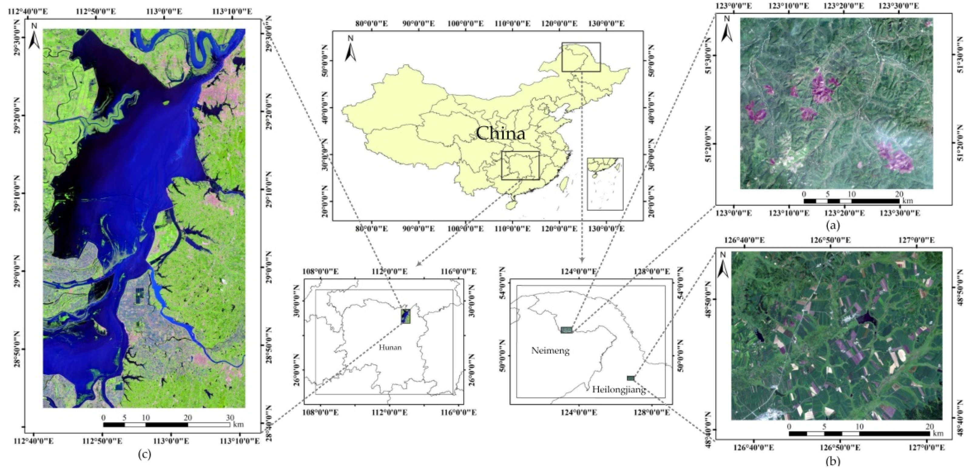
To evaluate the effectiveness and efficiency of the proposed FTMV fusion CD method, we considered three multispectral remote sensing datasets taken by different sensors with different changes and sizes, namely the Neimeng, Heilongjiang, and Hunan datasets (Figure 1).

Figure 1.
Location of the three used datasets in China: (a) Neimeng dataset, (b) Heilongjiang dataset, and (c) Hunan dataset.
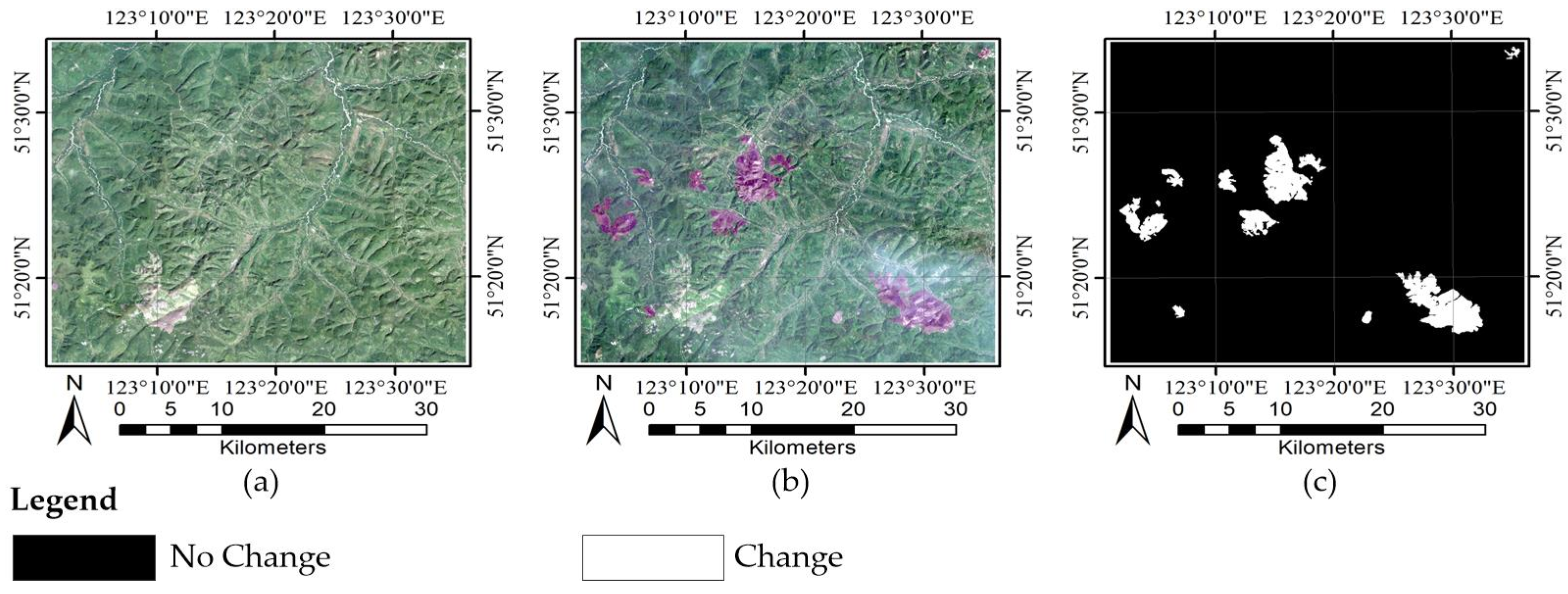
The Neimeng dataset consists of two Landsat-5 TM images acquired on the border of Neimeng and Heilongjiang Provinces on 22 August 2006 (T1) and 17 June 2011 (T2), respectively. A section of 1200 × 1350 pixels was selected for the experiments. These images display one main land cover types: forest. Between the two acquired times of the images, a wildfire (on 28 June 2010) destroyed a large portion of the forest in the studied region. Figure 2a–c exhibit the image taken in August, image taken in June, and their reference image of changes. The reference image (Figure 2c) of the Neimeng dataset was generated manually based on a detailed visual analysis of the two-temporal images (Figure 2a,b) using ENVI. For the other two datasets, the same method is used to create their reference images.
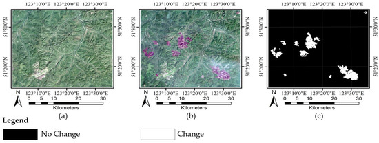
Figure 2.
Neimeng dataset: (a) Image of 2006; (b) image of 2011; and (c) reference image.
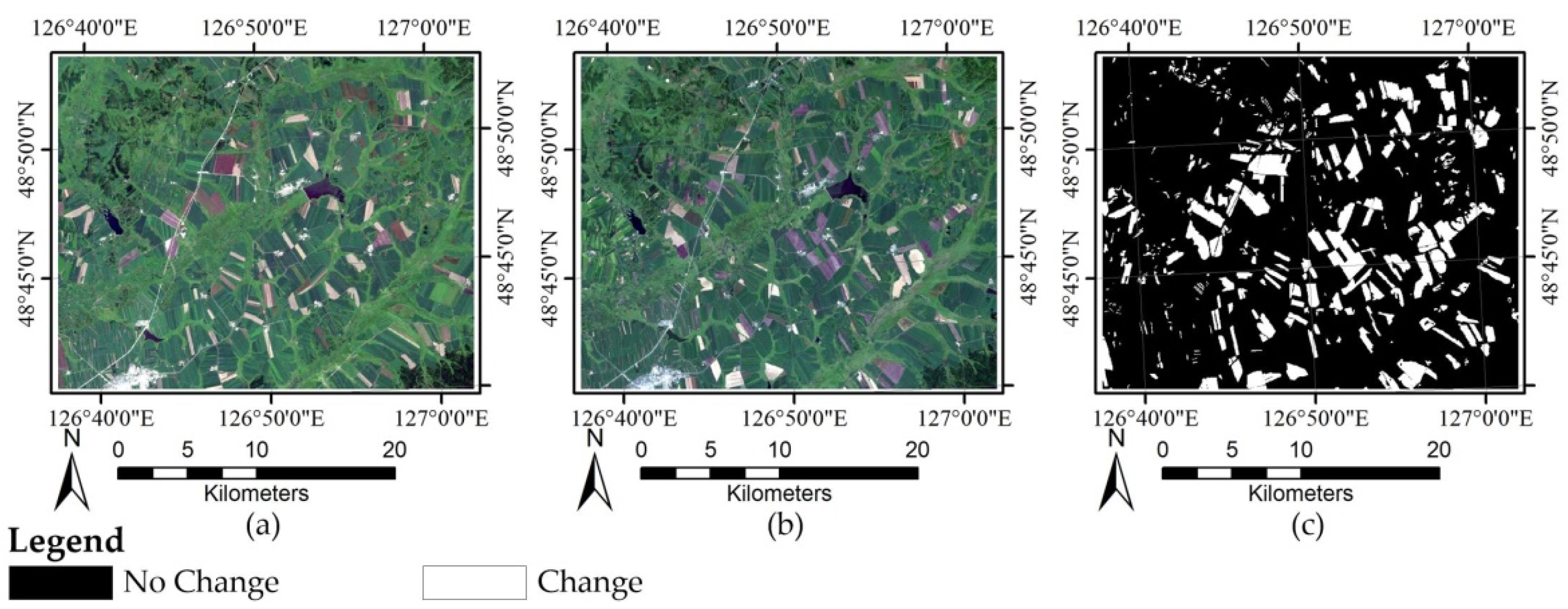
The Heilongjiang dataset comprises two Landsat-7 ETM+ images taken in Heilongjiang Province on 11 August 2001 (T1) and 14 August 2002 (T2), respectively. A typical area with 800 × 1000 pixels is selected as the test site. There are roughly two land cover types in these images: farmland and woodland. The changes occurred in the considered area during the study period mainly due to the new crop planting. The images of 2001 and 2002 are displayed in Figure 3a,b, respectively, and their reference image is displayed in Figure 3c.
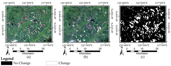
Figure 3.
Heilongjiang dataset: (a) Image of 2001; (b) image of 2002; and (c) reference image.
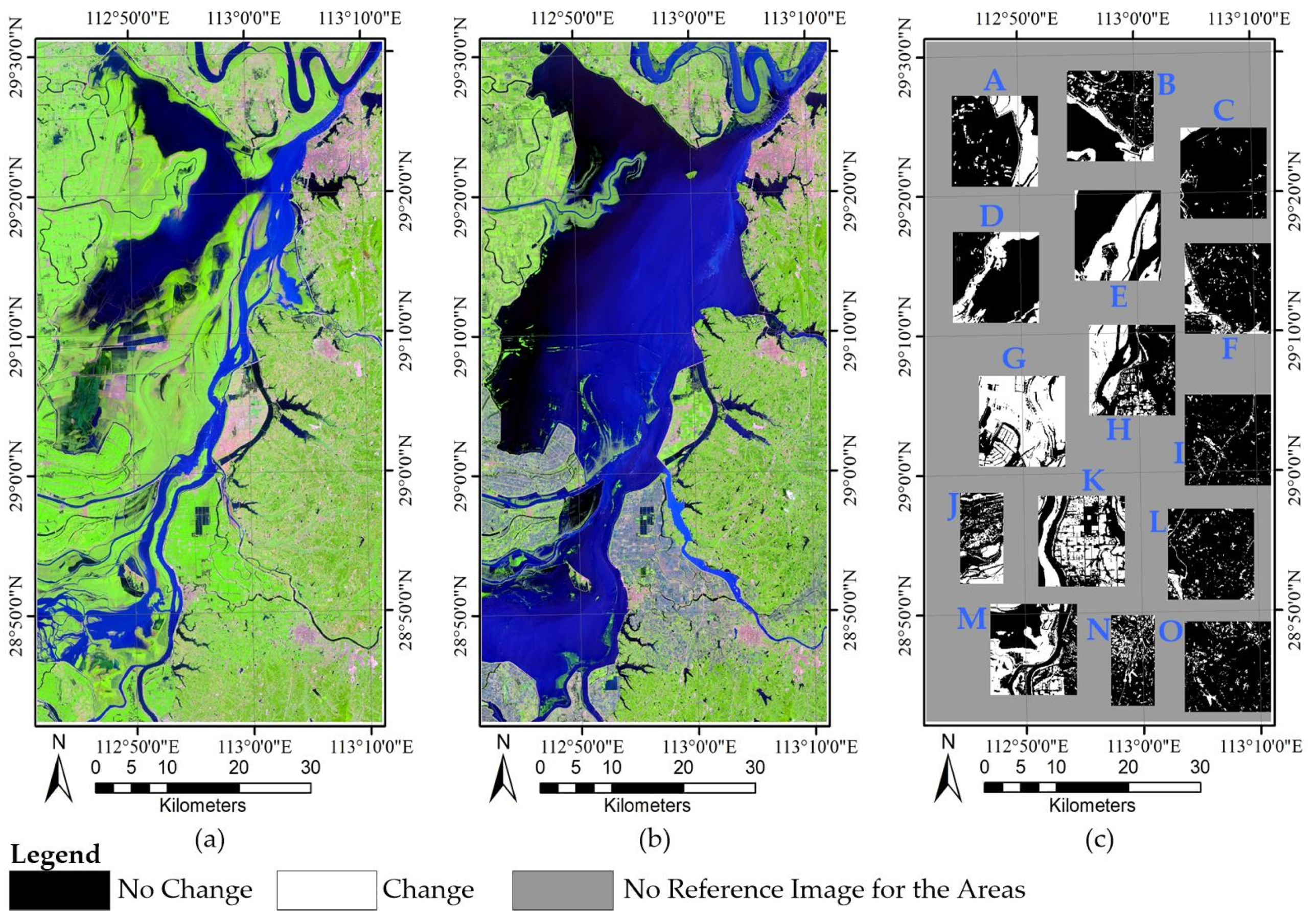
The Hunan dataset is made up of two Landsat-8 Operational Land Imager (OLI) images acquired in Hunan Province on 17 September 2013 (T1) and 23 July 2016 (T2), respectively. These images cover an area with a size of 3000 × 1600 pixels, and include four main classes: building, farmland, water, and woodland. The new crop planting, persistent rain, and urban construction in the study area introduced multiple kinds of change. Figure 4a,b display the images of 2013 and 2016, respectively.
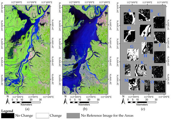
Figure 4.
Hunan dataset: (a) Image of 2013; (b) image of 2016; and (c) reference image.
For the Hunan dataset, it was more challenging to perform CD and very difficult to produce its reference image for the entire area because of its diversity of change types and larger geographical size. The sampling technique is one of the most important methods to evaluate the accuracy of algorithms, which has been widely used in CD studies (e.g., [11,19,24,26,27,28]). As such, we used the sampling technique to evaluate the performance of CD on the Hunan dataset. To achieve this, fifteen image blocks (Figure 4c) were selected according to stratified sampling. In particular, in order to guarantee the rationality of sampling and the accuracy of evaluation results, the samples were obtained by the following steps: First, the study area was stratified based on change types to ensure that the samples contain all the types of change. Then, fifteen image blocks that had a balanced space distribution were selected based on the stratified result. The obtained image blocks thus possess a balanced distribution in space and contain all the types of change. Figure 4c displays the reference image for the Hunan dataset: white represents the changed areas, black represents the unchanged areas, and grey indicates that there is no reference image in the corresponding areas.
The Neimeng and Heilongjiang datasets are used to test the effectiveness of the proposed FTMV CD method on single types of change (i.e., the forest change by a wildfire and farmland change by new crop planting). The Hunan dataset is used to test the effectiveness of FTMV for multiple types of change and larger geographical size, which is more challenging. To perform CD, co-registration and (relative) radiometric correction are two necessary preprocessing operations which will render the two-temporal images comparable in both the spatial and spectral domains [12,29]. For each dataset, the T2 image was first registered on the T1 one, and then the relative radiometric correction was performed on T2 image by referencing T1 image using the histogram matching method.
3. Proposed FTMV Fusion CD Method
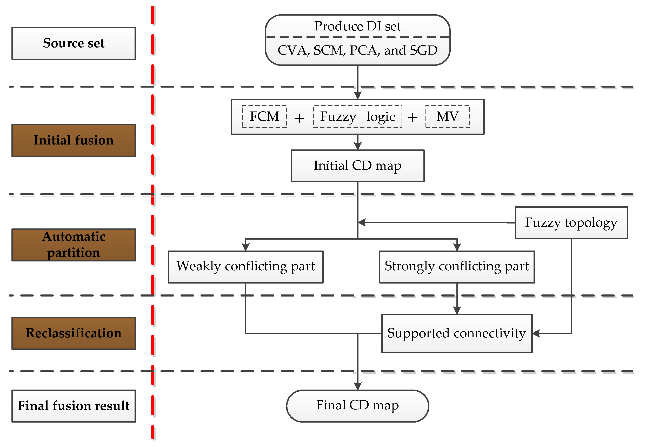
Let X1 and X2 denote two radiometrically corrected and co-registered multispectral remote sensing images acquired on the same ground area at two different times. A DI set with four elements providing complementary change information is produced for X1 and X2, as done in [24]. The four DI images are generated by the change vector analysis (CVA), spectral correlation mapper (SCM), principal component analysis (PCA), and spectral gradient differencing (SGD), respectively. The four DI images are denoted as CVA, SCM, PCA, and SGD. More details of producing the four DIs can be found in [24]. It should be noted that the DI set used in FTMV can be adjusted in practical applications.
After obtaining the DI images, the proposed FTMV fusion algorithm is applied to analyze and combine them. As illustrated in Figure 5 and Table 1, the FTMV fusion CD method includes three principal stages: (1) initial fusion; (2) automatic partition; and (3) reclassification. In the following, Section 3.1 introduces the mathematical basis for the proposed FTMV method. Section 3.2, Section 3.3 and Section 3.4 detail the three stages of FTMV.
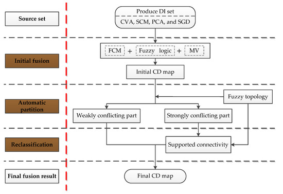
Figure 5.
Flowchart of the proposed FTMV CD technique.

Table 1.
The proposed FTMV CD technique.
3.1. Mathematical Basis for the Proposed FTMV
This section introduces three key concepts: fuzzy set, fuzzy topology, and fuzzy topological space, which form the mathematical basis of the proposed FTMV. Fuzzy set is a generalization of the classical set by introducing the concept of partial membership. Let us consider a nonempty universal set U and a complete lattice I = [0, 1]. A fuzzy set A on U is a mapping μA(x): U→I, where 0 ≤ μA(x) ≤ 1 for all the elements x in U. μA(x) is called the membership function of fuzzy set A.
Let IU be the family of all the fuzzy sets on U. That is, IU consists of all the mappings from U to I. Let δ be a subset of IU. Then, δ is called a fuzzy topology on U and the pair (U, δ) is called a fuzzy topological space if δ satisfies the following three conditions [30]:
- (1)
- Ø, U∈δ.
- (2)
- If A, B∈δ, then A∩B∈δ.
- (3)
- Let δ, where J is an index set, then ∈δ.
where Ø and U represent the empty set and whole set, and ∪ and ∩ denote the union operation and intersection operation of fuzzy sets.
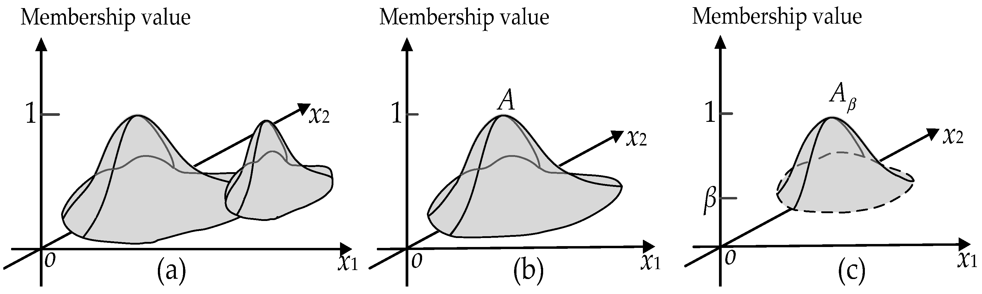
In a traditional three-dimensional geometric space, a point is represented by a three-dimensional vector (x1, x2, x3). That is, all the three dimensions x1, x2, and x3 are used to describe the location information of the point. Different from this, for a triple (x1, x2, μA(x1, x2)) in a three-dimensional fuzzy topological space (Figure 6a), only the first two dimensions x1 and x2 describe the location of a point, whereas the third dimension represents the membership degree of the point belonging to the set A. As a consequent, the general fuzzy topological space contains two structures of space: membership (levelling) structure and location (neighbourhood) structure. The two structures correspond to the membership-value axis and the x1-o-x2 plane of the coordinate system used, respectively. Fuzzy topology thus is a suitable tool to study and analyze both the membership structure and neighbourhood structure of spaces.
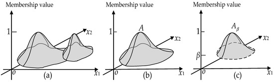
Figure 6.
Examples of a fuzzy topological space and a level cut interior operator: (a) A simple example of a three-dimensional fuzzy topological space; (b) Fuzzy set A; and (c) Interior Aβ of fuzzy set A.
According to [30], fuzzy topology can be defined by the interior operator, which, in turn, can be defined by a suitable level cut. Let us consider a fuzzy set A with a membership function μA(x); for a fixed value β∈(0, 1), we can define a level cut interior operator Aβ (Figure 6b,c) as follows:
The level cut interior operator Aβ can induce a fuzzy topology (termed as LC fuzzy topology). Using LC fuzzy topology to analyze its membership function, a fuzzy set A can be divided into two parts: interior Ao and fuzzy boundary ∂A:
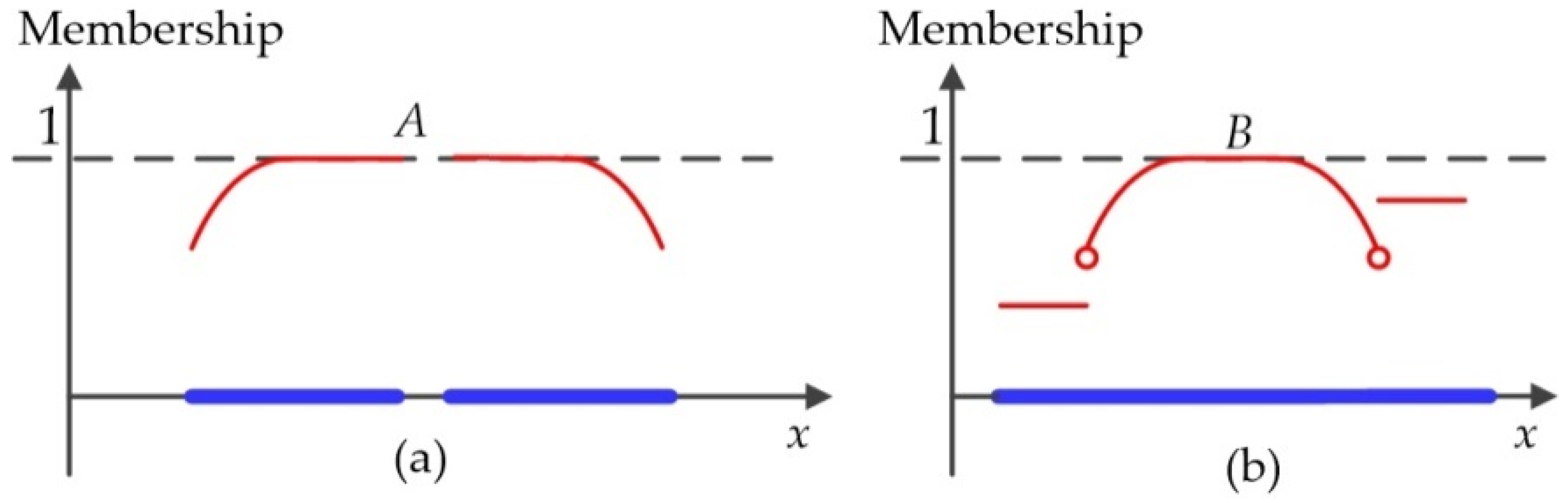
As an important characteristic of fuzzy topology, the connectivity of fuzzy spatial objects in a fuzzy topological space includes two types of structure: membership and location connectivity of points. Figure 7 presents two examples of fuzzy spatial objects in a two-dimensional fuzzy topological space: Object A (Figure 7a) is membership connected but location disconnected, whereas Object B (Figure 7b) is location connected but membership disconnected.
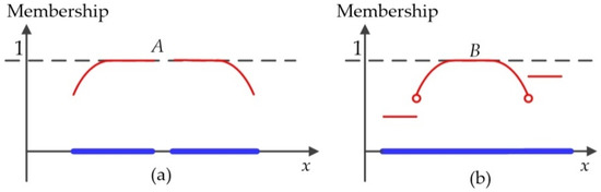
Figure 7.
Two examples of fuzzy spatial objects in a two-dimensional fuzzy topological space: (a) An example of a membership connected but location disconnected object and (b) an example of a location connected but membership disconnected object.
In this study, we define the decision-level fusion CD problem in terms of fuzzy topology, in which the changed and unchanged classes are regarded as fuzzy sets. In particular, the initial fusion and automatic partition stages of the proposed FTMV approach are realized by analyzing the membership structure of fuzzy topological space, whereas the reclassification stage is achieved by analyzing the location structure. We refer to [30] for more details on the fuzzy topological space.
3.2. Initial Fusion
MV is a simple but effective decision-level fusion technique and has been applied successfully in many fields. The main idea of MV is to combine the output results obtained from different data sources using the majority voting rule [11].
Let us consider an n-class (Cj, j = 1, 2, …, n) classification problem for which m different data sources are available. For a given sample x, let yi(x) = {yi1(x), yi2(x), …, yij(x), …, yin(x)} denote its classification result obtained based on source Si (i = 1, 2, …, m, j = 1, 2, …, n), where yij(x) is a binary valued function, defined as follows:
Let Vj(x) denote the number of votes of sample x to class Cj (j = 1, 2, …, n) received from the m data sources. Then, Vj(x) can be computed as follows:
According to the majority voting rule, the sample x is assigned to the class Ck with the largest number of votes as the consensus decision [31]:
As shown in Equations (3)–(5), the conventional MV is based on the classical set theory, and makes decision by combining the binary valued class vectors (i.e., yi(x)). However, using binary valued vectors for fusion may cause unreasonable fusion results in some cases.
3.2.1. Improve MV Using Fuzzy Logic
Let us consider a two-class (C1 and C2) classification problem for which four sources Si (i = 1, 2, 3, 4) are available. Suppose that dij(x) is the individual decision value (i.e., membership value or probability) according to source Si with respect to class Cj (j = 1 or 2) for a given sample x, and
d11(x) = d21(x) = d31(x) = 0.49, d41(x) = 0.95.
d12(x) = d22(x) = d32(x) = 0.51, d42(x) = 0.05.
Then, the classification results yi(x) = {yi1(x), yi2(x)} can be obtained by comparing the decision values di1(x) and di2(x): and , i = 1, 2, 3, 4. Thus,
y11(x) = y21(x) = y31(x) = 0, y41(x) = 1.
y12(x) = y22(x) = y32(x) = 1, y42(x) = 0.
According to Equations (4) and (5), for sample x, the final decision by MV will be in favour of class C2 following the classification results y1(x), y2(x), and y3(x) (from sources S1, S2, and S3). Nevertheless, for sources S1, S2, and S3, their decision values to classes C1 and C2 (0.49 and 0.51) are very close, causing their classification results to be very unreliable. On the contrary, the classification result from source S4 is of high confidence (reflected by the large difference between the d41- and d42-values). Therefore, it is more reasonable to assign x to C1 as the final decision by synthetically considering all four sources. The main reason for MV resulting in an unreasonable fusion result is that MV uses the binary (discrete) class label values yij(x) for voting.
To resolve this problem, we can use the continuous decision values dij(x) to replace the binary class label values yij(x) for voting during MV fusion. This is because the difference between the continuous decision values can reflect the reliability in the source decision to some extent. By doing so, we will obtain continuous votes to classes C1 and C2, i.e., V1(x) = d11(x) + d21(x) + d31(x) + d41(x) = 2.42, and V2(x) = d12(x) + d22(x) + d32(x) + d42(x) = 1.58. According to Equation (5), MV will decide class C1 and therefore yield a more reasonable fusion result.
Given the above analysis, we choose to use the continuous decision values for voting in MV, to compensate its drawback in this study. As a consequence, Equation (4) is rewritten as follows:
where dij(x) represents the decision value of sample x to class Cj according to source Si. In this work, the modified MV that performs fusion using continuous decision values is termed as fuzzy MV (FMV).
3.2.2. Analyze DI Images
In our case, there are two classes to be identified: the change class Cc and no-change class Cu. Four DI images serve as the four data sources: CVA, SCM, PCA, and SGD. Therefore, m = 4 and n = 2. We firstly analyze the DI images to determine each data source’s individual decision values.
In general, the ranges of DI pixel values belonging to the changed and unchanged categories have overlap, and therefore the pixels from these two categories are not separable by sharp boundaries [5]. Analyzing DI bears some inherent uncertainty. Fuzzy clustering is an appropriate method to analyze the DI, because of its robust characteristics for uncertainty. The pixels of DI in fuzzy clustering are not assigned to class Cc or class Cu, but to both classes with certain membership degrees [4].
In particular, we apply the widely used fuzzy clustering algorithm FCM to analyze the DIs for calculating their membership functions (also called fuzzy partition matrix). Then, the individual decision values dij(x) for the four DI sources are derived according to the membership functions computed by FCM. More details of FCM can be found in [32].
3.2.3. Generate an Initial Fusion CD Map by FMV
Let Ui = {uij(x)} denote the fuzzy membership functions obtained by FCM according to the ith DI, i =1, 2, 3, 4, j = u, c. Here uij(x) represents the membership degree for pixel x with respect to class Cj obtained based on the ith DI, and satisfies
The individual decision values of each DI source are then defined using Ui. For a given pixel x, its decision value with respect to class Cj from the ith DI, dij(x), is given as follows:
After obtaining dij(x) (i = 1, 2, 3, 4, j = u or c), the votes of pixel x to class Cj (j = u or c), Vj(x), are computed using Equation (6). An initial CD map is produced according to the majority voting rule expressed by Equation (5). Let L(x) denote the class label of pixel x, and it is given by
3.3. Automatic Partition
The modified MV (i.e., FMV) can largely overcome the drawback of MV caused by using binary class label values, but it may still lead to unreliable CD results for the pixel patterns with strong conflicts. For example, let us consider a pixel xA with the following individual decision values:
d1u(xA) = d2u(xA) = 0.03, d3u(xA) = d4u(xA) = 0.98.
d1c(xA) = d2c(xA) = 0.97, d3c(xA) = d4c(xA) = 0.02.
Then, using Equation (6), we can obtain Vu(xA) = 2.02 and Vc(xA) = 1.98, and the pixel xA is assigned to class Cu according to Equation (9).
The decision values of pixel xA to classes Cu and Cc from every DI source (namely diu(xA) and dic(xA)) are significantly different. Thus, the decision of each DI source at pixel xA has high confidence. However, the four sources at xA have strong conflicts: sources 1 and 2 are in favour of class Cc, whereas sources 3 and 4 in favour of class Cu. As a result, the votes of pixel xA to classes Cu and Cc (Vu(xA) = 2.02 and Vc(xA) = 1.98) are very close, which means the CD result of xA by FMV has high uncertainty.
The above analysis shows that, for the strongly conflicting pixels, FMV may lead to questionable CD results. Many pixels with strong conflicts are often misclassified in the initial fusion CD map created by FMV. To resolve this problem, this study adopts fuzzy topology to further improve the initial CD result. Firstly, the strongly conflicting pixels are determined by analyzing the membership structure of the FMV fusion result. Then, the determined pixel patterns are reclassified by reconstructing their neighbourhood structure, using the supported connectivity of fuzzy topology.
3.3.1. Partition the Initial Fusion CD Map Conceptually
Let FSu and FSc represent the sets that are composed of the unchanged and changed pixels in the initial CD map produced by FMV:
And let Conu and Conc denote the sets consisting of the strongly conflicting pixels in FSu and FSc, respectively.
The difference between the votes Vu(x) and Vc(x) can reflect the four DI sources’ conflict degree at pixel x to a certain extent. The smaller the difference is, the more conflicting the four sources are. The conflict degree reaches the maximum when Vu(x) and Vc(x) are equal, i.e., Vu(x) = Vc(x) = 2.
If we normalize Vj(x) (j = u, c) using Equation (11), they will satisfy: 0 ≤ Vj(x) ≤1 and Vu(x) + Vc(x) = 1. Then, the normalized function Vj(·) (j = u or c) can be regarded as a membership function of FSj, and FSj can be regarded as a fuzzy set in fuzzy topological space.
In addition, the difference between the normalized Vu(x) and Vc(x) can still reflect the conflict degree of the four DI sources at pixel x. Given that the smaller the difference, the more conflicting the sources, 0 ≤ Vj(x) ≤ 1, and Vu(x) + Vc(x) = 1, it is easy to obtain the following property.
Property 1.
For each pixel x, the closer the Vj(x)-value (j = u or c) is to 0.5, the more conflicting the four DI sources are, and the conflict degree of sources will reach to the maximum when Vu(x) = Vc(x) = 0.5.
Accordingly, the strongly conflicting pixel set Conj (j = u or c) can be determined by analyzing the membership structure of the fuzzy set FSj using fuzzy topology. In particular, we use the LC fuzzy topology (Section 3.1) to analyze the fuzzy set FSj, which is partitioned conceptually into two parts: interior and fuzzy boundary ∂FSj:
where βj is a constant and βj∈(0.5, 1). Obviously, the Vj(x)-values of the pixels in the fuzzy boundary ∂FSj are close to 0.5. According to Property 1, the pixels in ∂FSj are of strong conflicts. Thus, we use the fuzzy boundary ∂FSj to define the strongly conflicting pixel set Conj:
As a result, the initial CD map yielded by FMV is conceptually divided into two parts: strongly conflicting part Conu ∪ Conc and weakly conflicting part ∪.
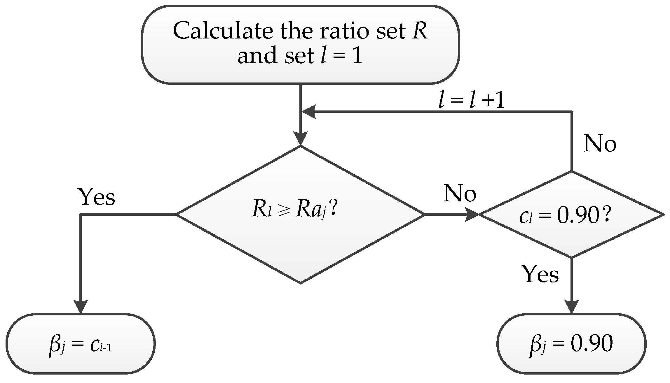
3.3.2. Determine the Optimal Threshold βj
The key to recognizing the strongly conflicting pixels is to determine the optimum threshold βj for FSj, j = u or c. An automatic and adaptive method is proposed in this study for searching the optimum βj. As 0.5 < βj < 1, the search range is set as (0.5, 1). Two main factors need to be taken into consideration to set the search pace: (1) The optimum threshold may be missed if the search pace is too large; (2) the computational complexity may be too high if the search pace is very small. Considering both the two factors, we propose setting the searching pace as 0.05, and search the optimum βj in the candidate set C = {0.55, 0.60, 0.65, 0.70, 0.75, 0.80, 0.85, 0.90}.
According to Property 1, the closer the Vj(x)-value is to 1, the weaker the conflict and the more reliable the FMV CD result of pixel x. From this perspective, the βj-value should be as large as possible. On the other hand, the larger the βj-value is, the more pixels the strongly conflicting pixel set Conj has. However, the final CD accuracy will be affected negatively if there are too many recognized strongly conflicting pixels in Conj. In general, the uncertain pixels likely to be misclassified in DI account for about 15% of the total pixels [7]. Denote the upper bound of the percentage of the strongly conflicting pixels in FSc by Rac, and that in FSu by Rau. A higher Rac or Rau value helps to recognize the strongly conflicting pixels in DI. However, a higher Rac and Rau also may increase missed detection errors and false alarm errors, respectively, in the subsequent reclassification. The meanings of missed detection errors and false alarm errors can be seen in Section 4.1. In most cases, the no-change area in DI is far larger than the change area. Thus, a higher Rac value for FSc is more risky and may lead to serious missed detection errors, while a higher Rau value for FSu is more beneficial for recognizing the strongly conflicting pixels. Accordingly, Rac is set to 10% and Rau is set to 20%.
Given the above analysis, we present an automatic and adaptive method to search the optimum βj (Figure 8), termed as AAM, which consists of three main steps:

Figure 8.
Flowchart of searching the optimal βj.
Step 1: Calculate the ratio set R = {Rl | Rl = nl/n} and set l = 1. n and nl stand for the numbers of the pixels in FSj and the set {x | 0.5 < Vj(x) < cl}, respectively. cl = 0.5 + 0.05 × l belongs to the candidate set C, l = 1, 2, 3, 4, 5, 6, 7, 8.
Step 2: If Rl ≥ Raj (j = u or c), then stop and let βj = cl-1, otherwise go to Step 3. Here Rau = 20%, Rac = 10%, and c0 = 0.5.
Step 3: If cl = 0.90 then stop and let βj = 0.90, otherwise set l = l + 1 and go to Step 2.
The proposed searching approach AAM is to find the maximum cl that satisfies Rl < Raj from the candidate set C. The found cl can ensure that 1) the βj-value is as large as possible and 2) the recognized strongly conflicting pixels are within a reasonable range.
3.4. Reclassification
The initial fusion CD map by FMV has been partitioned into two parts in Section 3.3 by analyzing the membership structure of the fuzzy set FSj (j = u and c): strongly conflicting part Conu∪Conc and weakly conflicting part ∪. The pixels in the weakly conflicting part have little or no conflict. FMV has a good performance on classifying such pixels, so their CD results by FMV are taken as their final detection results. That is, the pixels in and are finally assigned to classes Cc and Cu, respectively. For the pixels in Conu∪Conc, FMV often generates problematic CD results, so they need to be reclassified. A possible approach to reclassify the strongly conflicting pixels is to utilize the spatial connectivity, since the spatial objects are usually spatial-location (neighbourhood) connected.
As shown in Section 3.1, the connectivity in fuzzy topological space includes membership connectivity and location connectivity of points. The former corresponds to the membership domain of points (or pixels), whereas the latter corresponds to the spatial-location domain. The pixels in an image are usually highly correlated with their neighbors. The connectivity of spatial objects therefore mainly depends on the spatial-location structure of points. In order to describe and model the spatial-location (neighbourhood) connectivity of points in fuzzy topological space, the concept of supported connectivity was developed in [30]. The supported connectivity provides a suitable tool to process the fuzzy boundary (i.e., strongly conflicting) pixels.
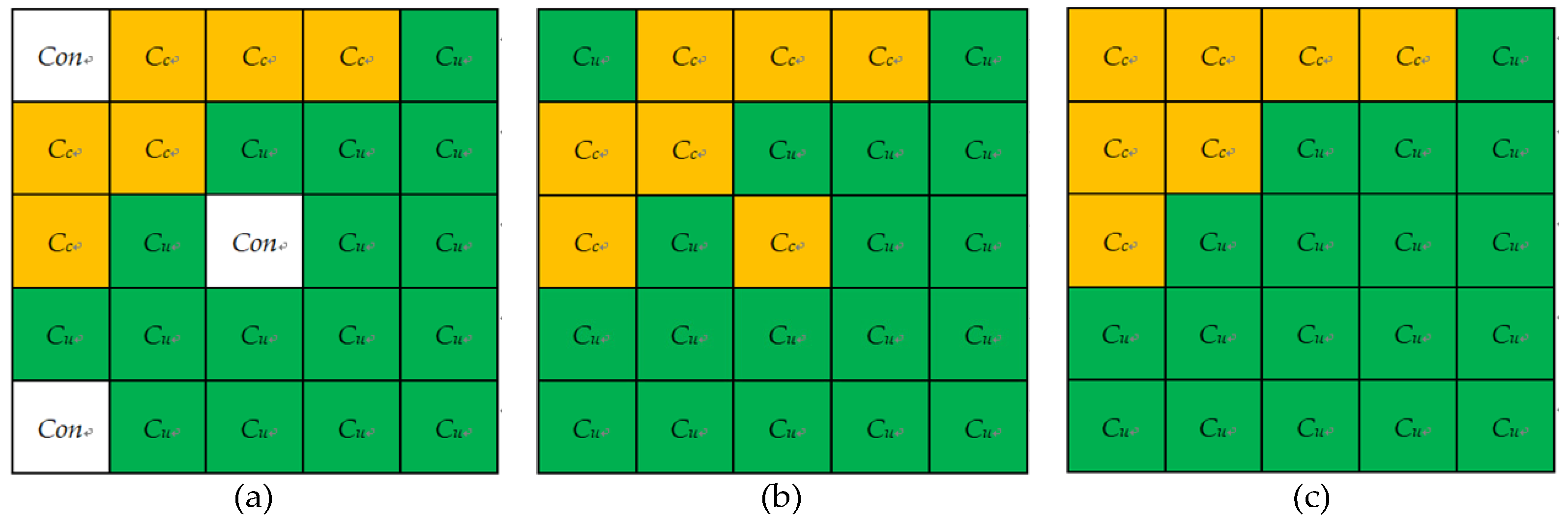
This study presents a simple but effective method to reclassify the recognized strongly conflicting pixels based on the supported connectivity. The main idea of the method is to search the neighbourhood window of each strongly conflicting pixel and utilize the already labelled neighbouring pixels in the window to reclassify the center pixel of the window. Figure 9a presents an example of a 5 × 5 neighbourhood window for a strongly conflicting pixel. Cu (Cc) means that the pixel has been already labelled as class Cu (Cc). Con indicates that the pixel has strong conflicts remaining to be relabeled. The operational procedure of reclassifying the pixels with strong conflicts includes three steps:

Figure 9.
An example of the changes in topology relations in a 5 × 5 neighbourhood window: (a) Partition result by fuzzy topology of (b); (b) CD result of FMV; and (c) CD result after reclassification.
Step 1: Search the location of all the strongly conflicting pixels.
Step 2: For each strongly conflicting pixel x0, search its (2R + 1) × (2R + 1) neighbourhood window and record the already labelled neighbouring pixels in the window, then the pixel x0 belongs to the class already assigned to the larger number of neighbouring pixels. When the pixel x0 is totally surrounded by the strongly conflicting ones, it will be assigned to class Cc if Vc(x0) ≥ Vu(x0), or to class Cu otherwise.
Step 3: Repeat Step 2 until all the pixels with strong conflicts have been reclassified.
The automatic partition described in Section 3.3 breaks down the topology relations (e.g., the boundary, membership connectivity, and location connectivity) of fuzzy set FSj (j = u or c), which are reconstructed in the reclassification process. Figure 9 shows an example of the changes in topology relations caused by the automatic partition and topology relation reconstruction. The old boundary and location connectivity relations of classes Cu and Cc (Figure 9b) are broken down by the partition process (Figure 9a), and new boundary and location connectivity relations (Figure 9c) are constructed after reclassification. The Con pixels are relabeled into either Cu or Cc, as shown in Figure 9c.
4. Results
4.1. Experiment Setup and Evaluation Criteria
In order to evaluate the performance of the proposed FTMV CD method, eleven CD techniques in three types were used as comparative methods (Table 2).
Table 2.
Comparison methods used in this study.
In the four single-DI detectors, the CD results were produced by respectively clustering the CVA, SCM, PCA, and SGD DI images with FCM. In the HFV approach, after producing the hybrid DI, the CD was also performed by FCM. FLICM and RFLICM were implemented on the DI produced by the most frequently used CVA technique. The weighting exponent used in FCM, FLICM, and RFLICM was set to 2. The other parameters involved in the approaches were determined according to the trial-and-error procedure. Only the best detection results of each approach were given for the evaluation and illustration of performance.
The CD performance was evaluated based on four accuracy indices: missed detections (MD), the number of changed pixels that are identified as unchanged ones; false alarms (FA), the number of unchanged pixels that are identified as changed ones; overall error (OE), the sum of MD and FA, OE = MD + FA; and Kappa coefficient (KC), which are widely used in the CD studies (e.g., [5,12,19,23,24,34]). KC is computed by
where N represents the number of the pixels in the CD map, and NU and NC denote the correctly detected no-change and change pixels. MD and FA are two specific criteria for evaluating the performance of CD and their importance dependence on the practical application, whereas OE and KC are two global criteria. KC is more cogent than other indices since it involves more classification information [35,36]. Additionally, the consumption time T of each algorithm was also recorded for the comparison of time complexity. The eleven comparative algorithms and the proposed FTMV were all carried out in a computer that has Intel(R) Core(TM) i7-9750H 2.59 GHz processor and 16 GB RAM.
4.2. Experiment Results
Figure 10 and Figure 11 illustrate the CD maps produced by different algorithms for the Neimeng dataset. Figure 12 and Figure 13 show the CD maps for the Heilongjiang dataset. To illustrate the difference between the CD maps and the corresponding reference image clearly, each CD map was divided into four parts: black and white represent the correctly detected no-change and change pixels, whereas red and yellow denote the MD and FA pixels. For the Hunan dataset, it is too large to clearly exhibit the detailed information of its CD maps in one page. Moreover, the experiment on the Hunan dataset agrees with the results of the other two datasets, so we only present the two best CD maps obtained by DSK and FTMV for the Hunan dataset (Figure 14). Table 3, Table 4 and Table 5 summarize the five quantitative indices (i.e., MD, FA, OE, KC, and T) of each CD algorithm on the Neimeng, Heilongjiang and Hunan datasets.

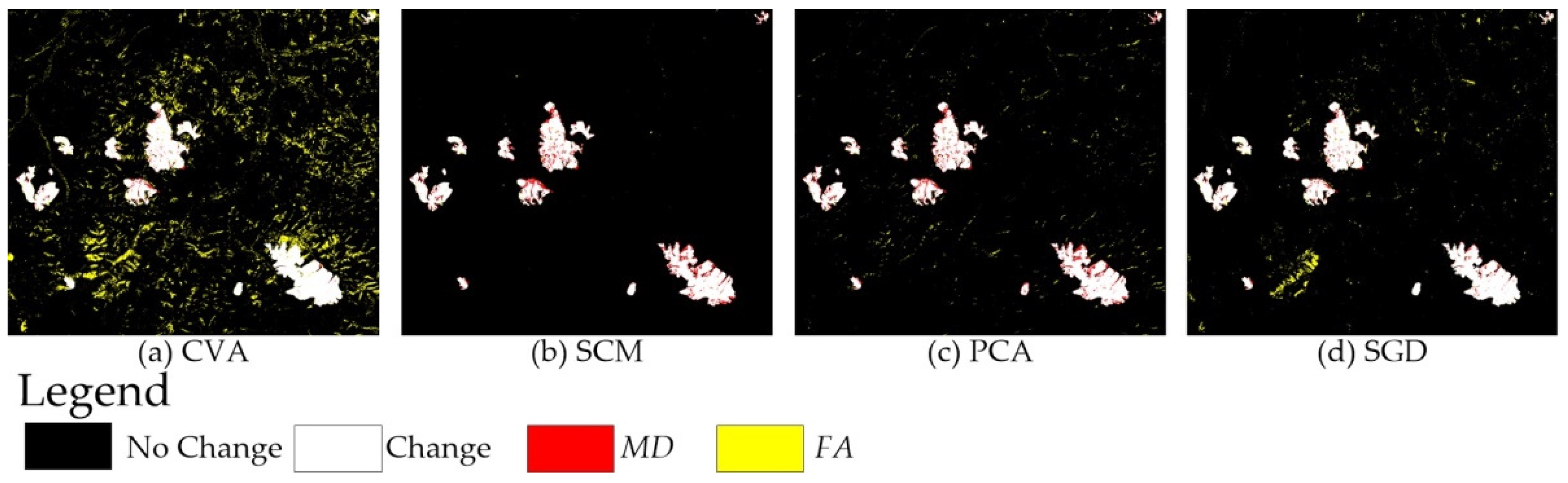
Figure 10.
CD maps created by the four single-DI detectors on the Neimeng dataset.
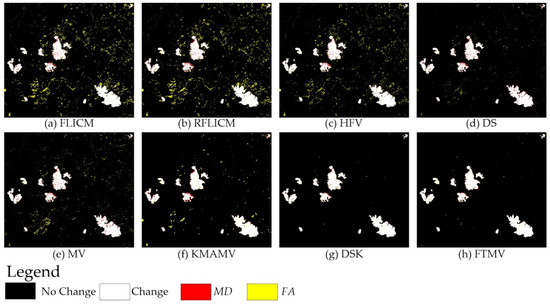
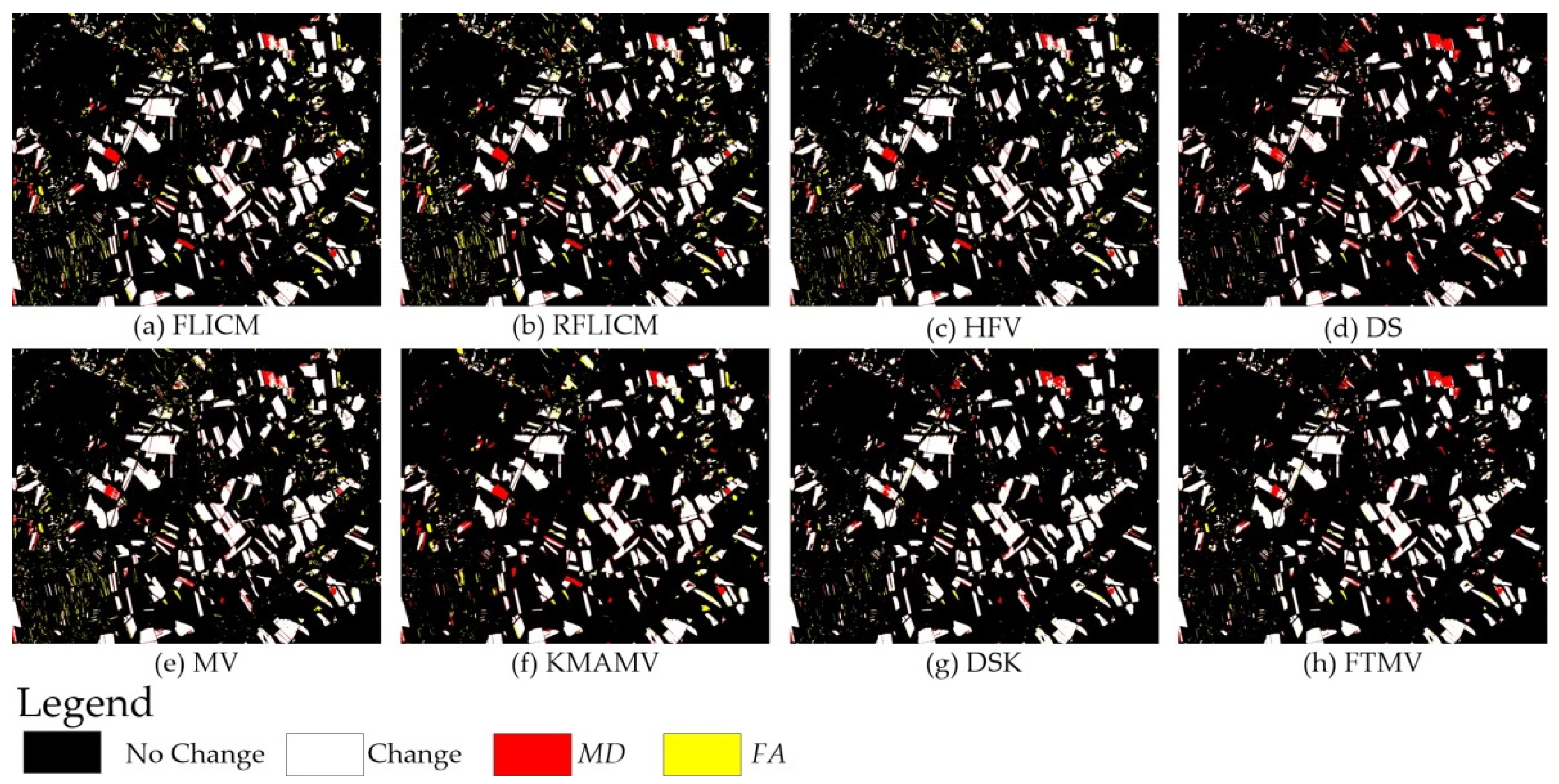
Figure 11.
CD maps created by the other eight methods on the Neimeng dataset.
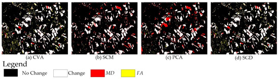
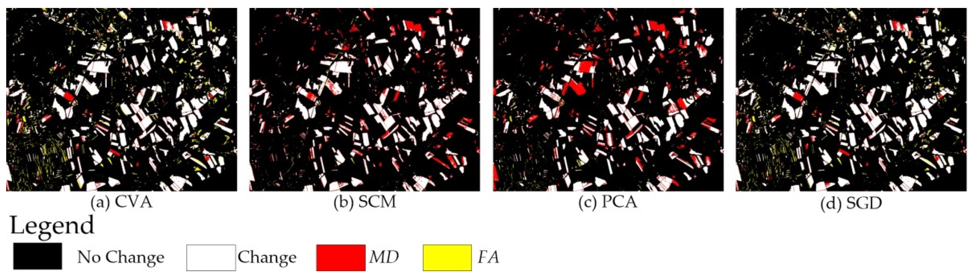
Figure 12.
CD maps created by the four single-DI detectors on the Heilongjiang dataset.
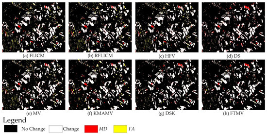
Figure 13.
CD maps created by the other eight methods on the Heilongjiang dataset.
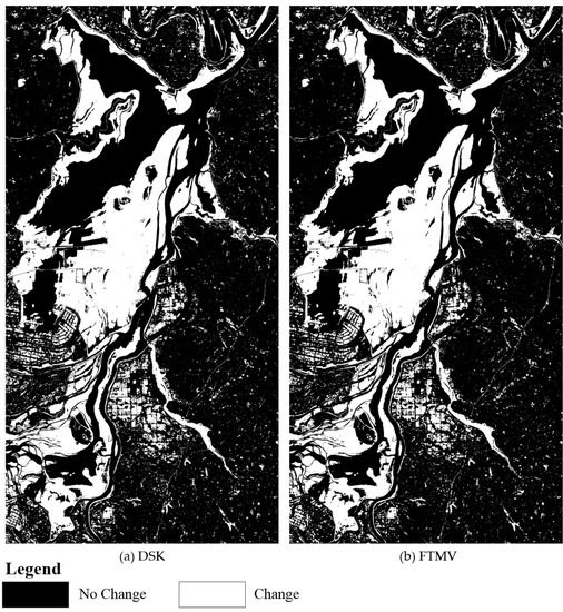
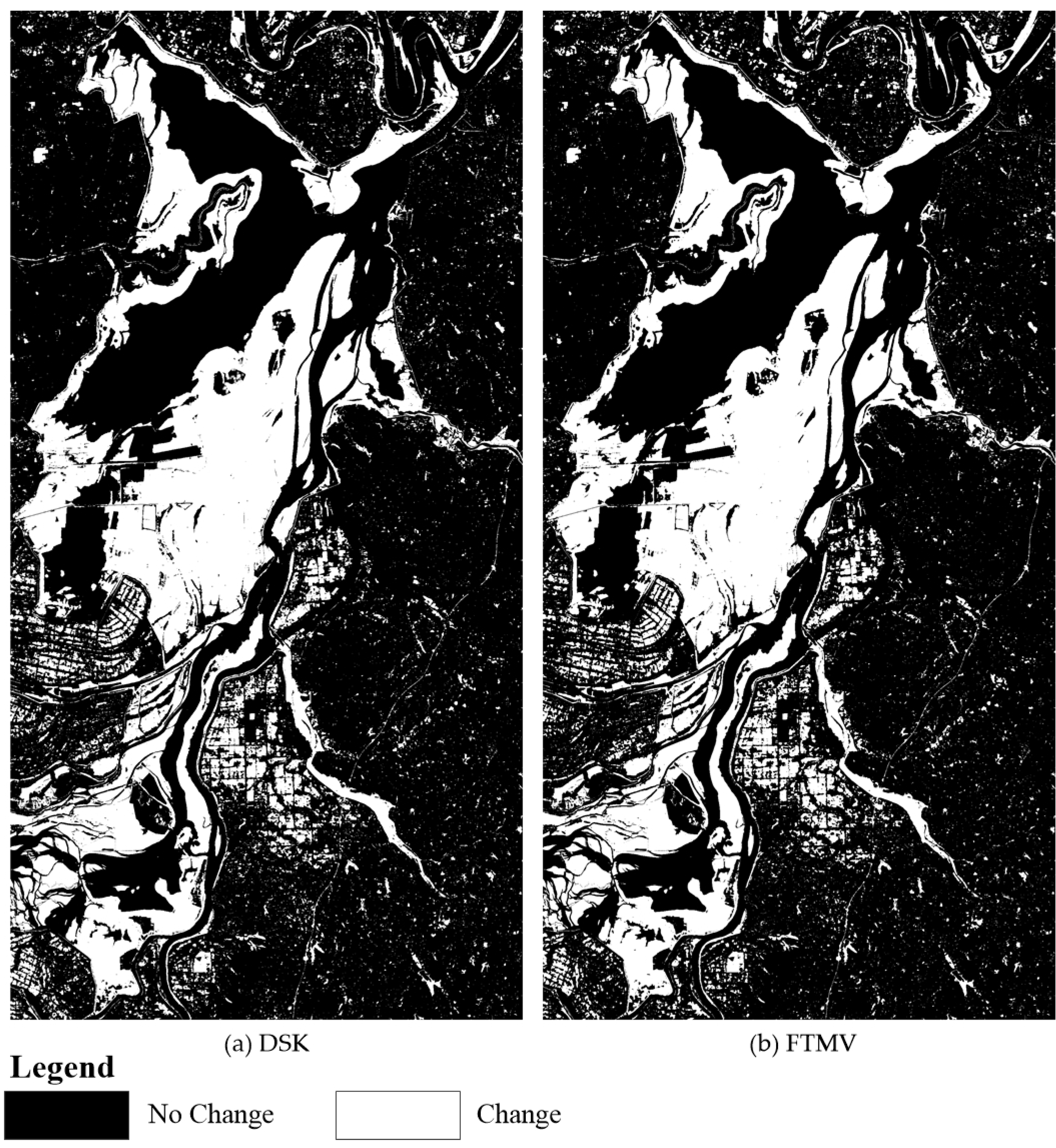
Figure 14.
CD maps created by DSK and FTMV on the Hunan dataset.
Table 3.
Quantitative evaluation indices of the Neimeng dataset.
Table 4.
Quantitative evaluation indices of the Heilongjiang dataset.
Table 5.
Quantitative evaluation indices of the Hunan dataset.
Figure 10 and Figure 11 and Table 3 show the qualitative and quantitative comparisons of the CD results provided by different methods of the Neimeng dataset, respectively. Four individual DI detectors created varied but complementary CD maps (Figure 10): The CD maps produced by CVA and SGD have many scattered noise pixels (yellow areas) but few MD errors (red areas), whereas the change map yielded by SCM contains few yellow areas of FA but large red MD areas. This demonstrates the potential for improving the CD performance of single-DI detectors by performing fusion techniques. SCM achieves the best CD results amongst the four individual detectors for the first dataset (Table 3).
For the other seven comparative approaches, FLICM, RLFICM, HFV, and MV generate better CD maps (Figure 11a–c,e) than CVA, but their maps still contain many yellow noise pixels. The CD maps produced by KMAMV and DS are better than those from FLICM, RLFICM, HFV, and MV (Figure 11). However, the maps of KMAMV and DS (Figure 11f,d) are not satisfactory enough in comparison to the reference change image. There still exist apparent scattered yellow FA pixels and a few red MD areas.
The benchmark algorithm DSK (Figure 11g) produces the most accurate CD results among the eleven comparative algorithms, as shown in Figure 10 and Figure 11 and Table 3. Nevertheless, DSK suffers from two serious drawbacks [24] which limit its application: (1) DSK is sensitive to the two key threshold parameters used to recognize the strongly conflicting pixels and requires repeated tuning of them. It is quite laborious and affects the automation level of DSK; and (2) DSK needs to calculate experimental covariance functions for using indicator kriging (to reclassify the pixels with strong conflicts), which is time-consuming and leads to the high computational complexity of DSK.
By introducing MV into fuzzy topological space, the proposed FTMV approach can combine the CD results from different DIs and largely resolve the conflicting problem during fusion. It achieves significantly better CD results than the first ten benchmark CD algorithms (Figure 10 and Figure 11, and Table 3). For example, the KC value resulted from FTMV is 0.9590, which is 35.53%, 5.23%, 8.82%, 7.38%, 23.18%, 24.91%, 16.15%, 5.41%, 9.36%, and 5.79% larger than CVA, SCM, PCA, SGD, FLICM, RFLICM, HFV, DS, MV, and KMAMV, respectively.
By comparing with DSK, it is proved that the proposed FTMV method not only overcomes the two shortcomings of DSK, but also provides an result with as good accuracy as DSK. Specifically speaking, FTMV develops an automatic approach to determine the strongly conflicting pixels, whereas DSK requires repeated tuning of two key threshold parameters, thus FTMV has a higher degree of automation and is more feasible in practical applications. Additionally, FTMV reclassifies the recognized strongly conflicting pixels by connectivity analysis, which avoids computing the experimental covariance functions required in DSK. Consequently, the computation time of the proposed FTMV is obviously reduced compared with DSK, as shown in Table 3. It should be pointed out that the recorded time of DSK (in Table 3, Table 4 and Table 5) only contains its execution time, without the time of manually tuning the two key threshold parameters. The advantages of FTMV over DSK are further discussed in Section 5.3.
As shown in Figure 12 and Figure 13 and Table 4, the CD maps provided by the four single-DI detectors are also complementary for the Heilongjiang dataset (Figure 12): The change maps yielded by CVA and SGD have small red MD areas, whereas the maps from SCM and PCA include few yellow FA errors. SGD performs best amongst the four individual detectors. FLICM and RFLICM generate slightly worse CD results (Figure 13a,b), whereas HFV, DS, MV, and KMAMV produce slightly better CD results (Figure 13c–f), in comparison to SGD (Figure 12d). Again, FTMV and DSK achieve the CD maps (Figure 13g,h) closest to the corresponding reference image, demonstrating their highest accuracy. Compared with DSK, the proposed FTMV CD algorithm achieves nearly identical accuracy but in a more efficient and automated manner (as shown in Table 4 and Section 5.3).
The quantitative indicators obtained by different algorithms on the Hunan dataset (Table 5) were computed according to the fifteen selected image blocks (Figure 4c). As reported in Table 5, CVA achieves the lowest OE and highest KC for the four single-DI detectors. FLICM, RFLICM, HFV, DS, MV, and KMAMV show slightly better performance than CVA. For the Hunan dataset, which is quite challenging, FTMV and DSK also produce the best and almost the same accuracy CD results. On the other hand, the proposed FTMV method outperforms DSK in terms of both efficiency and automation (Table 5 and Section 5.3).
5. Discussion
5.1. Robustness of Neighbourhood Window Size
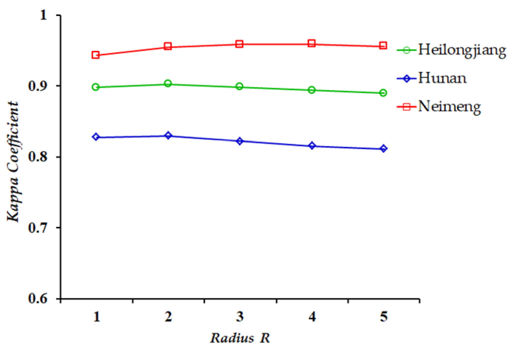
There is only one parameter (i.e., the parameter R used to control the neighbourhood window size) that needs to be set in the proposed method. This subsection discusses the robustness of parameter R. To this end, R was set to 1, 2, 3, 4, and 5, and the cogent KC-criterion was applied to assess the CD performance.
Figure 15 shows the change trends of the KC-values versus the parameter R for the three datasets. For all three cases, the KC-value increases slowly at first and then decreases slightly when the parameter R increases from 1 to 5. The KC-values are stable for various R-values in the set {1, 2, 3, 4, 5}. The stability demonstrates that the proposed FTMV is robust to the parameter R to a large extent. For all the three used datasets, one can choose any value from the set {1, 2, 3, 4, 5} to achieve a promising KC-value of FTMV.
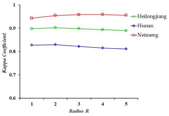
Figure 15.
Relationship curves between KC-values and parameter R.
5.2. Effectiveness of the Proposed AAM
This study proposes an automatic and adaptive method (i.e., AAM) to determine βu and βc, which are used in fuzzy topology for automatically recognizing the strongly conflicting pixels. To evaluate the effectiveness of AAM, experimental studies were carried out on the three used datasets. Table 6 presents the βu- and βc-values achieved by the proposed AAM and their optimal values. The optimal βu- and βc-values were obtained by parameter tuning. We changed βu and βc from 0.5 to 1 with an incremental step size of 0.01. The cogent KC was used as the criterion.
Table 6.
Values of βu and βc achieved by the proposed AAM and their optimal values.
As shown in Table 6, the proposed AAM provides almost optimal results for all three cases: The βu- and βc-values determined by AAM are very close to the optimal ones yielded by adjusting them manually. The KC-values obtained based on AAM are also very close to the KC-values with optimal βu- and βc-values. This verifies the effectiveness of the proposed AAM method for automatically setting the values of βu and βc.
5.3. Advantages of FTMV over DSK
This section further discusses the differences between DSK and the proposed FTMV algorithm and analyzes the advantages of FTMV over DSK. The comparisons of FTMV and DSK were carried out from the following three aspects:
(1) Implementation procedure: The proposed FTMV model is developed by introducing MV into fuzzy topological space, whereas DSK is proposed based on DS theory and indicator kriging. Table 7 shows the implementation steps for FTMV and DSK. On the one hand, the proposed FTMV method includes only four main steps, whereas DSK includes seven. On the other hand, steps 1, 2, and 4 of FTMV have lower or the same time complexity than steps 1, 3 and 7 of DSK, which is discussed as item 2, Computational complexity, in the next two paragraphs. More importantly, step 3 of FTMV divides the initial CD map automatically, whereas step 5 of DSK requires tuning two key threshold parameters manually to partition the initial map. The latter is quite laborious. The implementation of FTMV is much easier than DSK.
Table 7.
Implementation procedures for FTMV and DSK.
(2) Computational complexity: For step 1 in FTMV (or DSK), the FCM clustering is performed on the gray level histogram of DI rather than on pixels. The time complexity of this step is O(4QM) × 4 [37], where Q represents the number of gray levels and M denotes the mean numbers of the four DIs’ iterations. The time complexities of steps 2, 3, 4, 5, 6, and 7 in DSK are O(12N), O(4N), O(6N), O(3N), O(32RN), and O(2(4R2 + 4R + 1)N × P), respectively, where N denotes the number of pixels in the dataset used, R denotes the parameter used to control the neighbourhood window size, and P denotes the proportion of the recognized strongly conflicting pixels in all pixels. The time complexities of steps 2, 3, and 4 in FTMV are O(3N), O(11N), and O(2(4R2 +4R + 1)N×P), respectively. Summing the time complexity of all steps, the ratio of the computational complexity of DSK to the one of FTMV can be computed as
The DI images are represented in 8-bit gray scale, and thus Q is equal to 256. Since the maximum number of iterations used in FCM was set to 1000, M must be no larger than 1000. According to the experiments in this study, the value of P is about 10%. Here, we set R as 3, which can usually make both DSK and FTMV obtain a promising KC-value, for computing Rac(DSK, FTMV). The Rac(DSK, FTMV) value will increase with the value of N. Usually, the number of pixels in DI is at least 105. When N = 105, the Rac is approximately 5:2. Theoretically, when N is sufficiently large, 16QM can be ignored, and the Rac(DSK, FTMV) will approach 5:1. Therefore, the proposed FTMV has much lower computational complexity than DSK, which also can be seen from Table 3, Table 4 and Table 5 (in which the recorded time of DSK only contains its execution time, without the time of manually adjusting its two key threshold parameters in step 5).
(3) Parameter setting: Only one parameter is needed in the proposed FTMV approach (namely the parameter R), whereas three parameters are required in DSK (namely the thresholds Tu and Tc and parameter R [24]). Both FTMV and DSK are robust to the parameter R to some extent, as shown in Section 5.1 and literature [24]. However, for the two parameters Tu and Tc only used in DSK, DSK is sensitive to them and requires repeated tuning of them [24]. This is not only laborious but also affects the automation level of DSK.
From the above comparisons and the experimental results in Section 4.2, it is clear that, in comparison to DSK, the proposed FTMV CD algorithm can guarantee high accuracy while operating in a more feasible manner: (1) It is much easier to implement; (2) it has far lower time complexity; and (3) it has a higher degree of automation.
5.4. Future Research
Our experiments have shown that the proposed FTMV CD method performs better than the eleven benchmark methods for all three cases. Furthermore, FTMV gains robustness and generality to different types of Landsat images and changes.
Future work will focus on the following two directions. (1) Other kinds of remotely sensed data will be investigated to further test the performance of FTMV, such as high-resolution remote sensing images. To this end, the strategy for producing DI sets needs to be modified based on the characteristics (e.g., resolution and sensor types) of the considered images. (2) In order to further automate FTMV, additional research will be carried out on the automatic determination of the parameter R used in FTMV.
6. Conclusions
In this paper, an FTMV fusion method to unsupervised CD is developed and applied to multispectral remotely sensed images. The proposed FTMV model introduces MV into fuzzy topological space. An initial fusion CD map is first produced by combining the CD results from different DI images using an improved MV (i.e., FMV). Then, through the fuzzy topology induced by a level cut interior operator, the initial CD map is automatically segmented into two parts: a weakly conflicting part and strongly conflicting part. Finally, the pixels with weak conflicts are classified as the current class, and the strongly conflicting pixels are relabeled according to connectivity analysis. FTMV is able to integrate the advantages of different CD results and largely resolve the conflicting problem during fusion.
Our experimental results on three real remote sensing images have clearly corroborated the effectiveness and superiority of the proposed FTMV approach. For all the cases, FTMV performs better than CVA, SCM, PCA, SGD, FLICM, RFLICM, HFV, DS, MV, and KMAMV in terms of both visual and quantitative measures. In comparison to DSK, FTMV not only produces almost exactly the same CD accuracy, but also presents the following three advantages: (1) much easier to implement, (2) lower time complexity, and (3) higher level of automation. The proposed FTMV works more efficiently and automated while still providing a promising level of accuracy.
In theory, this paper contributes to the CD development by introducing MV into fuzzy topological space for the first time. In methodology, this work provides a new FTMV fusion algorithm for information fusion, proposes a novel CD technique, and presents an automatic approach to recognize strongly conflicting pixels.
Author Contributions
Conceptualization, P.S. and W.S.; methodology, P.S. and T.D.; software, P.S. and T.D.; validation, P.S., Z.L. and T.D.; writing—original draft preparation, P.S.; writing—review and editing, W.S., Z.L. and T.D.; supervision, W.S.; project administration, P.S.; funding acquisition, P.S. and W.S. All authors have read and agreed to the published version of the manuscript.
Funding
This research was funded by the National Natural Science Foundation of China, grant number 41901341.
Institutional Review Board Statement
Not applicable.
Informed Consent Statement
Not applicable.
Data Availability Statement
All datasets presented in this study are available upon request from the corresponding author.
Acknowledgments
The authors would like to thank the editors and anonymous reviewers for their valuable comments and suggestions.
Conflicts of Interest
The authors declare no conflict of interest.
References
- Hussain, M.; Chen, D.; Cheng, A.; Wei, H.; Stanley, D. Change detection from remotely sensed images: From pixel-based to object-based approaches. ISPRS J. Photogramm. Remote Sens. 2013, 80, 91–106. [Google Scholar] [CrossRef]
- Bruzzone, L.; Prieto, D.F. Automatic analysis of the difference image for unsupervised change detection. IEEE Trans. Geosci. Remote Sens. 2000, 38, 1171–1182. [Google Scholar] [CrossRef] [Green Version]
- Patra, S.; Ghosh, S.; Ghosh, A. Histogram thresholding for unsupervised change detection of remote sensing images. Int. J. Remote Sens. 2011, 32, 6071–6089. [Google Scholar] [CrossRef]
- Shao, P.; Shi, W.Z.; He, P.F.; Hao, M.; Zhang, X.K. Novel Approach to Unsupervised Change Detection Based on a Robust Semi-Supervised FCM Clustering Algorithm. Remote Sens. 2016, 8, 264. [Google Scholar] [CrossRef] [Green Version]
- Ghosh, A.; Mishra, N.S.; Ghosh, S. Fuzzy clustering algorithms for unsupervised change detection in remote sensing images. Inform. Sciences 2011, 181, 699–715. [Google Scholar] [CrossRef]
- Gong, M.; Zhou, Z.; Ma, J. Change detection in synthetic aperture radar images based on image fusion and fuzzy clustering. IEEE Trans. Image Process. 2012, 21, 2141–2151. [Google Scholar] [CrossRef] [PubMed]
- Bovolo, F.; Bruzzone, L.; Marconcini, M. A novel approach to unsupervised change detection based on a semisupervised SVM and a similarity measure. IEEE Trans. Geosci. Remote Sens. 2008, 46, 2070–2082. [Google Scholar] [CrossRef] [Green Version]
- Celik, T.; Ma, K.K. Unsupervised change detection for satellite images using dual-tree complex wavelet transform. IEEE Trans. Geosci. Remote Sens. 2010, 48, 1199–1210. [Google Scholar] [CrossRef]
- Shi, W.Z.; Shao, P.; Hao, M.; He, P.F.; Wang, J.M. Fuzzy topology-based method for unsupervised change detection. Remote Sens. Lett. 2016, 7, 81–90. [Google Scholar] [CrossRef]
- Mura, M.D.; Prasad, S.; Pacifici, F.; Gamba, P.; Chanussot, J.; Benediktsson, J.A. Challenges and Opportunities of Multimodality and Data Fusion in Remote Sensing. Proc. IEEE 2015, 103, 1585–1601. [Google Scholar] [CrossRef] [Green Version]
- Du, P.J.; Liu, S.C.; Xia, J.S.; Zhao, Y.D. Information fusion techniques for change detection from multi-temporal remote sensing images. Inform. Fusion 2013, 14, 19–27. [Google Scholar] [CrossRef]
- Bruzzone, L.; Prieto, D.F. An adaptive semiparametric and context-based approach to unsupervised change detection in multitemporal remote-sensing images. IEEE Trans. Image Process. 2002, 11, 452–466. [Google Scholar] [CrossRef]
- Liu, L.Y.; Jia, Z.H.; Yang, J.; Kasabov, N.K. SAR Image Change Detection Based on Mathematical Morphology and the K-Means Clustering Algorithm. IEEE Access 2019, 7, 43970–43978. [Google Scholar] [CrossRef]
- Zheng, Y.G.; Zhang, X.R.; Hou, B.; Liu, G.C. Using Combined Difference Image and k-Means Clustering for SAR Image Change Detection. IEEE Geosci. Remote Sens. Lett. 2014, 11, 691–695. [Google Scholar] [CrossRef]
- Bovolo, F. A Multilevel Parcel-Based Approach to Change Detection in Very High Resolution Multitemporal Images. IEEE Geosci. Remote Sens. Lett. 2009, 6, 33–37. [Google Scholar] [CrossRef] [Green Version]
- Inglada, J.; Mercier, G. A New Statistical Similarity Measure for Change Detection in Multitemporal SAR Images and Its Extension to Multiscale Change Analysis. IEEE Trans. Geosci. Remote Sens. 2007, 45, 1432–1445. [Google Scholar] [CrossRef] [Green Version]
- Zhuang, H.F.; Deng, K.Z.; Fan, H.D.; Yu, M. Strategies Combining Spectral Angle Mapper and Change Vector Analysis to Unsupervised Change Detection in Multispectral Images. IEEE Geosci. Remote Sens. Lett. 2016, 13, 681–685. [Google Scholar] [CrossRef]
- Le Hegarat-Mascle, S.; Seltz, R. Automatic change detection by evidential fusion of change indices. Remote Sens. Environ. 2004, 91, 390–404. [Google Scholar] [CrossRef]
- Du, P.J.; Liu, S.C.; Gamba, P.; Tan, K.; Xia, J.S. Fusion of Difference Images for Change Detection Over Urban Areas. IEEE J. Sel. Top. Appl. Obs. Earth Remote Sens. 2012, 5, 1076–1086. [Google Scholar] [CrossRef]
- Longbotham, N.; Pacifici, F.; Glenn, T.; Zare, A.; Volpi, M.; Tuia, D.; Christophe, E.; Michel, J.; Inglada, J.; Chanussot, J.; et al. Multi-Modal Change Detection, Application to the Detection of Flooded Areas: Outcome of the 2009–2010 Data Fusion Contest. IEEE J. Sel. Top. Appl. Obs. Earth Remote Sens. 2012, 5, 331–342. [Google Scholar] [CrossRef]
- Liu, S.; Du, Q.; Tong, X.; Samat, A.; Bruzzone, L.; Bovolo, F. Multiscale Morphological Compressed Change Vector Analysis for Unsupervised Multiple Change Detection. IEEE J. Sel. Top. Appl. Obs. Earth Remote Sens. 2017, 10, 4124–4137. [Google Scholar] [CrossRef]
- Hedjam, R.; Kalacska, M.; Mignotte, M.; Nafchi, H.Z.; Cheriet, M. Iterative Classifiers Combination Model for Change Detection in Remote Sensing Imagery. IEEE Trans. Geosci. Remote Sens. 2016, 54, 6997–7008. [Google Scholar] [CrossRef]
- Lv, Z.Y.; Liu, T.F.; Shi, C.; Benediktsson, J.A.; Du, H.J. Novel Land Cover Change Detection Method Based on k-Means Clustering and Adaptive Majority Voting Using Bitemporal Remote Sensing Images. IEEE Access 2019, 7, 34425–34437. [Google Scholar] [CrossRef]
- Shao, P.; Shi, W.; Hao, M. Indicator-Kriging-Integrated Evidence Theory for Unsupervised Change Detection in Remotely Sensed Imagery. IEEE J. Sel. Top. Appl. Obs. Earth Remote Sens. 2018, 11, 4649–4663. [Google Scholar] [CrossRef]
- Mase, S. GeoStatistics and Kriging Predictors. In International Encyclopedia of Statistical Science; Springer: Berlin/Heidelberg, Germany, 2011; pp. 609–612. [Google Scholar]
- Chen, J.; Lu, M.; Chen, X.; Chen, J.; Chen, L. A spectral gradient difference based approach for land cover change detection. ISPRS J. Photogramm. Remote Sens. 2013, 85, 1–12. [Google Scholar] [CrossRef]
- Nemmour, H.; Chibani, Y. Multiple support vector machines for land cover change detection: An application for mapping urban extensions. ISPRS J. Photogramm. Remote Sens. 2006, 61, 125–133. [Google Scholar] [CrossRef]
- Falco, N.; Mura, M.D.; Bovolo, F.; Benediktsson, J.A.; Bruzzone, L. Change Detection in VHR Images Based on Morphological Attribute Profiles. IEEE Geosci. Remote Sens. Lett. 2013, 10, 636–640. [Google Scholar] [CrossRef]
- Lv, Z.; Liu, T.; Benediktsson, J.A.; Falco, N. Land Cover Change Detection Techniques: Very-High-Resolution Optical Images: A Review. IEEE Geosci. and Remote Sens. Mag. 2021, 2–21. [Google Scholar] [CrossRef]
- Liu, K.; Shi, W. Computing the fuzzy topological relations of spatial objects based on induced fuzzy topology. Int. J. Geogr. Inf. Sci. 2006, 20, 857–883. [Google Scholar] [CrossRef]
- Kittler, J.; Hatef, M.; Duin, R.P.W.; Matas, J. On combining classifiers. IEEE Trans. Pattern Anal. Mach. Intell. 1998, 20, 226–239. [Google Scholar] [CrossRef] [Green Version]
- Bezdek, J.C. Pattern Recognition with Fuzzy Objective Function Algorithms; Plenum: New York, NY, USA, 1981. [Google Scholar]
- Ma, J.; Gong, M.; Zhou, Z. Wavelet fusion on ratio images for change detection in SAR images. IEEE Geosci. Remote Sens. Lett. 2012, 9, 1122–1126. [Google Scholar] [CrossRef]
- Lv, Z.; Liu, T.; Shi, C.; Benediktsson, J.A. Local Histogram-Based Analysis for Detecting Land Cover Change Using VHR Remote Sensing Images. IEEE Geosci. Remote Sens. Lett. 2021, 18, 1284–1287. [Google Scholar] [CrossRef]
- Lv, Z.; Li, G.; Jin, Z.; Benediktsson, J.A.; Foody, G.M. Iterative Training Sample Expansion to Increase and Balance the Accuracy of Land Classification From VHR Imagery. IEEE Trans. Geosci. Remote Sens. 2021, 59, 139–150. [Google Scholar] [CrossRef]
- Gong, M.; Su, L.; Jia, M.; Chen, W. Fuzzy clustering with a modified MRF energy function for change detection in synthetic aperture radar images. IEEE Trans. Fuzzy Syst. 2014, 22, 98–109. [Google Scholar] [CrossRef]
- Cai, W.L.; Chen, S.C.; Zhang, D.Q. Fast and robust fuzzy c-means clustering algorithms incorporating local information for image segmentation. Pattern Recognit. 2007, 40, 825–838. [Google Scholar] [CrossRef] [Green Version]

Publisher’s Note: MDPI stays neutral with regard to jurisdictional claims in published maps and institutional affiliations. |
© 2021 by the authors. Licensee MDPI, Basel, Switzerland. This article is an open access article distributed under the terms and conditions of the Creative Commons Attribution (CC BY) license (https://creativecommons.org/licenses/by/4.0/).