
Identifying Geomorphological Changes of Coastal Cliffs through Point Cloud Registration from UAV Images


Abstract
:1. Introduction
2. Methodology
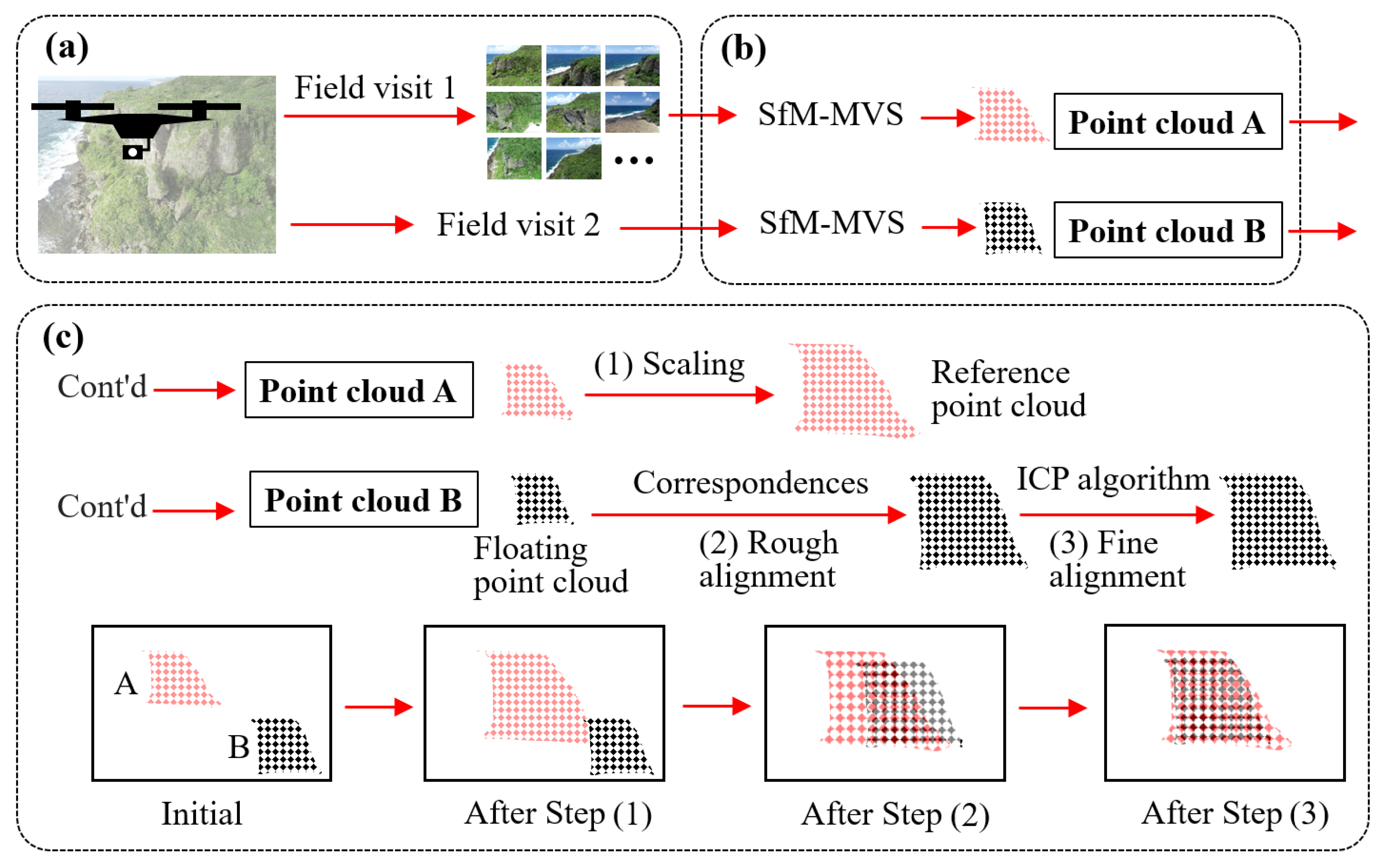
2.1. Image Collection
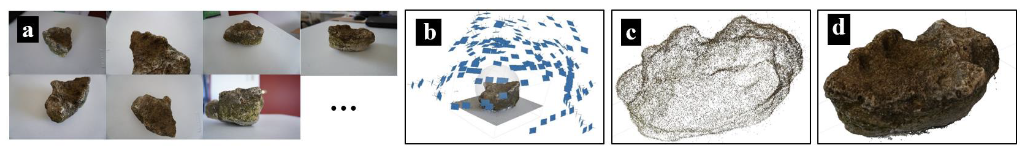
2.2. Point Cloud Reconstruction
2.3. Point Cloud Registration
3. Small-Scale Validation
3.1. Test Configuration
3.2. Point Cloud Reconstruction
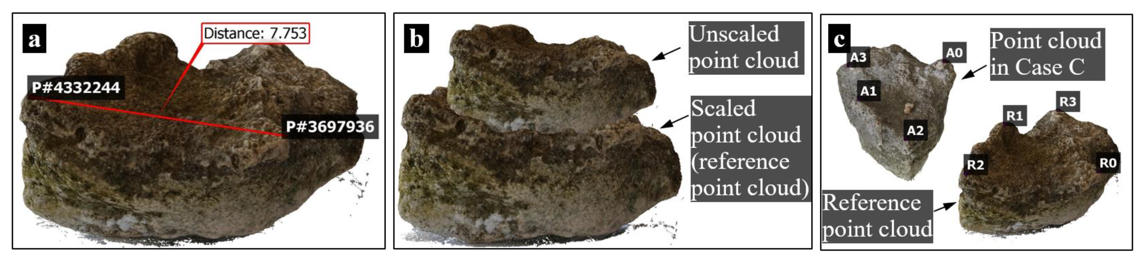
3.3. Point Cloud Registration
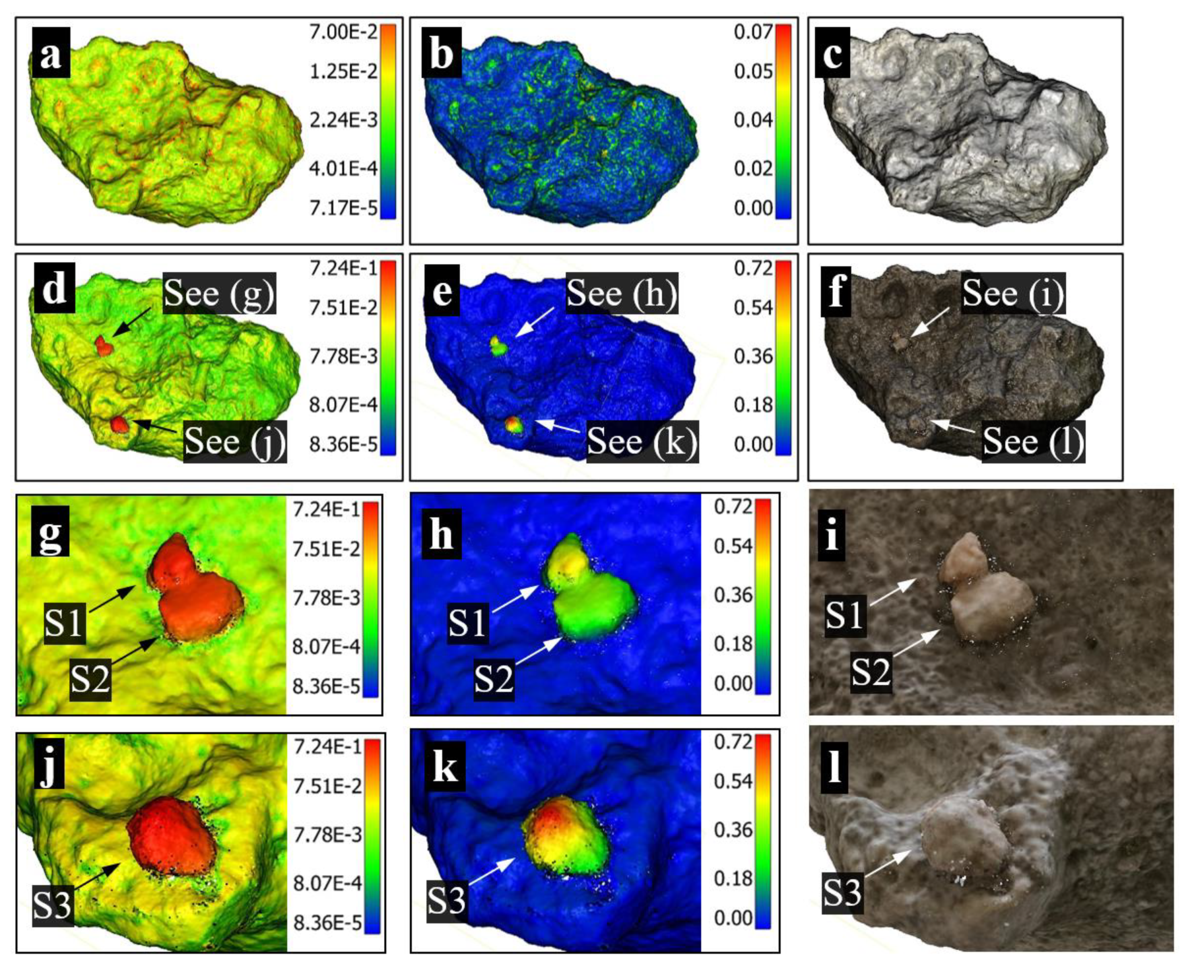
3.4. Point Cloud Comparison
4. Field Validation
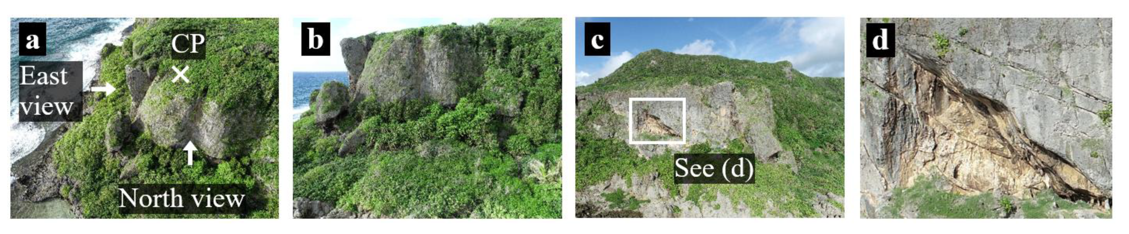
4.1. Site Description
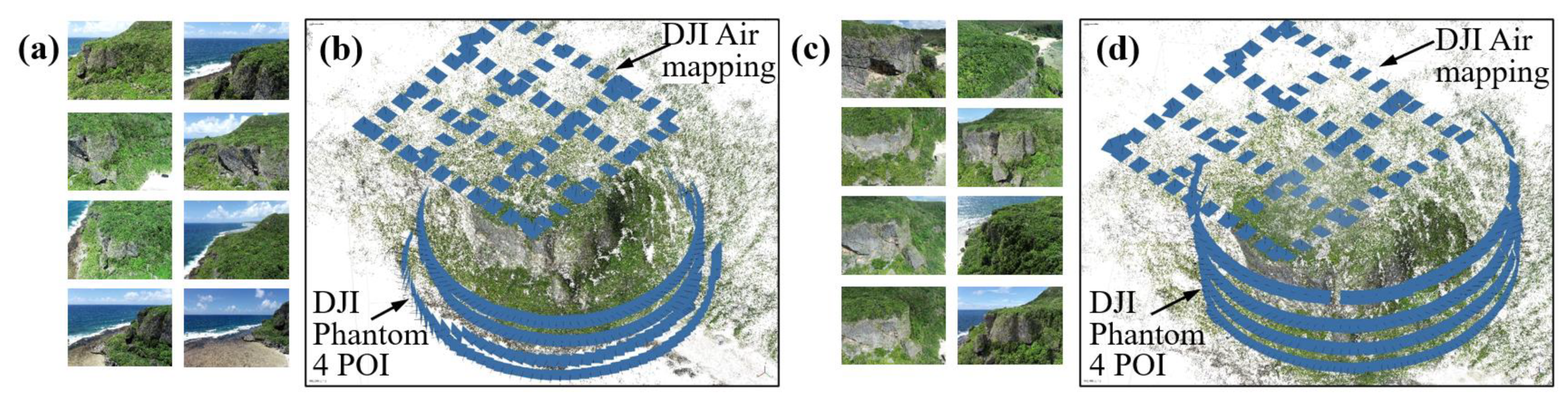
4.2. UAV Operation, Data Collection, and Point Cloud Reconstruction
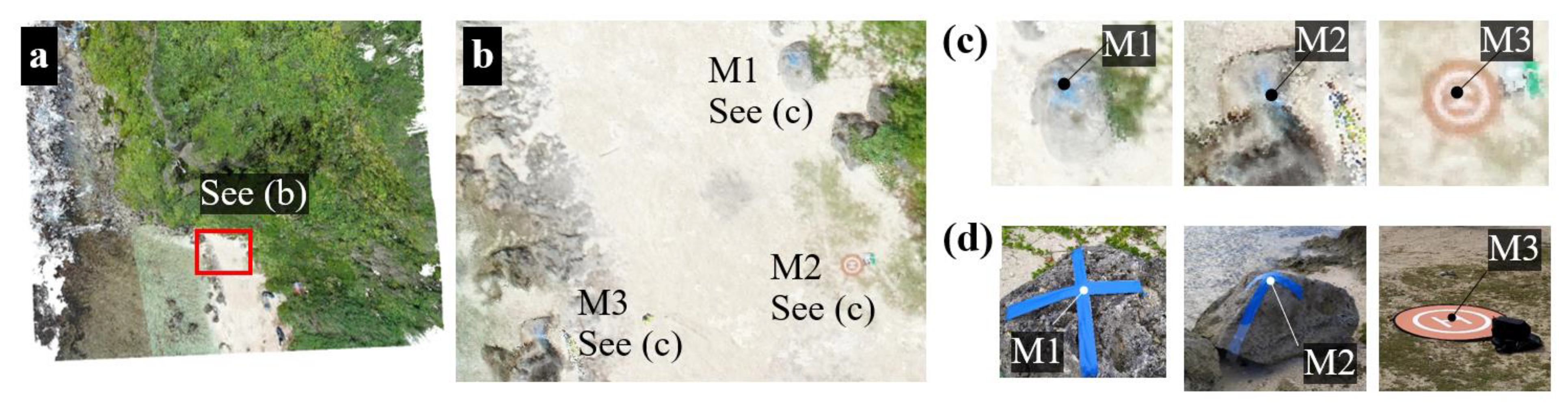
4.3. Point Cloud Registration
4.4. Cliff Monitoring
5. Discussion
6. Conclusions
Funding
Data Availability Statement
Acknowledgments
Conflicts of Interest
References
- Guam Coastal Zone Management Program and Draft Environmental Impact Statement; National Oceanic and Atmospheric Administration, U.S. Department of Commerce: New York, NY, USA, 1979.
- Emery, K.O.; Kuhn, G.G. Sea cliffs: Their processes, profiles, and classification. Geol. Soc. Am. Bull. 1982, 93, 644–654. [Google Scholar] [CrossRef]
- Guam Hazard Mitigation Plan, Guam Homeland Security Office. 2019. Available online: https://ghs.guam.gov/sites/default/files/final_2019_guam_hmp_20190726.pdf (accessed on 7 August 2021).
- Thieler, E.R.; Danforth, W.W. Historical shoreline mapping (II): Application of the digital shoreline mapping and analysis systems (DSMS/DSAS) to shoreline change mapping in Puerto Rico. J. Coast. Res. 1994, 10, 600–620. [Google Scholar]
- Sear, D.A.; Bacon, S.R.; Murdock, A.; Doneghan, G.; Baggaley, P.; Serra, C.; LeBas, T.P. Cartographic, geophysical and diver surveys of the medieval town site at Dunwich, Suffolk, England. Int. J. Naut. Archaeol. 2011, 40, 113–132. [Google Scholar] [CrossRef]
- Westoby, M.J.; Lim, M.; Hogg, M.; Pound, M.J.; Dunlop, L.; Woodward, J. Cost-effective erosion monitoring of coastal cliffs. Coast. Eng. 2018, 138, 152–164. [Google Scholar] [CrossRef]
- Letortu, P.; Jaud, M.; Grandjean, P.; Ammann, J.; Costa, S.; Maquaire, O.; Delacourt, C. Examining high-resolution survey methods for monitoring cliff erosion at an operational scale. GIScience Remote Sens. 2018, 55, 457–476. [Google Scholar] [CrossRef]
- Rosser, N.J.; Petley, D.N.; Lim, M.; Dunning, S.A.; Allison, R.J. Terrestrial laser scanning for monitoring the process of hard rock coastal cliff erosion. Q. J. Eng. Geol. Hydrogeol. 2005, 38, 363–375. [Google Scholar] [CrossRef]
- Hayakawa, Y.S.; Obanawa, H. Volumetric Change Detection in Bedrock Coastal Cliffs Using Terrestrial Laser Scanning and UAS-Based SfM. Sensors 2020, 20, 3403. [Google Scholar] [CrossRef]
- Klemas, V.V. Coastal and environmental remote sensing from unmanned aerial vehicles: An overview. J. Coast. Res. 2015, 31, 1260–1267. [Google Scholar] [CrossRef] [Green Version]
- Crommelinck, S.; Bennett, R.; Gerke, M.; Nex, F.; Yang, M.Y.; Vosselman, G. Review of automatic feature extraction from high-resolution optical sensor data for UAV-based cadastral mapping. Remote Sens. 2016, 8, 689. [Google Scholar] [CrossRef] [Green Version]
- Nex, F.; Remondino, F. UAV for 3D mapping applications: A review. Appl. Geomat. 2014, 6, 1–15. [Google Scholar] [CrossRef]
- Duffy, J.P.; Shutler, J.D.; Witt, M.J.; DeBell, L.; Anderson, K. Tracking fine-scale structural changes in coastal dune morphology using kite aerial photography and uncertainty-assessed structure-from-motion photogrammetry. Remote Sens. 2018, 10, 1494. [Google Scholar] [CrossRef] [Green Version]
- Fonstad, M.A.; Dietrich, J.T.; Courville, B.C.; Jensen, J.L.; Carbonneau, P.E. Topographic structure from motion: A new development in photogrammetric measurement. Earth Surf. Process. Landf. 2013, 38, 421–430. [Google Scholar] [CrossRef] [Green Version]
- Jaud, M.; Bertin, S.; Beauverger, M.; Augereau, E.; Delacourt, C. RTK GNSS-Assisted Terrestrial SfM Photogrammetry without GCP: Application to Coastal Morphodynamics Monitoring. Remote Sens. 2020, 12, 1889. [Google Scholar] [CrossRef]
- Forlani, G.; Pinto, L.; Roncella, R.; Pagliari, D. Terrestrial photogrammetry without ground control points. Earth Sci. Inform. 2014, 7, 71–81. [Google Scholar] [CrossRef]
- Chiang, K.W.; Tsai, M.L.; Chu, C.H. The development of an UAV borne direct georeferenced photogrammetric platform for ground control point free applications. Sensors 2012, 12, 9161–9180. [Google Scholar] [CrossRef] [PubMed] [Green Version]
- Turner, D.; Lucieer, A.; Wallace, L. Direct georeferencing of ultrahigh-resolution UAV imagery. IEEE Trans. Geosci. Remote Sens. 2013, 52, 2738–2745. [Google Scholar] [CrossRef]
- Taddia, Y.; Stecchi, F.; Pellegrinelli, A. Coastal Mapping using DJI Phantom 4 RTK in Post-Processing Kinematic Mode. Drones 2020, 4, 9. [Google Scholar] [CrossRef] [Green Version]
- Peppa, M.V.; Hall, J.; Goodyear, J.; Mills, J.P. Photogrammetric assessment and comparison of DJI Phantom 4 pro and phantom 4 RTK small unmanned aircraft systems. ISPRS Geospat. Week 2019, XLII-2/W13, 503–509. [Google Scholar] [CrossRef] [Green Version]
- Urban, R.; Reindl, T.; Brouček, J. Testing of drone DJI Phantom 4 RTK accuracy. In Advances and Trends in Geodesy, Cartography and Geoinformatics II. In Proceedings of the 11th International Scientific and Professional Conference on Geodesy, Cartography and Geoinformatics (GCG 2019), Demänovská Dolina, Low Tatras, Slovakia, 10–13 September 2019; CRC Press: Boca Raton, FA, USA; p. 99. [Google Scholar]
- Chen, Y.; Medioni, G. Object modelling by registration of multiple range images. Image Vis. Comput. 1992, 10, 145–155. [Google Scholar] [CrossRef]
- Besl, P.J.; McKay, N.D. Method for registration of 3-D shapes. In Sensor Fusion IV: Control Paradigms and Data Structures; International Society for Optics and Photonics: Washington, DC, USA, 1992; Volume 1611, pp. 586–606. [Google Scholar]
- Costantino, D.; Settembrini, F.; Pepe, M.; Alfio, V.S. Develop of New Tools for 4D Monitoring: Case Study of Cliff in Apulia Region (Italy). Remote Sens. 2021, 13, 1857. [Google Scholar] [CrossRef]
- Obanawa, H.; Hayakawa, Y.S. Variations in volumetric erosion rates of bedrock cliffs on a small inaccessible coastal island determined using measurements by an unmanned aerial vehicle with structure-from-motion and terrestrial laser scanning. Prog. Earth Planet. Sci. 2018, 5, 1–10. [Google Scholar] [CrossRef] [Green Version]
- Michoud, C.; Carrea, D.; Costa, S.; Derron, M.H.; Jaboyedoff, M.; Delacourt, C.; Davidson, R. Landslide detection and monitoring capability of boat-based mobile laser scanning along Dieppe coastal cliffs, Normandy. Landslides 2015, 12, 403–418. [Google Scholar] [CrossRef]
- Dewez, T.J.B.; Leroux, J.; Morelli, S. Cliff Collapse Hazard from Repeated Multicopter UAV Acquisitions: Return on Experience. International Archives of the Photogrammetry. Remote Sens. Spat. Inf. Sci. 2016, 41, 805–811. [Google Scholar] [CrossRef] [Green Version]
- Stumpf, A.; Malet, J.P.; Allemand, P.; Pierrot-Deseilligny, M.; Skupinski, G. Ground-based multi-view photogrammetry for the monitoring of landslide deformation and erosion. Geomorphology 2015, 231, 130–145. [Google Scholar]
- Long, N.; Millescamps, B.; Pouget, F.; Dumon, A.; Lachaussee, N.; Bertin, X. Accuracy assessment of coastal topography derived from UAV images. The International Archives of Photogrammetry. Remote Sens. Spat. Inf. Sci. 2016, 41, 1127. [Google Scholar]
- Chaiyasarn, K.; Kim, T.K.; Viola, F.; Cipolla, R.; Soga, K. Distortion-free image mosaicing for tunnel inspection based on robust cylindrical surface estimation through structure from motion. J. Comput. Civ. Eng. 2016, 30, 04015045. [Google Scholar] [CrossRef]
- Dietrich, J.T. Bathymetric structure--from--motion: Extracting shallow stream bathymetry from multi--view stereo photogrammetry. Earth Surf. Process. Landf. 2017, 42, 355–364. [Google Scholar] [CrossRef]
- Bhadrakom, B.; Chaiyasarn, K. As-built 3D modeling based on structure from motion for deformation assessment of historical buildings. Int. J. Geomate 2016, 11, 2378–2384. [Google Scholar] [CrossRef]
- Lowe, D.G. Distinctive image features from scale-invariant keypoints. Int. J. Comput. Vis. 2004, 60, 91–110. [Google Scholar] [CrossRef]
- Shi, J. Good features to track. In Proceedings of the Computer Vision and Pattern Recognition, Proceedings CVPR’94, IEEE Computer Society Conference on IEEE, Seattle, WA, USA, 21–23 June 1994; pp. 593–600. [Google Scholar]
- Rosten, E.; Drummond, T. Fusing points and lines for high performance tracking. In Proceedings of the Tenth IEEE International Conference on Computer Vision (ICCV’05), Beijing, China, 17–21 October 2005; Volumes 1–2, pp. 1508–1515. [Google Scholar]
- Harris, C.; Stephens, M. A combined corner and edge detector. Alvey Vis. Conf. 1988, 15, 50. [Google Scholar]
- Leutenegger, S.; Chli, M.; Siegwart, R.Y. BRISK: Binary robust invariant scalable keypoints. In Proceedings of the 2011 International Conference on Computer Vision, Barcelona, Spain, 6–13 November 2011; pp. 2548–2555. [Google Scholar]
- Bay, H.; Tuytelaars, T.; Van Gool, L. Surf: Speeded up robust features. In European Conference on Computer Vision; Springer: Berlin/Heidelberg, Germany, 2006; pp. 404–417. [Google Scholar]
- James, M.R.; Robson, S. Straightforward reconstruction of 3D surfaces and topography with a camera: Accuracy and geoscience application. J. Geophys. Res. Earth Surf. 2012, 117, F03017. [Google Scholar] [CrossRef] [Green Version]
- Furukawa, Y.; Hernández, C. Multi-view stereo: A tutorial. Found. Trends Comput. Graph. Vis. 2015, 9, 1–148. [Google Scholar] [CrossRef] [Green Version]
- Smith, M.W.; Carrivick, J.L.; Quincey, D.J. Structure from motion photogrammetry in physical geography. Prog. Phys. Geogr. 2016, 40, 247–275. [Google Scholar] [CrossRef] [Green Version]
- AgiSoft Metashape Professional (Version 1.6.2) (Software). 2020. Available online: http://www.agisoft.com/downloads/installer/ (accessed on 1 April 2020).
- CloudCompare (version 2.10.2) [GPL Software]. 2020. Available online: http://www.cloudcompare.org/ (accessed on 1 June 2020).
- Pix4Dcapture (Version 4.10.0) (Smartphone app). 2020. Available online: https://www.pix4d.com/product/pix4dcapture (accessed on 1 June 2020).
- DJI GO 4 (Version 4.3.36) (Smartphone app). 2020. Available online: https://www.dji.com/downloads/djiapp/dji-go-4 (accessed on 1 June 2020).
- Grottoli, E.; Biausque, M.; Rogers, D.; Jackson, D.W.; Cooper, J.A.G. Structure-from-Motion-Derived Digital Surface Models from Historical Aerial Photographs: A New 3D Application for Coastal Dune Monitoring. Remote Sens. 2021, 13, 95. [Google Scholar] [CrossRef]


| Test Case | Surface Texture | Lighting Condition | Geometric Change | Sample and Test Environment |
|---|---|---|---|---|
| Case A | Dark | Indoor lighting condition; daylight was the only light source | Reference dataset | 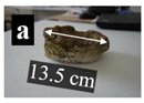 |
| Case B | Light | Outdoor lighting condition; the sample was directly under sunlight | No geometric change was made | 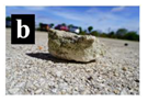 |
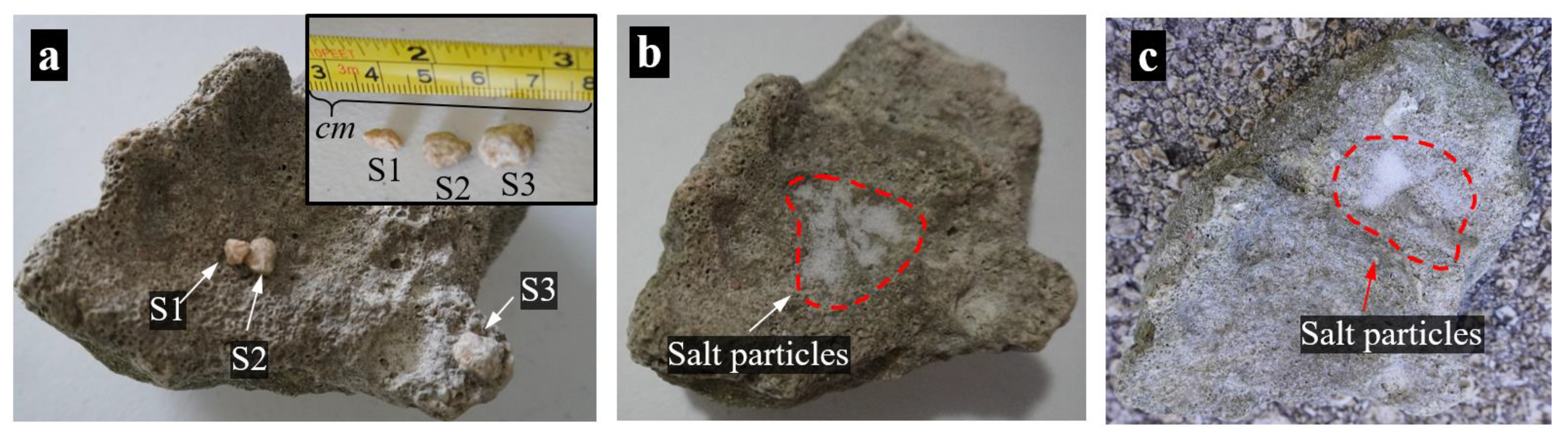
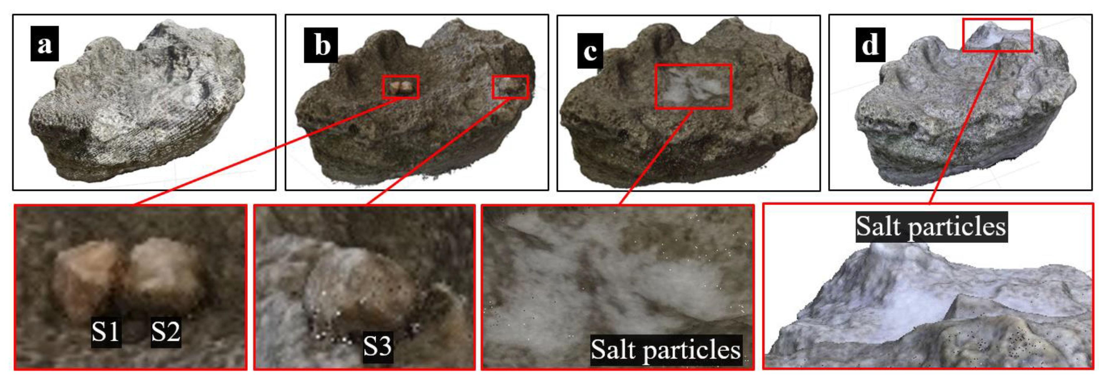
| Case C | Light | Indoor lighting condition; daylight was the only light source | Three small stones were added (see Figure 2a) |  |
| Case D | Light | Indoor lighting condition; the roof lamp was the only light source | A thin layer of salt particles was added (see Figure 2b) | 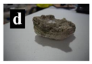 |
| Case E | Light | Outdoor lighting condition; the sample was placed in the shadow | A thin layer of salt particles was added to a different location (see Figure 2c) | 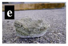 |
| Marker Distance | Field Measurement | CloudCompare Measurement | Scaling Factor Calculation | |
|---|---|---|---|---|
| M1 to M2 | 17.48 m | 16.61 | 1.052 m/1 | Average: 1.054 m/1 |
| M1 to M3 | 10.06 m | 9.52 | 1.057 m/1 | |
| M 2 to M3 | 14.99 m | 14.22 | 1.054 m/1 | |
Publisher’s Note: MDPI stays neutral with regard to jurisdictional claims in published maps and institutional affiliations. |
© 2021 by the author. Licensee MDPI, Basel, Switzerland. This article is an open access article distributed under the terms and conditions of the Creative Commons Attribution (CC BY) license (https://creativecommons.org/licenses/by/4.0/).
Share and Cite
Kong, X. Identifying Geomorphological Changes of Coastal Cliffs through Point Cloud Registration from UAV Images. Remote Sens. 2021, 13, 3152. https://doi.org/10.3390/rs13163152
Kong X. Identifying Geomorphological Changes of Coastal Cliffs through Point Cloud Registration from UAV Images. Remote Sensing. 2021; 13(16):3152. https://doi.org/10.3390/rs13163152
Chicago/Turabian StyleKong, Xiangxiong. 2021. "Identifying Geomorphological Changes of Coastal Cliffs through Point Cloud Registration from UAV Images" Remote Sensing 13, no. 16: 3152. https://doi.org/10.3390/rs13163152
APA StyleKong, X. (2021). Identifying Geomorphological Changes of Coastal Cliffs through Point Cloud Registration from UAV Images. Remote Sensing, 13(16), 3152. https://doi.org/10.3390/rs13163152