Abstract
Polarimetric synthetic aperture radar (PolSAR) image classification is one of the basic methods of PolSAR image interpretation. Deep learning algorithms, especially convolutional neural networks (CNNs), have been widely used in PolSAR image classification due to their powerful feature learning capabilities. However, a single neuron in the CNN cannot represent multiple polarimetric attributes of the land cover. The capsule network (CapsNet) uses vectors instead of the single neuron to characterize the polarimetric attributes, which improves the classification performance compared with traditional CNNs. In this paper, a hierarchical capsule network (HCapsNet) is proposed for the land cover classification of PolSAR images, which can consider the deep features obtained at different network levels in the classification. Moreover, we adopt three attributes to uniformly describe the scattering mechanisms of different land covers: phase, amplitude, and polarimetric decomposition parameters, which improves the generalization performance of HCapsNet. Furthermore, conditional random field (CRF) is added to the classification framework to eliminate small isolated regions of the intra-class. Comprehensive evaluations are performed on three PolSAR datasets acquired by different sensors, which demonstrate that our proposed method outperforms other state-of-the-art methods.
1. Introduction
Polarimetric synthetic aperture radar (PolSAR) can provide unique and useful information under all-weather and multi-climate conditions, and has been widely used in vegetation distribution [1], disaster assessment [2], ocean research [3], and other fields. Due to its advantages in obtaining full-polarization information, PolSAR image land cover classification has received increasingly more attention in recent years and has become crucial for PolSAR image interpretation.
To date, many PolSAR image classification methods have been proposed. The earliest classification method was designed based on the statistical characteristics of PolSAR data, such as the Wishart distribution [4], spherically invariant random vector [5], and so on. However, these methods rely heavily on the accuracy of the statistical model. Moreover, the parameter estimation of the statistical models is complicated and sensitive to the PolSAR data acquired by different sensors and platforms. Therefore, these methods often fail to obtain satisfactory classification results with different PolSAR datasets.
With the development of machine learning, many classic classification algorithms have emerged for PolSAR image classification, such as support vector machine (SVM) [6], decision tree (DT) [7], Markov random field (MRF) [8], and so on. These traditional machine learning algorithms are easy to use and suitable for different datasets. However, these methods rely heavily on the extracted classification features, which are not robust to different PolSAR datasets. Due to the limitation of capabilities in feature representation and deep feature extraction, satisfactory classification results cannot be easily obtained when dealing with the classification for the PolSAR data with polarimetric scattering ambiguity.
Benefiting from the emergence of deep learning algorithms, the shortcomings of traditional machine learning algorithms in feature representation and deep feature extraction can be solved. In recent years, a series of deep learning algorithms made remarkable achievements in the field of PolSAR image classification [9,10]. Chen et al. [11] established a polarimetric feature-driven deep CNN classification scheme for PolSAR image land cover classification. Li et al. [12] proposed a sliding window fully convolutional network with sparse coding for PolSAR image classification. Xie et al. [13] proposed a deep learning network combining recurrent complex-valued CNN and a Wishart classifier, and achieved competitive classification results. However, CNNs still have some shortcomings in PolSAR image land cover classification. The most common deficiency is the poor small sample performance, i.e., the classification accuracy based on CNNs is generally low with a small training sample size. Due to the complex polarimetric backscattering of different land covers, the same class may have different scattering mechanisms or the same polarimetric scattering mechanism can represent different land covers [14,15,16,17,18,19]. In the network structure of CNNs, an active neuron can only represent one entity, and the unicity of its dimension determines that the neuron itself cannot represent multiple attributes of the same entity simultaneously. Therefore, in the PolSAR image classification based on CNNs, a class may have more than one scattering mechanisms. The relationship of these scattering mechanisms can only hide into a lot of network parameters, which requires enough training samples to update network parameters, resulting in that the adjustment of the parameters is tedious and time-consuming. In addition, sample imbalance may also cause underfitting or overfitting of CNN model training. Therefore, in the case of small sample training and sample imbalance, the CNN cannot train an accurate classification model.
In recent years, the capsule network (CapsNet) has been applied to many image applications and it has obtained more competitive results than CNNs [20,21,22]. Sabour and Hinton et al. [23] proposed the CapsNet, which encapsulates multiple neurons into a vector. CapsNet uses the length of the capsule to represent the probability that the entity exists and uses the direction of the capsule to represent the instantiation parameters, which breaks the limitation that an active neuron in traditional CNNs can only represent one entity [24]. Guo et al. [25] used an improved capsule network for SAR target recognition, which indicates that the capsule network has good robustness in terms of recognition accuracy, convergence, image changes, and viewpoint changes. Phaye et al. [26] proposed frameworks customizing the CapsNet by replacing the standard convolutional layers with densely connected convolutions, which essentially adds a deeper convolutional network. Wang et al. [27] combined CapsNet and residual network (ResNet) to improve the classification accuracy of LiDAR data. As PolSAR images contain complex backscattering information, which is more difficult to interpret than optical and hyperspectral images, only a few studies have used CapsNet in PolSAR images. Zhang et al. [28] used the CNN as CapsNet’s feature extractor for PolSAR image scene classification, which enhances the CapsNet’s ability to extract deep features. Until now, it has not been discovered that researchers have used CapsNet in land cover classification of PolSAR images. One of the problems that make PolSAR image classification difficult is that the same land cover may have different scattering mechanisms, and the same scattering mechanism may represent different land covers. CapsNet can jointly represent multiple attributes of objects, which is useful for representing multiple scattering mechanisms of land covers. In this paper, we will explore the potential ability of CapsNet in PolSAR image land cover classification and make some contributions in network structure and parameter settings based on the characteristics of PolSAR data.
The typical CapsNet uses a single convolutional layer in the feature extraction stage, which is insufficient in deep feature extraction. To overcome this problem, many studies replace a single convolutional layer with a deeper convolutional network [29,30,31]. However, in the land cover classification of PolSAR images, the deeper network will bring two problems: one is that when the number of training samples is poor, the model is difficult to train and easy to overfit. The other is that the loss backpropagation distance increases, which is not conducive to weight update. In the deep learning network, with the deepening of the network depth, the problem of gradient disappearance will become increasingly more obvious. In addition, the deep features contain more discriminative information than raw features, but the detailed information contained in the raw features is lost. As stated before, one land cover may have multiple scattering mechanisms, and multiple land covers may also exhibit the same scattering mechanism. Thus, sample labeling is difficult for PolSAR images and the number of training samples is often small, which is not conducive for the training of deep CNN [32]. How to achieve the extraction of deep features and simultaneously shorten the backpropagation distance in CapsNet has become a challenging problem.
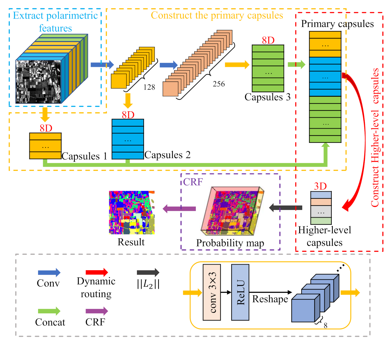
In this paper, we propose an improved capsule network structure, called the hierarchical capsule network (HCapsNet) for PolSAR image classification, as shown in Figure 1. HCapsNet uses two convolutional layers to extract deep information from polarimetric features. The primary capsules are composed of deep features obtained at different network levels. Therefore, the primary capsules contain shallow and deep features. The capsules of each layer are connected to the higher-level capsules through dynamic routing, which means that the backpropagation of the loss can directly reach the capsules of each layer instead of backpropagating layer by layer. A shorter backpropagation distance can make the gradient transmission more efficient and the network converges faster. Therefore, rich deep features and short backpropagation distance enable the proposed method to learn more useful features from the small-size training samples. In addition, the authors of [27] pointed out that the higher-level capsule represents more complex entities and should have more degrees of freedom than the lower-level capsule. The dimension of the higher-level capsule represents the number of entity attributes. However, in PolSAR data, due to the complexity of polarimetric scattering mechanisms, the number of scattering mechanisms included in different land covers is uncertain. Therefore, we divide the polarimetric features into three discriminative attributes, i.e., phase, amplitude, and polarimetric decomposition, which are used to uniformly describe the scattering mechanism of land covers with different sensors, bands, and resolutions. For example, the main scattering mechanism of forest areas and potato areas is volume scattering. It is difficult to distinguish forest and potato accurately only by relying on the features of volume scattering, but the amplitude of the forest is higher than potato. Due to the refraction of the double-bounce scattering path, the phase difference with the co-polarization is close to , so the building areas have a higher phase difference than other areas. Polarimetric decomposition parameters can divide the feature space into 16 regions, and each region corresponds to a scattering mechanism, so they can also be used as a general attribute to describe the scattering mechanism of land covers. Based on the number of polarimetric feature attributes, we attempt to reduce the dimension of the higher-level capsule, thereby intuitively reducing the number of parameters in the dynamic routing process.
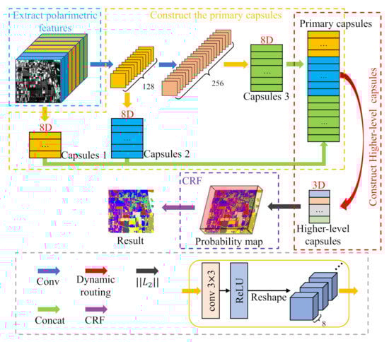
Figure 1.
The architecture of the proposed classification method.
In the field of image classification, the conditional random field (CRF) [33,34], as a postprocessing technique, has been widely used in combination with many classification methods [35]. Wang et al. [36] used a CNN combined with the CRF to extract the spatial distribution of winter wheat from remote sensing images. Zhang et al. [37] used the probability result obtained by the SVM as the potential energy term of the CRF. We combine the proposed HCapsNet with the CRF to construct a land cover classification framework for PolSAR images, as shown in Figure 1. In this framework, the HCapsNet and the CRF are used to describe the polarimetric information and spatial information of PolSAR images, respectively, to reduce the misclassification of class boundaries and intra-class, respectively. Furthermore, we test the generalization performance of our proposed method. We attempt to use the model trained on the AIRSAR dataset to classify on the RADARSAT-2 dataset. As the proposed method can uniformly and accurately describe scattering mechanisms of land covers, it shows a certain generalization performance in different sensor data. The experimental results on three PolSAR datasets show that the proposed method achieves a better classification results compared with state-of-the-art methods.
The main contributions of the paper are briefly summarized as follows.
- (1)
- The HCapsNet is proposed for land cover classification of PolSAR images. It can simultaneously consider the deep features obtained at different network levels, which describes the polarimetric scattering information of land covers more comprehensively with small training sample size, and significantly reduces the misclassification of class boundaries.
- (2)
- The CRF is combined with the HCapsNet to further refine the classification results. The intra-class misclassifications can be reduced by the spatial information constraints of the CRF.
- (3)
- We adopt three discriminative attributes for land covers of PolSAR data, i.e., phase, amplitude, and polarimetric decomposition, to uniformly describe the scattering mechanism of land covers with different sensors, bands, and resolutions. Moreover, the generalization performance of the proposed method is verified to be better than other comparison methods.
The rest of this paper is organized as follows. In Section 2, the proposed method is introduced, including polarimetric features extraction, primary capsule layer construction, higher-level capsule layer construction, and the CRF. Section 3 lists the experimental results of our proposed method on two AIRSAR and one GF-3 PolSAR datasets as well as the comparisons with other state-of-the-art methods. Evaluations of different method in convergence speed, small sample performance, and extracted discriminative features are also performed. Section 4 gives the discussion of different polarimetric features, different structures, and generalization performance. Finally, conclusions are given in Section 5.
2. Methodology
Figure 1 shows a schematic diagram of the proposed method. The proposed method consists of 4 parts: polarization feature extraction, primary capsule layer construction, higher-level capsule layer construction, and the CRF model optimization. First, the polarimetric features are extracted and constructed into a feature vector. Second, deep features are extracted from the original polarimetric features through two convolutional layers. Moreover, the primary capsules are composed of deep features at different network levels. Then, the primary capsules are connected to the higher-level capsules through dynamic routing. Finally, the probability map of the classification result is calculated and input into the CRF model to further optimize the classification result.
2.1. Polarimetric Feature Extraction
In the full polarization observation, the scattering matrix represents all the information of the target scattering characteristics, the backscattering matrix is expressed as
in which H and V represent horizontal and vertical polarization, respectively. Each element is called the scattering amplitude, which represents the complex backscattering coefficient of the target when it is transmitted in Y polarization and received in X polarization.
In the case of satisfying the reciprocity theorem, the covariance matrix and coherence matrix of the target can be defined as follows [38]:
The co-polarization ratio [39] is defined as the ratio of the scattered energy between the co-polarization channels, which can be written as
The cross-polarization ratio [39] is defined as the scattering energy ratio of the cross-polarization channel and the co-polarization channel, which can be written as
Note that the co- and cross-polarization ratios can also be defined with respect to scattered energy in the HH channel.
Cloude and Pottier [40] proposed a method to extract sample mean parameters using a smoothing algorithm with second-order statistics. Three important polarimetric scattering parameters can be extracted from the coherence matrix —Entropy (H), Anisotropy (A), and Scattering angle ()—can be defined as
where represents the eigenvalue of the coherence matrix . is the key parameter to identify the main scattering mechanism. H describes the statistical disorder of different scattering types. As a supplementary parameter, A can improve the ability to distinguish different types of scattering mechanisms.
In this paper, the eight polarimetric features are extracted for the land cover classification, as shown in Table 1. The eight polarimetric features can be divided into three categories, which are phase, amplitude, and polarimetric decomposition. The first one consists of cross-polarization ratio () and co-polarization ratio (), which are widely used for vegetation classification of PolSAR images [41,42]. The second one includes . As the diagonal elements of the , they contain comprehensive amplitude information and can be directly or indirectly used for PolSAR image classification [43,44]. Moreover, the last one consists of Entropy (H), Anisotropy (A), and Scattering angle (), which are commonly used to describe the scattering mechanisms [45]. As the change intervals of these features are of different orders of magnitude, we adopt a normalization operation to map the features to the range of 0 to 1.

Table 1.
The polarimetric feature set.
2.2. Construction of the Primary Capsule Layer
In CNNs, an activated neuron can only represent one entity, which greatly limits the ability of CNNs to represent object attributes. The CapsNet [23] overcomes this shortcoming of CNNs by encapsulating multiple neurons into a neuron capsule (NC). The length of the NC represents the probability of the existence of the entity, and its direction represents the instantiation parameter. Figure 2 shows the difference between classic CNN and CapsNet. In the deep feature extraction stage, the CapsNet still uses a single convolutional layer as the feature extractor. CNNs are widely used in the PolSAR image classification, which can extract discriminative spatial features and achieve excellent classification accuracy [46]. A convolutional operation can be defined as [47]
where is the i-th feature map of the ()-th convolutional layer, is the j-th feature map of the l-th convolutional layer, N is the number of feature maps of the ()-th convolutional layer, denotes the weight matrix (i.e., the convolution kernel) connecting the i-th feature map of the ()-th layer and the j-th feature map of the l-th layer. Moreover, denotes the bias of the j-th feature map of the convolutional layer. denotes the activation function.
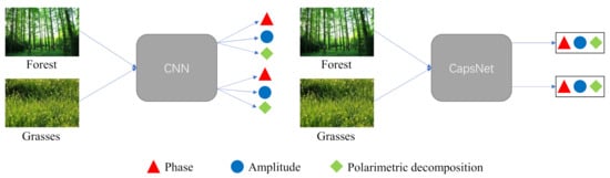
Figure 2.
Illustration of the difference between classic CNN and CapsNet.
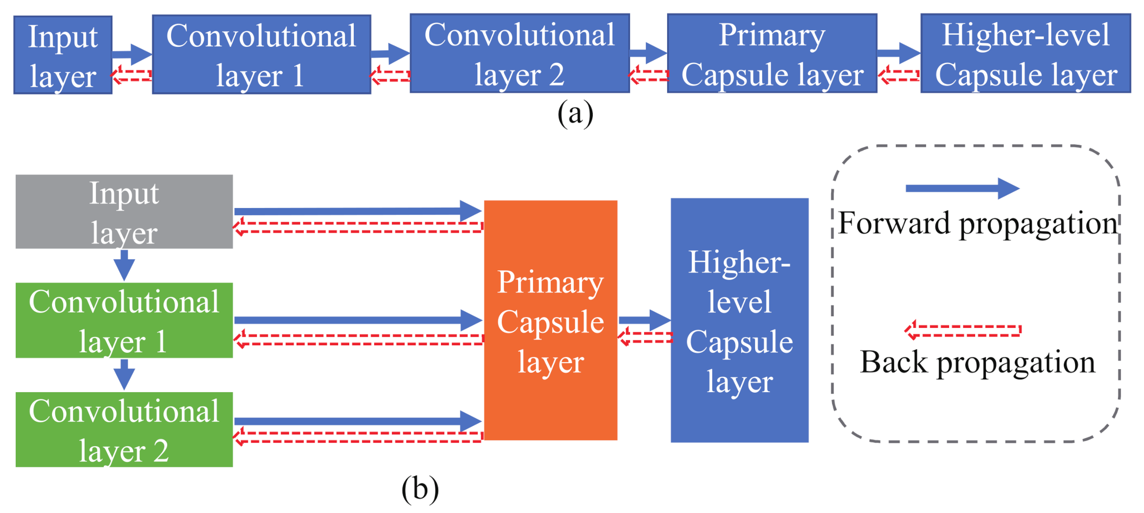
Huang et al. [48] proposed a densely connected convolutional network (DenseNet) to strengthen the feature propagation and encourage the feature reuse. Inspired by this idea, we design a way to construct a primary capsule layer. This design can shorten the distance of backpropagation. As shown in Figure 3b, the backpropagation of the loss can directly reach the capsules of each layer instead of backpropagating layer by layer. The DenseNet connects each layer to every other layer in a feedforward fashion. In our proposed HCapsNet framework, we do not need too deep network levels to extract deep features, and do not encourage deep features to be convolved multiple times. We construct capsules at the input layer and two convolutional layers and use these capsules to construct the primary capsule layer directly.

Figure 3.
Schematic diagram of constructing the primary capsule layer. (a) Traditional method. (b) Proposed method.
The construction process of the primary capsule layer (P) can be defined as
in which represents the output of l-th layer. denotes the “reshape” process, which is used to obtain the capsules () on each layer. As shown in Figure 3a, in traditional methods, the primary capsule layer only has deep features. However, the primary capsule layer constructed by our proposed method can contain both shallow and deep features. Therefore, rich deep features enable the proposed method to describe the object more comprehensively. The short backpropagation distance enables the proposed method to converge faster than traditional methods.
2.3. Construction of the Higher-Level Capsule Layer
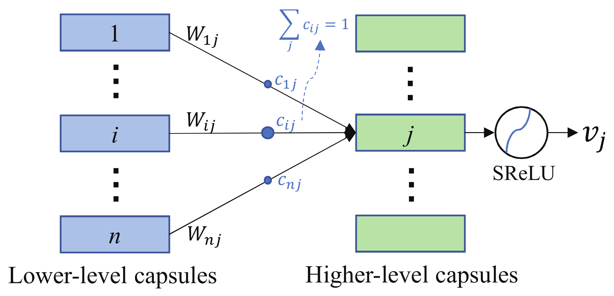
Figure 4 illustrates the dynamic routing process from the lower-level capsule to the higher-level capsule.
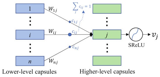
Figure 4.
Connections between the lower-level capsules and higher-level capsules.
The lower-level active capsule is transported to the higher-level capsule using the following formula:
where represents the connection weight matrix from the i-th lower-level capsule to the j-th higher-level capsule. Here, denotes a coupling coefficient that is defined as
where (or ) represents the prior probability from the lower-level capsule i to higher-level capsule j (or k). As the modulus length of the capsule output vector represents the probability of the existence of the entity, a nonlinear squeeze function is needed to compress the modulus length to [0, 1) without changing the direction of the vector. The formula of Squashing Rectified Linear Unit (SReLU) is defined as follows,
In addition, we make a reasonable parameter adjustment based on the characteristics of PolSAR data. Researchers generally consider that higher-level capsules represent more complex entities and should have more dimensions than lower-level capsules [49]. The dimension of higher-level capsules represents the number of polarimetric attributes of the object. However, the polarimetric attributes of land covers depend on categories of the input polarimetric features, such as phase, amplitude and so on. For PolSAR image classification, a polarimetric attribute of land covers can be represented by multiple polarimetric features. The number of polarimetric attributes of land covers is often small. Therefore, higher-level capsules do not require too many dimensions to characterize the polarimetric attributes of land covers. The reduction in the dimensions of the higher-level capsules intuitively reduces the number of network parameters. The connection between the lower-level capsules and the higher-level capsules is shown in Figure 4. N lower-level capsules are connected to M higher-level capsules, and the number of parameters (Num) required is calculated by the following formula:
where and represent the dimension of the lower-level and the higher-level capsule, respectively. At present, most researchers continue to use the parameter settings of the original capsule network, which set to 16 [23,24,25,26,27,28]. This study reduces the size of from 16 to 3, and the number of parameters is reduced by 13/16 times, according to (14).
2.4. Conditional Random Field
The fully connected CRF [34] can consider the spatial context information and realize the correct classification of misclassified pixels through the consideration of local neighborhoods. The energy function of the CRF model consists of the unary potential function and the pairwise potential function. The formula is depicted as follows:
in which represents the unary potential, which is computed independently for each pixel by a classifier. represents the pairwise potential, which is defined as follows:
in which is a label compatibility function. is liner combination weights. and are positions of and . The degrees of nearness and similarity are controlled by the parameter . The smoothness kernel can remove small isolated regions [50]. In the results of PolSAR image classification, intra-class misjudgments are inevitable. Therefore, we use the CRF to eliminate misclassified regions within the class.
2.5. Implementation Details
In detail, the proposed method is shown in Algorithm 1. First, the refined Lee filtering with a window size of 7 × 7 is performed on the PolSAR image. Then, the eight polarimetric features are extracted and constructed into a feature vector. Before training, we initialize the network weights to zero. In the training process, the network weights are iteratively updated and the classifier model can be obtained. We used the margin loss [23] as a loss function of the proposed HCapsNet. The formula of the loss function is depicted as follows:
where , if the true class is k. represents the modulus length of vector , which is the probability that the pixel belongs to class k. and are the lower boundary of the true class and the higher boundary of the false class. The hyperparameter stops the initial learning from shrinking the lengths of the activity vectors of all the higher-level capsules [23].
In the testing process, we use the classifier model to classify the test samples, and obtain the probability map M of the classification results. Finally, the probability map is updated by the CRF, and the pixel-wise class labels can be obtained according to the final probability map.
| Algorithm 1 Proposed method |
|
3. Experiment Results and Analysis
In this section, we evaluate the performance of the proposed method for PolSAR image classification. We first briefly describe the used PolSAR datasets and parameter settings. Afterward, we compare the classification accuracy between the proposed method and other comparison PolSAR image classification methods on three different PolSAR datasets. Finally, under a common comparable framework, we analyze the advantages of the proposed method in terms of convergence speed and small sample performance.
3.1. Data Description and Parameter Settings
In our study, two widely used AIRSAR data and a newly-used GF-3 data are used to validate the effectiveness of the proposed method. All experiments are implemented on the Windows 10 platform, and the basic experimental environment settings are is shown in Table 2.
Table 2.
The basic experimental environment settings.
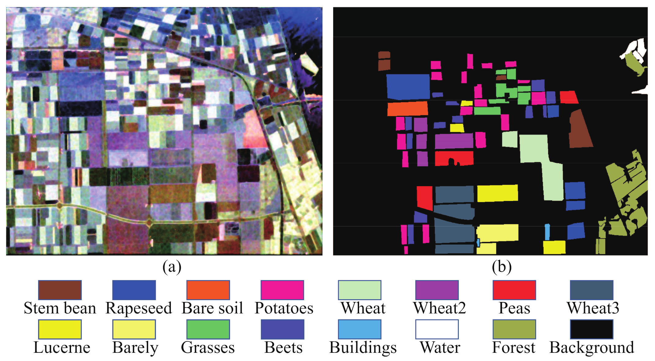
(1) AIRSAR Flevoland dataset: The first quad-polarimetric SAR dataset is the widely used L-band data acquired by the NASA/JPL AIRSAR system over the Flevoland test site in mid-August of 1989. The incidence angle is approximately at the near range and at the far range. Figure 5a is a pseudo-color image formed by PauliRGB decomposition. The size of these data is 750 × 1024. The ground truth data contain 177,018 pixels, including 15 different land cover types, as shown in Figure 5b [13]. One percent of the labeled samples are selected as the training samples. The experimental information is shown in Table 3.
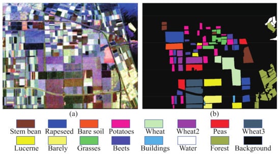
Figure 5.
Flevoland dataset. (a) PauliRGB image (Red: double-bounce scattering power. Green: volume scattering power. Blue: surface scattering power). (b) Ground truth map.
Table 3.
The image information of Flevoland dataset.
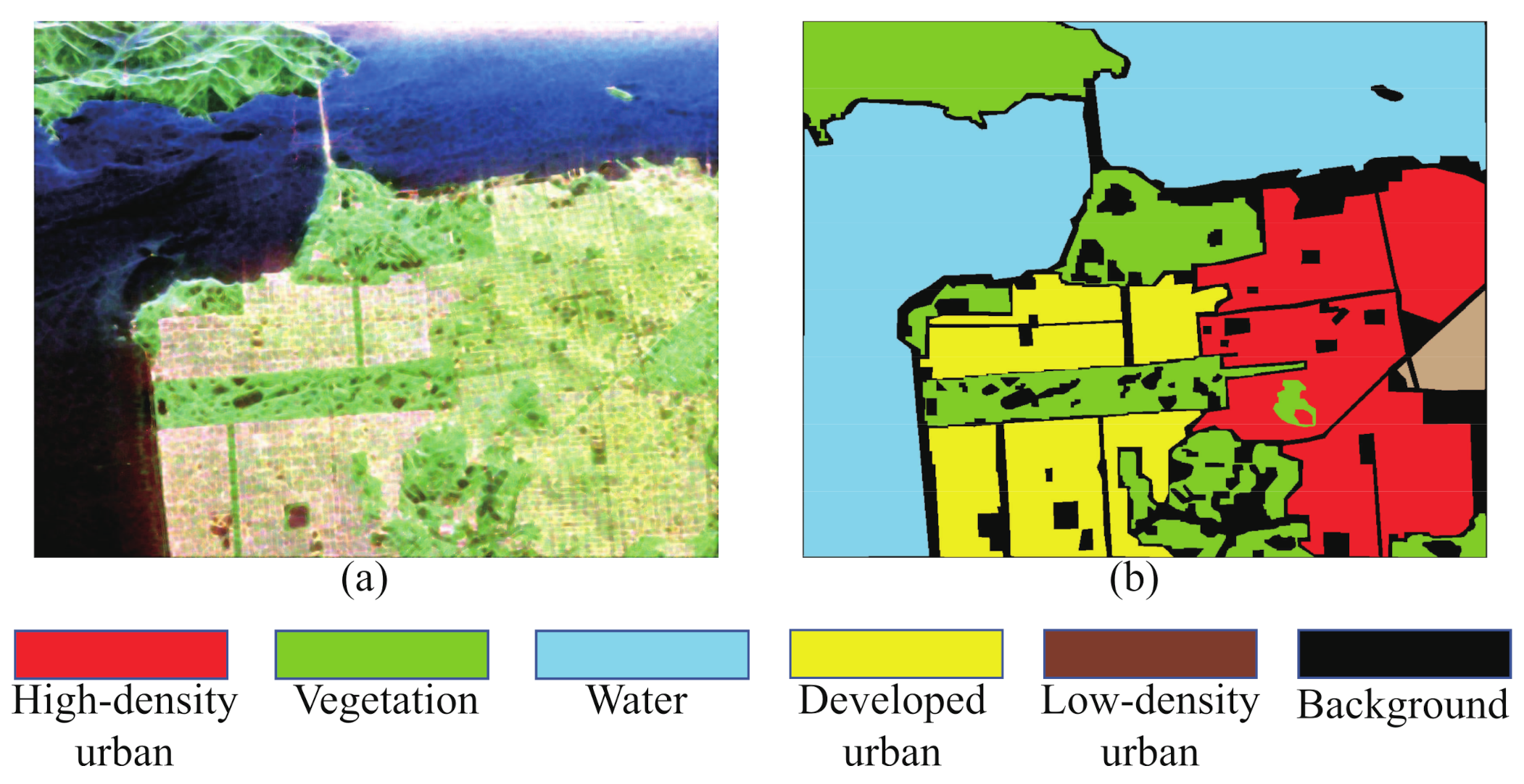
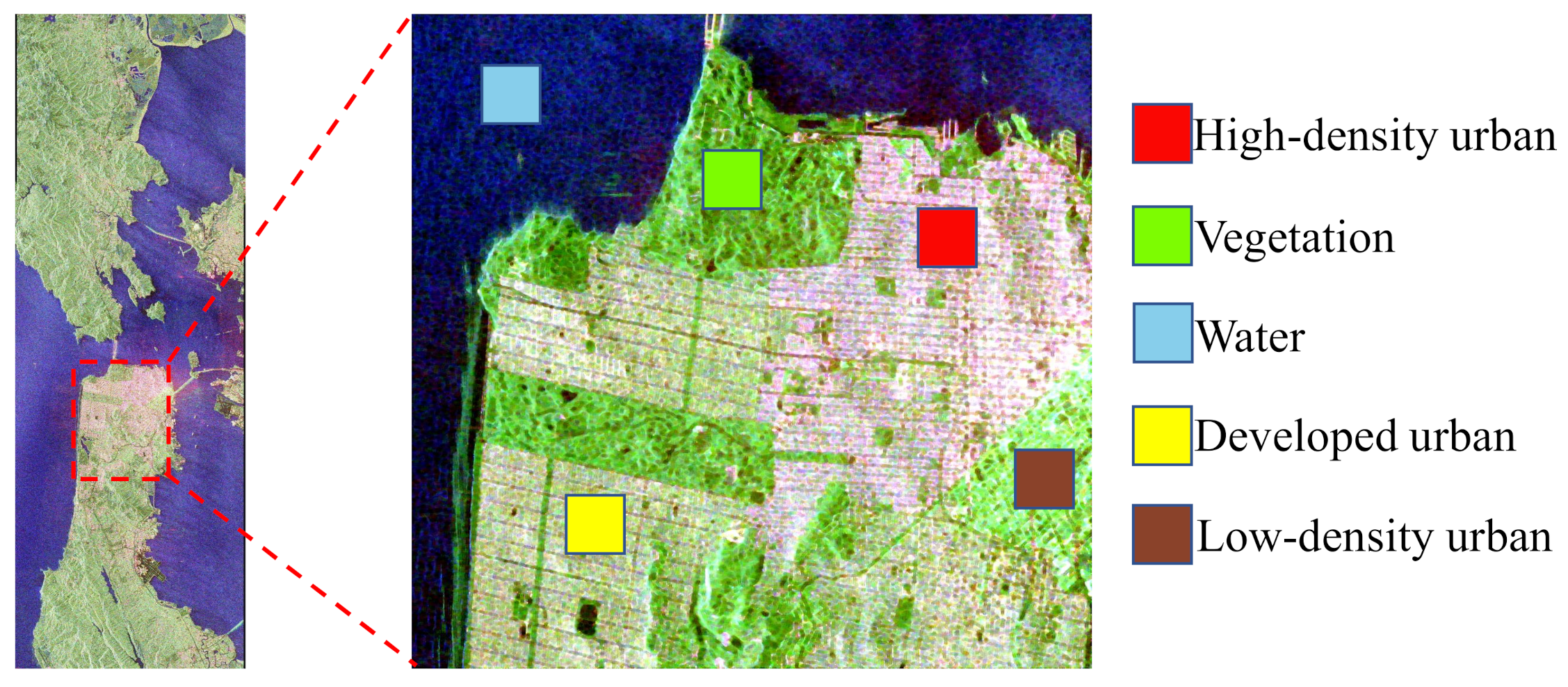
(2) AIRSAR San Francisco dataset: The second quad-polarimetric SAR dataset is also the widely used data acquired by the NASA/JPL AIRSAR system in 1989. The spatial resolution is 10 m. Figure 6a is a pseudo-color image formed by PauliRGB decomposition. The size of these data is 900 × 1024. The ground truth data contain 776,501 pixels, including 5 different land cover types, as shown in Figure 6b [51]; of the labeled samples are selected as the training samples. The experimental information is shown in Table 4.
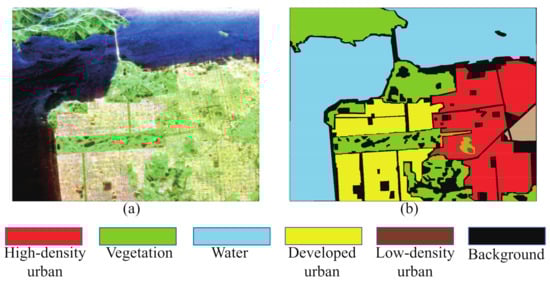
Figure 6.
San Francisco dataset. (a) PauliRGB image (Red: double-bounce scattering power. Green: volume scattering power. Blue: surface scattering power). (b) Ground truth map.
Table 4.
The image information of AIRSAR San Francisco dataset.
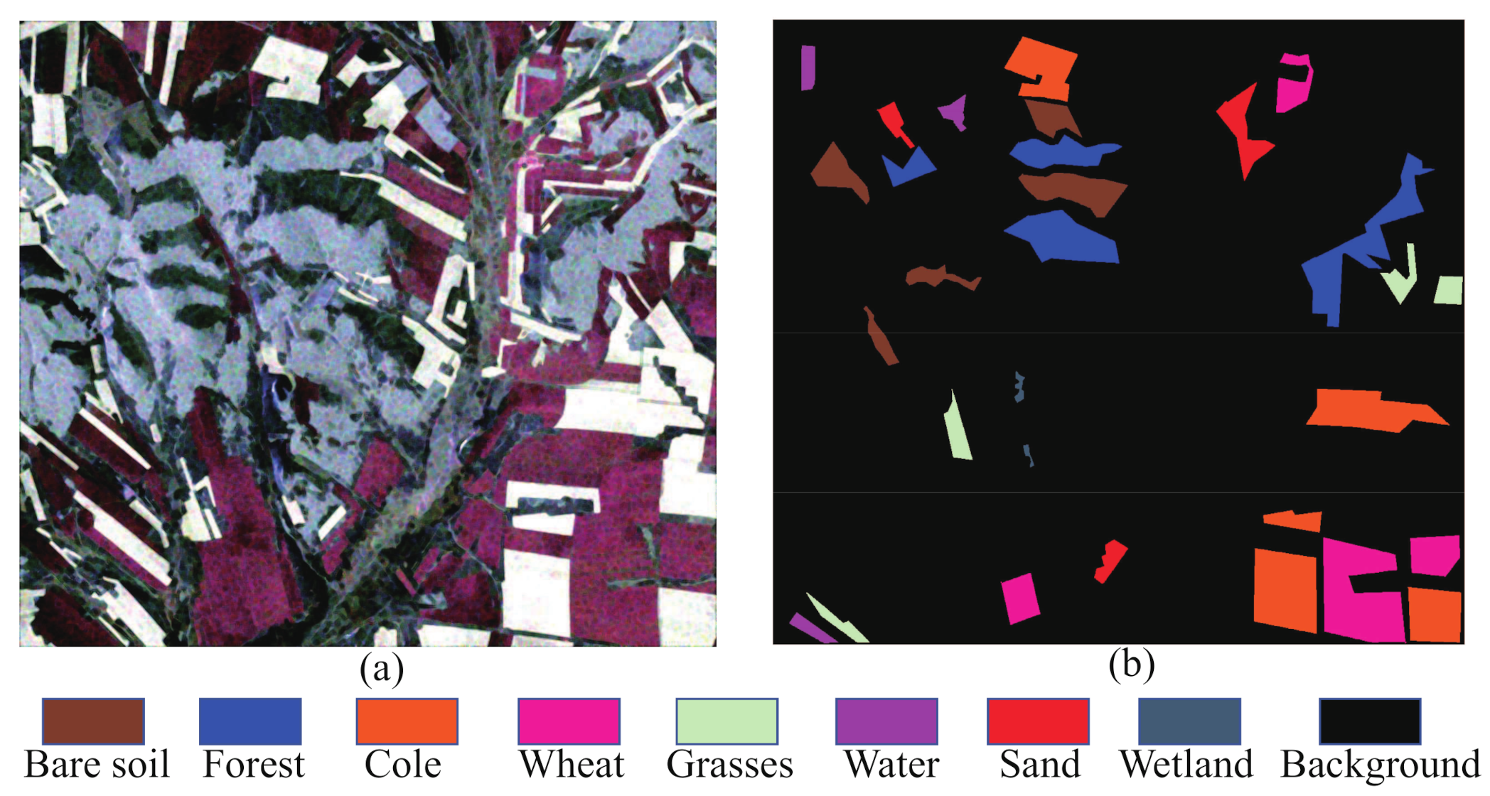
(3) GF-3 Hulunbuir dataset: The third quad-polarimetric SAR dataset is acquired by the GF-3 system in Hulunbuir, China. Figure 7a is a pseudo-color image formed by PauliRGB decomposition. The size is 1147 × 1265 pixels. The ground truth data contain 173,550 pixels, including 8 different land cover types, as shown in Figure 7b; of the labeled samples are selected as the training samples. The experimental information is shown in Table 5.
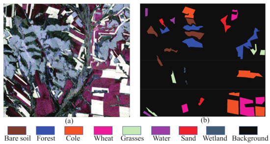
Figure 7.
GF-3 dataset. (a) PauliRGB image (Red: double-bounce scattering power. Green: volume scattering power. Blue: surface scattering power). (b) Ground truth map.
Table 5.
The image information of GF-3 dataset.
We set the network parameters as follows. The size of the patch is 15 × 15 in two AIRSAR data and 9 × 9 in GF-3 data [52]. We use 128 kernels in the first convolutional layer and 256 kernels in the second one, and stride is set as 2. The kernel size is set as 3 × 3. The batch size is set as 16. The “ReLU” is used as the activation function. The dimension of primary capsule is set as 8. This study takes eight commonly used polarimetric features as input, as shown in Table 1, which represents three polarimetric attributes: phase, amplitude, and polarimetric decomposition parameters. Therefore, we set the dimension of the higher-level capsule to 3. Moreover, the “Adam” is employed as an optimizer, and the learning rate is set to 0.001 [53]. The parameters , , and in the loss function are set to 0.9, 0.1, and 0.5 by default [23]. The two hyperparameters in (16), is set to 12, and is set to 3 by default.
3.2. Classification Results of the AIRSAR Flevoland Dataset
To evaluate the performance of the proposed method, other PolSAR image classification methods are employed for performance comparison, including 1D-CNN [54], 2D-CNN [11], DenseNet [32], and CapsNet [23]. CapsNet-3 indicates that the dimension of higher-level capsule is set as 3, while the remaining of the structure and parameters are the same as the CapsNet. For the sake of fair comparison, all methods use the same training samples and test samples. To avoid the negative influence of network instability on the classification, the experiments are repeated five times, and the average value is taken as the final classification result. The classification maps are shown in the Figure 8. Table 6 shows the classification accuracies of each class with different classification methods, as well as the OA, AA, and Kappa of the AIRSAR Flevoland dataset classification results.
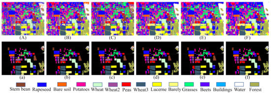
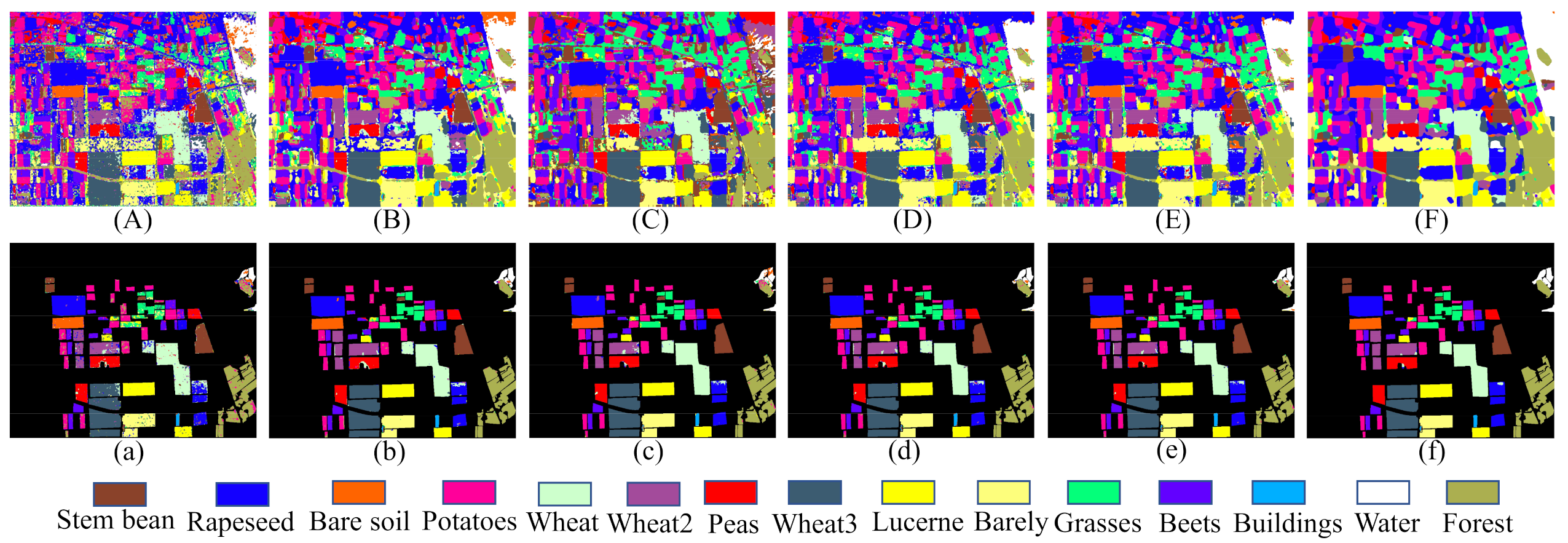
Figure 8.
Classification maps of the AIRSAR Flevoland dataset. (A) 1D-CNN. (B) 2D-CNN. (C) DenseNet. (D) CapsNet. (E) CapsNet-3. (F) Proposed method. (a–f) are the masked results according to the ground truth of (A), (B), (C), (D), (E), and (F), respectively.
Table 6.
Classification Accuracy (%) of the AIRSAR Flevoland Dataset.
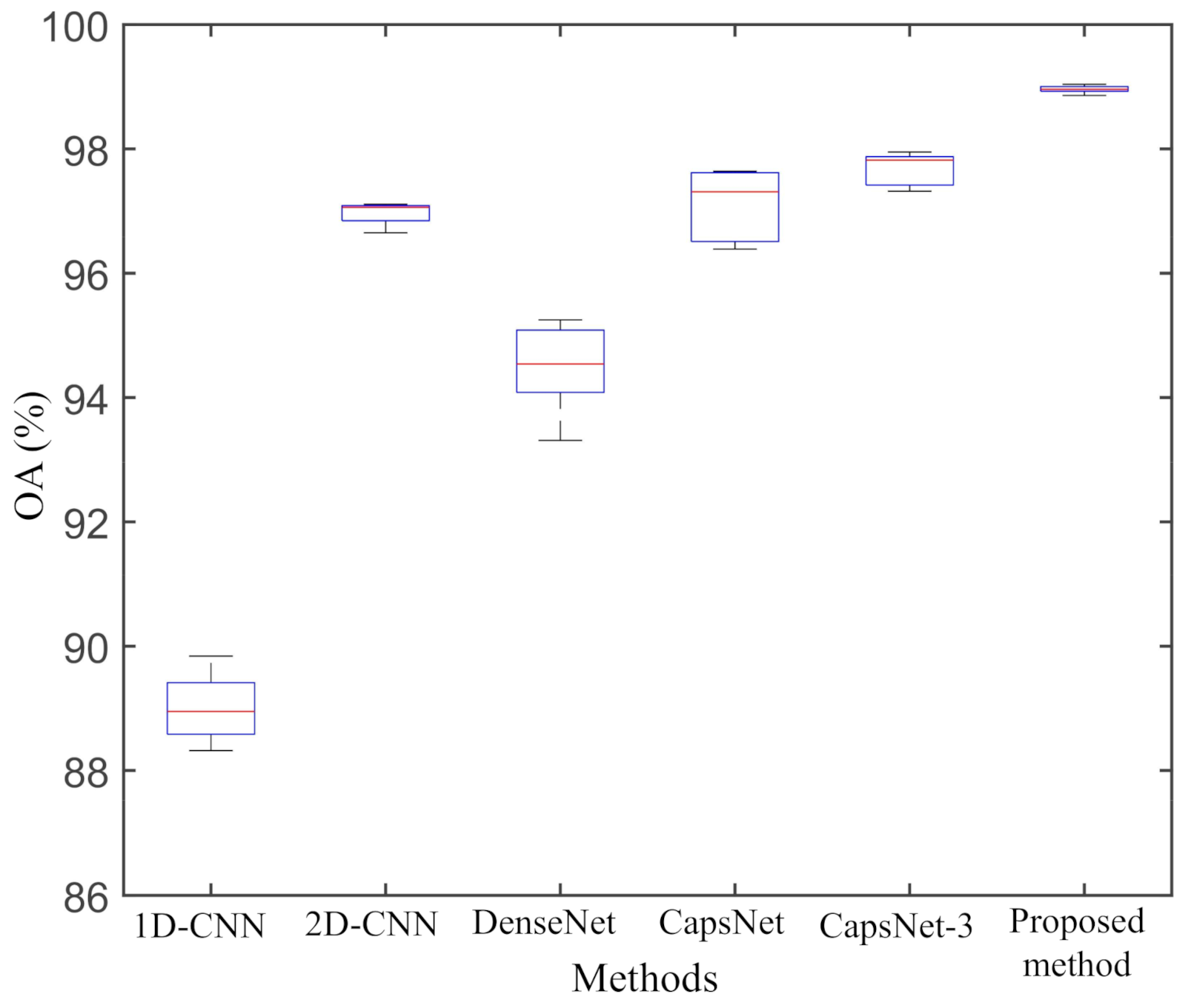
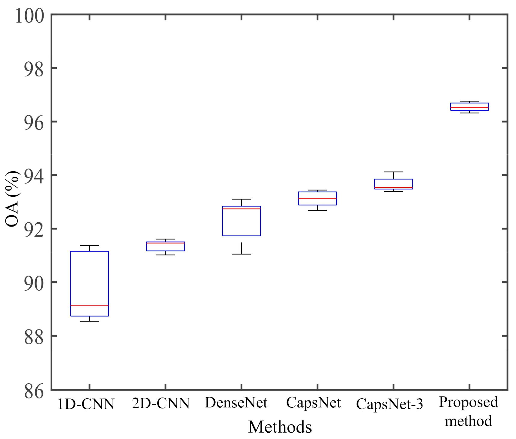
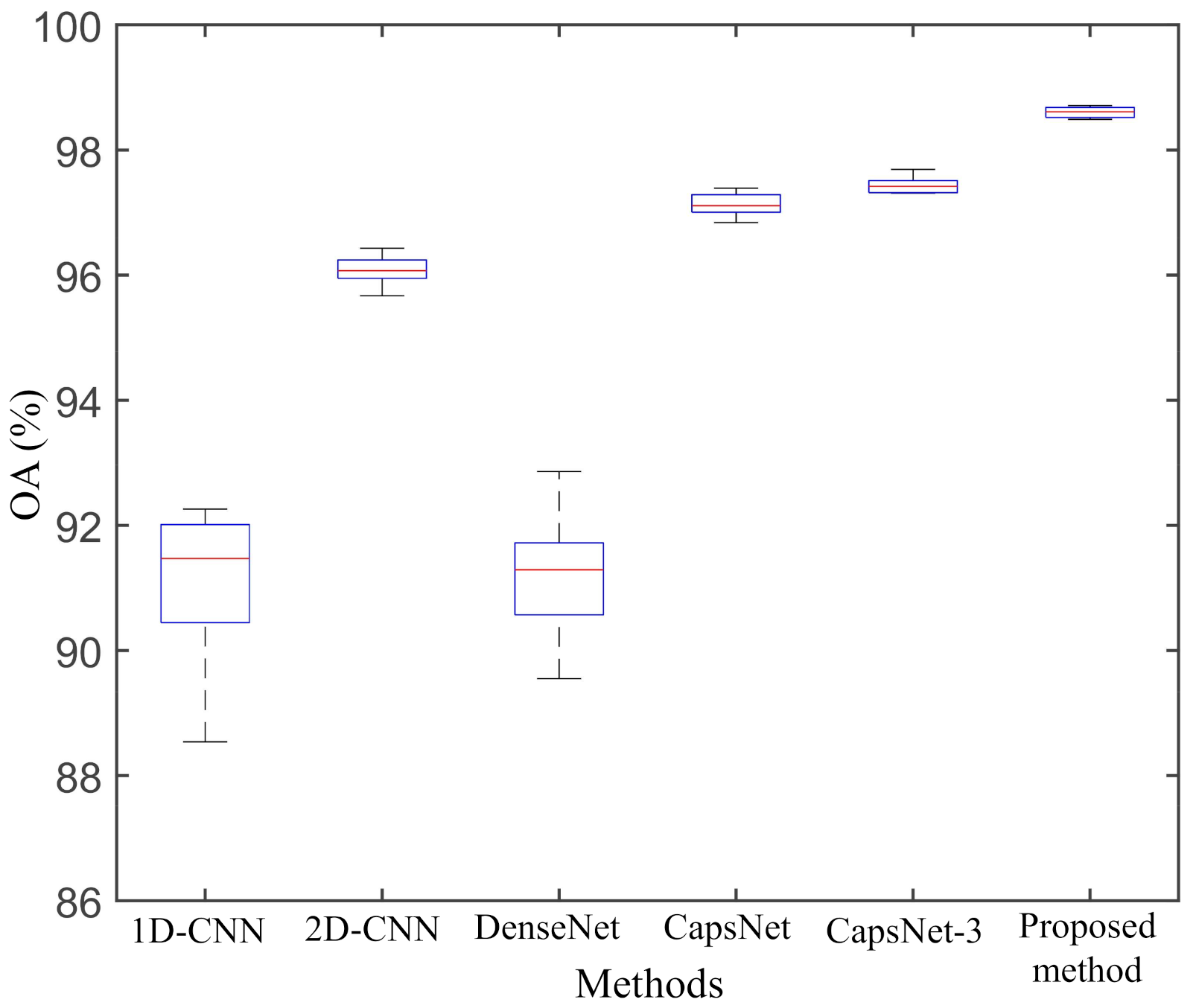
From Table 6, we can observe that our proposed method produces much higher classification accuracy than other deep neural networks. The classification accuracies of the proposed method in Rapeseed, Bare soil, Potatoes, Wheat, Wheat2, Peas, Wheat3, Lucernes, Beets, Water, and Forest are higher than other methods in L-band AIRSAR dataset. The Kappa of the proposed method is 0.9889, which is also higher than other classification methods. Figure 9 shows a box plot of five experimental results for each classification method. The height of the box represents the divergence of the results. The proposed method is superior to other classification methods in stability. The OA of the proposed method is , , , , and higher than that of 1D-CNN, 2D-CNN, DenseNet, CapsNet, and CapsNet-3, respectively. The AA of the proposed method is , , , , and higher than that of 1D-CNN, 2D-CNN, DenseNet, CapsNet, and CapsNet-3, respectively.
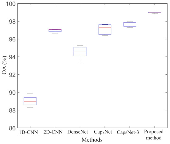
Figure 9.
Box plot of the five repeated experimental results on AIRSAR Flevoland dataset.
In the AIRSAR Flevoland dataset, wheat is subdivided into the Wheat, Wheat2, and Wheat3 regions, all of which have similar scattering mechanisms. The classification accuracy of Wheat2 can only reach to with other classification methods, while it reaches with the proposed method. This result indicates that the proposed method can perform well in distinguishing different land covers with similar scattering mechanisms than other classification methods.
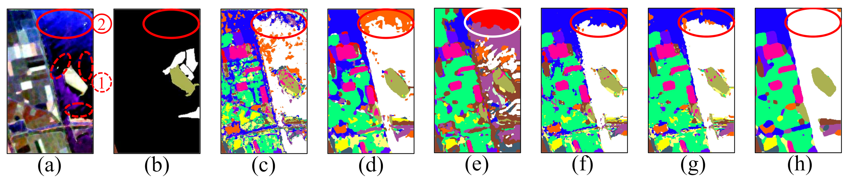
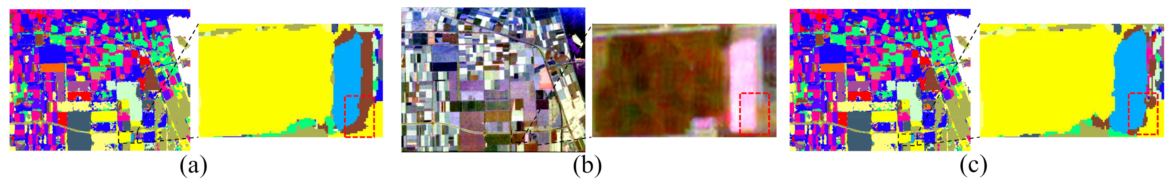
Note that in Figure 8A–E, the top of the Water region has different degrees of misclassifications. This is because the top and bottom of the Water region have some different scattering mechanisms, as shown in Figure 10a. It is difficult to completely describe the scattering mechanism of region ② by only using training samples in region ①. However, in Figure 10h, we are excited to find that the entire Water region achieves accurate classification. This result indicates that the proposed method can more comprehensively describe the different scattering mechanisms of the same land cover.
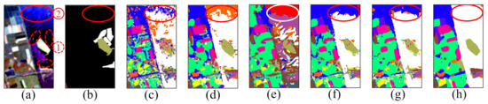
Figure 10.
Enlarged results of the Water region on AIRSAR Flevoland dataset. (a) Pauli image. (b) Ground truth map. (c) 1D-CNN. (d) 2D-CNN. (e) DenseNet. (f) CapsNet. (g) CapsNet-3. (h) Proposed method.
The classification accuracy of 1D-CNN is the lowest because the neighborhood information is not used. As shown in Figure 8a, we can observe that the misclassification is sever in the whole image. From Table 6, it can be found that although DenseNet considers the neighborhood information of the training samples, the classification results are lower than 2D-CNN, especially the classification accuracy of the Buildings region with fewer labeled samples, which is only . This result once again demonstrates that a small number of training samples cannot be suitable for training deep CNNs. Figure 8b shows that the misclassification is mainly concentrated at the class boundaries, while this phenomenon is well avoided in Figure 8f. To more intuitively show the advantages of the proposed method in class boundaries, we have enlarged the classification result maps of the Peas region, as shown in Figure 11. We can observe that the classification results of the proposed method are more consistent with the actual distribution in the Peas region.
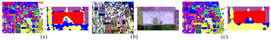
Figure 11.
Enlarged classification results of the Peas region on AIRSAR Flevoland dataset. (a) 2D-CNN. (b) Pauli RGB image. (c) Proposed method.
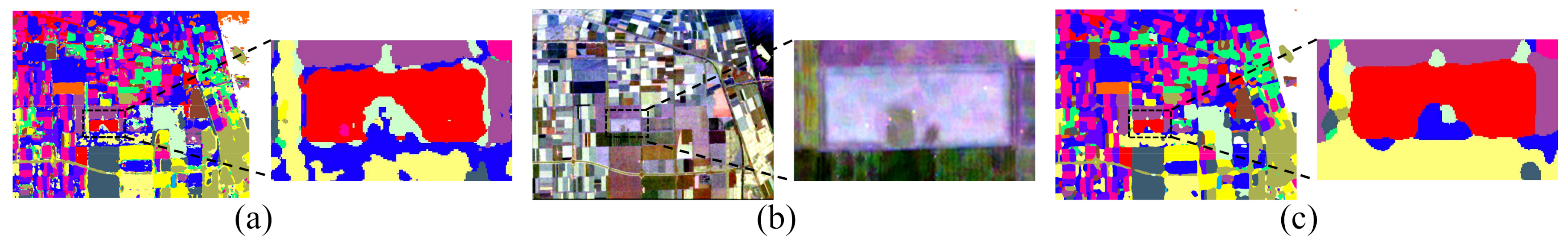
Compared with the CapsNet, the OA and AA of the CapsNet-3 have increments with and , respectively. Note that the improvement of classification accuracy is concentrated on the land cover with a small sample size. For example, compared to the CapsNet, the CapsNet-3 is higher in the classification of the Buildings region. Figure 12 shows the enlarged results of the Buildings region with the two methods. It is shown that the CapsNet has more misclassifications on boundaries of land covers with small samples than CapsNet-3. In this experiment, the number of parameters of CapsNet is about 2.82 M, whereas that of CpasNet-3 is about 1.02 M. Experiments show that reducing the dimension of higher-level capsules can not only reduces the number of parameters, but also improves the classification accuracy. In this experiment, we measure the training time of all codes (with 200 epoches). The 1D-CNN has the shortest training time, only 60 s. The training time of 2D-CNN and DenseNet is about 300 s and 150 s, respectively. The CapsNet and CapsNet-3 require about 1150 s and 1000 s to run code because of the complex dynamic routing connection used. In our method, we increase the stride of the convolutional layers and shorten the distance of backpropagation, so the training time of the proposed method is only 470 s.
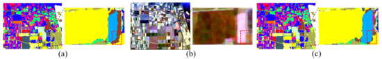
Figure 12.
Enlarged results of the Buildings region on AIRSAR Flevoland dataset. (a) CapsNet. (b) Pauli RGB image. (c) CapsNet-3.
3.3. Classification Results of the AIRSAR San Francisco Dataset
To verify the proposed method on the challenging PolSAR image, we further subdivide the human-made areas in the AIRSAR San Francisco dataset into three categories: High-density urban, Developed urban, and Low-density urban. Note that in the classic ground truth of AIRSAR San Francisco, these human-made areas are labeled as a whole. The classification maps are shown in the Figure 13. Table 4 shows the classification accuracies of each class with different classification methods, as well as the OA, AA, and Kappa of the AIRSAR San Francisco dataset classification results.
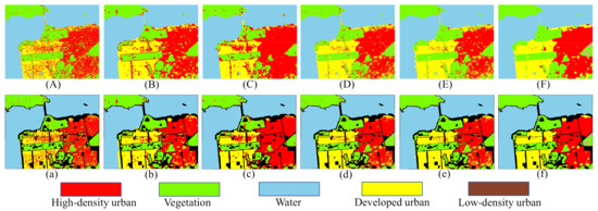
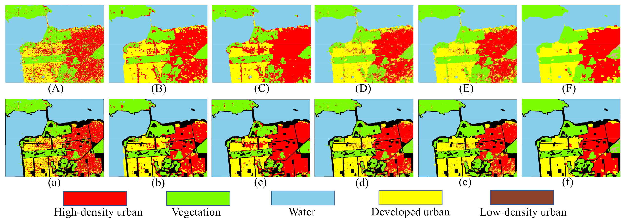
Figure 13.
Classification maps of the AIRSAR San Francisco dataset. (A) 1D-CNN. (B) 2D-CNN. (C) DenseNet. (D) CapsNet. (E) CapsNet-3. (F) Proposed method. (a–f) are the masked results according to the ground truth of (A), (B), (C), (D), (E), and (F), respectively.
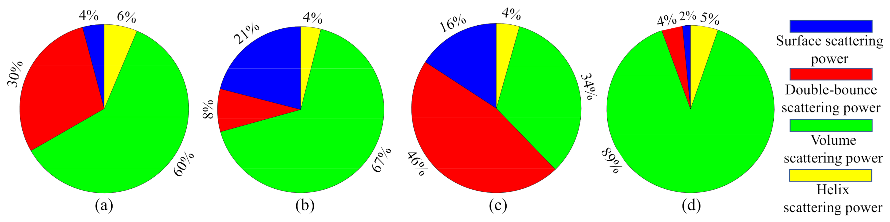
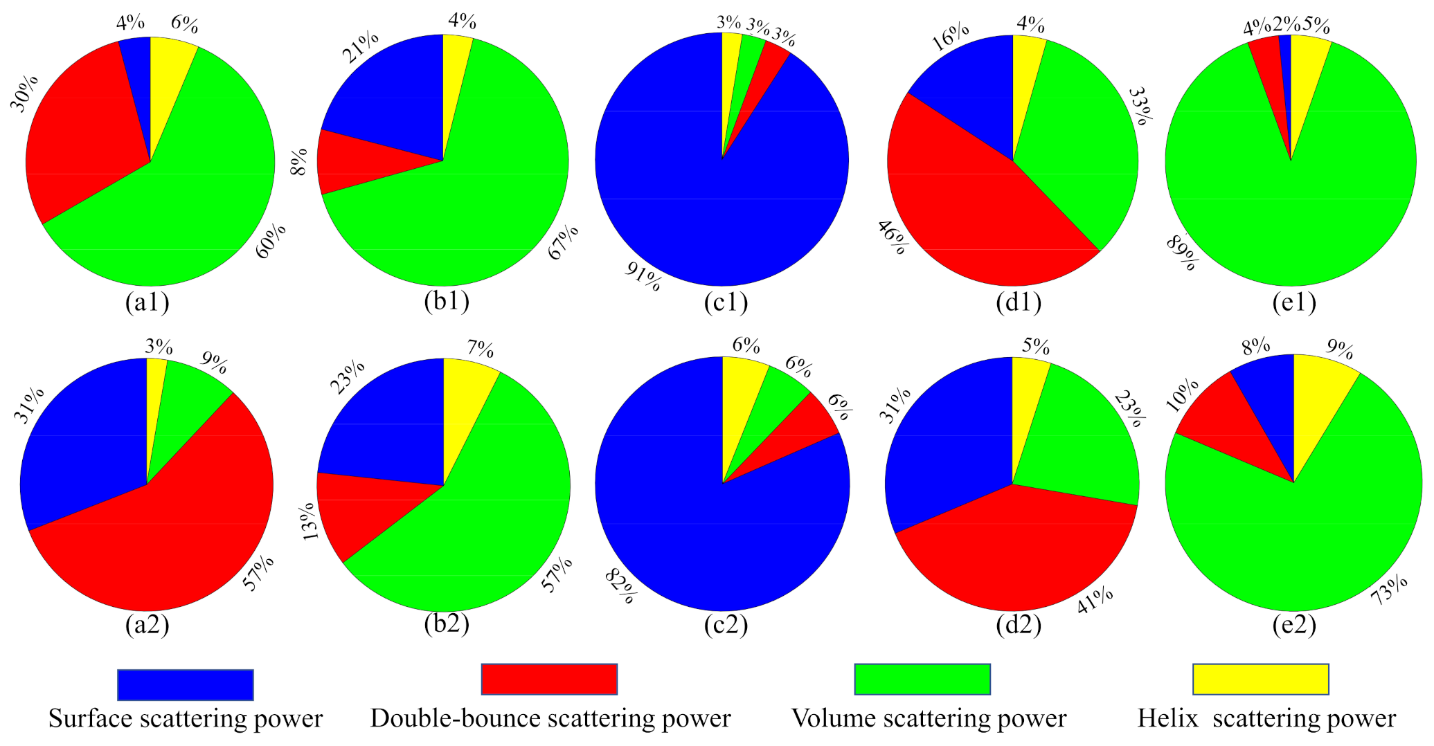
From Figure 14, we can see that the proposed method achieves the highest classification accuracy and stability in the AIRSAR San Francisco dataset. Figure 13A shows that the misclassifications are sever in the whole images. As shown in Figure 13B,C, the three human-made areas are seriously misclassified. As shown in Figure 13D,E, misclassifications of Vegetation and urban areas has been significantly improved. Note that in Figure 13a–e, most of the Low-density urban area is misclassified as Vegetation. This is because the scattering mechanism of Low-density urban is closer to that of Vegetation [55]. As we all know, buildings will produce double-bounce scattering with the ground, which is an important feature to distinguish human-made regions. Figure 15 shows the composition of the scattering mechanism in different regions (calculated based on Yamaguchi four-component decomposition [56]). In Figure 15, double-bounce scattering occupies an important proportion in Developed urban and High-density urban, but a very small proportion in Low-density urban, resulting in Low-density urban being wrongly classified as Vegetation. From Figure 13f), we can observe that a part of Low-density urban can be separated from Vegetation. This show that our proposed method can extract the discriminative features of Low-density urban and Vegetation.
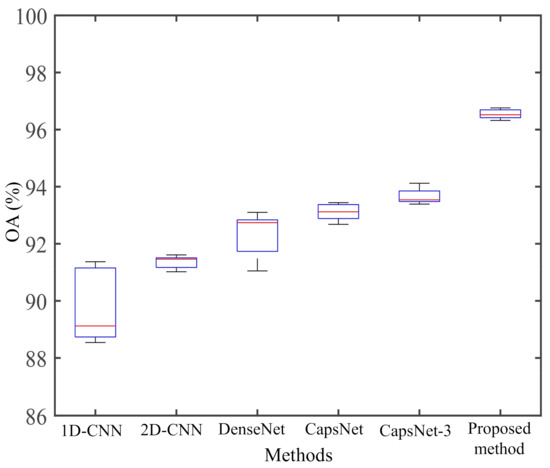
Figure 14.
Box plot of the five repeated experimental results on AIRSAR San Francisco dataset.
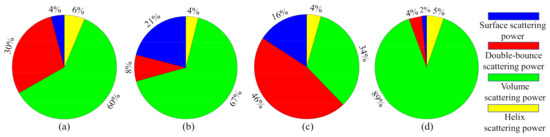
Figure 15.
Illustration of scattering mechanism in different regions. (a) High-density urban. (b) Vegetation. (c) Developed urban. (d) Low-density urban.
From Table 7, we can find that the classification accuracies of the proposed method in Vegetation, Water, Developed urban, Low-density urban are higher than other classification methods. The classification accuracy of Low-density urban is in 1D-CNN, 2D-CNN, and DenseNet results, which shows that the 1D-CNN, 2D-CNN, and DenseNet are completely unable to learn the difference in scattering mechanism between low-density urban and vegetation. The OA of the proposed method is , , , , and higher than that of 1D-CNN, 2D-CNN, DenseNet, CapsNet, and CapsNet-3, respectively. The AA of the proposed method is , , , , and higher than that of 1D-CNN, 2D-CNN, DenseNet, CapsNet and CapsNet-3, respectively.
Table 7.
Classification accuracy (%) of the AIRSAR San Francisco Dataset.
Compared with the CapsNet, the OA of the CapsNet-3 has increments with . This shown that the CapsNet-3 performs better in the classification of land covers than the CapsNet. In addition, we also measure the training time of the codes on the GF-3 dataset. The training time of 1D-CNN, 2D-CNN, DenseNet, CapsNet, and CapsNet-3 are about 156 s, 364 s, 366 s, 1120 s and 1043 s, respectively. Compare with the traditional CapsNet, the training time of the proposed method is only about 490 s.
3.4. Classification Results of the GF-3 Dataset
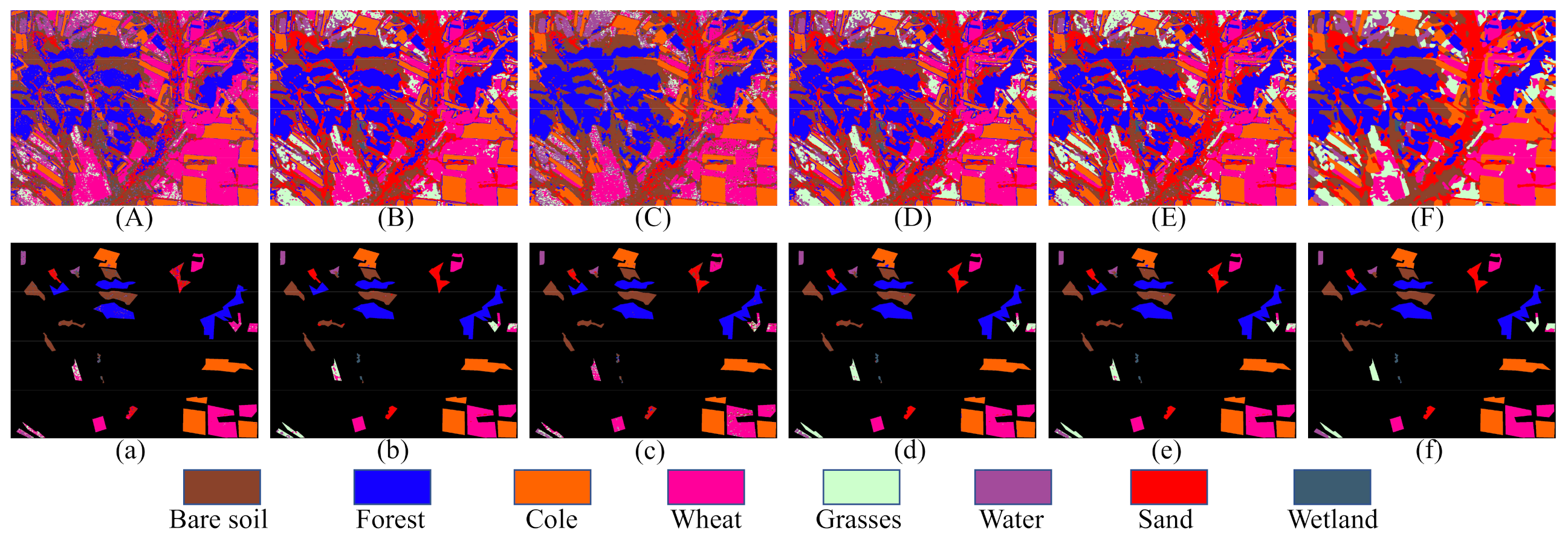
To verify the effectiveness of the proposed method, comparison experiments are also conveyed on the GF-3 dataset. As the GF-3 dataset has few categories and relatively simple image scene, only of the labeled samples are selected as training samples. The experiments are repeated five times, and the average value was taken as the final classification result. The classification maps are shown in the Figure 16. Table 8 shows the classification accuracies of each class with different classification methods, as well as the OA, AA, and Kappa of the GF-3 dataset classification results.
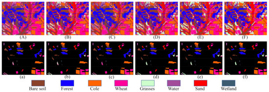
Figure 16.
Classification maps of the GF-3 dataset. (A) 1D-CNN. (B) 2D-CNN. (C) DenseNet. (D) CapsNet. (E) CapsNet-3. (F) Proposed method. (a–f) are the masked results according to the ground truth of (A), (B), (C), (D), (E), and (F), respectively.
Table 8.
Classification Accuracy (%) of the GF-3 Dataset.
From Figure 16 and Figure 17, we can see that the proposed method once again achieves the highest classification accuracy and stability in the GF-3 dataset. From Table 8, we can observe that the classification accuracies of the proposed method in Forest, Cole, Wheat, Grasses, Water, and Sand are higher than other classification methods. Figure 16A,B shows that the misclassifications are severe in the whole images. The classification results of 1D-CNN and DenseNet are relatively poor, especially the classification accuracies of Grasses are only and . In the case of a very small number of training samples, 2D-CNN exposed its shortcomings, that the classification accuracies of Grasses and Water are only and , respectively. From Table 8, we can see that the AA of the proposed method is , , , , and higher than that of 1D-CNN, 2D-CNN, DenseNet, CapsNet, and CapsNet-3, respectively.
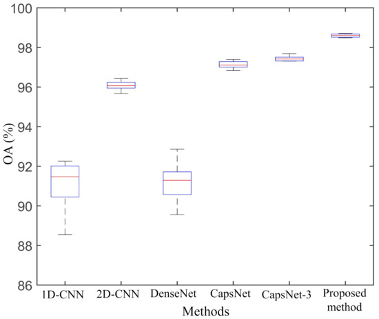
Figure 17.
Box plot of the five repeated experimental results on GF-3 dataset.
In PolSAR image classification, the same scattering mechanism can represent different land covers. For example, the main scattering mechanisms of Bare soil and Sand are both surface scattering. As shown in Figure 8a–e, many pixels of Sand are misclassified as Bare soil. The misclassifications are well solved in Figure 16f. The classification accuracy of the Sand in the proposed method is about to higher than other classification methods. This result once again proves that the proposed method can extract more discriminative features from different land covers with similar scattering mechanisms. In addition, despite the large number of training samples for Grasses and Water, the scattering mechanism of Grasses is confused with Wheat, and the scattering mechanism of Water is confused with Bare soil, so the classification accuracy of Grasses and Water is lower than other land covers.
Compared with the CapsNet, the OA and AA of the CapsNet-3 have increments with and , respectively. The CapsNet-3 performs better in the classification of land covers with small sample size than the CapsNet. The classification results of three PolSAR datasets both indicate that reducing the dimension of higher-level capsules has a positive effect on improving the classification accuracy. In addition, we also measure the training time of the codes on the GF-3 dataset. The training time of 1D-CNN, 2D-CNN, DenseNet, CapsNet, and CapsNet-3 are about 13 s, 25 s, 25 s, 68 s, and 65 s, respectively. The training time of the proposed method is about 70s. Due to the small number of training samples, the saving time of the model is longer than the training time.
3.5. Analysis of the Performance
To make a fair comparison of deep learning models, we make their structures and parameter settings near identical. CNN-CapsNet [28] indicates that the fully connected layers in the 2D-CNN are replaced with the capsule layers. The proposed HCapsNet implements a hierarchical capsule network structure based on the CNN-CapsNet. Herein, only the results for the AIRSAR Flevoland dataset are presented, while similar conclusions are obtained from the AIRSAR San Francisco and GF-3 datasets. Table 9 gives a brief description of their architectures.
Table 9.
A brief description of structures and parameters.
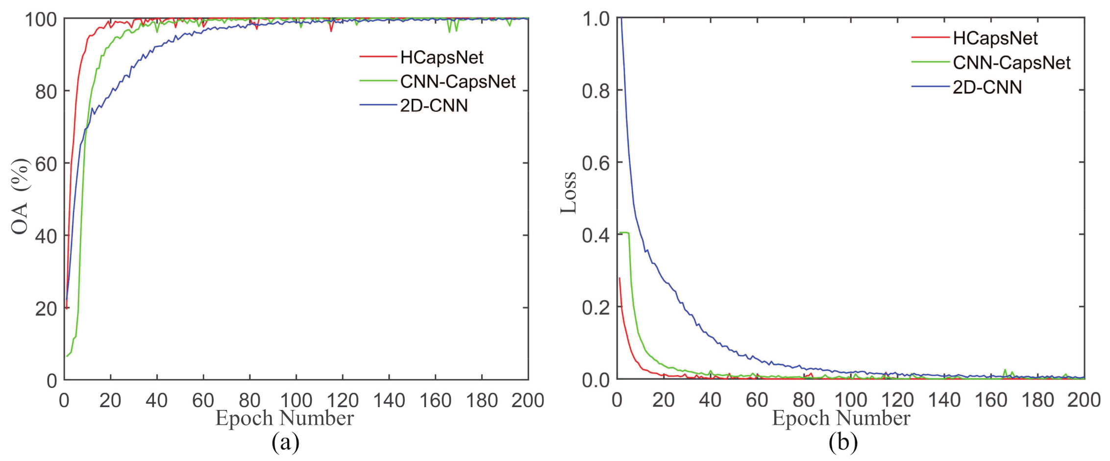
Figure 18 shows the convergence performance of the three methods on the AIRSAR dataset. As shown in Figure 18a, we can find that the proposed HCapsNet can quickly reach a high accuracy. The reason is that capsule networks turn the traditional neuron output into the vector output of the capsule, which can simultaneously represent multiple polarimetric attributes of land covers. Therefore, it can be in line with the scattering characteristics of actual land covers. As shown in Figure 18b, we can observe that 2D-CNN can completely converge in about 140 epochs, CNN-CapsNet can completely converge in about 80 epochs. In contrast, the proposed method can completely converge in about 40 epochs. The reason is that the proposed HCapsNet can shorten the distance of backpropagation, resulting in that the loss of the primary capsule layer to reach the input layer and each convolutional layer directly.
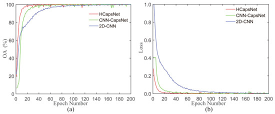
Figure 18.
The loss and accuracy curves of different methods variation with iteration increasing.
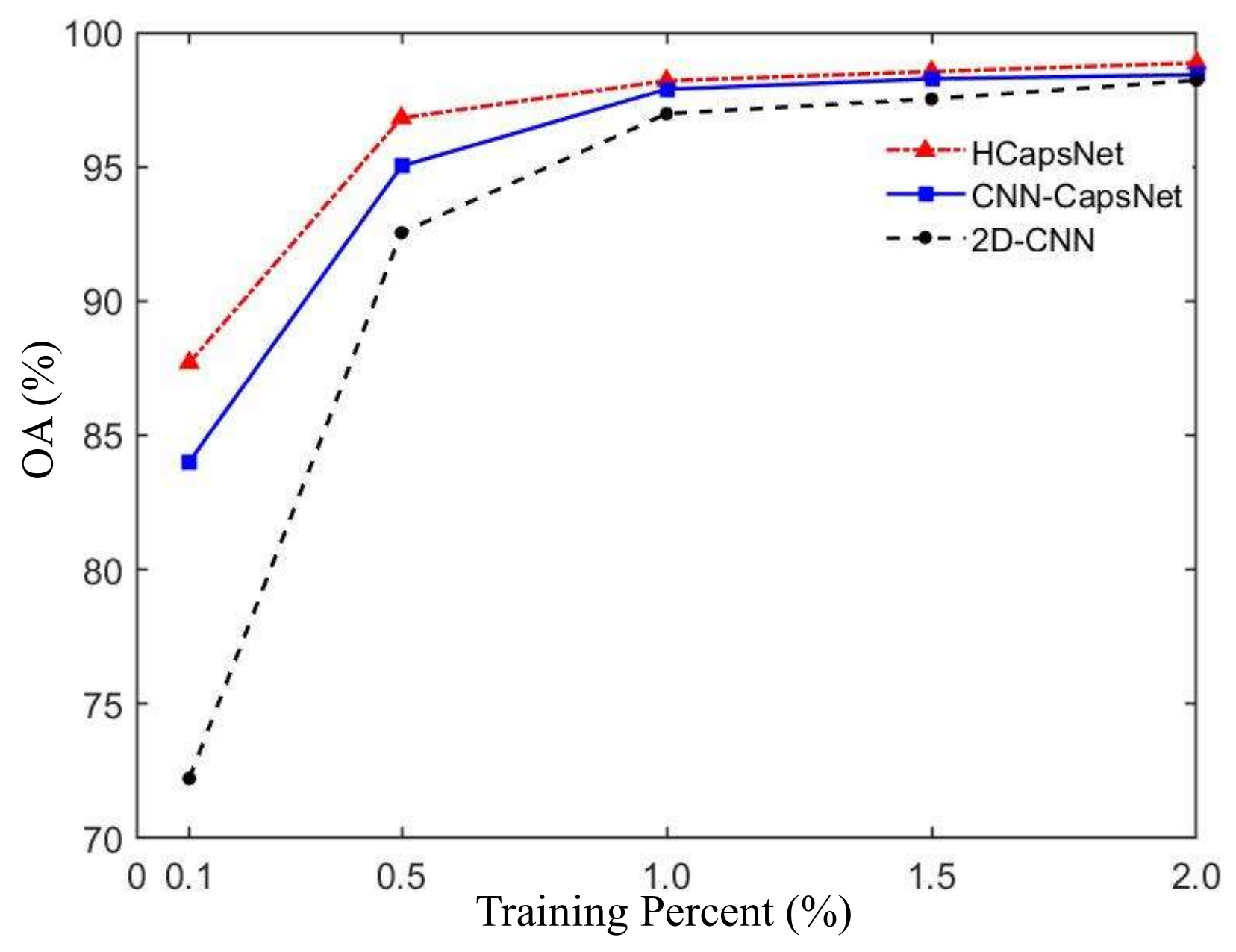
The rapid convergence of deep learning algorithms depends on their powerful feature learning capabilities. This means that the algorithm can learn useful features from a small size of training samples. Figure 19 shows the OA of the three classification methods at , , , , and training sample ratio. We can see that in the case of enough training samples (), the OA of the proposed HCapsNet is slightly higher than CNN-CapsNet and 2D-CNN. When the training sample ratio is only , the proposed HCapsNet can still maintain more than classification accuracy without any postprocessing. With the reduction of training samples, the classification accuracy of 2D-CNN decreases faster. When the training sample ratio is only , the classification accuracy of 2D-CNN is much lower than that of the CNN-CapsNet and HCapsNet. Regardless of the ratio of training samples, the proposed HCapsNet can obtain the highest classification accuracy.
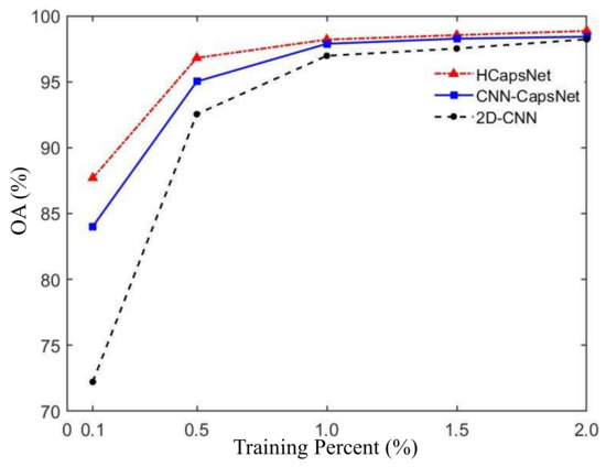
Figure 19.
Classification accuracies with different training percentages on AIRSAR Flevoland data.
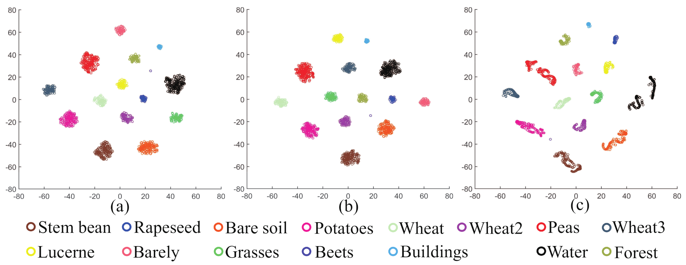
The proposed method achieves the highest accuracy compared with the other classification methods on the three PolSAR datasets. This means that the proposed method can learn more discriminative features from PolSAR images. A good discriminative feature should have two aspects, one is high degree of inter-class dispersion and another is high degree of intra-class concentration. Figure 20 shows the distribution of training results with a scattering plot, using the t-SNE technology for dimensionality reduction. As shown in Figure 20c, in the training results of 2D-CNN, the deep features are not discriminative enough, as they still show significant intra-class variations. As shown in Figure 20a,b, the distribution of the training samples has high inter-class separation and intra-class concentration.

Figure 20.
Visualization of data distribution with different methods. (a) HCapsNet. (b) CNN-CapsNet. (c) 2D-CNN.
To verify the effectiveness of the proposed method, the proposed method is compared with state-of-the-art methods in the PolSAR image classification field. The training sample rate in the comparison experiments is also set as . Four methods are selected for comparison: the multichannel fusion convolutional neural network based on scattering mechanism (MCCNN) [52], the compact and adaptive implementation of CNNs using a sliding-window classification approach [57], the composite kernel and Hybrid discriminative random field model based on feature fusion (CK-HDRF) [58], and the recurrent complex-valued convolutional neural network (RCV-CNN) [13]. In which, CK-HDRF belongs to machine learning, RCV-CNN belongs to semi-supervised learning. Table 10 shows the OA, AA, and Kappa of the AIRSAR Flevoland classification results. As can be seen from Table 10, under the condition of limited training samples (), it is difficult to achieve classification accuracy even with state-of-the-art classification methods. However, the OA of our proposed HCapsNet can easily reach without CRF. Furthermore, with CRF optimization, the OA of our proposed method can even reach .
Table 10.
Classification accuracy comparison of state-of-the-art methods on the AIRSAR Flevoland dataset.
In summary, the convergence speed of the proposed method is faster than the CNN-CapsNet, while the convergence speed of the CNN-CapsNeet is faster than the 2D-CNN. The small sample performance of the proposed method is superior than the CNN-CapsNet and the 2D-CNN. The two CapsNets can extract more discriminative deep features than the 2D-CNN. Moreover, the proposed method outperforms other state-of-the-art methods.
4. Discussion
4.1. Contributions of Polarimetric Features
Generally, the classification performance of PolSAR images depends on the number and scattering information of input polarimetric features. In this paper, the proposed method uses three discriminative attributes, i.e., phase, amplitude, and polarimetric decomposition, to uniformly describe the scattering mechanism of different land covers. The phase and amplitude are the basic attributes of PolSAR data, which can be easily obtained from the original information of PolSAR data, which has strong application value as the input of the network, so we do not change their features. To explore the impacts of different categories and numbers of polarimetric features on the classification results, we replace the eigenvalue decomposition features with model-based decomposition features. The number of polarimetric features is increased to 9. The experiment adds the polarimetric features obtained by Yamaguchi 4-component decomposition [56], including surface scattering power (), double-bounce scattering power (), volume scattering power (), and helix scattering power (). Table 11 lists the second experimental polarimetric feature set.
Table 11.
The Polarimetric Feature Set II.
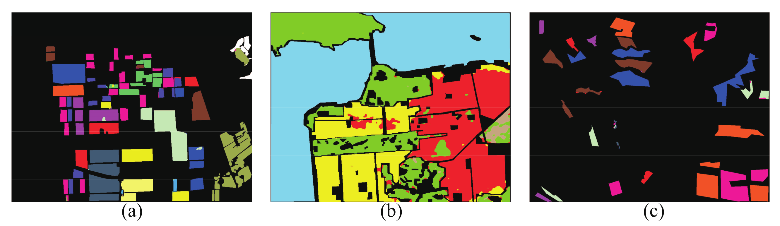
As shown in Figure 21, we can see that the proposed method, with polarimetric feature set II, still achieves good classification results on the three PolSAR datasets. We calculate the quantitative evaluations of the classification results for the three PolSAR datasets. The OA, AA, and Kappa of the AIRSAR Flevoland dataset are , , and 0.9882, respectively. The OA, AA, and Kappa of the AIRSAR San Francisco dataset are , , and 0.9534, respectively. The OA, AA, and Kappa of the GF-3 dataset are , , and 0.9935, respectively. The experimental results indicate that the proposed method is robust to changes in the number and category of input polarimetric features.
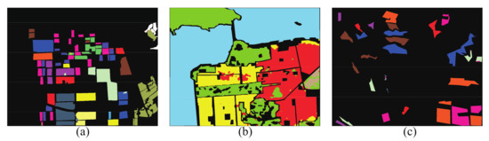
Figure 21.
Classification maps of proposed method with polarimetric Feature Set II. (a) AIRSAR Flevoland dataset. (b) AIRSAR San Francisco dataset. (c) GF-3 dataset.
4.2. Comparison of Different Feature Extractors
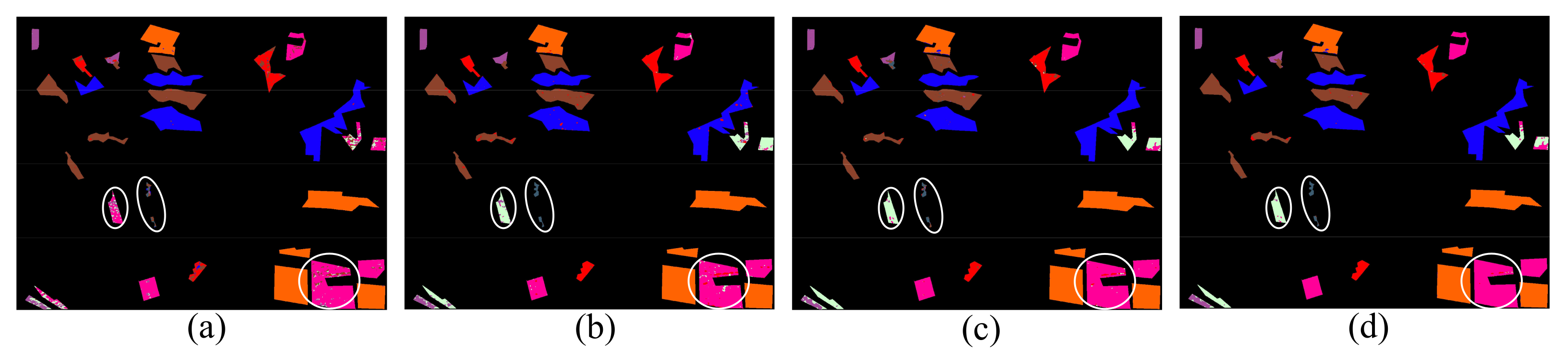
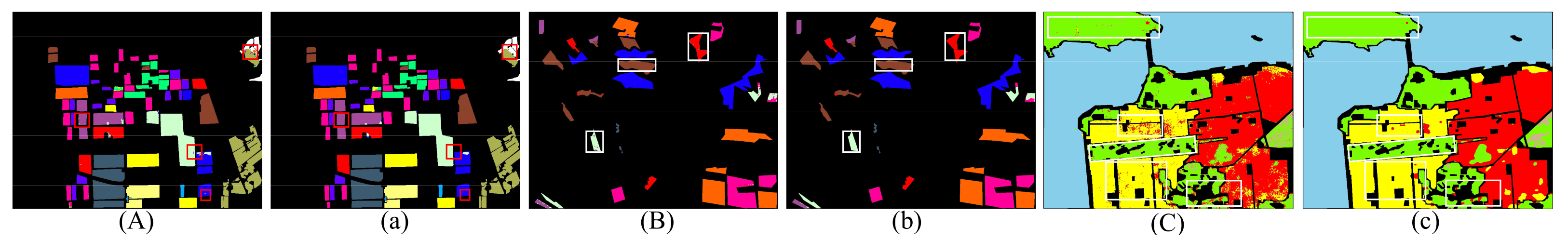
The traditional CapsNet is insufficient in the deep feature extraction capability. In the field of remote sensing image application, researchers have improved the feature extractor of the capsule network, such as residual capsule network (Res-CapsNet) [21], densely connected capsule network (Dense-CapsNet) [26], and CNN-CapsNet [28]. We apply these methods to the land cover classification of PolSAR images and compare them with the proposed method. For the sake of fair comparison, all methods use the same training samples and test samples, and do not use postprocessing (without CRF). The experiments are repeated five times, and the average value is taken as the final result. The classification maps are shown in the Figure 22, Figure 23 and Figure 24. The OA, AA, and Kappa of classification results with different classification methods are shown in Table 12.

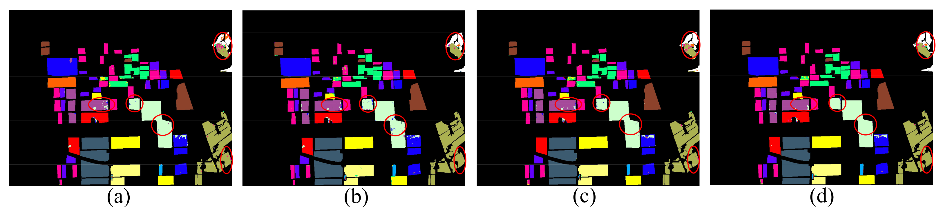
Figure 22.
Classification maps of AIRSAR Flevoland dataset with different classification methods. (a) Dense-CapsNet. (b) Res-CapsNet. (c) CNN-CapsNet. (d) Proposed HCapsNet (without CRF).
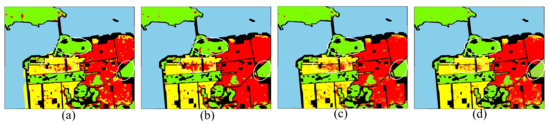
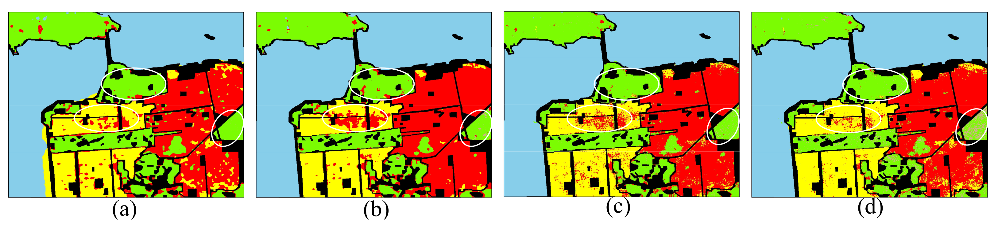
Figure 23.
Classification maps of AIRSAR San Francisco dataset with different classification methods. (a) Dense-CapsNet. (b) Res-CapsNet. (c) CNN-CapsNet. (d) Proposed HCapsNet (without CRF).
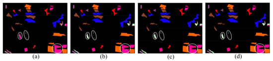
Figure 24.
Classification maps of GF-3 dataset with different classification methods. (a) Dense-CapsNet. (b) Res-CapsNet. (c) CNN-CapsNet. (d) Proposed HCapsNet (without CRF).
Table 12.
Comparison of the classification accuracy with different methods.
From Table 12, we can observe that the Dense-CapsNet has the lowest classification accuracy of the three PolSAR datasets, especially in the classification results of the GF-3 dataset, the OA is , while the AA is only . This means that the Dense-CapsNet has poor classification accuracy on land cover with a small sample size. In the classification results of the AIRSAR Flevoland dataset, the AA of the proposed HCapsNet is higher than that of the Dense-CapsNet, Res-CapsNet, and CNN-CapsNet by , , and , respectively. In the classification results of the AIRSAR San Francisco dataset, the AA of the proposed HCapsNet is higher than that of the Dense-CapsNet, Res-CapsNet, and CNN-CapsNet by , , and , respectively. In the classification results of the GF-3 dataset, the AA of the proposed HCapsNet is higher than that of the Dense-CapsNet, Res-CapsNet, and CNN-CapsNet by , , and , respectively. To show the results more intuitively, we mark important regions to compare the classification results of different methods. We can observe that the HCapsNet can significantly reduce the misclassifications of class boundaries.
4.3. Effect of the CRF
In this part, we discuss the effect of the CRF on the classification results. CRF can eliminate small isolated regions of the classification results and further improve the classification accuracy. To intuitively show the impacts of the CRF, we mark the classification maps, as shown in Figure 25. We can find that the CRF significantly reduces the intra-class misclassification. In the classification maps with the CRF, as shown in Figure 25a–c, there are almost no isolated misclassified pixels.
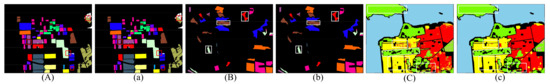
Figure 25.
(A–C) Classification maps of the proposed HCapsNet without the CRF. (a–c) Classification maps of the proposed HCapsNet with the CRF.
4.4. Generalization Performance
As is well known, the majority of deep learning-based classification methods have poor generalization performance. This is because the learned classification rules by these methods deviate from the real scattering mechanism of land covers. In addition, the large differences in the scattering mechanism of land covers in PolSAR images with different sensors, band, and resolutions. In this paper, we design three discriminative attributes, i.e., phase, amplitude, and polarimetric decomposition parameters, to uniformly describe the scattering mechanism of land covers with different sensors, bands, and resolutions. Moreover, we propose HCapsNet to accurately describe the scattering mechanism of land covers.
The trained model distinguishes different land covers based on differences between the scattering mechanisms of land covers. Therefore, the trained model is suitable for transfer only when the two datasets contain same land covers with similar scattering mechanisms. Furthermore, to make the trained model transfer effective, we use the same filtering and feature normalization processing on the new dataset, and select sensors with similar resolutions. The new San Francisco dataset is acquired by the RADARSAT-2 system in 2008. The spatial resolution is 8 m. Figure 26 is a pseudo-color image formed by PauliRGB decomposition. The size of experimental region is . There are also five categories of land covers as same as the AIRSAR Flevoland dataset, i.e., High-density urban, Vegetation, Water, Developed urban, and Low-density urban. From Figure 27, we can observe that in the scattering mechanisms of Developed urban in the AIRSAR dataset correspond to the Developed urban and High-density urban in the RS2 dataset [59,60,61]. In addition, the proportions of scattering mechanisms of different land covers in two datasets are shown in Figure 28. We can observe that in High-density urban and Developed urban, double-bounce scattering power occupies an important proportion [55]. In these two datasets, Vegetation, Water, and Low-density urban have similar scattering mechanism proportions.
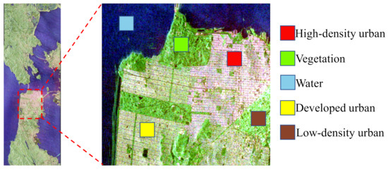
Figure 26.
PauliRGB image of RS2 San Francisco dataset (Red: double-bounce scattering power. Green: volume scattering power. Blue: surface scattering power).
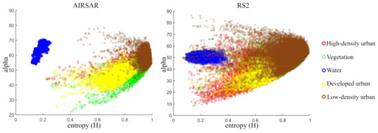
Figure 27.
H-Alpha plots of two San Francisco datasets.
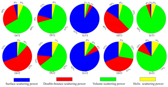
Figure 28.
Comparison of the scattering mechanism of different land covers with different sensors. (a1,a2) are High-density urban. (b1,b2) are Vegetation. (c1,c2) are Water. (d1,d2) are Developed urban. (e1,e2) are Low-density urban. (a1–e1) are the results of the AIRSAR sensor. (a2–b2) are the results of the RS2 sensor.
From Figure 29a, we can find that the positions of Developed urban and High-density urban are completely reversed, and large regions of Vegetation are misclassified as High-density urban. The 1D-CNN classification method even misclassifies Water into Vegetation. In Figure 29b, a lot of human-made regions are misclassified into Water, which shows that 2D-CNN cannot learn the correct scattering mechanism of land covers. In Figure 29c,d, a lot of Vegetation regions are misclassified into High-density urban. In CapsNet-3 classification method, we set the number of attributes of land covers as 3, which is equal to the number of categories of the input polarimetric features. Therefore, the generalization performance of the model has significantly improved, as shown in Figure 29e. In Figure 29f, human-made regions and non-human-made regions can be well separated, and a part of Low-density urban can be correctly classified. Admittedly, all the classification models cannot correctly classify the Developed urban and High-density urban. This is because the scattering mechanisms of the Developed urban in AIRSAR dataset and High-density urban in RS2 dataset are particularly similar, as shown in Figure 28a2,d1.
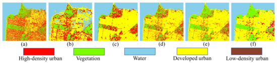
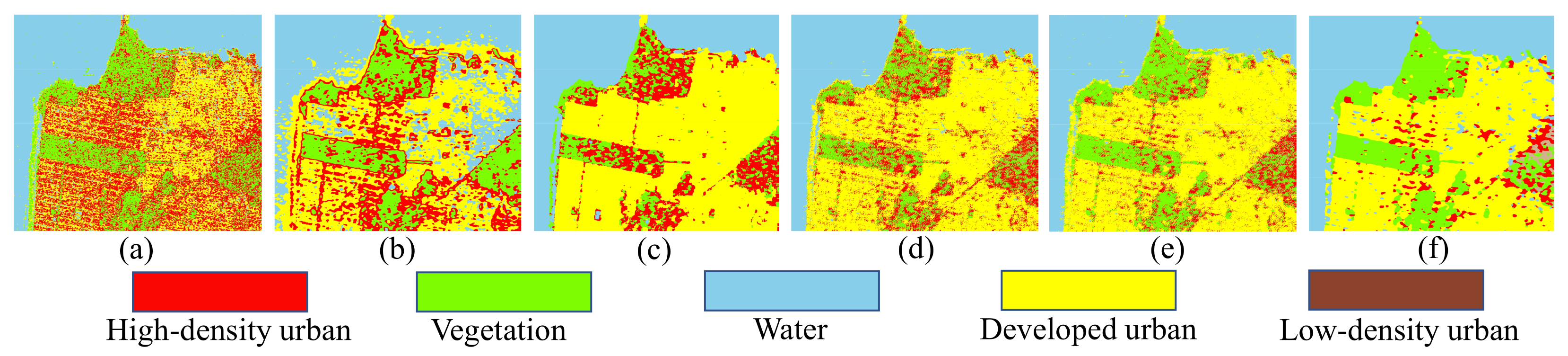
Figure 29.
Classification maps of the RS2 dataset. (a) 1D-CNN. (b) 2D-CNN. (c) DenseNet. (d) CapsNet. (e) CapsNet-3. (f) Proposed method.
In general, our proposed method can show good generalization performance on datasets with similar scattering mechanisms and similar resolutions. This is a very meaningful study that proves the generalization performance of the proposed method and the deep features extracted by the proposed method follow the scattering mechanism of land covers.
5. Conclusions
In this paper, we proposed a PolSAR image land cover classification method, called the hierarchical capsule network (HCapsNet). HCapsNet can consider the deep features obtained at different network levels and jointly represent multiple scattering mechanisms of different land covers. It can describe the polarimetric scattering information of land covers more comprehensively, and significantly reduces the misclassification of class boundaries. Moreover, the CRF can eliminate small isolated regions of the classification results. Experimental results of three PolSAR datasets proved that our method can overcome this difficulty well. The proposed method can reach OA of the AIRSAR Flevoland dataset with a training sample ratio, and OA of the AIRSAR San Francisco dataset with a training sample ratio. In the GF-3 dataset, with a training sample ratio, the OA reached . We designed a comparable framework and prove the advantages of the proposed method in convergence speed, small sample performance, and feature learning ability. Furthermore, we proved that the proposed method is robust to changes in the number and category of input polarimetric features. In addition, we conducted transfer tests on the trained models, confirming that the generalization performance of the proposed method is better than comparison methods.
Author Contributions
Conceptualization, D.X.; Methodology, J.C.; Software, J.C., Q.Y. and W.W.; Resources, F.Z., D.X. and Q.Y.; Writing, J.C. and Y.Z. All authors have read and agreed to the published version of the manuscript.
Funding
This work was supported in part by the National Natural Science Foundation of China under Grant 61871413, 41801236, 61801015, and in part by the Fundamental Research Funds for the Central Universities under Grant XK2020-03.
Acknowledgments
The authors acknowledge Erxue Chen in Chinese Academy of Forestry for providing the field type information of Gaofen-3 data.
Conflicts of Interest
The authors declare no conflict of interest.
References
- Zhang, F.; Ni, J.; Yin, Q.; Li, W.; Li, Z.; Liu, Y.; Hong, W. Nearest-regularized subspace classification for PolSAR imagery using polarimetric feature vector and spatial information. Remote Sens. 2017, 9, 1114. [Google Scholar] [CrossRef] [Green Version]
- Li, L.; Liu, X.; Chen, Q.; Yang, S. Building damage assessment from PolSAR data using texture parameters of statistical model. Comput. Geosci. 2018, 113, 115–126. [Google Scholar] [CrossRef]
- Eom, K.B. Fuzzy clustering approach in unsupervised sea-ice classification. Neurocomputing 1999, 25, 149–166. [Google Scholar] [CrossRef]
- Gomez, L.; Alvarez, L.; Mazorra, L.; Frery, A.C. Fully PolSAR image classification using machine learning techniques and reaction-diffusion systems. Neurocomputing 2017, 255, 52–60. [Google Scholar] [CrossRef]
- Xiang, D.; Ban, Y.; Wang, W.; Su, Y. Adaptive superpixel generation for polarimetric SAR images with local iterative clustering and SIRV model. IEEE Trans. Geosci. Remote Sens. 2017, 55, 3115–3131. [Google Scholar] [CrossRef]
- Guan, D.; Xiang, D.; Dong, G.; Tang, T.; Tang, X.; Kuang, G. SAR image classification by exploiting adaptive contextual information and composite kernels. IEEE Geosci. Remote Sens. Lett. 2018, 15, 1035–1039. [Google Scholar] [CrossRef]
- Yin, Q.; Cheng, J.; Zhang, F.; Zhou, Y.; Shao, L.; Hong, W. Interpretable POLSAR Image Classification Based on Adaptive-dimension Feature Space Decision Tree. IEEE Access 2020, 8, 173826–173837. [Google Scholar] [CrossRef]
- Bi, H.; Xu, L.; Cao, X.; Xue, Y.; Xu, Z. Polarimetric SAR image semantic segmentation with 3D discrete wavelet transform and Markov random field. IEEE Trans. Image Process. 2020, 29, 6601–6614. [Google Scholar] [CrossRef]
- De, S.; Bruzzone, L.; Bhattacharya, A.; Bovolo, F.; Chaudhuri, S. A novel technique based on deep learning and a synthetic target database for classification of urban areas in PolSAR data. IEEE J. Sel. Top. Appl. Earth Obs. Remote Sens. 2017, 11, 154–170. [Google Scholar] [CrossRef]
- Hariharan, S.; Mandal, D.; Tirodkar, S.; Kumar, V.; Bhattacharya, A.; Lopez-Sanchez, J.M. A novel phenology based feature subset selection technique using random forest for multitemporal PolSAR crop classification. IEEE J. Sel. Top. Appl. Earth Obs. Remote Sens. 2018, 11, 4244–4258. [Google Scholar] [CrossRef] [Green Version]
- Chen, S.W.; Tao, C.S. PolSAR image classification using polarimetric-feature-driven deep convolutional neural network. IEEE Geosci. Remote Sens. Lett. 2018, 15, 627–631. [Google Scholar] [CrossRef]
- Li, Y.; Chen, Y.; Liu, G.; Jiao, L. A novel deep fully convolutional network for PolSAR image classification. Remote Sens. 2018, 10, 1984. [Google Scholar] [CrossRef] [Green Version]
- Xie, W.; Ma, G.; Zhao, F.; Liu, H.; Zhang, L. PolSAR image classification via a novel semi-supervised recurrent complex-valued convolution neural network. Neurocomputing 2020, 388, 255–268. [Google Scholar] [CrossRef]
- Touzi, R. Target scattering decomposition in terms of roll-invariant target parameters. IEEE Trans. Geosci. Remote Sens. 2006, 45, 73–84. [Google Scholar] [CrossRef]
- Gosselin, G.; Touzi, R.; Cavayas, F. Polarimetric Radarsat-2 wetland classification using the Touzi decomposition: Case of the Lac Saint-Pierre Ramsar wetland. Can. J. Remote Sens. 2014, 39, 491–506. [Google Scholar] [CrossRef]
- Touzi, R.; Omari, K.; Sleep, B.; Jiao, X. Scattered and received wave polarization optimization for enhanced peatland classification and fire damage assessment using polarimetric PALSAR. IEEE J. Sel. Top. Appl. Earth Obs. Remote Sens. 2018, 11, 4452–4477. [Google Scholar] [CrossRef]
- Wang, H.; Magagi, R.; Goïta, K.; Trudel, M.; McNairn, H.; Powers, J. Crop phenology retrieval via polarimetric SAR decomposition and Random Forest algorithm. Remote Sens. Environ. 2019, 231, 111234. [Google Scholar] [CrossRef]
- Muhuri, A.; Manickam, S.; Bhattacharya, A. Scattering mechanism based snow cover mapping using RADARSAT-2 C-Band polarimetric SAR data. IEEE J. Sel. Top. Appl. Earth Obs. Remote Sens. 2017, 10, 3213–3224. [Google Scholar] [CrossRef]
- Wang, H.; Magagi, R.; Goita, K.; Jagdhuber, T. Refining a polarimetric decomposition of multi-angular UAVSAR time series for soil moisture retrieval over low and high vegetated agricultural fields. IEEE J. Sel. Top. Appl. Earth Obs. Remote Sens. 2019, 12, 1431–1450. [Google Scholar] [CrossRef]
- Liu, J.w.; Ding, X.h.; Lu, R.k.; Lian, Y.f.; Wang, D.z.; Luo, X.l. Multi-View Capsule Network. In International Conference on Artificial Neural Networks; Springer: Cham, Switzerland, 2019; pp. 152–165. [Google Scholar]
- Yang, S.; Lee, F.; Miao, R.; Cai, J.; Chen, L.; Yao, W.; Kotani, K.; Chen, Q. RS-CapsNet: An Advanced Capsule Network. IEEE Access 2020, 8, 85007–85018. [Google Scholar] [CrossRef]
- Cheng, X.; He, J.; He, J.; Xu, H. Cv-CapsNet: Complex-valued capsule network. IEEE Access 2019, 7, 85492–85499. [Google Scholar] [CrossRef]
- Sabour, S.; Frosst, N.; Hinton, G.E. Dynamic routing between capsules. arXiv 2017, arXiv:1710.09829. [Google Scholar]
- Hinton, G.E.; Sabour, S.; Frosst, N. Matrix capsules with EM routing. In Proceedings of the International Conference on Learning Representations, Vancouver, BC, Canada, 30 April–3 May 2018. [Google Scholar]
- Guo, Y.; Pan, Z.; Wang, M.; Wang, J.; Yang, W. Learning Capsules for SAR Target Recognition. IEEE J. Sel. Top. Appl. Earth Obs. Remote Sens. 2020, 13, 4663–4673. [Google Scholar] [CrossRef]
- Phaye, S.S.R.; Sikka, A.; Dhall, A.; Bathula, D. Dense and diverse capsule networks: Making the capsules learn better. arXiv 2018, arXiv:1805.04001. [Google Scholar]
- Wang, A.; Wang, M.; Wu, H.; Jiang, K.; Iwahori, Y. A Novel LiDAR Data Classification Algorithm Combined CapsNet with ResNet. Sensors 2020, 20, 1151. [Google Scholar] [CrossRef] [PubMed] [Green Version]
- Zhang, W.; Tang, P.; Zhao, L. Remote sensing image scene classification using CNN-CapsNet. Remote Sens. 2019, 11, 494. [Google Scholar] [CrossRef] [Green Version]
- Ma, W.; Xiong, Y.; Wu, Y.; Yang, H.; Zhang, X.; Jiao, L. Change detection in remote sensing images based on image mapping and a deep capsule network. Remote Sens. 2019, 11, 626. [Google Scholar] [CrossRef] [Green Version]
- Zhu, K.; Chen, Y.; Ghamisi, P.; Jia, X.; Benediktsson, J.A. Deep convolutional capsule network for hyperspectral image spectral and spectral-spatial classification. Remote Sens. 2019, 11, 223. [Google Scholar] [CrossRef] [Green Version]
- Deng, F.; Pu, S.; Chen, X.; Shi, Y.; Yuan, T.; Pu, S. Hyperspectral image classification with capsule network using limited training samples. Sensors 2018, 18, 3153. [Google Scholar] [CrossRef] [PubMed] [Green Version]
- Shang, R.; He, J.; Wang, J.; Xu, K.; Jiao, L.; Stolkin, R. Dense connection and depthwise separable convolution based CNN for polarimetric SAR image classification. Knowl. Based Syst. 2020, 194, 105542. [Google Scholar] [CrossRef]
- Lafferty, J.; McCallum, A.; Pereira, F.C. Conditional Random Fields: Probabilistic Models for Segmenting and Labeling Sequence Data. In Proceedings of the 18th International Conference on Machine Learning 2001 (ICML 2001), Williamstown, MA, USA, 28 June–1 July 2001. [Google Scholar]
- Krähenbühl, P.; Koltun, V. Efficient inference in fully connected crfs with gaussian edge potentials. Adv. Neural Inf. Process. Syst. 2011, 24, 109–117. [Google Scholar]
- Wen, Z.; Wu, Q.; Liu, Z.; Pan, Q. Polar-Spatial Feature Fusion Learning With Variational Generative-Discriminative Network for PolSAR Classification. IEEE Trans. Geosci. Remote Sens. 2019, 57, 8914–8927. [Google Scholar] [CrossRef]
- Wang, S.; Xu, Z.; Zhang, C.; Zhang, J.; Mu, Z.; Zhao, T.; Wang, Y.; Gao, S.; Yin, H.; Zhang, Z. Improved winter wheat spatial distribution extraction using a convolutional neural network and partly connected conditional random field. Remote Sens. 2020, 12, 821. [Google Scholar] [CrossRef] [Green Version]
- Zhang, S.; Hou, B.; Jiao, L.; Wu, Q.; Sun, C.; Xie, W. Context-based max-margin for PolSAR image classification. IEEE Access 2017, 5, 24070–24077. [Google Scholar] [CrossRef]
- Ziegler, V.; Lüneburg, E.; Schroth, A. Mean backscattering properties of random radar targets-A polarimetric covariance matrix concept. In Proceedings of the IGARSS’92; Proceedings of the 12th Annual International Geoscience and Remote Sensing Symposium, Houston, TX, USA, 26–29 May 1992; Volume 1, pp. 266–268.
- Buckley, J.R. Environmental change detection in prairie landscapes with simulated RADARSAT 2 imagery. In Proceedings of the IEEE International Geoscience and Remote Sensing Symposium, Toronto, ON, Canada, 24–28 June 2002; Volume 6, pp. 3255–3257. [Google Scholar]
- Cloude, S.R.; Pottier, E. An entropy based classification scheme for land applications of polarimetric SAR. IEEE Trans. Geosci. Remote Sens. 1997, 35, 68–78. [Google Scholar] [CrossRef]
- Lönnqvist, A.; Rauste, Y.; Molinier, M.; Häme, T. Polarimetric SAR data in land cover mapping in boreal zone. IEEE Trans. Geosci. Remote Sens. 2010, 48, 3652–3662. [Google Scholar] [CrossRef]
- Zou, T.; Yang, W.; Dai, D.; Sun, H. Polarimetric SAR image classification using multifeatures combination and extremely randomized clustering forests. EURASIP J. Adv. Signal Process. 2009, 2010, 1–9. [Google Scholar] [CrossRef] [Green Version]
- Bi, H.; Sun, J.; Xu, Z. A graph-based semisupervised deep learning model for PolSAR image classification. IEEE Trans. Geosci. Remote Sens. 2018, 57, 2116–2132. [Google Scholar] [CrossRef]
- Wang, S.; Guo, Y.; Hua, W.; Liu, X.; Song, G.; Hou, B.; Jiao, L. Semi-Supervised PolSAR Image Classification Based on Improved Tri-Training With a Minimum Spanning Tree. IEEE Trans. Geosci. Remote Sens. 2020, 58, 8583–8597. [Google Scholar] [CrossRef]
- Liu, G.; Li, Y.; Jiao, L.; Chen, Y.; Shang, R. Multiobjective Evolutionary Algorithm Assisted Stacked Autoencoder for PolSAR Image Classification. Swarm Evol. Comput. 2020, 60, 100794. [Google Scholar] [CrossRef]
- Li, L.; Ma, L.; Jiao, L.; Liu, F.; Sun, Q.; Zhao, J. Complex contourlet-CNN for polarimetric SAR image classification. Pattern Recognit. 2020, 100, 107110. [Google Scholar] [CrossRef]
- Gu, J.; Wang, Z.; Kuen, J.; Ma, L.; Shahroudy, A.; Shuai, B.; Liu, T.; Wang, X.; Wang, G.; Cai, J.; et al. Recent advances in convolutional neural networks. Pattern Recognit. 2018, 77, 354–377. [Google Scholar] [CrossRef] [Green Version]
- Huang, G.; Liu, Z.; Van Der Maaten, L.; Weinberger, K.Q. Densely connected convolutional networks. In Proceedings of the IEEE Conference on Computer Vision and Pattern Recognition, Honolulu, HI, USA, 21–26 July 2017; pp. 4700–4708. [Google Scholar]
- Jiang, X.; Wang, Y.; Liu, W.; Li, S.; Liu, J. Capsnet, cnn, fcn: Comparative performance evaluation for image classification. Int. J. Mach. Learn. Comput. 2019, 9, 840–848. [Google Scholar] [CrossRef]
- Shotton, J.; Winn, J.; Rother, C.; Criminisi, A. Textonboost for image understanding: Multi-class object recognition and segmentation by jointly modeling texture, layout, and context. Int. J. Comput. Vis. 2009, 81, 2–23. [Google Scholar] [CrossRef] [Green Version]
- Liu, X.; Jiao, L.; Liu, F. PolSF: PolSAR image dataset on San Francisco. arXiv 2019, arXiv:1912.07259. [Google Scholar]
- Wang, Y.; Cheng, J.; Zhou, Y.; Zhang, F.; Yin, Q. A Multichannel Fusion Convolutional Neural Network Based on Scattering Mechanism for PolSAR Image Classification. IEEE Geosci. Remote Sens. Lett. 2021. [Google Scholar] [CrossRef]
- Kingma, D.P.; Ba, J. Adam: A method for stochastic optimization. arXiv 2014, arXiv:1412.6980. [Google Scholar]
- Zhang, F.; Yan, M.; Hu, C.; Ni, J.; Ma, F. The global information for land cover classification by dual-branch deep learning. arXiv 2020, arXiv:2006.00234. [Google Scholar]
- Bhattacharya, A.; Muhuri, A.; De, S.; Manickam, S.; Frery, A.C. Modifying the Yamaguchi four-component decomposition scattering powers using a stochastic distance. IEEE J. Sel. Top. Appl. Earth Obs. Remote Sens. 2015, 8, 3497–3506. [Google Scholar] [CrossRef] [Green Version]
- Yamaguchi, Y.; Moriyama, T.; Ishido, M.; Yamada, H. Four-component scattering model for polarimetric SAR image decomposition. IEEE Trans. Geosci. Remote Sens. 2005, 43, 1699–1706. [Google Scholar] [CrossRef]
- Ahishali, M.; Kiranyaz, S.; Ince, T.; Gabbouj, M. Classification of polarimetric SAR images using compact convolutional neural networks. GISci. Remote Sens. 2020, 58, 28–47. [Google Scholar] [CrossRef]
- Song, W.; Wu, Y.; Guo, P. Composite Kernel and Hybrid Discriminative Random Field Model Based on Feature Fusion for PolSAR Image Classification. IEEE Geosci. Remote Sens. Lett. 2020, 18, 1069–1073. [Google Scholar] [CrossRef]
- Jagdhuber, T.; Stockamp, J.; Hajnsek, I.; Ludwig, R. Identification of soil freezing and thawing states using SAR polarimetry at C-band. Remote Sens. 2014, 6, 2008–2023. [Google Scholar] [CrossRef] [Green Version]
- Park, S.E. Variations of microwave scattering properties by seasonal freeze/thaw transition in the permafrost active layer observed by ALOS PALSAR polarimetric data. Remote Sens. 2015, 7, 17135–17148. [Google Scholar] [CrossRef] [Green Version]
- Muhuri, A.; Manickam, S.; Bhattacharya, A. Snow cover mapping using polarization fraction variation with temporal RADARSAT-2 C-band full-polarimetric SAR data over the Indian Himalayas. IEEE J. Sel. Top. Appl. Earth Obs. Remote Sens. 2018, 11, 2192–2209. [Google Scholar] [CrossRef]


Publisher’s Note: MDPI stays neutral with regard to jurisdictional claims in published maps and institutional affiliations. |
© 2021 by the authors. Licensee MDPI, Basel, Switzerland. This article is an open access article distributed under the terms and conditions of the Creative Commons Attribution (CC BY) license (https://creativecommons.org/licenses/by/4.0/).