Automated Dynamic Mascon Generation for GRACE and GRACE-FO Harmonic Processing

Abstract

Commonly used mass-concentration (mascon) solutions estimated from Level-1B Gravity Recovery and Climate Experiment (GRACE) and GRACE Follow-On data, provided by processing centers such as the Jet Propulsion Laboratory (JPL) or the Goddard Space Flight Center (GSFC), do not give users control over the placement of mascons or inversion assumptions, such as regularization. While a few studies have focused on regional or global mascon optimization from spherical harmonics data, a global optimization based on the geometry of geophysical signal as a standardized product with user-defined points has not been addressed. Finding the optimal configuration with enough coverage to account for far-field leakage is not a trivial task and is often approached in an ad-hoc manner, if at all. Here, we present an automated approach to defining non-uniform, global mascon solutions that focus on a region of interest specified by the user, while maintaining few global degrees of freedom to minimize noise and leakage. We showcase our approach in High Mountain Asia (HMA) and Alaska, and compare the results with global uniform mascon solutions from range-rate data. We show that the custom mascon solutions can lead to improved regional trends due to a more careful sampling of geophysically distinct regions. In addition, the custom mascon solutions exhibit different seasonal variation compared to the regularized solutions. Our open-source pipeline will allow the community to quickly and efficiently develop optimized global mascon solutions for an arbitrary point or polygon anywhere on the surface of the Earth.

1. Introduction

Time-variable gravity measurements from the Gravity Recovery and Climate Experiment (GRACE) and the GRACE Follow-On (FO) missions have enabled an unprecedented analysis of mass change on the surface of the earth since April 2002 [1]. The GRACE and GRACE-FO satellites measure changes in the Earth’s gravitational field by measuring changes in inter-satellite distance using a microwave ranging system in the K/Ka band range (KBR), as well as an experimental laser ranging interferometer (LRI) on the GRACE-FO satellite pair [2]. The resulting time-variable gravity product is provided with a monthly temporal resolution and a spatial resolution of roughly 300 km [1,3].

Time-variable gravity measurements by GRACE/GRACE-FO can be represented by spherical harmonic solutions [4], which are provided as Level-2 data products by the mission Science Data System (SDS) centers (Center for Space Research at the University of Texas, Austin (CSR), Jet Propulsion Laboratory (JPL), and The German Research Center for Geosciences (GFZ)). Spherical harmonics are global by nature, and spread power globally [5]. Given the limited resolution of the data at degree and order 60 (∼330 km), along with the random noise that increases as a function of spherical harmonic degree [6], these solutions require post-processing techniques in order to obtain regional estimates of mass change with minimal noise and leakage [7].

One particular technique to isolate the regional mass change from the global gravity solutions is to use mascons, or mass concentrations. This method was developed at the JPL to produce maps of the lunar surface [8]. Mascons are a way of calculating if a region is in a state of mass surplus or mass deficit at any given time as compared to an initial state [9,10]. Mascons were used with both the Level-1b range-rate data and the Level-2 spherical harmonic solutions. Global mascon solutions from the Level-1 data are provided to the scientific community by the JPL [11], CSR [12], and the Goddard Space Flight Center (GSFC) [13,14]. For end users, customized regional mascon solutions can also be created using the Level-2 spherical harmonic solutions [15,16,17,18,19]. Reference [10] used a filtering and smoothing approach to calculate the mass balance of Indian water basins from Level-2 harmonics. Later studies by Jacob and colleagues used a least-squares mascon approach to calculate the mass balance of regionally defined non-uniform regions in North America [16] and the world’s glaciated regions [20]. This approach was further improved by [15,21] by using regional uniform spherical caps that minimize the leakage of the mascon solutions. References [17,18] used a non-uniform regional spherical cap approach to adapt the mascon configuration to the geophysical characteristics of the region of interest. Another approach involves the use of point-mass approximations to calculate gravitational variations at the orbit altitude of the GRACE satellites. This method was implemented by [22,23] and further improved by [24]. Ran and colleagues propagated the full covariance matrix of the spherical harmonics, and carefully adjusted mascon sizes to ensure spectral consistency in the solutions, without the need for regularization. Reference [25] then examined the optimal number of mascons in Greenland for various temporal spans (trend, inter-annual and monthly variations, and climatological variations). The point-mass approach was further improved by [26], who modeled the approach as a Taylor expansion with higher degree terms to improve the noise levels of the solution.

Mascons, as a GRACE estimation technique that directly relates range-rate data to the mascon solution, contain less information loss relative to the determination of mascons from spherical harmonics [11]. While the global range-rate mascon solutions offer convenience and ease-of-use, they provide minimal control to the user in terms of the assumptions and corrections that go into the solutions. For example, many mascon solutions are heavily regularized, which may or may not suit the needs of communities focused on different regions [27]. The JPL mascons, for example, use an a priori covariance matrix based on a number of models for the sources of mass change across the globe, as well as a temporal kalman filter for the monthly solutions [11]. In addition, the user has little control of the choice of corrections that go into the solutions, such as the Glacial Isostatic Adjustment (GIA) model, any additional atmospheric or pole-tide corrections, or the removal or incorporation of any additional fields (such as hydrology) in the mascon inversion. To appropriately compare or incorporate additional mass fields (e.g., raster grid), the data have to be converted to spherical harmonics, truncated to the same degree and order as GRACE, and fitted to the mascons. Utilizing this spherical harmonic mascon approach gives researchers the freedom to treat GRACE and non-GRACE data equally for proper validation and comparison.

More importantly, while a few studies have examined the optimal number of mascons (e.g., point-mass estimations for different temporal scales [25] or regional variable-size configurations [17,18]), routinely used global mascon solutions, such as those provided by the JPL or GSFC, provide no flexibility to the mascons’ locations. This is particularly important in applications that are close to the limiting resolution of the satellites, for which geophysically meaningful signals may need to be treated separately. The placement of mascons would require the intra-mascon mass change to be close to uniform [20], which needs to be taken into consideration in placement of mascons to the extent possible. Furthermore, the separation of adjacent glacial or hydrological basins requires a careful assessment of the configuration of mascons and the corresponding sensitivity kernel to demonstrate what is being sampled by adjacent mascons [17,18,20].

These problems can be addressed by custom-defined regional mascon configurations that rely on an inversion of the spherical harmonic solutions (e.g., [15,19]). For example, [17] defined non-uniform spherical cap mascons (i.e., circular domes on a sphere, such as a stitched soccer ball), where the position and the size of the caps were dependent on the signal-to-noise ratio and the geometry of the geophysical signal. Thus, the authors were able to extract the mass balance of key ice sheet drainage basins at the limit of the GRACE satellite resolution. These regionally defined mascon solutions do not cover the entire globe, partly due to the difficulty of defining a non-uniform global grid on a sphere while maintaining the local configuration of the mascons. The regional nature of these solutions, however, poses several potential problems. First, any mass change not accounted for by the mascons may leak into the region of interest. Therefore, the far-field signal has to be accounted for by either an ad-hoc correction to the solutions, or an ad-hoc sparse distribution of matrices in regions that are expected to have a large change in mass and leak into the region of interest. Second, regional configurations are prone to more leakage at the boundaries of the mascon grid. The locally customized Antarctic configurations of [17,18] divert this boundary leakage into the ocean. Given that the ocean signal has already been removed from GSM GRACE harmonics, this ocean ringing does not affect the mass balance time series. However, the divergence of the kernel around the boundaries poses a larger problem for more inland regions with large mass change signals, such as High Mountain Asia (HMA).

Here, we propose a new approach to non-uniform mascon configurations that are regionally optimized and retain global coverage on a spherical grid. This allows the user to have complete control over the processing of the data, and focus on smaller basins, such as those of HMA, which require a regionally optimized mascon configuration, while avoiding issues of far-field and boundary leakage. In addition, a non-uniform configuration with large mascons in the far-field minimizes the degrees of freedom of the inversion, reducing noise in the final solution. This automated geometric optimization approach is agnostic to the nature of the data (spherical harmonics or range-rate data), but we focus on spherical harmonics here for simplicity and comparison to similar methods. We present our results for glacierized regions of HMA and coastal Alaska, and compare our results with the existing uniform global range-rate solutions. Open source software and documentation of the full workflow for the presented results is publicly available for use in the community [28].

2. Methods

We implement an iterative spherical Voronoi tessellation scheme to create the global non-uniform grid on the surface of the Earth, approximated as a sphere. The goal is to gradually shift the concentration of the Voronoi regions towards the region of interest, indicated by a set of fixed points provided by the user, such that we get a more compact presentation of the mascons in the region of interest, and gradually larger mascons in the far-field. A Voronoi diagram is defined on a plane as a series of regions that each contain the set of points that are closest to a given point, called a generator. More precisely, the Voronoi tessellation for a generator ${\mathbf{z}}_{\mathbf{i}}$ is defined by all points $\mathbf{x}$ such that

$$V_i=\{\mathbf{x}\in \mathsf{\Omega }|\parallel \mathbf{x}-{\mathbf{z}}_{\mathbf{i}}\parallel <\parallel \mathbf{x}-{\mathbf{z}}_{\mathbf{j}}\parallel \mathrm{for}j=1,\cdots ,k,j\ne i\}$$

(1)

Given an open set $\mathsf{\Omega }\in {\mathbb{R}}^n$ and a set of k generators, where $\parallel \mathbf{a}-\mathbf{b}\parallel$ denotes the Euclidean distance between points $\mathbf{a}$ and $\mathbf{b}$ [29].

Voronoi tessellations provide a powerful tool for mesh creation in climate models [30]. Here, we create Voronoi tessellations on the surface of a sphere [31], and implement an iterative scheme to dynamically adjust the mesh to reflect our desired mascon configuration, as described below.

We start with one or more fixed points for the region of interest chosen by the user. These generators are kept constant through all iterations. A uniform grid of generator points is then built around the globe. These generators are used to create the initialize Voronoi diagram, as represented in Figure 1A, with a single fixed point in the Karakoram region of High Mountain Asia, shown in red. The surfaces of the Voronoi regions are presented as random colors on the surface of the sphere. To ensure azimuthal symmetry around the fixed reference point, we rotate the coordinate system such that the reference point is located at the pole, as seen in Figure 1A.

At each iteration step, the centroid of each Voronoi region $V_i$ is calculated with respect to its boundary. The centroid ${\mathbf{c}}_{\mathbf{i}}$ is then used as the new generator ${\mathbf{z}}_{\mathbf{i}}^{\mathbf{new}}$ in the iteration step. Recall that the aim of the iterative algorithm is to gradually shift the concentration of the Voronoi regions towards the set of user-generated fixed points. As such, we define a central point ${\mathbf{X}}_{\mathbf{0}}$ that is given by the mean of the fixed points (${\mathbf{X}}_{\mathbf{0}}={\sum }_i^m{\mathbf{x}}_{\mathbf{i}}$ for m user-defined fixed points). At each iteration, the newly calculated centroid for each region i is shifted by a fixed ratio towards ${\mathbf{X}}_{\mathbf{0}}$:

$${\mathbf{z}}_{\mathbf{i}}^{\mathbf{t}+\mathbf{1}}={\mathbf{c}}_{\mathbf{i}}^{\mathbf{t}}-r\parallel {\mathbf{c}}_{\mathbf{i}}^{\mathbf{t}}-{\mathbf{X}}_{\mathbf{0}}\parallel$$

(2)

for iteration t, where r is the distance multiplier coefficient to ${\mathbf{X}}_{\mathbf{0}}$ by which the centroid is shifted to create the new generator, which is empirically set to 0.02 in this study. As such, the mesh concentrates further around the fixed points at each iteration, while maintaining the same number of total generator points (Figure 1B). After a set number of iterations, the polygons at greater distances from the user-defined fixed point grow larger, while there is a concentration of polygons around the region of interest. The importance of this setup will be discussed in the following sections. The total number of iterations is set as a hyperparameter by the user. Too few iterations will result in a distribution that is more uniform, and too many iterations will lead to large differences in size between the near-field and far-field mascons. The total number of iterations ranges between 50 and 60 in all of our test cases.

The resulting polygons in the final iteration are used as the mascons by assuming each polygon has a uniform mass distribution equivalent to 1 cm water equivalence (cm w.e.). By using the mascons, the observed mass change is represented as the sum of a set of weighted uniform regions. To do this, the resulting mascon distribution is converted to spherical harmonics and truncated at degree and order 60, equivalent to the resolution of GRACE harmonics. We perform a least-squares fit of the Level-2 RL06 spherical harmonic coefficients provided by JPL to the resulting mascons following the methodology of [15,21]. The $C_{2,0}$ and $C_{3,0}$ GRACE/GRACE-FO coefficients are replaced by the TN-14 supplemental solution provided by the Goddard Space Flight Center (GSFC) [32,33]. The degree 1 (geocenter) coefficients are obtained from the TN-13 supplemental solution using the methodology of [34,35]. Finally, we account for the mass change due to glacial isostatic adjustment (GIA) using the ICE6G-D model [36].

We design global Voronoi configurations for three regions: the Karakoram range, Nyainqentangla in the High Mountain Asia domain, and the glacierized region of coastal southeast Alaska. The Karakoram configuration is designed to sample the northwest (NW) and southeast (SE) regions separately. The Karakoram and Nyainqentangla regions display near-balance and negative geodetic glacier mass change in recent decades, respectively, with large uncertainty in Nyainqentangla [37]. In addition, Berthier and Brun [38] spatially show a variable mass change in the NW and SE Karakoram, which is challenging to resolve in the available GRACE/GRACE-FO data. We extend the methodology to the SE coast of Alaska and adjoining Canada to test the generalizability of our approach by sampling a smaller glacierized region near the coast.

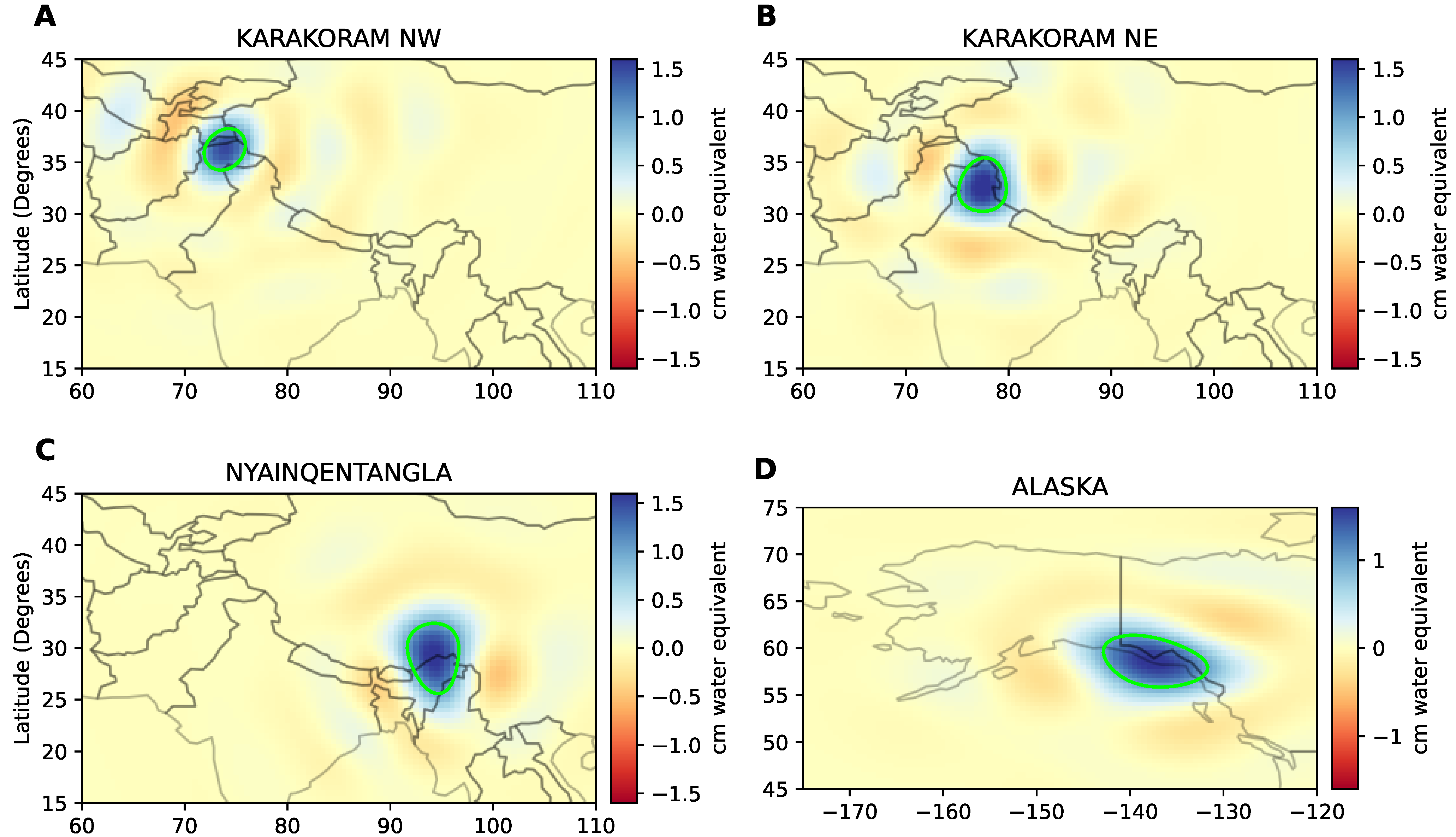
In each case, we find that the optimal mascon configuration is achieved by defining one fixed point for the region of interest, which allows for more flexibility in optimizing the mesh. For the Karakoram, Nyainqentangla, and Alaska, we used a total of 153, 144, and 113 mascons, respectively. These hyperparameters were determined through trial-and-error. The number and size of mascons are important in order to obtain the localized mass change of the region of interest, while keeping the degrees of freedom (i.e., the total number of mascons to be fitted), to a minimum elsewhere. In addition, larger mascons in the far-field minimize the effect of sharp edges and corners due to the truncation of the harmonics. The harmonic representations of the chosen mascons in the region of interest and the far-field for the each configuration are shown in Figure 2.

To understand the area being sampled by the optimized mascon configuration, it is necessary to examine the corresponding sensitivity kernel, given by Equation (A6) of [20]:

$$M_i\left(t\right)=\int \sigma (\theta ,\varphi ,t)A(\theta ,\varphi )R_{earth}^{2}sin\left(\theta \right)d\theta d\varphi$$

(3)

where $M_i\left(t\right)$ is the mass of mascon i at time t, $\sigma (\theta ,\varphi ,t)$ is the actual surface mass density at time t, $A(\theta ,\varphi )$ is the value of the sensitivity kernel at point $(\theta ,\varphi )$, and $R_{earth}$, $\varphi$, and $\theta$ serve as the mean radius of the Earth, longitude, and co-latitude, respectively.

Due to the non-uniform distribution of mass within mascons and the truncated nature of the harmonics, there is inevitably some leakage of the mass balance signal between mascons, and the kernels may not correspond to the expected harmonic representation of the corresponding mascons. This leakage should be included in the uncertainty estimates of the final solution. To do this, we compare the kernels of the mascons of interest, with harmonic representations for the corresponding mascons, such as those shown in Figure 2. In an ideal situation where all mascons are truly orthogonal to each other, the kernels would be exactly equal to 1 inside the kernel and 0 outside, i.e.,

$$\frac{1}{S_j}{\int }_{S_j}{A}_i(\theta ,\varphi )sin\theta d\theta \varphi ={\delta }_{ij}$$

(4)

where $A(\theta ,\varphi )$ is the kernel of mascon i at point $(\theta ,\varphi )$, $S_j$ is the surface area of mascon j, and ${\delta }_{ij}$ is the Kronecker delta function [20].

Any leakage between mascons, which violates the orthogonality assumption, leads to a deviation from Equation (4). Therefore, as a first-order approximation, we quantify this violation as the percentage of mass represented by the kernel outside of the mascons, compared to the mass represented inside the mascons:

$${\delta }_{leakage}=\frac{{\displaystyle \sum _{\begin{array}{c}i=0\\ i\not\subset M\end{array}}^N}\left({\displaystyle \sum _{l,m}^{60,60}}\left[A_{l,m}^{c,M}{C}_{l,m}^i+A_{l,m}^{s,M}{S}_{l,m}^i\right]\right)}{{\displaystyle \sum _{\begin{array}{c}i=0\\ i\subset M\end{array}}^N}\left({\displaystyle \sum _{l,m}^{60,60}}\left[A_{l,m}^{c,M}{C}_{l,m}^i+A_{l,m}^{s,M}{S}_{l,m}^i\right]\right)}\times 100$$

(5)

where N is the total number of mascons, M is the set of mascons of interest, for which the leakage error is calculated as a group (e.g., 2 mascons out of a total of 162 in the case of Karakoram SE and NW), $A_{l,m}^{c,M}$ and $A_{l,m}^{s,M}$ are the cosine and sine harmonic coefficients of the sum of sensitivity kernels for mascons in set M, and $C_{l,m}^i$ and $S_{l,m}^i$ are the Stokes coefficients of mascon i of degree and order 60. Note the sum in the numerator is only for mascons not belonging to set M (i.e., $i\not\subset M$), representing the mass sampled outside the region of interest. The sum in the denominator is only for the complementary set (i.e., $i\subset M$), where the kernel and mascon harmonics correspond to the same region, representing the mass sampled inside the region.

3. Results

Figure 3 shows the sensitivity kernels as described by Equation (3) for mascon combinations in northwest Karakoram (A), southeast Karakoram (B), Nyainqentangla (C), and Alaska (D).

The kernels highlight the fundamental trade-off between the size of the sampled area and the amount of ringing. In order to separate the Karakoram region into physically meaningful regimes, we sample different mascons for the northwestern (NW) and southeastern (SE) regions. The spatial variability of geophysical mass change signals in this area dictates the need for smaller mascons, which inevitably results in a higher amount of ringing due to the truncated nature of GRACE harmonics. With the dynamic mascon tool, the user can make this choice consciously and quantify the amount of leakage. More importantly, the same kernel can be applied to various non-GRACE data, such as hydrological model output, for comparison. Developing custom mascons from Level-2 harmonics provides researchers with the ability to examine the sensitivity kernel of mascon aggregates to quantify any leakage and rigorously sample gridded non-GRACE data within the kernel where the gravimetric data are sampled. Furthermore, non-global mascon configurations such as those of [18] are prone to ringing in the sensitivity kernel at the boundaries of the mascon grid. While this is manageable on the Antarctic Ice Sheet, which is surrounded by the Southern Ocean and has distant sources of far-field contribution to the kernel, it becomes a larger issue in smaller inland areas such as High Mountain Asia. Our automatic global configuration minimizes this problem.

Given the fundamental trade-off between the sampled area and the amount of ringing and leakage, it is crucial to fully quantify the leakage error in the error estimate. This is another advantage of directly working with mascon kernels, where the user can fully account for any leakage from the kernel depending on the area being sampled. We calculate this leakage error following Equation (5). The results for each of the regions represented in Figure 3 are shown in

Table 1. The leakage error for each of the mascon configurations, expressed as mean percent error as in Equation (5).

Region	${\mathit{\delta }}_{\mathit{leakage}}$ (%)
Karakoram (NW)	32.0
Karakoram (SE)	20.3
Nyainqentangla	24.0
Alaksa	31.6

.

4. Discussion

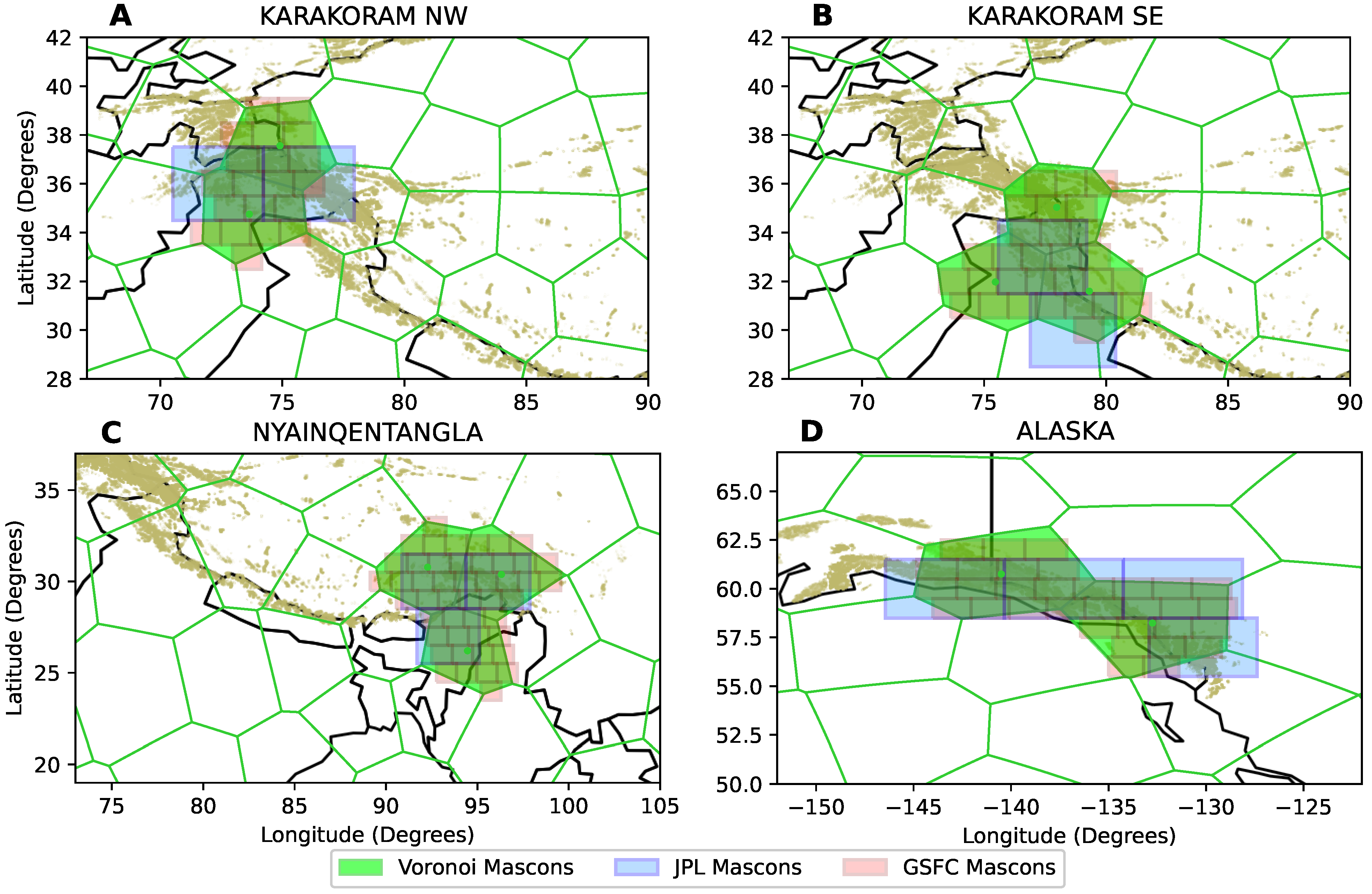
We compare the regional case studies presented in the previous section to the closest corresponding estimates from the JPL and GSFC range-rate mascon solutions. The JPL mascon solutions are provided on a global set of 4551 3${}^{\circ }$ spherical cap mascons [11]. The GSFC solutions are provided on a global set of 41,168 1 × 1 arc-degree mascons [13,14], where regularization constraints are applied over collections of mascons and the sub-resolution mascons are meant to be aggregated for regional estimates. Given that these mascon solutions are fixed and global in nature, they are not tailored towards the regions presented in this study. As a result, we sample the closest overlapping mascons for each region, as presented in Figure 4. Given the Voronoi mascons designed for a particular region, we select the corresponding JPL and GSFC mascons with the condition that at least 50% of the area of a given mascon overlaps with the Voronoi mascons. This further demonstrates the need to develop regionally tailored global solutions, as geophysically distinct regions are unlikely to be sampled in a physically meaningful way at all locations with a fixed uniform global grid. For example, the geophysically distinct regions in the Northwest and Southeast Karakoram are challenging to separate from the larger JPL mascon configuration. While the smaller GSFC mascons allow for the easier separation of regions, analysis of individual mascons can be problematic without examining the associated covariance matrix or sensitivity kernel to minimize leakage. Furthermore, to minimize any oceanic contributions to the mascons in coastal Southeastern Alaska, we apply land masks to both the JPL and GSFC mascons. The Voronoi mascons are derived from GSM GRACE harmonics, which already have the oceanic signal removed. Note that fitting the GSM coefficients to the JPL and GSFC mascon grids in the harmonic domain is not feasible for a few reasons. On a practical level, while fitting 100 Voronoi mascons to the GRACE data can be completed in minutes on a personal computer, fitting thousands to tens of thousands of JPL or GSFC mascons is computationally impractical for most users. Furthermore, the regularization constraints of the JPL and GSFC mascon solutions are not readily available and are outside of the scope of the present study. More fundamentally, however, fitting 3721 harmonics (maximum degree and order 60) to 4551 JPL mascons or 41,168 GSFC mascons is an ill-posed problem without additional information. This illustrates another advantage of our dynamic Voronoi approach, which allows the user to perform a well-posed global regression.

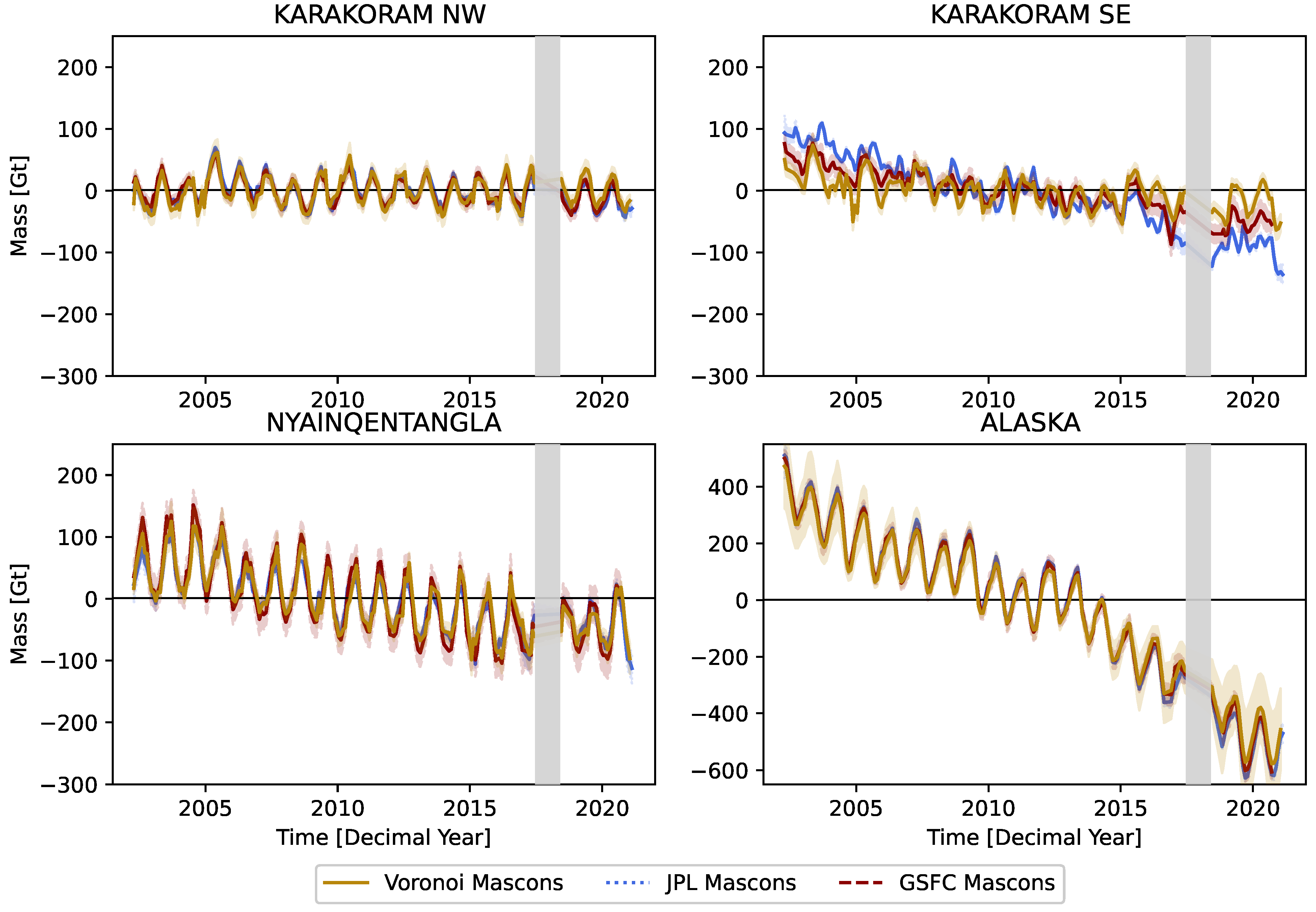
We evaluate the time series from each of the three mascon solutions for the four case-study sites. For consistency, we apply the same JPL and GSFC corrections to the Voronoi mascons, as outlined in Section 2, including the same GIA correction using the ICE6G-D model [36]. The resulting time series are shown in Figure 5. The errors for the Voronoi mascons are derived from the leakage error as shown by Equation (5), added in quadrature with the 1-sigma GRACE measurement error as in [40]. For the JPL and GSFC mascons, we include the uncertainty estimates provided with the solutions. Note that while the JPL solutions provide a 1-sigma uncertainty estimate, the uncertainty estimates provided by the GSFC are 2-sigma. Despite the more conservative error estimates, we observe a few differences between the solutions, although there is excellent overall agreement, as described below.

We find that, overall, there is good agreement between the three mascon solutions in the four sampled areas. This increases confidence that our custom Voronoi mascon methodology correctly samples the mass change time series of the region of interest, while providing more flexibility to the user to directly work with the design of mascons and the associated kernels. However, we also observe notable differences between the solutions. Namely, the JPL and GSFC mascons show larger mass losses in SE Karakoram compared to the custom Voronoi mascons. Specifically, the JPL and GSFC solutions show trends of −9.47 ± 0.40 Gt/yr and −5.70 ± 0.31 Gt/yr, respectively, for the period April 2002 to September 2020. On the other hand, the Voronoi solution exhibits a trend of −2.30 ± 0.37 Gt/yr. The uncertainty estimates are given at the 95% confidence level using the t-distribution. Given the mass loss regions adjacent to SE Karakoram, particularly to the south, as shown by [37], the larger mass loss of the JPL and GSFC solutions may be explained by the less targeted sampling of these solutions. In particular, the larger JPL mascons, which have the lowest trend in our analysis, sample larger areas to the south Figure 4.

In NW Karakoram, we again find that the JPL solutions have the most negative trends, followed by the GSFC and Voronoi solutions. The JPL mascon solution has a trend of −1.04 ± 0.38 Gt/yr for the period from April 2002 to September 2020. The GSFC solution shows a trend of −0.93 ± 0.23 Gt/yr, while the targeted Voronoi solution has a trend of 0.06 ± 0.34 Gt/yr for the same period. While the negative trends of the GSFC and JPL solutions are in agreement within uncertainty, they are not in agreement with the Voronoi solution. The results of [37] suggest that while NW Karakoram showed a slightly positive mass balance in this period, surrounding areas exhibited a negative mass balance, which likely explains the more negative trends shown by the larger JPL mascons. The highly customizable and yet global nature of our Voronoi mascons allows the user to further isolate these geophysically distinct areas. It is important to emphasize that using these solutions to assess the assumptions and methodologies of each product is beyond the scope of this paper. However, the Voronoi mascon approach allows one to more carefully assess the region being sampled on a case-by-case basis, which is not possible with static global solutions.

It is also interesting to examine the differences in the seasonal amplitude between the three solutions. The JPL and GSFC solutions use a priori information to regularize the mascons, minimizing the covariance between groups of mascons. We see that in SE Karakoram, the Voronoi solutions show larger seasonal amplitude and more noise. We find a seasonal regression coefficient (the sum in quadrature of cosine and sine components of the seasonal variability) of 22.5 ± 3.9 Gt for the Voronoi mascons, compared to seasonal amplitudes of 8.2 ± 4.2 Gt and 12.1 ± 3.2 Gt for the JPL and GSFC solutions, respectively, for the period April 2002 to September 2020. Note that the unregularized nature of the Voronoi mascons leads to more noise, whereas regularized solutions may have dampened variability. A careful assessment of seasonal variability in these regions based on auxiliary environmental variables is outside of the scope of this study. In the Nyainqentangla region, we do not find larger seasonal amplitudes for the Voronoi solutions. We find seasonal amplitudes of 45.2 ± 5.2 Gt, 42.0 ± 4.8 Gt, and 58.1 ± 5.1 Gt for the Voronoi, JPL, and GSFC solutions. In coastal Alaska, we find the seasonal amplitudes to be in agreement, with coefficients of 94.0 ± 13.4 Gt, 98.8 ± 17.2 Gt, and 93.5 ± 15.0 Gt for the Voronoi, JPL, and GSFC solutions, respectively. It is important to note that the constraints applied to the GSFC solution occur across the entire Gulf of Alaska [13]. In general, Alaska glaciers along the coast exhibit large seasonal variability due to proximity to maritime conditions, so the constraints may be much more physically realistic than those in the Karakoram, where we see greater spatial variability in seasonal mass balances. It may be less important to have the level of control over mascons provided by the Voronoi methodology in regions with more homogeneous geophysical signals, but it becomes increasingly important where there is more spatial variability.

Previous GRACE studies tend to group larger areas together, or focus on regional configurations that require ad-hoc processing to remove far-field effects (e.g., [41]). The automated global variable-size mascon generation solution described here allows users to further isolate physically meaningful distinct regions, while having direct access to the kernels to minimize and quantify leakage for specific configurations. The L1B Regression Mascons using the “Resolution Operator” by [42] are calculated at an even higher resolution of 1 arc-degree. However, these solutions use the inherent trade-off between the temporal and spatial resolution of GRACE data in order to obtain a high spatial resolution for trends across long timespans. While our dynamic mascon solution is still restricted by the spatial resolution of monthly GRACE data at degree and order 60 or about 330 km, we can provide dense time series data with the same monthly sampling as the standard JPL and GSFC mascon solutions.

5. Conclusions

Gridded mascon products from range-rate data such as those from the JPL [11] or GSFC [13,14] do not give users direct control over the placement of the mascons or the regularization assumptions used during the creation of the solutions. An alternative approach involving manually designed mascons based on Level-2 harmonics for regions of interest, such as those of [17,21], can be arduous and time-consuming to build and suffer from far-field leakage for regions such as High Mountain Asia.

We present an open-source pipeline to produce global mascon solutions based an iterative spherical Voronoi tessellation scheme centered on user-defined point(s) or polygon(s) of interest. The mascons gradually increase in size in the far-field, minimizing the effect of noisy higher degree harmonics and computational cost where high spatial resolution is not needed.

We find that our solutions are in overall agreement with the JPL and GSFC solutions for four case-study sites of NW and NE Karakoram, Nyainqentangla, and SE coastal Alaska. The improved sampling of the Voronoi mascons, however, leads to differences in observed mass change trends. In addition, the different regularization and a priori assumptions may lead to differences in the seasonal variability of the solutions in some locations. While the JPL and GSFC solutions show dampened seasonal variability over SE Karakoram compared to the Voronoi mascon solution, they show a similar or larger seasonal variability in the Nyainqentangla and Alaskan regions.

Previous GRACE analyses in heterogeneous regions such as High Mountain Asia tend to aggregate large regions, rely on ad-hoc processing to remove far-field effects from regional configurations [41,43], and/or sacrifice temporal resolution for higher spatial resolution [42]. Our automated approach allows users to easily and quickly experiment with global configurations of variable area mascons to isolate the mass change for relatively small, physically distinct regions (subject the resolution of GRACE at degree and order 60) with a monthly resolution. Our approach also offers direct access to the underlying kernel, which can also be used to sample non-GRACE data for comparison and analysis and to quantify leakage. In addition to the configuration and placement of the mascons, the user also has control of the assumptions and corrections that are used in the processing, which can be tailored to meet the goals of the study. While we tested our methodology for four different regions, future studies can deploy the same pipeline for various hydrological or glaciological basins across the globe.