Assessment of Empirical Algorithms for Shallow Water Bathymetry Using Multi-Spectral Imagery of Pearl River Delta Coast, China

Abstract

Pearl River Delta (PRD), as one of the most densely populated regions in the world, is facing both natural changes (e.g., sea level rise) and human-induced changes (e.g., dredging for navigation and land reclamation). Bathymetric information is thus important for the protection and management of the estuarine environment, but little effort has been made to comprehensively evaluate the performance of different methods and datasets. In this study, two linear regression models—the linear band model and the log-transformed band ratio model, and two non-linear regression models—the support vector regression model and the random forest regression model—were applied to Landsat 8 (L8) and Sentinel-2 (S2) imagery for bathymetry mapping in 2019 and 2020. Results suggested that a priori area clustering based on spectral features using the K-means algorithm improved estimation accuracy. The random forest regression model performed best, and the three-band combinations outperformed two-band combinations in all models. When the non-linear models were applied with three-band combination (red, green, blue) to L8 and S2 imagery, the Root Mean Square Error (Mean Absolute Error) decreased by 23.10% (35.53%), and the coefficient of determination (Kling-Gupta efficiency) increased by 0.08 (0.09) on average, compared to those using the linear regression models. Despite the differences in spatial resolution and band wavelength, L8 and S2 performed similarly in bathymetry estimation. This study quantified the relative performance of different models and may shed light on the potential combination of multiple data sources for more timely and accurate bathymetry mapping.

1. Introduction

70% of the Earth’s surface is covered by ocean, and the total length of global coastlines is more than 1.16 million kilometers [1]. Nearshore bathymetry is critical to monitoring nearshore activities, such as port facility management, fishing, movement of deposited sediments and pipeline laying [2,3]. Timely and accurate bathymetric information is also necessary to support effective resource policy making and management for coastal environment, as well as to assure human safety and welfare [4].

Bathymetry is traditionally mapped via in situ measurements, such as vessel-based acoustic echo sounding, to generate accurate point measurements or depth profiles along transects [5]. However, the echo sounder survey is constrained by its time-consuming nature and the high operational cost [6]. In addition, due to the swath angle and the distance between the survey vessel and shore, the survey system will result in a blind area on the shore terrain outside the swath coverage [7]. As a result, the echo sounder survey cannot be applied in the shallow waters with complex underwater terrain. Remote sensing techniques are able to derive nearshore bathymetry over varying spatial and temporal scales efficiently and repeatedly over large areas. Satellite-derived bathymetry (SDB) are generally divided into two broad categories: the microwave imagery-based methods and the multi-spectral imagery-based methods [2]. The microwave imagery-based methods use radar backscatters to capture variations of sea surface velocity and estimate water depth through the interactions between tidal flow and sea bottom topography. The accuracy of this method is heavily influenced by wind speed, and is vulnerable to the speckle-infested radar imagery [8].

Unlike microwave remote sensing, the principle of optical bathymetry mapping is to determine water depth using the total amount of radiative energy reflected by the water column [9]. The spectral bands of optical satellite imagery (e.g., blue and green bands) normally feature strong penetration capacity through clear water. With higher concentration of suspended sediments in the water body the reflection peak of the water body shifts to longer wavelength [10,11]. As the incident solar radiation propagates through water, it is partly scattered and absorbed by water and in-water constituents, and partly backscattered and recorded by multi-spectral sensors. Multi-spectral imagery thus enables the production of finer resolution bathymetric information than the microwave-based methods, though the range of detectable depth is reduced [12,13].

The commonly used optical bathymetry mapping algorithms mainly consist of analytical models and empirical models [2,14]. The analytical models adopt the flow radiative transfer models that take the sunlight and atmospheric variations into consideration. Since such models are constrained by single band information, they are not applicable to areas with variant optical properties and bottom reflectance [15,16,17]. In the empirical approaches, multi-spectral bands are combined to establish linear/non-linear regression models between remotely sensed radiance of the water body and the observed water depth [18,19]. Compared with analytical models, empirical models are able to account for the water conditions (e.g., water clarity, bottom reflectance) as well as the atmospheric conditions (e.g., atmospheric absorption and scattering effect) in a more efficient way [20,21].

However, it is worth noting that the accuracy of optical bathymetry is subject to influence from the spatial, spectral and radiometric resolution. Medium resolution satellite data (e.g., Landsat TM, Landsat 8) and high resolution satellite data (e.g., SPOT, RapidEye) have been applied in previous bathymetry studies, and have achieved different accuracies [22,23,24]. Finer spatial resolution does not guarantee higher accuracy in bathymetry retrieval. Instead, the radiometric resolution of selected spectral bands as well as the water turbidity are at least as important as the spatial resolution in affecting the accuracy of bathymetry retrieval [25,26]. In particular, water tides, waves, sea floor materials and water clarity exert impacts on the reflected radiation. It is thus imperative to integrate different levels of water depth samples with different spectral bands to explore the influence of water conditions on bathymetry retrievals [27,28,29].

Sentinel-2 (S2) imagery, with a 5-day revisit, 10 m multi-spectral resolution, offers a new source of freely available dataset in bathymetry retrieval. The imaging swath of S2 data is 290 km wide, much wider than that of Landsat 8 (L8) and WorldView-2 [30]. It thus has the advantage of a wider range of view angles and facilities a larger simultaneously mapped area [31]. Preliminary results have suggested that S2 satellite data are potentially useful for mapping inland water quality, coral reefs, as well as bottom depth with varied degrees of success [30,32,33]. While the mixed resolution of optical spectral bands (e.g., 60 m for the equivalent of the deep blue band from L8) in S2 satellite still calls for further evaluation of its capability in bathymetry mapping [34,35].

With the advantages in spatial coverage, revisit frequency and availability, L8 and S2 have been individually explored in SDB in many previous studies. However, their spectral discrepancy as well as their capacity in retrieving bathymetry over large areas of shallow water at different time periods have not been explicitly evaluated. In this study, we incorporated multi-spectral information from L8 and S2 data to derive bathymetry in a large coastal region of the Pearl River Delta (PRD), China from 2019 to 2020 with Google Earth Engine (GEE). Four widely used empirical models, namely the linear band model [36], the log-transformed band ratio model [23], the support vector regression model [37] and the random forest regression model [38] were adopted. To evaluate model performance with areal spectral features, all models were applied both with and without area segmentation. It is the first study for satellite-derived bathymetry near the PRD coast (over 3000 km²) validated with a large volume of validation data (over 600 ground samples). The novelty of this study lies in the comprehensive comparison of the bathymetry estimation based on two satellite products, in which different pre-processing steps, multispectral band combinations and spatial regression techniques were investigated. A thorough understanding of the strengths and weaknesses of the L8 and S2 data in bathymetry mapping, as well as the relative performance of different methods will facilitate bathymetry estimation under different environmental conditions and may serve as a reference for the potential combined use of both data sets for higher resolution, more timely bathymetry mapping.

2. Study Area and Data

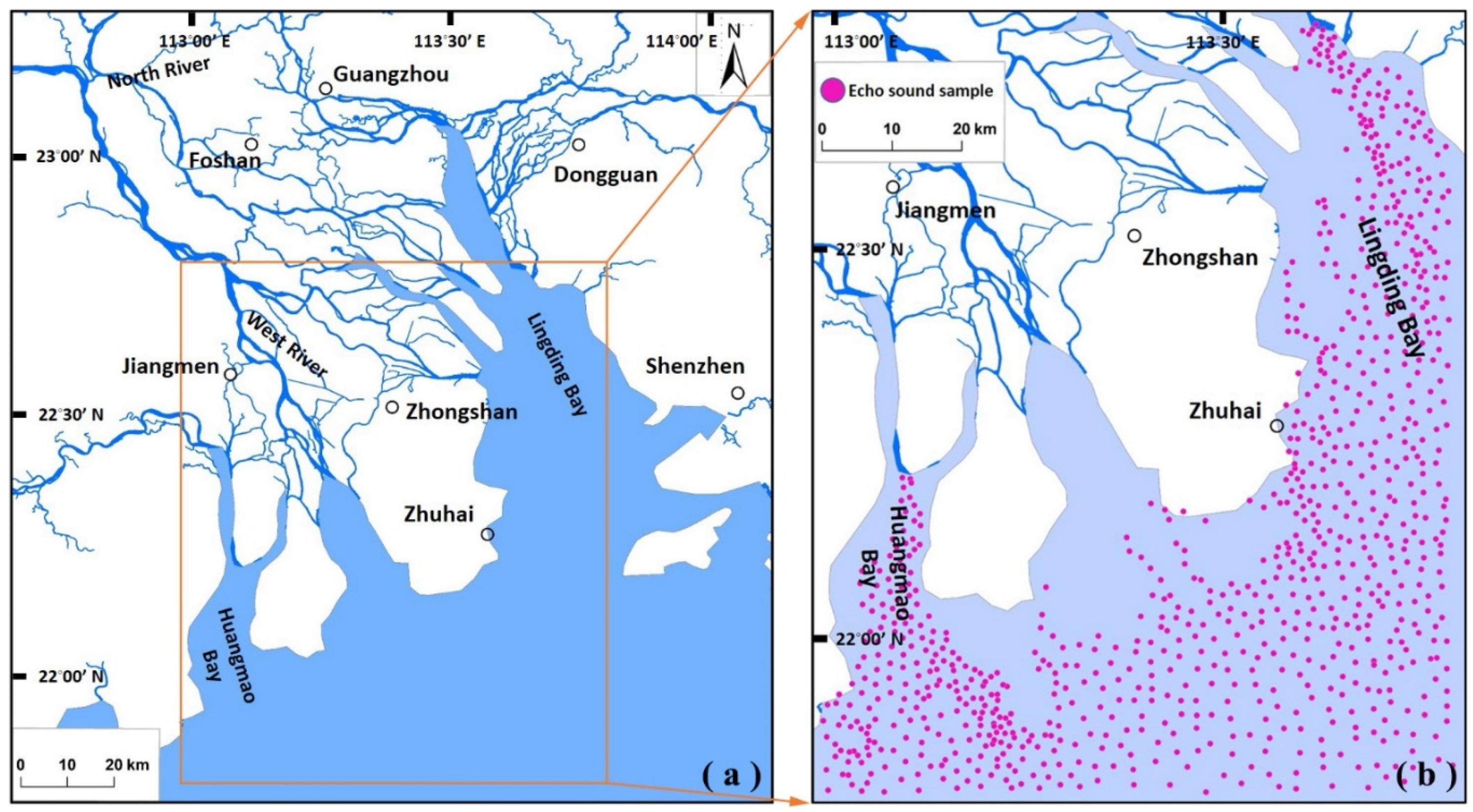
2.1. Study Area

The Pearl River, as one of the 25 largest rivers in the world and the third-largest river in China, extends from 21°N to 24°N, 112°E to 115°E. The study area (Figure 1) covers the Lingding Bay and the Huangmao Bay, which are the two biggest sub-estuaries of the PRD. The region features a subtropical climate, and the annual precipitation varies between 1500 and 2000 mm. The Pearl River receives discharge and sediment from the West River, the North River and the East River. In recent years, intensive human activities, such as aquaculture and human-induced land use and land cover change, have dramatically changed the morphology and altered the hydrodynamics [39]. For example, the average water depth increased from 4.2 to 4.6 m between 1980 to 2010 due to decreasing sediment input from dam construction in the Lingding Bay, and the mean tidal range is amplified from 1.1 m near the mouth to 3.7 m near the top of the bay [38].

2.2. In Situ Bathymetry Data

In-situ bathymetry data were obtained from the China Navy Hydrographic Office (CNHO), which is China’s official hydrographic surveying and mapping organization and the only publishing house for nautical publications authorized by the government. The CNHO performs periodic surveys using echo sounding equipment in the coastal areas for the purpose of maritime safety, marine route monitoring and management for the coastal spatial planning and environmental protection. A total of 667 in situ survey samples were acquired between 2017 and 2020 using a 5-m inflatable boat equipped with a Lawrence High-Definition System (HDS).

2.3. Satellite Data and Pre-Processing

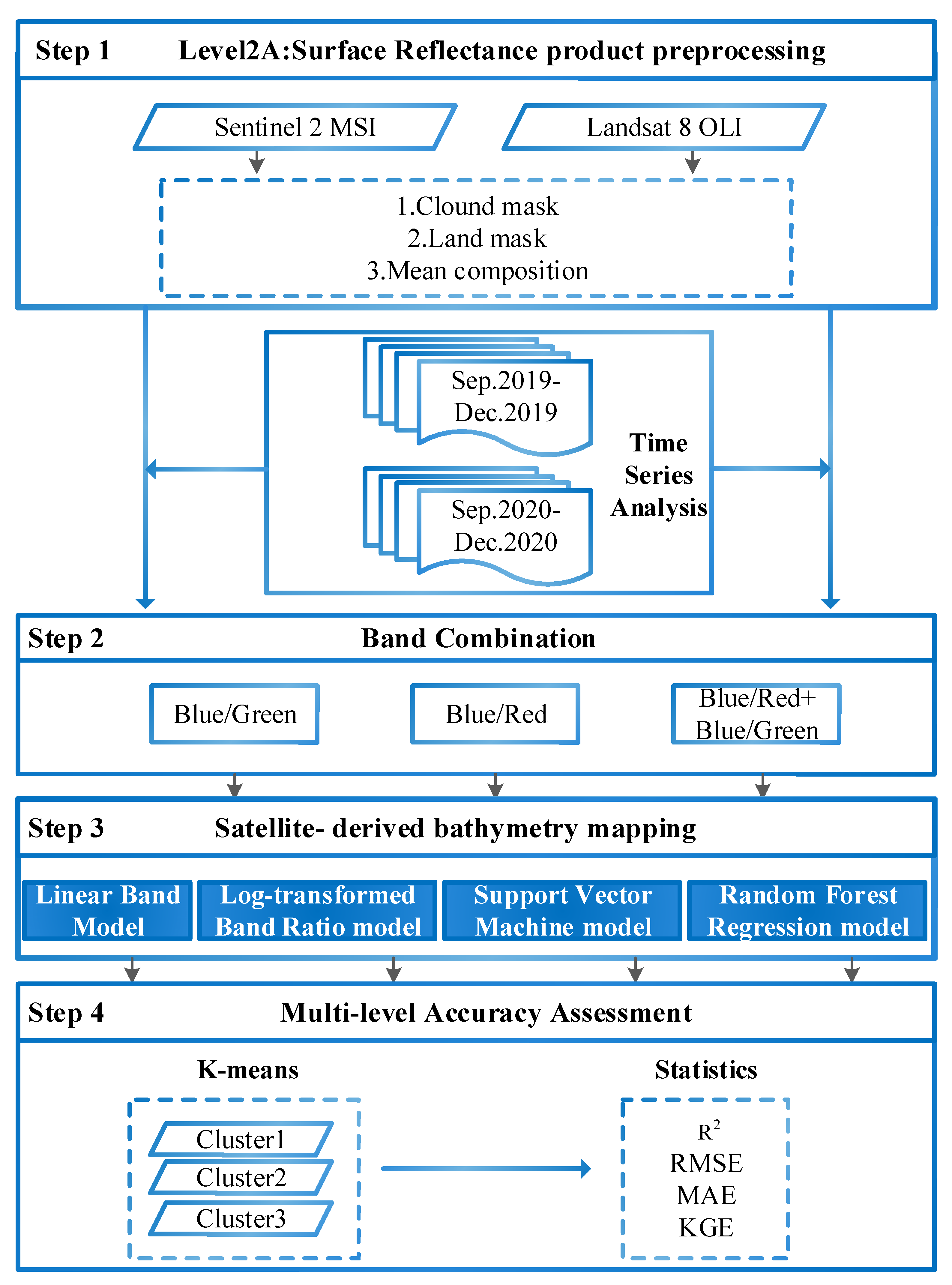
The cloud cover and water column conditions hampered the amount of suitable satellite images along the Pearl River coast. Therefore, only the surface reflectance data of L8 and S2 with cloud coverage lower than 20% from September to November in 2019 and 2020 were used in the analysis. As GEE is a cloud-based geospatial computing platform that offers a petabyte-scale archive of freely available S2 and L8 imagery, we averaged the three months’ images in each year to generate a new image collection for subsequent analysis. All these surface reflectance data of L8 and S2 were masked for clouds and land areas in GEE. The details of the datasets are summarized in

Table 1. Details of satellite data used in this study.

	L8	S2
Swath width	185 km	290 km
Spatial resolution	30 m	10 m
Revisit interval	8 days	5 days
Temporal coverage	11/02/2013–present	23/06/2015–present
Spectral bands used	Red (636–673 nm)	Red (664.5–665 nm)
	Green (533–590 nm)	Green (559–560 nm)
	Blue (452–512 nm)	Blue (492.1–496.6 nm)
Image volume processed	8 images (2019)	46 images (2019)
	8 images (2020)	26 images (2020)

.

3. Methodology

The methodology is illustrated in Figure 2. Four models based on light attenuation in the optical bands were used, namely the Linear Band Model, the Log-transformed Band Ratio Model, the Support Vector Regression Model and the Random Forest Regression Model. Considering the data availability and cloud contamination of the optical data, the mean composite images acquired in autumn (September to November) in 2019 and 2020 were extracted.

To maximize the water depth that can be derived by satellite measurements, spectral bands with the lowest level of radiation absorption (i.e., Red, Green and Blue bands) were combined to derive water depth [23,39,40]. Before applying the models, the K-means clustering algorithm was applied to segment the study area into multiple clusters based on the spectral features. We assumed that clustering enables better interpretation of the relationship between water depth and multi-spectral characteristics and reduces the bias as well as uncertainty of bathymetry estimation over a wide variety of bottom types. All models were also applied without a priori K-means clustering for comparison. The estimation uncertainties were quantified by comparing the satellite-derived and surveyed bathymetry across different clusters separately.

3.1. K-Means Clustering

The K-means clustering algorithm makes use of the spectral similarity of the image to perform dimensionality reduction. It segments the image into k clusters. Each pixel has a degree of membership in cluster i, and the degree of membership in each pixel is achieved by computing the relative distance between the pixels and cluster centroids. In this study, we used K-means to reduce the bias and errors that may occur in the bathymetry estimation.

The number of clusters needs to be given to the K-means algorithm as an input. After trial and error, we segmented the images into three clusters in this study, as the image would be too fragmented when the choice of k was larger than three. The average water depth in each cluster ranged from 3.18 m to 12.88 m in 2019 and from 2.13 m to 13.05 m respectively in 2020 for S2 images and ranged from 4.14 m to 16.06 m in 2019 and from 5.40 m to15.23 m in 2020 for L8 images (details are shown in Table S1 in the supplementary materials).

3.2. Linear Band Model (LBM)

The linear band model was proposed by Lyzenga et al. [36] for calculating water depth from satellite imagery based on the Beer-Lambert law of absorption (Equation (1)). This model assumes a linear relationship between the log-transformed band reflectance and water depth via multiple linear regression:

$$h_j=h_0+h_1\ln \left(R_j-R_{wj}\right)$$

(1)

where $h_j$ is the water depth derived from band j, $R_j$ is the surface reflectance in band j, and $R_{wj}$ is the average reflectance of deep water. Nevertheless, depth-independent variability in reflectance between bands and factors such as water quality heterogeneity all contribute to errors in the depth estimated using Equation (1). Lyzenga et al. [12] used a set of depth-independent variables in Equation (2) to account for volume scattering in the water column and external water reflection, including sun glint effects and atmospheric scattering:

$$D_i=h_0+{{\displaystyle \sum }}_{j=1}^N{A}_{i,j}{h}_j$$

(2)

where $A_{i,j}$ is the $i^{th}$ variable in the rotational matrix for band j. $h_0$ and $h_1$ to $h_j$ are determined through multiple linear regression between a set of known depths and the log-transformed reflectance values at those depths. The reflectance values were log-transformed to calibrate a linear relationship between input reflectance and depth. In this study, to be consistent in our comparison with the existing SDB literature, we exploited two band combinations (i.e., Blue + Green and Blue + Green + Red) in the estimation due to their water penetration capacity.

3.3. Log-Transformed Band Ratio Model (BRM)

The LBM assumes that the water mass is homogenous across the study area [23]. However, in turbid waters, especially under conditions with suspended sediments, the assumption is often violated. Consequently the depth estimates under certain benthic environments may be biased [39,41]. The log-transformed band ratio model was proposed by Stumpf et al. [23]. This model assumes that the reflectance in the low-absorption bands decreases more slowly with water depth compared to the high-absorption bands. As a result, the ratio of a high-absorption band to a low absorption band would display a linear decrease with depth when both are log-transformed. As shown in Equation (3), the log-transform reflectance is used to fit a linear relationship between water depth and spectral information to account for water turbidity:

$$h=h_0+h_1\frac{\ln R\left(b1\right)}{\ln R\left(b2\right)}$$

(3)

where h is the satellite derived bathymetry depth, $h_0$ and $h_1$ are fitted parameters controlling the intercept and the slope of the relationship, and $b1$ and $b2$ indicate high-absorption and low-absorption bands (Blue, Green or Red in this study), respectively. The BRM algorithm was implemented using three different band combinations (Blue/Green, Blue/Red and Blue/Green + Blue/Red) to explore the uncertainty of band combination in bathymetry estimation under different water turbidity conditions.

3.4. Non-Linear Regression Model

Machine learning approaches, such as the support vector regression (SVR) model and the random forest regression (RFR) model, serve as alternatives to the standard linear-regression and band-ratio methods to characterize the nonlinear relationship between the spectral information and water depth [42]. Similar to the LBM model, three band combinations (i.e., Blue/Green, Blue/Red, and Blue/Green + Blue/Red) of S2 and L8 were used as predictors for SVR and RFR training, respectively. For the SVR model, the three different spectral band combinations were used to create a high-dimensional feature space, then a radial basis function kernel was implemented to construct a regression hyper plane in this high-dimension space with cross validation [9,18]. For the RFR model, the band combinations were used as the predictors and the water depth was used as the dependent variable, and then the ensemble learning method that combined predictions from multiple random trees were used to generate a more accurate prediction of bathymetry [24,42].

3.5. Accuracy Assessment

To avoid overfitting, we divided the ground samples (667 depth sounding points in Figure 1b) into two sub-datasets (70% for model training, 30% for validation). The coefficient of determination (R²), the Root Mean Square Error (RMSE), and the Mean Absolute Error (MAE) were used to evaluate the bathymetry estimation. The metrics are calculated by

$$R^2=1-\frac{{{\displaystyle \sum }}_{i=1}^n{\left(D_{SDBi}-D_{BFi}\right)}^2}{{{\displaystyle \sum }}_{i=1}^n{\left(D_{BFi}-\overline{D_{BF}}\right)}^2}$$

(4)

$$\mathrm{RMSE}=\sqrt{\frac{1}{n}{\displaystyle \sum }_{i=1}^n{\left(D_{SDBi}-D_{BFi}\right)}^2}$$

(5)

$$\mathrm{MAE}=\frac{1}{n}{\displaystyle \sum }_{i=1}^{\mathrm{n}}\left|D_{SDBi}-D_{BFi}\right|$$

(6)

where $D_{SDB}$ is the depth derived by satellite data, n is the number the validation points, $D_{BF}$ is the field points depth and $\overline{D_{BF}}$ is the mean value. In addition, the Kling-Gupta efficiency (KGE), which measures the mean and distribution of estimates relative to the observations, was also adopted. KGE ranges from negative infinity to unity. The closer KGE is to unity, the better the model performs.

$$\mathrm{KGE}=1-\sqrt{{\left(R-1\right)}^2+{(\frac{{\mu }_E}{{\mu }_o}-1)}^2+{\left(\frac{{\sigma }_E}{{\sigma }_o}-1\right)}^2}$$

(7)

where ${\mu }_E$ and ${\mu }_o$ are the mean values of the simulations and observations, ${\sigma }_E$ and ${\sigma }_o$ are the respective standard deviations.

4. Results

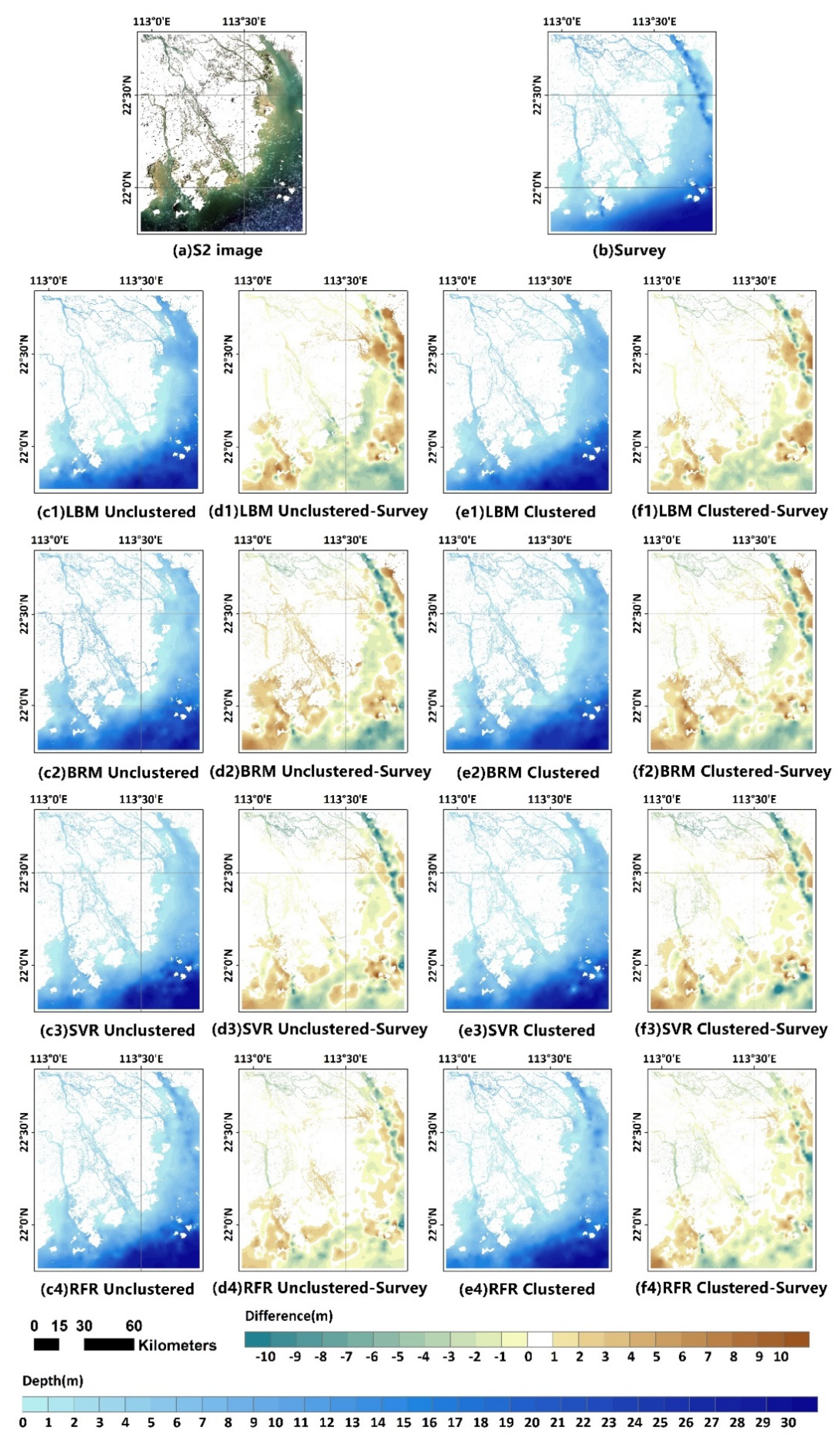
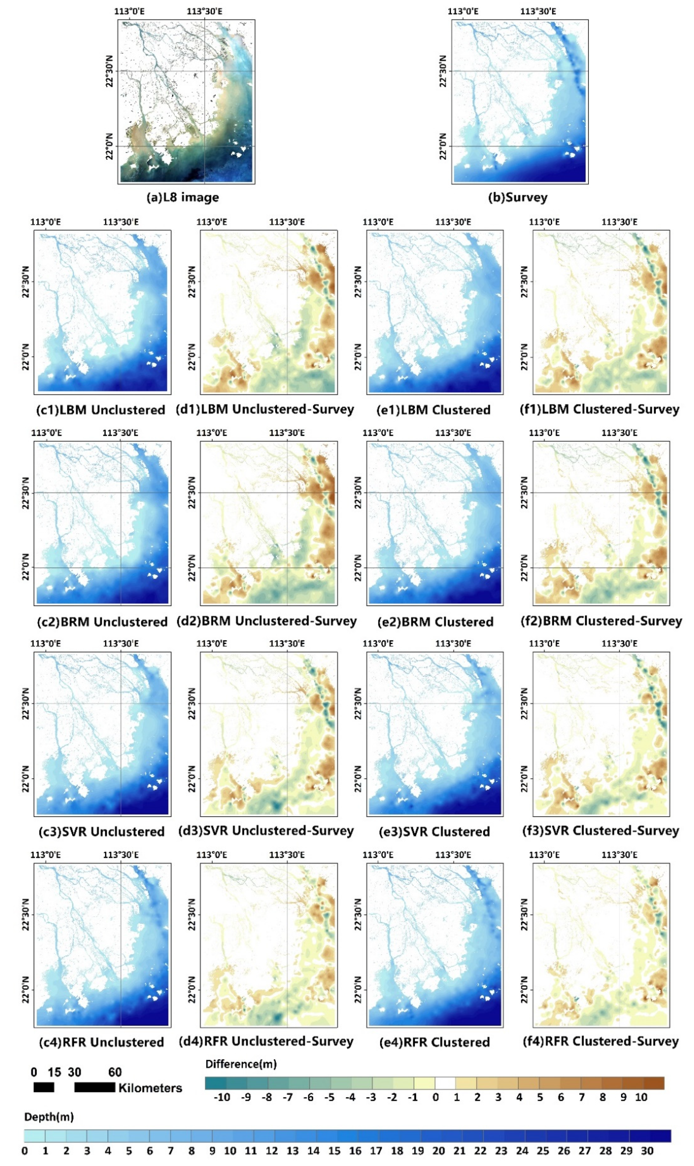
4.1. Bathymetry Estimates with/without Clustering

The SDB estimates with and without clustering from L8 and S2 satellite imagery in 2019 and 2020 using the four approaches considering different band combinations (e.g., B/G, B/R, B + G + R or B/G + B/R) are shown in

Table 2. Statistical metrics of bathymetry mapping for 2019. The units for RMSE and MAE are m. The best performance for each model is highlighted in bold.

2019.9–2019.11			Landsat 8				Sentinel-2
Model	Clustering	Bands	R2	RMSE	MAE	KGE	R2	RMSE	MAE	KGE
LBM	Y	B + G	0.85	3.21	2.40	0.88	0.76	3.77	2.85	0.83
		B + R + G	0.85	3.18	2.38	0.88	0.76	3.75	2.84	0.83
	N	B + G	0.79	3.67	2.96	0.84	0.74	4.08	3.11	0.80
		B + R + G	0.80	3.63	2.92	0.85	0.74	4.13	3.22	0.80
BRM	Y	B/G	0.84	3.24	2.41	0.60	0.77	3.74	2.77	0.83
		B/R	0.82	3.46	2.51	0.70	0.59	4.96	3.72	0.69
		B/G + B/R	0.85	3.21	2.39	0.66	0.78	3.65	2.63	0.84
	N	B/G	0.76	3.92	3.10	0.84	0.71	4.29	3.25	0.80
		B/R	0.67	4.60	3.79	0.77	0.47	5.84	4.50	0.59
		B/G + B/R	0.77	3.89	3.12	0.85	0.75	4.04	3.03	0.82
SVR	Y	B/G	0.85	3.22	2.25	0.92	0.79	3.54	2.30	0.83
		B/R	0.83	3.41	2.37	0.88	0.65	4.55	3.00	0.69
		B/G + B/R	0.86	3.01	1.95	0.92	0.78	3.64	2.28	0.84
	N	B/G	0.79	3.53	2.75	0.87	0.76	3.57	2.38	0.86
		B/R	0.79	3.55	2.62	0.87	0.62	4.48	2.92	0.64
		B/G + B/R	0.80	3.48	2.64	0.90	0.77	3.48	2.32	0.89
RFR	Y	B/G	0.92	2.39	1.54	0.95	0.88	2.70	1.83	0.89
		B/R	0.91	2.46	1.67	0.94	0.80	3.46	2.38	0.84
		B/G + B/R	0.92	2.27	1.45	0.95	0.91	2.35	1.54	0.91
	N	B/G	0.73	4.03	3.01	0.90	0.74	3.68	2.50	0.90
		B/R	0.77	3.71	2.75	0.89	0.52	5.03	3.53	0.79
		B/G + B/R	0.77	3.73	2.73	0.91	0.76	3.55	2.43	0.91

and

Table 3. Statistical metrics of bathymetry mapping for 2020. The units for RMSE and MAE are m. The best performance for each model is highlighted in bold.

2020.9–2020.11			Landsat 8				Sentinel-2
Model	Clustering	Bands	R2	RMSE	MAE	KGE	R2	RMSE	MAE	KGE
LBM	Y	B + G	0.72	4.40	3.39	0.78	0.73	4.23	3.31	0.80
		B + R + G	0.74	4.26	3.32	0.79	0.77	3.89	2.98	0.83
	N	B/G	0.54	5.42	4.38	0.68	0.70	4.41	3.51	0.79
		B + R + G	0.60	5.07	4.16	0.68	0.72	4.22	3.31	0.81
BRM	Y	B/G	0.73	4.33	3.29	0.60	0.72	4.32	3.44	0.79
		B/R	0.62	5.18	4.08	0.70	0.50	5.77	4.65	0.60
		B/G + B/R	0.76	4.14	3.28	0.66	0.77	3.86	2.95	0.83
	N	B/G	−0.15	8.59	6.06	0.33	0.67	4.60	3.75	0.77
		B/R	0.56	5.29	4.13	0.70	0.43	6.04	4.68	0.57
		B/G + B/R	0.44	6.03	4.32	0.72	0.72	4.23	3.49	0.80
SVR	Y	B/G	0.75	4.15	2.94	0.85	0.75	4.11	2.89	0.79
		B/R	0.64	5.06	3.75	0.69	0.51	5.72	4.04	0.59
		B/G + B/R	0.81	3.64	2.66	0.86	0.76	3.96	2.77	0.82
	N	B/G	0.30	6.70	5.19	0.28	0.70	4.14	2.98	0.81
		B/R	0.61	4.99	3.76	0.70	0.46	5.50	4.06	0.62
		B/G + B/R	0.80	3.60	2.76	0.85	0.73	3.89	2.68	0.62
RFR	Y	B/G	0.86	3.08	2.18	0.90	0.87	2.98	2.13	0.88
		B/R	0.78	3.91	2.75	0.82	0.70	4.43	3.08	0.77
		B/G + B/R	0.91	2.44	1.70	0.93	0.91	2.49	1.66	0.90
	N	B/G	0.17	7.30	5.51	0.56	0.71	4.08	3.02	0.88
		B/R	0.58	5.17	3.89	0.78	0.40	5.84	4.24	0.75
		B/G + B/R	0.79	3.70	2.84	0.89	0.76	3.66	2.63	0.91

. The clustering-based SDB estimation outperformed the no-clustering ones in both 2019 and 2020. In details, using the L8 data, the RMSE and MAE decreased by 20.80% and 24.27% on average, and the R² and KGE increased by 0.11 and 0.15 on average with clustering compared with the no-clustering results. Similarly, compared with the no-clustering results using S2 data, the RMSE and MAE decreased by 10.41% and 11.21% on average, and the R² and KGE increased by 0.14 and 0.03 on average when clustering was performed.

The estimation using three bands (i.e., B + G + R or B/G + B/R) outperformed all the two-band combinations in SDB in both 2019 and 2020, with or without a priori clustering. With a priori clustering, the RMSE using three-band combinations ranged from 2.27 m to 3.21 m for L8 and from 2.35 m to 3.64 m for S2 in 2019, and the MAE ranged from 1.45 m to 2.39 m for L8 and from 1.54 m to 2.63 m for S2. The correlations with observations were significant across all SDB models, with R² ranging from 0.92 to 0.85 for L8 and from 0.91 to 0.78 for S2. The KGE metric was also high, which ranged from 0.66 to 0.95 for L8 and from 0.83 to 0.91 for S2. The statistical metrics in 2020 were similar to those in 2019.

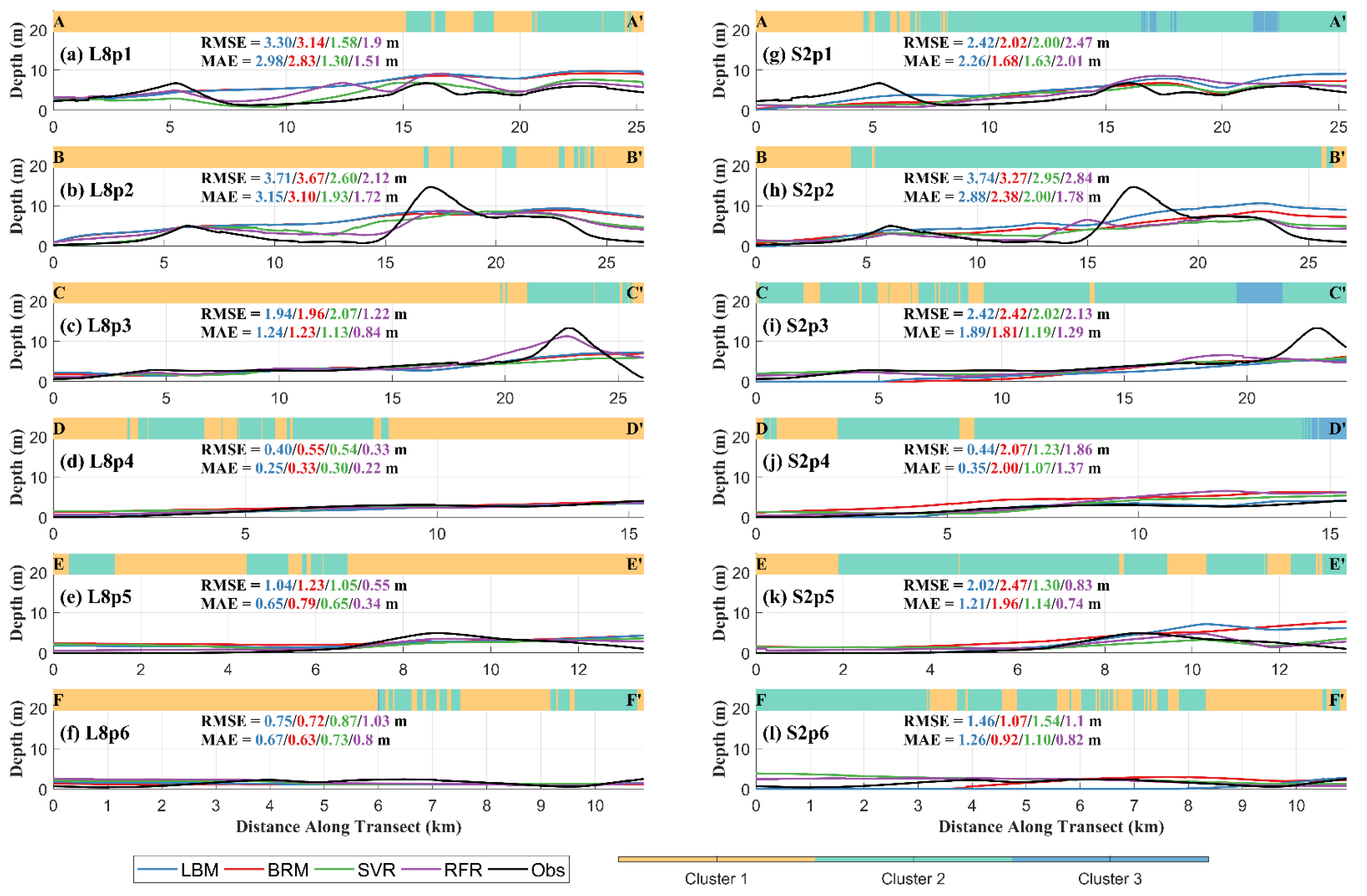
4.2. Bathymetry Estimates in Different Clusters

To evaluate the model performance for water with different spectral features, the SDB estimation results were further compared among different clusters (Figure 3). Similar to the results without clustering (Table 2 and Table 3), the three-band combinations (B + G + R or B/G + B/R) also outperformed all the two-band combinations in the three clusters (included in Tables S2 and S3 in the supplementary materials). Meanwhile, with a priori clustering for L8 images, the non-linear SVR and RVR models performed better than the LBM and BRM models with an average decrease of 11.37% (45.74%) in RMSE and 23.26% (37.33%) in MAE, as well as an increase of 0.02 (0.12) in R² and 0.11 (0.14) in KGE in 2019 (2020), compared to the LBM and BRM models. Similarly, with a priori clustering for S2 images, the non-linear SVR and RVR models also performed better than the LBM and BRM models with an average decrease of 19.59% (15.71%) in RMSE and 36.76% (30.70%) in MAE, as well as an increase of 0.05 (0.06) in R² and 0.07 (0.11) in KGE in 2019 (2020), compared to the LBM and BRM models.

In addition, the largest estimation errors tended to occur in the same areas for all models using S2 and L8 data in 2019 (Figure 4 and Figure 5) and 2020 (included in Figures S1 and S2 in the supplementary material). Specifically, most of the large retrieval differences (>±3 m) were found in areas with depth up to 20 m in the northeast and southwest of the PRD coast. In contrast, to the southeast of the PRD coast where the water is mostly deeper than 25 m, most of the estimation difference is small (<±1 m). Meanwhile, the SDB estimates were closer to the surveyed water depth when clustering was performed a priori. For example, many areas exhibited a large estimation difference with surveyed data (>±3 m) in Figure 4d1–d4 and Figure 5d1–d4 without area clustering, which were reduced to smaller areas with area clustering in Figure 4f1–f4 and Figure 5f1–f4, respectively.

5. Discussion

5.1. Performance of Different Estimation Strategies

For a four-band multi-spectral satellite image (e.g., S2 with 10 m resolution, L8 with 30 m resolution), there are more than 20 possible combinations of optical band ratios or bands [33,43], the determination of the most effective band combination is thus crucial for SDB estimation [30]. In this study, multi-spectral bands which can effectively penetrate the water column were combined (e.g., B/G, B/R, B + G + R or B/G + B/R) and utilized. Their capabilities in retrieving water and underwater reflectance were evaluated based on different empirical retrieval models. The near infrared bands, which cannot effectively penetrate the water column, were not considered. Our results show that the three-band combinations (B + G + R or B/G + B/R) always outperform all the two-band combinations despite of the data sets used. With the four regression models, L8 and S2 demonstrated similar capacities in bathymetry mapping. For example, the linear regression models (i.e., LBM, BRM) using S2 images showed smaller and more consistent prediction difference (lower RMSE and MAE, higher R² and KGE) compared to models using L8 images. In contrast, non-linear regression models (i.e., SVR, RFR) tended to work better for L8 images than for S2 images, with the R² and KGE increased by 0.06 and 0.11 respectively on average and the RMSE and MAE decreased by 10.91% and 3.61% respectively on average.

Meanwhile, when we applied the LBM model to S2 images, the spectral parameters of deep water were obtained from L8 images due to the data availability of S2 images. These parameters performed well for the S2 data, suggesting that the combined use of S2 and L8 information does not introduce large estimation errors.

In addition, it should be noted that the swath of S2 (290 km) is wider than that of L8 (185 km) with some variation in the view angle [30,44]. This offers S2 the capacity to observe a larger area simultaneously compared to L8, which can be particularly advantageous over large coastal regions. The 10 m resolution further enables S2 to better depict benthic features, such as sand, rock, or the coral structure at finer scales than L8. Finally, the short revisit interval (5-day revisit) provided by the S2A and S2B twin satellites provides potential for the evaluation of short-term bathymetry variations.

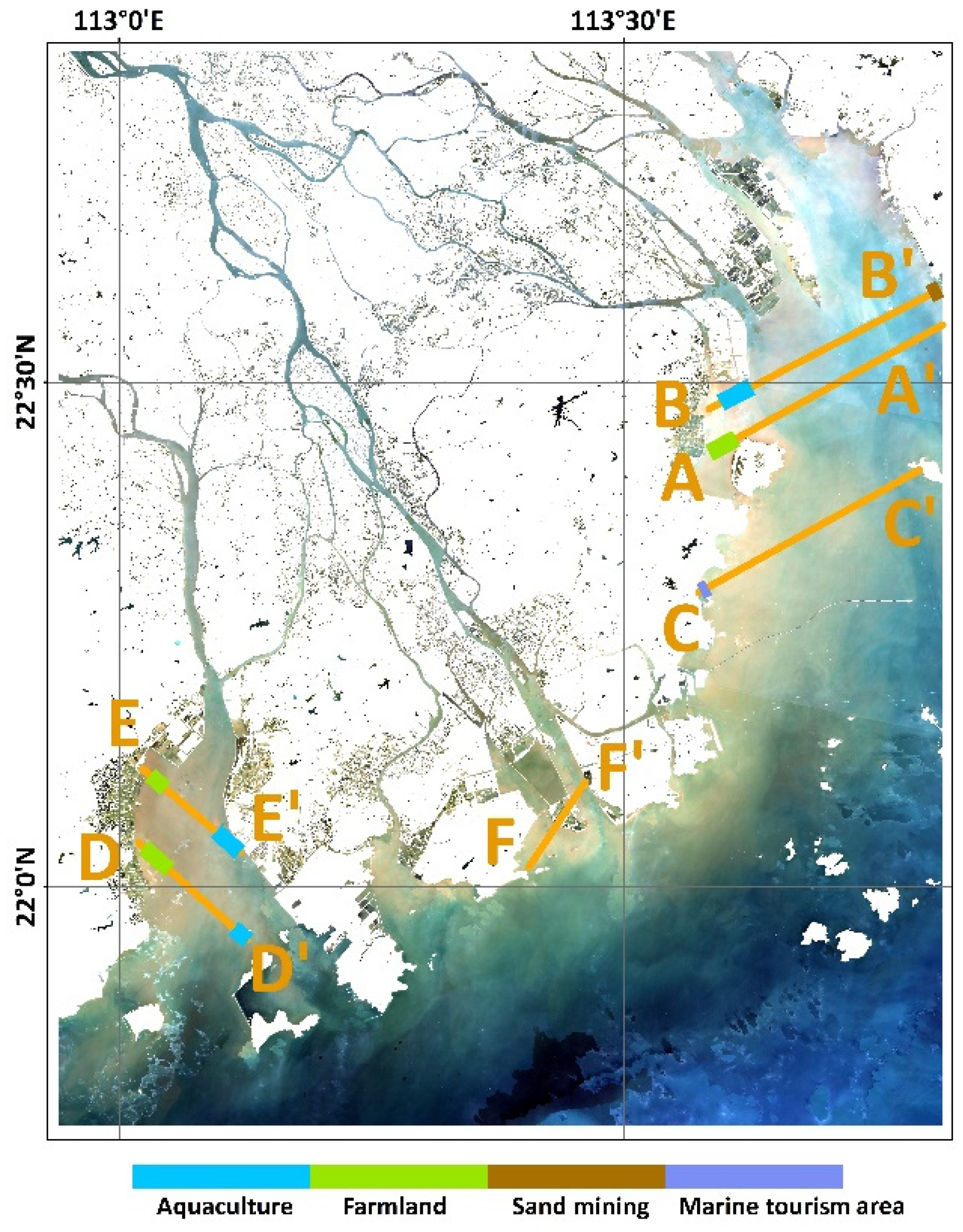
5.2. Influential Factors on the Spectral Information

In order to evaluate the influence of water clarity on the model performance, bathymetrical data were extracted from six transects to compare the performance of the four models under different bottom conditions (Figure 6). The transect lengths range from 10 km to 28 km, with the surveyed depth up to 15 m. The transects span across typical coastal land use types such as aquaculture areas, farmland, tourism areas and sand mining areas, and the estimated water depth was compared with the interpolated bathymetry from the in-situ samplings.

As shown in Figure 7, the estimated water depth along the transects using S2 (Figure 7a–f) and L8 (Figure 7g–l) data showed similar trends. The estimation differences with observations were generally small nearshore, and large errors were mostly seen in the deep-water regions (>10 m). Different coastal land use types affected the estimation accuracy in the nearshore areas. For example, the SDB estimation difference of nearshore mining areas (B’ in Figure 7b,h) was larger than that of the other land use type areas, ranging from 3 m to 5 m for both L8 and S2 images. In contract, for bathymetry estimates close to nearshore aquaculture areas (B in Figure 7b,h), marine tourism (C in Figure 7c,i) and farmland (D in Figure 7d,j and E in Figure 7e,k) areas, the estimation differences were less than 1 m using both S2 and L8 data. These results suggested that the coastal water quality, which is related to land use types may have an influence on the bathymetry estimation.

It is worth noting that the estimation difference of nearshore aquaculture areas (E’ in Figure 7k) from S2 images was higher than that of aquaculture areas from L8 images, and that the SDB estimation differences based on LBM and BRM were more than 5 m while the estimation differences based on SVR and RFR were less than 3 m. The spectral mixture problem of L8 and S2 may also contribute to the SDB retrieval uncertainty. The pixel-based spectrum observed by L8 or S2 was the result of incoming light interacting with all the objects within the pixel, and the multitude of interactions may affect the observed spectrum [45]. The bathymetry samples collected in this study may also be a mixture with different physical and optical characteristics. To solve this mixture problem, nonlinear regression models (e.g., SVR and RFR) combined with the spectral band weighting techniques were used to measure the spectral covariance or correlation matrix in the regression models. Therefore, the two nonlinear regression models (SVR and RFR) both outperformed the linear regression models (LBM and BRM) in all the cross-shore transects.

5.3. Other Sources of Uncertainty

In shallow water (<6 m) regions, the retrieval results using L8 and S2 images both demonstrated a similar under-prediction pattern (surveyed water depth > retrieved water depth). This may relate to the influence of the observed seafloor reflectance [22], as the pixel value may be effected by seafloor types, variations in slope or aspect, among others. Such influence on reflectance is difficult to quantify, as has been reported by previous studies using the empirical regression models [44,46]. As the water depth increases (6 m~30 m), the retrieval results gradually shift to an over-prediction pattern (survey water depth < retrieval water depth). This trend has also been reported in other studies carried out near the Irish coast [46], and the influence of the seafloor may gradually decrease while the influence of other factors relevant to water properties (e.g., suspended matter or chlorophyll) may increase. Meanwhile, many previous studies have also tested the capability of multi-spectral imagery for bathymetry estimation in regions up to 20 m deep [47,48]. In this study, to the southern part of study area where the average water depth is more than 20 m, the empirical models worked well (SDB differences < 3 m), but their performance was relatively poor (SDB differences > 3 m) in the southeastern part where the average water depth is more than 25 m. These differences may be attributed to the non-linear relationship between seafloor reflectance and water depth. The influence of the seafloor as well as the maximum light penetration depth on deep water depth retrieval should be explored further. SDB retrieval accuracy is also affected by the atmospheric correction. Here the surface reflectance products that have undergone atmospheric correction in GEE were adopted. The K-means algorithm was also used to account for the influence of spectral variability on SDB mapping. However, spectral libraries fully representing variability in depth, water quality, and bottom types are still lacking for accurate satellite-based bathymetry estimation. In addition, the 200 soundings samples used for validation were taken up to 2 years before the images were acquired. High levels of anthropogenic disturbance, especially reclamation efforts, may lead to uncertainties in the result evaluation. More timely sampling data covering a range of bottom types and water quality conditions may improve prediction accuracy as well as offer a more comprehensive model performance evaluation [46,49].

In addition, the fluctuations of tidal waves also lead to variations in the water depth. Many previous studies have established models to predict the height of tide from multiple harmonic constituents based on long records of tidal measurements. In this study, the in-situ bathymetry data were collected during periodic surveys, which were spatially and temporally sparse to estimate tidal waves. Consequently, the tidal waves cannot be specifically accounted for in this study. A long historical record from tidal gauging stations would enable the prediction of tidal height [50,51], which would further reduce the uncertainties in water depth retrieval.

6. Conclusions

In this study, satellite-based bathymetry algorithms were applied to Landsat 8 (L8) and Sentinel-2 (S2) imagery for bathymetry mapping of the nearshore waters in the Pearl River Delta. Four models based on linear, band ratio, and non-linear optimization were applied using the multi-spectral properties of the water column. To evaluate the influence of spectral bands used and areal spectral variability, different band combinations were tested with and without a priori area clustering. The model performance was evaluated using echo sounding data in autumn 2019 and 2020.

The results suggested that a priori area clustering based on the spectral features using the K-means algorithm improved bathymetry estimation accuracy compared to the no-clustering case. Among the different models and band combinations tested, the three-band combinations (red, green, blue) performed better than all the two-band combinations, and the non-linear models (SVR, RFR) outperformed the linear (LBM) and the band-ratio (BRM) models. Results using the non-linear models with three-band combination for L8 and S2 images yielded an average decrease of 23.10% (35.53%) in the RMSE (MAE), and an average increase of 0.08 (0.09) in the R² (KGE), compared to those from the linear regression models. Overall, S2 and L8 data showed comparable performance in bathymetry mapping, despite the differences in spatial resolution and band wavelength.

This study presented a comprehensive evaluation of the utility of different methods and datasets for bathymetry mapping, which can serve as a reference for future research design in aspects such as data source selection, band combination and data pre-processing. It proved Google Earth Engine to be an efficient, flexible and easily accessible tool for bathymetry mapping, which can be used over global coastal areas and inland water bodies. The results also implied that S2 and L8 contained complementary information and may be used together, which provided potential for the combined use of multi-source remote sensing data for bathymetry mapping.

References

1. Luijendijk, A.; Hagenaars, G.; Ranasinghe, R.; Baart, F.; Donchyts, G.; Aarninkhof, S. The state of the world’s beaches. Sci. Rep. 2018, 8, 1–11. [Google Scholar] [CrossRef]
2. Gao, J. Bathymetric mapping by means of remote sensing: Methods, accuracy and limitations. Prog. Phys. Geogr. 2009, 33, 103–116. [Google Scholar] [CrossRef]
3. Li, Y.; Gao, H.; Zhao, G.; Tseng, K.-H. A high-resolution bathymetry dataset for global reservoirs using multi-source satellite imagery and altimetry. Remote Sens. Environ. 2020, 244, 111831. [Google Scholar] [CrossRef]
4. Williams, R.; Brasington, J.; Vericat, D.; Hicks, M.; Labrosse, F.; Nealf, M. Monitoring braided river change using terrestrial laser scanning and optical bathymetric mapping. Dev. Earth Surf. Process. 2011, 15, 507–532. [Google Scholar] [CrossRef]
5. Lurton, X. Swath bathymetry using phase difference: Theoretical analysis of acoustical measurement precision. IEEE J. Ocean. Eng. 2000, 25, 351–363. [Google Scholar] [CrossRef]
6. Schmitt, T.; Mitchell, N.C.; Ramsay, A.T.S. Characterizing uncertainties for quantifying bathymetry change between time-separated multibeam echo-sounder surveys. Cont. Shelf Res. 2008, 28, 1166–1176. [Google Scholar] [CrossRef]
7. Yan, Z.L.; Qin, L.L.; Wang, R.; Li, J.; Wang, X.-M.; Tang, X.-L.; An, R.-D. The application of a multi-beam echo-sounder in the analysis of the sedimentation situation of a large reservoir after an earthquake. Water 2018, 10, 557. [Google Scholar] [CrossRef] [Green Version]
8. Calkoen, C.J.; Hesselmans, G.H.F.M.; Wensink, G.J.; Vogelzang, J. The bathymetry assessment system: Efficient depth mapping in shallow seas using radar images. Int. J. Remote Sens. 2001, 22, 2973–2998. [Google Scholar] [CrossRef]
9. Eugenio, F.; Marcello, J.; Martin, J. High-resolution maps of bathymetry and benthic habitats in shallow-water environments using multispectral remote sensing imagery. IEEE Trans. Geosci. Remote Sens. 2015, 53, 3539–3549. [Google Scholar] [CrossRef]
10. Lyons, M.; Phinn, S.; Roelfsema, C. Integrating Quickbird multi-spectral satellite and field data: Mapping bathymetry, seagrass cover, seagrass species and change in Moreton Bay, Australia in 2004 and 2007. Remote Sens. 2011, 3, 42–64. [Google Scholar] [CrossRef] [Green Version]
11. Pattanaik, A.; Sahu, K.; Bhutiyani, M.R. Estimation of shallow water bathymetry using IRS-multispectral imagery of Odisha coast, India. Aquat. Procedia 2015, 4, 173–181. [Google Scholar] [CrossRef]
12. Lyzenga, D.R.; Malinas, N.P.; Tanis, F.J. Multispectral bathymetry using a simple physically based algorithm. IEEE Trans. Geosci. Remote Sens. 2006, 44, 2251–2259. [Google Scholar] [CrossRef]
13. Halls, J.; Costin, K. Submerged and emergent land cover and bathymetric mapping of estuarine habitats using WorldView-2 and LiDAR imagery. Remote Sens. 2016, 8, 718. [Google Scholar] [CrossRef] [Green Version]
14. Jawak, S.D.; Vadlamani, S.S.; Luis, A.J. A Synoptic review on deriving bathymetry information using remote sensing technologies: Models, methods and comparisons. Adv. Remote Sens. 2015, 4, 147–162. [Google Scholar] [CrossRef] [Green Version]
15. Park, J.; Botter, G.; Jawitz, J.W.; Rao, P.S.C. Stochastic modeling of hydrologic variability of geographically isolated wetlands: Effects of hydro-climatic forcing and wetland bathymetry. Adv. Water Resour. 2014, 69, 38–48. [Google Scholar] [CrossRef]
16. Lesser, M.P.; Mobley, C.D. Bathymetry, water optical properties, and benthic classification of coral reefs using hyperspectral remote sensing imagery. Coral Reefs 2007, 26, 819–829. [Google Scholar] [CrossRef]
17. Legleiter, C.J.; Roberts, D.A. A forward image model for passive optical remote sensing of river bathymetry. Remote Sens. Environ. 2009, 113, 1025–1045. [Google Scholar] [CrossRef]
18. Manessa, M.D.M.; Haidar, M.; Hartuti, M.; Kresnawati, D.K. Determination of the best methodology for bathymetry mapping using SPOT 6 imagery: A study of 12 empirical algorithms. Int. J. Remote Sens. Earth Sci. 2018, 14, 127. [Google Scholar] [CrossRef] [Green Version]
19. Hamylton, S.; Hedley, J.; Beaman, R. Derivation of high-resolution bathymetry from multispectral satellite imagery: A comparison of empirical and optimisation methods through geographical error analysis. Remote Sens. 2015, 7, 16257–16273. [Google Scholar] [CrossRef] [Green Version]
20. Flener, C.; Lotsari, E.; Alho, P.; Käyhkö, J. Comparison of empirical and theoretical remote sensing based bathymetry models in river environments. River Res. Appl. 2012, 28, 118–133. [Google Scholar] [CrossRef]
21. Gholamalifard, M.; Kutser, T.; Esmaili-Sari, A.; Abkar, A.A.; Naimi, B. Remotely sensed empirical modeling of bathymetry in the Southeastern Caspian Sea. Remote Sens. 2013, 5, 2746. [Google Scholar] [CrossRef] [Green Version]
22. Cahalane, C.; Magee, A.; Monteys, X.; Casal, G.; Hanafin, J.; Harris, P. A comparison of Landsat 8, RapidEye and Pleiades products for improving empirical predictions of satellite-derived bathymetry. Remote Sens. Environ. 2019, 233, 111414. [Google Scholar] [CrossRef]
23. Stumpf, R.P.; Holderied, K.; Sinclair, M. Determination of water depth with high-resolution satellite imagery over variable bottom types. Limnol. Oceanogr. 2003, 48, 547–556. [Google Scholar] [CrossRef]
24. Traganos, D.; Reinartz, P. Interannual change detection of Mediterranean seagrasses using RapidEye image time series. Front. Plant Sci. 2018, 9, 96. [Google Scholar] [CrossRef] [Green Version]
25. Bramante, J.F.; Raju, D.K.; Sin, T.M. Multispectral derivation of bathymetry in Singapore’s shallow, turbid waters. Int. J. Remote Sens. 2013, 34, 2070–2088. [Google Scholar] [CrossRef]
26. Mcintyre, M.L.; Naar, D.F.; Carder, K.L.; Donahue, B.T.; Mallinson, D.J. Coastal bathymetry from hyperspectral remote sensing data: Comparisons with high resolution multibeam bathymetry. Mar. Geophys. Res. 2006, 27, 129–136. [Google Scholar] [CrossRef]
27. Purkis, S.J.; Gleason, A.C.R.; Purkis, C.R.; Dempsey, A.C.; Renaud, P.G.; Faisal, M.; Saul, S.; Kerr, J.M. High-resolution habitat and bathymetry maps for 65,000 sq. km of Earth’s remotest coral reefs. Coral Reefs. 2019, 38, 467–488. [Google Scholar] [CrossRef] [Green Version]
28. Jawak, S.D.; Luis, A.J. High-resolution multispectral satellite imagery for extracting bathymetric information of Antarctic shallow lakes. Remote Sens. 2016, 9878, 987819. [Google Scholar] [CrossRef]
29. Misra, A.; Ramakrishnan, B. Assessment of coastal geomorphological changes using multi-temporal satellite-derived bathymetry. Cont. Shelf Res. 2020, 207, 104213. [Google Scholar] [CrossRef]
30. Hedley, J.D.; Roelfsema, C.; Brando, V.; Giardino, C.; Kutser, T.; Phinn, S.; Mumby, P.J.; Barrilero, O.; Laporte, J.; Koetz, B. Coral reef applications of Sentinel-2: Coverage, characteristics, bathymetry and benthic mapping with comparison to Landsat 8. Remote Sens. Environ. 2018, 216, 598–614. [Google Scholar] [CrossRef]
31. Roy, D.P.; Li, J.; Zhang, H.K.; Yan, L.; Huang, H.; Li, Z. Examination of Sentinel-2A multi-spectral instrument (MSI) reflectance anisotropy and the suitability of a general method to normalize MSI reflectance to nadir BRDF adjusted reflectance. Remote Sens. Environ. 2017, 199, 25–38. [Google Scholar] [CrossRef]
32. Albright, A.; Glennie, C. Nearshore bathymetry from fusion of Sentinel-2 and ICESat-2 observations. IEEE Geosci. Remote Sens. Lett. 2020, 18, 900–904. [Google Scholar] [CrossRef]
33. Evagorou, E.; Mettas, C.; Agapiou, A.; Themistocleous, K.; Hadjimitsis, D. Bathymetric maps from multi-temporal analysis of Sentinel-2 data: The case study of Limassol, Cyprus. Adv. Geosci. 2019, 45, 397–407. [Google Scholar] [CrossRef] [Green Version]
34. Giardino, C.; Brando, V.E.; Gege, P.; Pinnel, N.; Hochberg, E.; Knaeps, E.; Reusen, I.; Doerffer, R.; Bresciani, M.; Braga, F.; et al. Dekker Imaging spectrometry of inland and coastal waters: State of the art, achievements and perspectives. Surv. Geophys. 2019, 40, 401–429. [Google Scholar] [CrossRef] [Green Version]
35. Caballero, I.; Stumpf, R.P. Retrieval of nearshore bathymetry from Sentinel-2A and 2B satellites in South Florida coastal waters. Estuar. Coast. Shelf Sci. 2019, 226, 106277. [Google Scholar] [CrossRef]
36. Mao, Q.; Shi, P.; Yin, K.; Gan, J.; Qi, Y. Tides and tidal currents in the Pearl River Estuary. Cont. Shelf Res. 2004, 24, 1797–1808. [Google Scholar] [CrossRef]
37. Cao, Y.; Zhang, W.; Zhu, Y. Impact of trends in river discharge and ocean tides on water level dynamics in the Pearl River Delta. Coast. Eng. 2020, 157, 103634. [Google Scholar] [CrossRef]
38. Wang, H.; Zhang, P.; Hu, S.; Cai, H.; Fu, L.; Liu, F.; Yang, Q. Tidal regime shift in Lingdingyang Bay, the Pearl River Delta: An identification and assessment of driving factors. Hydrol. Process. 2020, 34, 2878–2894. [Google Scholar] [CrossRef]
39. Pacheco, A.; Horta, J.; Loureiro, C.; Ferreira, Ó. Retrieval of nearshore bathymetry from Landsat 8 images: A tool for coastal monitoring in shallow waters. Remote Sens. Environ. 2015, 159, 102–116. [Google Scholar] [CrossRef] [Green Version]
40. Kerr, J.M.; Purkis, S. An algorithm for optically-deriving water depth from multispectral imagery in coral reef landscapes in the absence of ground-truth data. Remote Sens. Environ. 2018, 210, 307–324. [Google Scholar] [CrossRef]
41. Liceaga-Correa, M.A.; Euan-Avila, J.I. Assessment of coral reef bathymetric mapping using visible Landsat thematic mapper data. Int. J. Remote Sens. 2002, 23, 3–14. [Google Scholar] [CrossRef]
42. Sagawa, T.; Yamashita, Y.; Okumura, T.; Yamanokuchi, T. Satellite derived bathymetry using machine learning and multi-temporal satellite images. Remote Sens. 2019, 11, 1155. [Google Scholar] [CrossRef] [Green Version]
43. Hedley, J.; Roelfsema, C.; Koetz, B.; Phinn, S. Capability of the Sentinel 2 mission for tropical coral reef mapping and coral bleaching detection. Remote Sens. Environ. 2012, 20, 145–155. [Google Scholar] [CrossRef]
44. Hodúl, M.; Bird, S.; Knudby, A.; Chénier, R. Satellite derived photogrammetric bathymetry. ISPRS J. Photogramm. Remote Sens. 2018, 142, 268–277. [Google Scholar] [CrossRef]
45. Heylen, R.; Parente, M.; Gader, P. A review of nonlinear hyperspectral unmixing methods. IEEE J. Sel. Top. Appl. Earth Obs. Remote Sens. 2014, 7, 1844–1868. [Google Scholar] [CrossRef]
46. Drakopoulou, P.; Kapsimalis, V.; Parcharidis, I.; Pavlopoulos, K. Retrieval of nearshore bathymetry in the Gulf of Chania, NW Crete, Greece, from WorldWiew-2 multispectral imagery. Remote Sens. Geoinf. Environ. 2018, 10773, 54. [Google Scholar] [CrossRef]
47. Acharya, P.K.; Adler-Golden, S.M.; Berk, A.; Bernstein, L.S. Bathymetry of the littoral zone using hyperspectral images. Imaging Spectrom. VIII 2002, 4816, 164. [Google Scholar] [CrossRef]
48. Monteys, X.; Harris, P.; Caloca, S.; Cahalane, C. Spatial prediction of coastal bathymetry based on multispectral satellite imagery and multibeam data. Remote Sens. 2015, 7, 13782–13806. [Google Scholar] [CrossRef] [Green Version]
49. Casal, G.; Monteys, X.; Hedley, J.; Harris, P.; Cahalane, C.; McCarthy, T. Assessment of empirical algorithms for bathymetry extraction using Sentinel-2 data. Int. J. Remote Sens. 2019, 40, 2855–2879. [Google Scholar] [CrossRef]
50. Lafon, V.; Froidefond, J.M.; Lahet, F.; Castaing, P. SPOT shallow water bathymetry of a moderately turbid tidal inlet based on field measurements. Remote Sens. Environ. 2002, 81, 136–148. [Google Scholar] [CrossRef]
51. Goodman, J.A.; Lay, M.; Ramirez, L.; Ustin, S.L.; Haverkamp, P.J. Confidence levels, sensitivity, and the role of bathymetry in coral reef remote sensing. Remote Sens. 2020, 12, 496. [Google Scholar] [CrossRef] [Green Version]
Figure 1. Map of the study area. Sub-figure (a) shows the location of the study area within the Pearl River Delta, and sub-figure (b) shows the bathymetry sampling points used in this study.
Remotesensing 13 03123 g001
Figure 2. Workflow of this study.
Remotesensing 13 03123 g002
Figure 3. The clustering results using L8 and S2 data for 2019 and 2020 using the K-means algorithm.
Remotesensing 13 03123 g003
Figure 4. Bathymetric maps of the study area for S2 in 2019. (a) S2 autumn composite image; (b) surveyed bathymetry based on Kriging interpolation; (c1)–(c4) S2 derived bathymetry based on BRM, LBM, SVR and RFR without clustering; (d1)–(d4) The bathymetry differences between models and surveyed data without clustering; (e1)–(e4) S2 derived bathymetry based on the four models with clustering; (f1)–(f4) bathymetry differences between models and surveyed data with clustering.
Remotesensing 13 03123 g004
Figure 5. Bathymetric maps of the study area for L8 in 2020. (a) S2 autumn composite image; (b) surveyed bathymetry based on Kriging interpolation; (c1)–(c4) S2 derived bathymetry based on BRM, LBM, SVR and RFR without clustering; (d1)–(d4) The bathymetry differences between models and surveyed data without clustering; (e1)–(e4) S2 derived bathymetry based on the four models with clustering; (f1)–(f4) bathymetry differences between models and surveyed data with clustering.
Remotesensing 13 03123 g005
Figure 6. The six cross-shore transects (A–A’, B–B’, C–C’, D–D’, E–E’, F–F’) used. The basemap is the RGB composite of S2 for autumn 2019.
Remotesensing 13 03123 g006
Figure 7. Bathymetric estimates from the four models using L8 and S2 images compared to sampled depth along the six transects in the Huangmao Bay (A–A’, B–B’, C–C’) and the Lingding Bay (D–D’, E–E’, F–F’). The statistical metrics of RMSE and MAE are added to the figure in the same color with the respective depth plot.
Remotesensing 13 03123 g007