A Multi-Frequency Galileo PPP-RTK Convergence Analysis with an Emphasis on the Role of Frequency Spacing

Abstract

The single-receiver integer ambiguity resolution-enabled variant of precise point positioning (PPP), namely PPP-RTK, has proven to be crucial in reducing the long convergence time of PPP solutions through the recovery of the integerness of the user-ambiguities. The proliferation of global navigation satellite systems (GNSS) supports various improvements in this regard through the availability of more satellites and frequencies. The increased availability of the Galileo E6 signal from GNSS receivers paves the way for speeding up integer ambiguity resolution, as more frequencies provide for a stronger model. In this contribution, the Galileo-based PPP-RTK ambiguity resolution and positioning convergence capabilities are studied and numerically demonstrated as a function of the number and spacing of frequencies, aiming to shed light on which frequencies should be used to obtain optimal performance. Through a formal analysis, we provide insight into the pivotal role of frequency separation in ambiguity resolution. Using real Galileo data on up to five frequencies and our estimated PPP-RTK corrections, representative kinematic user convergence results with partial ambiguity resolution are presented and discussed. Compared to the achieved performance of dual-frequency fixed solutions, it is found that the contribution of multi-frequency observations is significant and largely driven by frequency separation. When using all five available frequencies, it is shown that the kinematic user can achieve a sub-decimeter level convergence in 15.0 min (90% percentile). In our analysis, we also show to what extent the provision of the estimable satellite code biases as standard PPP-RTK corrections accelerates convergence. Finally, we numerically demonstrate that, when integrated with GPS, the kinematic user solution achieves convergence in 3.0 and 5.0 min on average and at 90%, respectively, in the presence of ionospheric delays, thereby indicating the single-receiver user’s fast-convergence capabilities.

1. Introduction

Integer ambiguity resolution-enabled precise point positioning (PPP-RTK) is the global navigation satellite systems (GNSS) positioning mode that offers ambiguity-resolved parameter solutions on the basis of a single receiver. The purpose of integer ambiguity resolution (IAR) is to gain a substantial precision improvement in the user’s model parameters in a shorter timespan, thereby reducing the relatively long convergence time of precise point positioning (PPP) solutions, which usually last for up to a few hours [1,2,3].

In the presence of ionospheric delays, however, fast and reliable ambiguity resolution with a single-GNSS dual-frequency model is known to be hindered, due to its inherent weakness in the sense of its IAR capabilities, and thus requires measurements over multiple epochs. This can be overcome, to a certain extent, with model strengthening by means of either using data from multiple systems and frequencies, or incorporating regional ionospheric corrections, or a combination thereof. In such cases, the uncombined GNSS formulation, i.e., when no differencing or combinations of measurements are used, seems to be the most suitable choice as it allows for a rigorous and straightforward extension to multi-GNSS and multi-frequency models, but also provides the possibility of constraining the temporal and spatial behaviour of the ionosphere [3].

Since the advent of PPP-RTK, efforts have been made to achieve fast (i.e., instantaneous or near-instantaneous) centimeter-level accuracy. Applying precise ionospheric corrections from regional networks with a station spacing of a few hundreds of kilometers has been shown to provide almost-instantaneous positioning solutions based on GPS dual-frequency data [2,4,5,6]. The establishment of such dense networks, however, is not highly attractive because of the cost and complex operation requirements involved, and is also difficult or even impossible in certain areas.

With the current proliferation of GNSS systems, the availability of more satellites paves the way for further improvements to PPP-RTK ambiguity resolution and positioning based on the ionosphere-float model, i.e., the model which parameterizes the ionospheric delays as completely unknown parameters. In general, combining systems brings an improved satellite geometry that translates into reduced convergence times, as was demonstrated for GPS and BeiDou [7], GPS and Galileo [8,9], three-system GPS, Galileo and BeiDou [10,11], four-system GPS, Galileo, BeiDou and GLONASS [12,13], and five-system GPS, Galileo, BeiDou, GLONASS and QZSS [14].

It is also expected that the ambiguity resolution capabilities will improve due to the plethora of frequencies that the GNSS systems provide. In particular, the integration of multi-frequency data increases the model’s redundancy and provides a stronger positioning model, which will improve ambiguity resolution and, therefore, the user-convergence. Experimental studies have demonstrated that the addition of a third frequency (GPS L5, Galileo E5b, BeiDou B3) reduces the time-to-fix-ambiguities and convergence times using data from GPS [15], Galileo [16,17], GPS and Galileo [9], Galileo and BeiDou [18], GPS, BeiDou, Galileo and QZSS combined [19].

Further, the use of data in more frequencies allows, in contrast with the dual-frequency case, for estimating functions of receiver and satellite code biases without making use of an ionospheric model, as is the usual GNSS practice [20]. Thus, to fully exploit the multi-frequency data and ensure that the users benefit the most in terms of speeding up convergence, satellite code bias corrections need to be provided to the users. One may also opt to treat them as unknown time-stable parameters without experiencing the advantages of correcting for the code biases. The reason for this lies in the fact that the code user equations in the third and following frequencies will mimic the carrier-phase equations in the sense that only when a sufficient change in relative receiver-satellite geometry takes place, will the contribution of the extra measurements be sensed.

Europe’s Galileo satellite navigation system provides data on five frequencies from all in-orbit satellites for all users [21,22]. Despite the public release of information needed to facilitate the development of E6-capable receivers [23], little attention has been given to the multi-frequency standalone Galileo ambiguity-resolved PPP performance using E6 to date. As demonstrated from Xin et al. [24], faster convergence was achieved with E6-aided triple-frequency ambiguity-fixed solutions, compared to the E1+E5a+E5b solutions. In supporting their numerical evidence, they argued that this was due to the fact that the first triplet provides for the lowest noise amplification factor of the wide-lane observables. In addition, preliminary efforts have been made to investigate the integration of all available Galileo frequencies. Based on (extra) widelane measurement combinations, Li et al. [25] showed that using five frequencies reduces the static positioning convergence times to 15 min, on average. In an epoch-by-epoch data processing of Galileo-only uncombined measurements with ambiguity resolution, Geng and Guo [26] showed that an instant position accuracy of about 20 cm can be achieved in the horizontal components with 5–6 observed satellites. Using prior ionospheric information and Teunissen’s BIE estimator [27], Laurichesse and Banville [28] showed an improved PPP-RTK user ambiguity resolution performance by combining multiple Galileo frequencies.

Despite the promising results of the aforementioned studies, we believe that a thorough insight into the performance gain as a function of the number and spacing of frequencies has not been provided yet. It is observed that when selecting additional frequencies to improve PPP-RTK ambiguity resolution, it is usually the precision or the wavelength of the wide-lane observables that are taken into account, see, e.g., [16,18,24,29], instead of the overall success rate, which is an objective measure of the ambiguity resolution quality. Moreover, a sub-optimal strategy commonly used in the literature regarding the satellite code biases is either to neglect them or to estimate the combined receiver and satellite code biases as unknown time-constant parameters, see, e.g., [24,25,26,30], thereby lacking the convergence acceleration capability in the presence of such available corrections. Therefore, these intricacies of multi-frequency PPP-RTK have not been explored in detail and need further attention. Moreover, an exhaustive assessment of the user’s Galileo ambiguity-resolved kinematic performance with up to five frequencies has not been analyzed yet in terms of its convergence times, for both standalone and combined-system forms.

In this contribution, we focus on Galileo multi-frequency, ionosphere-float, kinematic PPP-RTK using uncombined observations on up to five frequencies and satellite code bias corrections to strengthen the user’s model. We present a formal analysis of the user ambiguity resolution capabilities for an increasing number of frequencies up to five, and shed light on the role of the number and spacing of frequencies in ambiguity resolution. Further, we provide numerical insight into what extent multiple frequencies can reduce the user’s convergence times using real Galileo data in Australia and a large number of ambiguity-resolved positioning solutions. Finally, we numerically explore the PPP-RTK user capabilities of the combined Galileo+GPS model in achieving rapid centimeter-level positioning in the absence of prior ionospheric information.

This contribution is organized as follows. Section 2 introduces our underlying observation model, estimable parameters and experimental setup. In Section 3, we present and analyze the formal and real Galileo data results regarding the ambiguity resolution and positioning capabilities, with a focus on the number and spacing of frequencies, and then we show whether instantaneous convergence is feasible with the combined Galileo+GPS model. We conclude in Section 5.

2. Processing Strategy

2.1. Observation Model

Let us commence our discussion with the multi-frequency network model to understand the PPP-RTK estimability. For the observed-minus-computed (O-C) phase ($\Delta {\varphi }_{r,j}^s$) and code ($\Delta p_{r,j}^s$) observations of a receiver r tracking satellite s on frequency j, the single-system, uncombined, multi-frequency, linearized observation equations are formulated as [31]:

$$\begin{array}{cc}\hfill E(\Delta {\varphi }_{r,j}^s)& =g_r^{s\mathrm{T}}\Delta x_r+d{t}_r-d{t}^s+m_r^s{\tau }_r-{\mu }_j{\iota }_r^s+{\lambda }_j({\delta }_{r,j}-{\delta }_{,j}^s+a_{r,j}^s)\hfill \\ \hfill E(\Delta p_{r,j}^s)& =g_r^{s\mathrm{T}}\Delta x_r+d{t}_r-d{t}^s+m_r^s{\tau }_r+{\mu }_j{\iota }_r^s+(d_{r,j}-d_{,j}^s)\hfill \end{array}$$

(1)

where $r=1,\dots ,n$ is the receiver index with n being the number of network receivers, $j=1,\dots ,f$ is the frequency index, with f being the number of frequencies, and $s=1,\dots ,m$ is the satellite index, with m being the number of satellites. Here and in the following, the O-C observations are assumed to include the precise orbital corrections. The position increment $\Delta x_r$ is linked to the observations through the receiver–satellite direction vector $g_r^s$. The common receiver and satellite clock parameters are denoted with $d{t}_r$ and $d{t}^s$, respectively. The zenith tropospheric delay (ZTD) for receiver r, after removing the a priori value, and its mapping function for receiver r and satellite s, are represented by ${\tau }_r$ and $m_r^s$, respectively. The first-order slant ionospheric delay experienced between the receiver r and satellite s on the first frequency is denoted by ${\iota }_r^s$, and its linkage to the observations is done through the coefficient ${\mu }_j={\lambda }_j^2/{\lambda }_1^2$ that depends on the wavelength ${\lambda }_j$. ${\delta }_{r,j}$ and ${\delta }_{,j}^s$ stand for the receiver and satellite phase biases, respectively, while $d_{r,j}$ and $d_{,j}^s$ denote those for the code observations, respectively. The integer phase ambiguity is represented by $a_{r,j}^s$. Apart from ${\delta }_{r,j}$, ${\delta }_{,j}^s$ and $a_{r,j}^s$, which are expressed in units of cycles, the rest of the parameters are all expressed in units of range. $E\left(·\right)$ denotes the expectation operator.

This network system of GNSS observation equations is rank-deficient as the information content is not sufficient to determine the absolute parameters, but only estimable functions of them. The underlying rank deficiencies of the network model can be solved through the application of the $\mathcal{S}$-system theory [32,33]. Given that the common clocks pivot receiver $\mathcal{S}$-basis is selected [3], and assuming that the network receivers’ positions are precisely known, the full-rank network model reads:

$$\begin{array}{cc}\hfill E(\Delta {\varphi }_{r,j}^s-g_r^{s\mathrm{T}}\Delta x_r)& =d{\tilde{t}}_r-d{\tilde{t}}^s+m_r^s{\tau }_r-{\mu }_j{\tilde{\iota }}_r^s+{\lambda }_j({\tilde{\delta }}_{r,j}-{\tilde{\delta }}_{,j}^s+{\tilde{a}}_{r,j}^s)\hfill \\ \hfill E(\Delta p_{r,j}^s-g_r^{s\mathrm{T}}\Delta x_r)& =d{\tilde{t}}_r-d{\tilde{t}}^s+m_r^s{\tau }_r+{\mu }_j{\tilde{\iota }}_r^s+({\tilde{d}}_{r,j}-{\tilde{d}}_{,j}^s)\hfill \end{array}$$

(2)

where the interpretation of the estimable parameters, denoted using the tilde $\left(\widetilde{·}\right)$ symbol, the conditions for their existence, and the $\mathcal{S}$-basis parameters are listed in

Table 1. Estimable parameters and $\mathcal{S}$-basis parameters of the single-system multi-frequency network model.

Parameter	Interpretation
Receiver clocks	$d{\tilde{t}}_r=d{t}_{1r}+d_{1r,\mathrm{IF}}$; $r\ne 1$
Satellite clocks	$d{\tilde{t}}^s=(d{t}^s+d_{,\mathrm{IF}}^s)-(d{t}_1+d_{1,\mathrm{IF}})$
Ionospheric delays	${\tilde{\iota }}_r^s={\iota }_r^s+d_{r,\mathrm{GF}}-d_{,\mathrm{GF}}^s$
Receiver phase biases	${\tilde{\delta }}_{r,j}={\delta }_{1r,j}+\frac{1}{{\lambda }_j}({\mu }_j{d}_{1r,\mathrm{GF}}-d_{1r,\mathrm{IF}})+a_{1r,j}^1$; $r\ne 1$
Satellite phase biases	${\tilde{\delta }}_{,j}^s={\delta }_{,j}^s+\frac{1}{{\lambda }_j}\left({\mu }_j[d_{,\mathrm{GF}}^s-d_{1,\mathrm{GF}}]-[d_{,\mathrm{IF}}^s-d_{1,\mathrm{IF}}]\right)-{\delta }_{1,j}-a_{1,j}^s$
Phase ambiguities	${\tilde{a}}_{r,j}^s=a_{1r,j}^s-a_{1r,j}^1$; $r\ne 1,s\ne 1$
Receiver code biases	${\tilde{d}}_{r,j}=d_{1r,j}-(d_{1r,\mathrm{IF}}+{\mu }_j{d}_{1r,\mathrm{GF}})$; $r\ne 1,j>2$
Satellite code biases	${\tilde{d}}_{,j}^s=[d_{,j}^s-(d_{,\mathrm{IF}}^s+{\mu }_j{d}_{,\mathrm{GF}}^s)]-[d_{1,j}-(d_{1,\mathrm{IF}}+{\mu }_j{d}_{1,\mathrm{GF}})]$; $j>2$
$\mathcal{S}$-basis parameters	$d{t}_1,d_{1,j},{\delta }_{1,j},a_{1,j}^s,a_{r,j}^1,d_{r\ne 1,j=1,2},d_{,j=1,2}^s$

${\left(·\right)}_{,\mathrm{IF}}=\frac{1}{{\mu }_2-{\mu }_1}[{\mu }_2{\left(·\right)}_{,1}-{\mu }_1{\left(·\right)}_{,2}];{\left(·\right)}_{,\mathrm{GF}}=-\frac{1}{{\mu }_2-{\mu }_1}[{\left(·\right)}_{,1}-{\left(·\right)}_{,2}];{\left(·\right)}_{ij}={\left(·\right)}_j-{\left(·\right)}_i$.

. The table shows how the estimable parameters are formed as linear combinations of the original parameters with the parameters of the reference receiver $r=1$, those of the reference satellite $s=1$ and the satellite code biases on the first two frequencies. ${\left(·\right)}_{,\mathrm{IF}}$ and ${\left(·\right)}_{,\mathrm{GF}}$ stand for the ‘ionosphere-free’ and ‘geometry-free’ combinations of the parameters $\left(·\right)$, respectively, in the first two defined frequencies (i.e., $j=1,2$). Note that in the $\mathcal{S}$-basis choice given here, the estimable code biases of the receivers (${\tilde{d}}_{r,j}$) and satellites (${\tilde{d}}_{,j}^s$) only exist on the third frequency and beyond ($j>2$). As such, no estimable code biases exist for a dual-frequency setup given the presented full-rank model. In particular, it can be shown that this estimable satellite code bias is a function of the satellite modernized differential code bias (DCB) $d_{,1}^s-d_{,j}^s$ and the legacy DCB $d_{,1}^s-d_{,2}^s$:

$${\tilde{d}}_{,j}^s=-\left[(d_{,1}^s-d_{,j}^s)-\frac{{\mu }_j-{\mu }_1}{{\mu }_2-{\mu }_1}(d_{,1}^s-d_{,2}^s)\right]+\left[(d_{1,1}-d_{1,j})-\frac{{\mu }_j-{\mu }_1}{{\mu }_2-{\mu }_1}(d_{1,1}-d_{1,2})\right]$$

(3)

In practice, this means that when GNSS observations in more than two frequencies are available, one is able to directly estimate combinations of the modernized satellite and legacy DCBs needed for multi-frequency user processing, without the explicit need for a prior ionosphere model as is the usual GNSS practice.

From the estimated network parameters, the ones that are essential for realizing PPP-RTK are the estimable variants of the satellite clocks, satellite phase biases and satellite code biases ($f>2$). In their combined form, these corrections for the phase (${\widehat{c}}_{\varphi ,j}^s$) and code (${\widehat{c}}_{p,j}^s$) observations read:

$$\begin{array}{cc}\hfill {\widehat{c}}_{\varphi ,j}^s& =d{\widehat{\tilde{t}}}^s+{\lambda }_j{\widehat{\tilde{\delta }}}_{,j}^s\hfill \\ \hfill {\widehat{c}}_{p,j}^s& =\left\{\begin{array}{cc}d{\widehat{\tilde{t}}}^s\hfill & j=1,2\hfill \\ d{\widehat{\tilde{t}}}^s+{\widehat{\tilde{d}}}_{,j}^s\hfill & j>2\hfill \end{array}\right.\hfill \end{array}$$

(4)

Given the correction-component (Equation (4)), the full-rank user’s model follows from the network counterpart (Equation (2)), and the estimability and interpretation of the user’s parameters is automatically obtained from the user version of those in Table 1 (with index $r=u$):

$$\begin{array}{cc}\hfill E(\Delta {\varphi }_{u,j}^s+{\widehat{c}}_{\varphi ,j}^s)& =g_u^{s\mathrm{T}}\Delta x_u+d{\tilde{t}}_u+m_u^s{\tau }_u-{\mu }_j{\tilde{\iota }}_u^s+{\lambda }_j({\tilde{\delta }}_{u,j}+{\tilde{a}}_{u,j}^s)\hfill \\ \hfill E(\Delta p_{u,j}^s+{\widehat{c}}_{p,j}^s)& =g_u^{s\mathrm{T}}\Delta x_u+d{\tilde{t}}_u+m_u^s{\tau }_u+{\mu }_j{\tilde{\iota }}_u^s+{\tilde{d}}_{u,j}\hfill \end{array}$$

(5)

The main difference is that, in the user component, the position increment is estimated as an unknown parameter. We remark here that, in both network and user components, the ionosphere-float model is used, which treats the slant ionospheric delays as completely unknown parameters both spatially and temporally. It is also important to state here that user ambiguity-resolved positioning can be performed even without using the satellite code biases as standard network corrections. The drawback of this approach is that one should estimate, instead of $f-2$ receiver code biases in the presence of such corrections, $(f-2)m$ receiver-plus-satellite code biases (hereafter referred to as satellite code biases), thereby reducing the redundancy of one’s model by $(f-2)(m-1)$. In such a case, the estimability and interpretation of the satellite code biases (compare with Table 1) read as follows:

$${\tilde{d}}_{u,j}^s=[d_{u,j}-(d_{u,\mathrm{IF}}+{\mu }_j{d}_{u,\mathrm{GF}})]-[d_{,j}^s-(d_{,\mathrm{IF}}^s+{\mu }_j{d}_{,\mathrm{GF}}^s)];j>2$$

(6)

In this contribution, we make use of the estimated satellite code biases allowing the multi-frequency user code data to properly contribute to the user solution, thereby improving the ambiguity resolution and positioning performance.

The stochastic model, as encapsulated in the variance–covariance (vc-) matrix of the measurements, is given as:

$$D\left(\left[\begin{array}{c}\Delta {\varphi }_r\\ \Delta p_r\end{array}\right]\right)=\mathrm{blkdiag}(C_{\varphi \varphi },C_{pp})\otimes W^{-1}$$

(7)

where $\Delta {\varphi }_r={[\Delta {\varphi }_{1,1}^1,\dots ,\Delta {\varphi }_{1,1}^m,\dots ,\Delta {\varphi }_{n,1}^1,\dots ,\Delta {\varphi }_{n,1}^m,\dots ,\Delta {\varphi }_{1,f}^1,\dots ,\Delta {\varphi }_{1,f}^m,\dots ,\Delta {\varphi }_{n,f}^1,\dots ,\Delta {\varphi }_{n,f}^m]}^{\mathrm{T}}$ is the phase measurement vector. Similarly, $\Delta p_r$ stands for the code measurement vector. The $f\times f$ matrices $C_{\varphi \varphi }$ and $C_{pp}$ are, respectively, (co)variance matrices of the phase and code observable types in zenith. The $mn\times mn$ matrix $W=\mathrm{diag}(w_1^1,\dots ,w_1^m,\dots ,w_n^1,\dots ,w_n^m)$ contains the weights for every network receiver–satellite link. For simplicity, the interpretation of the network parameters in Table 1 and the definition of the weight matrix W are based on the all-in-view case, i.e., when all n receivers of the network track all the m satellites. This stringent assumption does not apply in our implemented algorithm, which considers the minimum spanning tree concept [34] for processing the data of widely distributed receivers. Moreover, we have assumed that the network receivers provide measurements of the same quality (cf. Equation (7)), but this, of course, does not affect the generality of our analysis. $D\left(·\right)$ denotes the dispersion operator and ⊗ the Kronecker product. The notations $\mathrm{diag}$ and $\mathrm{blkdiag}$ represent a ‘diagonal’ and a ‘block-diagonal’ matrix, respectively. The user’s stochastic model follows automatically from the user version of Equation (7), assuming that the network corrections are sufficiently precise that they can be assumed to be deterministic.

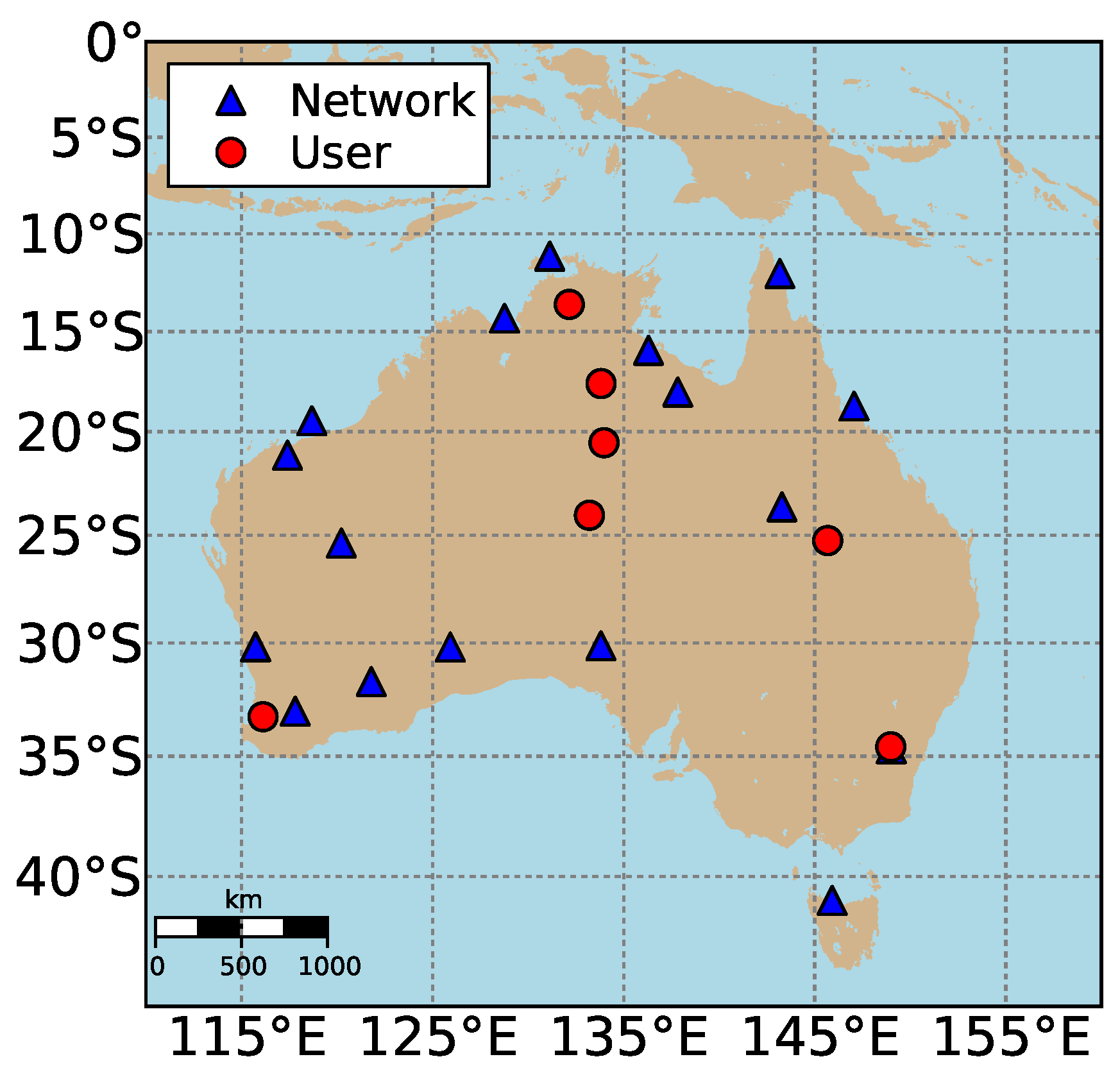
2.2. Experimental Setup

In this study, the processing is performed using 30-s Galileo code and phase observations on E1, E5a, E5b, E5 and E6, collected by continuously operating reference stations (CORS) belonging to the Australian Regional GNSS Network (ARGN) on three days starting from DOY 166 of 2020, which is an arbitrary choice. The geographic distribution of the 17 network stations for the estimation of network corrections and of the seven user stations for PPP-RTK positioning is shown in Figure 1. All stations are equipped with Septentrio PolaRx5 receivers, which are able to track all five frequency signals of Galileo. The cut-off elevation mask for all the data analysis in this work is set as 10${}^{\circ }$.

In our analysis, the precise Galileo satellite orbits calculated by the Centre for Orbit Determination in Europe (CODE), as part of the Multi-GNSS Experiment (MGEX) [35], were used as the known parameters for both network and user components. The ground-truth coordinates of the stations were retrieved from Geoscience Australia [36] and were used as known parameters in the network processing, while in the user processing they served as a means of evaluating the positioning errors. Concerning the receiver and satellite phase center offsets (PCOs) and variations (PCVs) for our network and user processing, we used the official antenna calibration file (igsR3_2107.atx: provided by Dr. Arturo Villiger (Astronomical Institute of the University of Bern)) used in the 3rd International GNSS Service (IGS, [37]) data reprocessing campaign. The selection of network and user stations was based on the availability of multi-frequency calibration information for the antennas that the stations are equipped with. In addition, a priori ZTD corrections are computed based on Saastamoinen’s model [38] with the Ifadis tropospheric mapping function [39]. The observation weights of the satellite s were calculated using the natural exponential function $\exp \left(·\right)$ based on the elevation angle ${\beta }_r^s$ (in degrees) [40]:

$$w_r^s={\left(1+10\exp \left(-\frac{{\beta }_r^s}{10}\right)\right)}^{-2}$$

(8)

In both network and user data processing, the estimable parameters listed in Table 1 are estimated in a Kalman filter, the initialization of which is performed with a standard least-squares estimation based on the data of the first epoch. The phase ambiguities, receiver/satellite phase and code biases are assumed to be time-constant, while the temporal behaviour of the ZTDs is modeled by a random-walk process with system noise of 0.1 mm$/\sqrt{30\mathrm{s}}$. The position components, receiver/satellite clocks and slant ionospheric delays are assumed to be completely unlinked in time. Therefore, our user processing is restricted to kinematic-only processing, while no prior spatial or temporal ionospheric information is used. The uncombined code and phase data were empirically assigned with a zenith-referenced standard deviation (STD) of 30 cm and 3 mm, respectively, which is a reasonable choice for most applications [41]. For the detection and identification of outliers, such as phase slips, we made use of the recursive Detection, Identification and Adaptation (DIA) procedure [42]. We remark here that the data in both network and user components are processed in emulated real-time mode, since only forward filter processing is performed.

After computing the ambiguity-float solutions in the Kalman filter, the user’s double-differenced ambiguities are decorrelated and fixed to their integers with the integer least-squares (ILS) estimator, which is efficiently mechanized in the Least-squares AMBiguity Decorrelation Adjustment (LAMBDA) method [43]. As a measure for successful ambiguity resolution, we use the formal integer bootstrapping (IB) success rate, which lower bounds the success rate of the optimal ILS estimator [44]:

$$P({\check{a}}_{\mathrm{ILS}}=a)=P({\check{z}}_{\mathrm{ILS}}=z)\ge P({\check{z}}_{\mathrm{IB}}=z)=\prod _{i=1}^{f(m-1)}\left(2\Phi \left(\frac{1}{2{\sigma }_{{\widehat{z}}_{i|I}}}\right)-1\right)$$

(9)

with $\Phi \left(x\right)$ denoting the cumulative normal distribution function:

$$\Phi \left(x\right)={\int }_{-\infty }^x\frac{1}{\sqrt{2\pi }}\exp \left(-\frac{u^2}{2}\right)du$$

(10)

where $P\left(·\right)$ denotes the formal ambiguity success rate; a and z denote the vectors of true but unknown original and transformed ambiguities, respectively, while the use of $\widehat{}$-symbol indicates the determined integers; ${\sigma }_{{\widehat{z}}_{i|I}}$ with $I=i+1,\dots ,f(m-1)$ stands for the conditional standard deviations of the decorrelated ambiguities, which are calculated as the square roots of the entries of the diagonal matrix D after an $L^{\mathrm{T}}DL$-decomposition of the decorrelated ambiguity vc-matrix. In our analysis, we consider the ILS-based partial ambiguity resolution (PAR) strategy that defines the to-be-resolved ambiguity subset based on a minimum success rate [45] that is defined as equal to 99.9%.

3. Experimental Results and Analysis

3.1. Formal Analysis

To obtain an understanding of the impact of the number and spacing of frequencies in standalone Galileo ambiguity resolution and an insight into the real data results presented in the next section, we formally analyze the user’s ambiguity resolution performance.

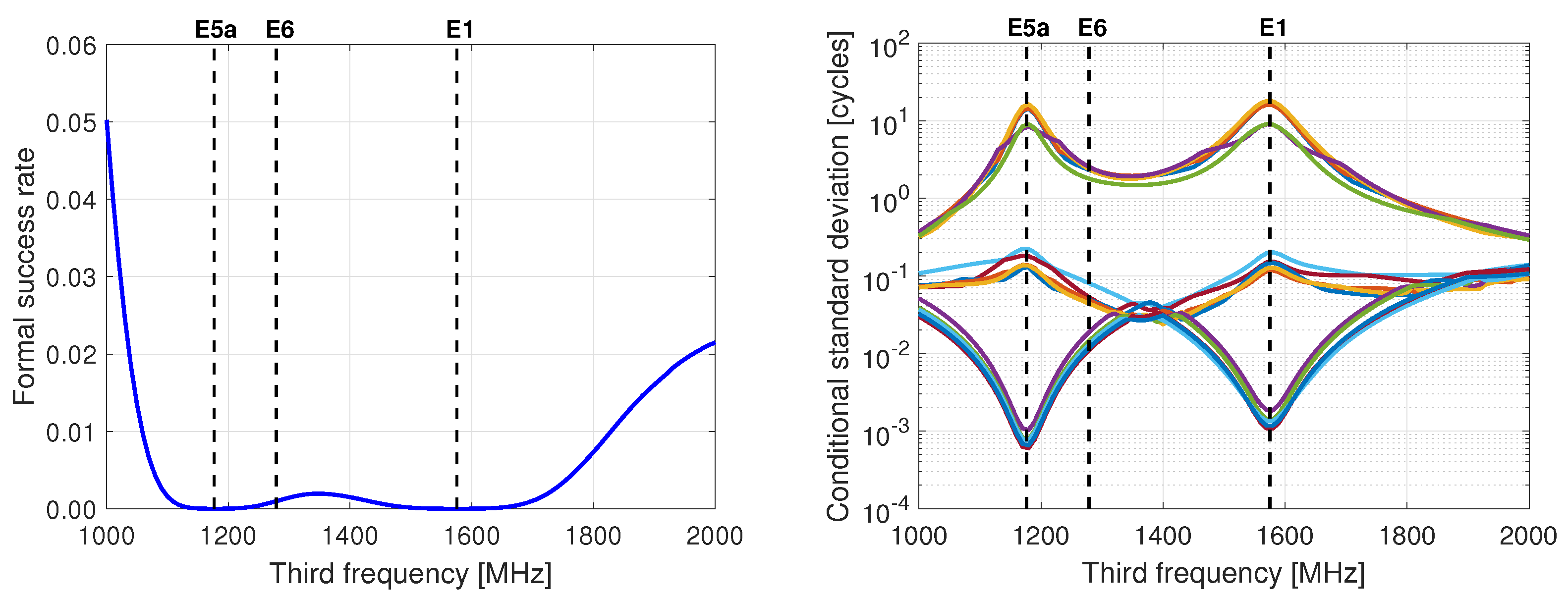
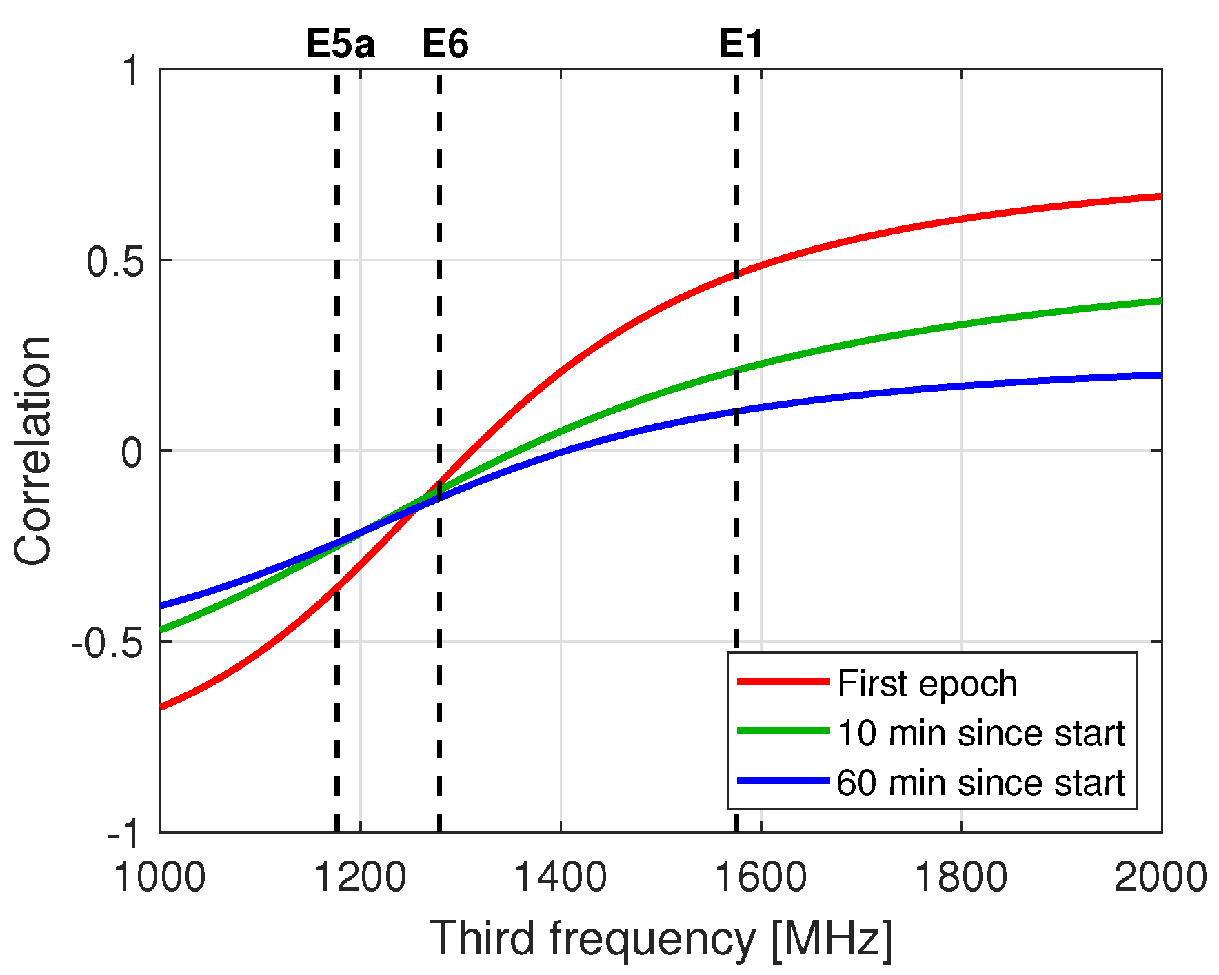
3.1.1. Frequency Spacing

Successful ambiguity resolution is key to the realization of PPP-RTK user positioning [4,46]. As a measure to analyze the full-ambiguity resolution (FAR) capabilities of the Galileo multi-frequency model, we use the formal success rate in Equation (9). The FAR success rate acts as an objective measure of the ambiguity resolution quality, and allows us to obtain a clear insight into the added value of the more-than-two frequencies and the importance of frequency separation in ambiguity resolution.

We remark here that in the multi-frequency analysis presented here and in the following, we use E1 and E5a as ‘starting’ frequencies. We reasonably consider this a natural choice for a multitude of reasons. First, the combination E1+E5a is the most commonly used dual-frequency combination in Galileo related studies, see, e.g., [8,10,12,19], while these frequencies allow for the interoperability of GPS and Galileo in mixed-system positioning due to the overlapping frequencies L1/E1 and L5/E5a [47]. Moreover, most of the MGEX analysis centres provide E1/E5a-based ionosphere-free clock products for the Galileo satellites [48]. Last but not least, E1 and E5a serve as the edge frequencies of Galileo, since they are the ones that are most apart in the frequency domain, which allows us to observe several patterns, formed by the addition of extra frequencies in terms of frequency separation.

We start our analysis by selecting a single epoch on DOY 166 of 2020, where six Galileo satellites are visible from station MTCV (denoted as a user station in Figure 1). Figure 2 (left) shows the single-epoch, ionosphere-float, triple-frequency formal ambiguity success rates as a function of a varying third frequency. The first two frequencies are held constant to E1 and E5a, and we assumed a frequency-independent zenith-referenced code and phase formal precision of 30 cm and 3 mm, respectively. We show the location of the E6 signal in the figure for convenience in our discussion, while the locations of E5b and E5 are not shown for clarity, as they are very close to E5a. When compared to the almost zero success rate of the dual-frequency model at the same epoch, the figure shows that the addition of a third frequency can improve the success rate. However, it is clear that it is at such low levels that successful ambiguity resolution at a single epoch is not possible, indicating the incapability of an ionosphere-float model to perform instantaneous ambiguity resolution with this setup.

To explain the signature of the success rate curve, we consider the conditional STDs of the LAMBDA-transformed ambiguities, which are provided by the square roots of the entries of the diagonal matrix D after an $L^{\mathrm{T}}DL$-decomposition of the decorrelated-ambiguity vc-matrix. We stress here that an analysis of the formal ambiguity STDs is far from sufficient to judge the ambiguity resolution performance. This would be possible only if the ambiguities were uncorrelated. Therefore, the precision of the transformed ambiguities, due to the decorrelation involved, can serve to explain the success rate curve to a good approximation. Figure 2 (right) shows the precision curves of the transformed ambiguities as a function of a varying third frequency. One can observe that some of the transformed ambiguities are of high precision, while others are of poor precision. As a result, the signature of the precision curves of the poorly determined ambiguities will dominate the typical shape of the success rate curve.

Further, Figure 2 shows that the success rate curve reaches its minimum values when the third frequency is selected to be at one of the two ‘starting’ frequencies, with these two minima being of the same order as the dual-frequency success rate. Although not distinguishable from the figure, we confirm that these two minima are not equal to zero, as would be the case for the rank-deficient dual-frequency model with two identical frequencies. The reason for this is that not all three frequencies are identical, which prevents us from a rank deficiency issue. The minima and maxima of the precision curves shown in the figure are explained as follows. When the third frequency is selected to be equal to the first one, i.e., $f_3=f_1$, one is able to estimate the difference between the first- and third-frequency ambiguities using only the phase data, therefore with very high precision. The case when $f_3=f_2$ is similar. This explains the two minima in the higher-precision curves at the bottom of the graph. In these cases, however, there are also ambiguities that cannot be determined in a phase-only solution and require the presence of code data. It is, therefore, the poor precision of the code data that leads to high standard deviations and, therefore, to the two maxima shown in the lower-precision curves.

In addition, it is evident that the success rate gets larger with larger frequency separation and that an improved ambiguity resolution performance is expected if the third selected frequency is as far as possible from E1 and E5a. Identical conclusions have been drawn for GPS long-baseline ambiguity resolution [49]. Given that the overall success rate is an objective measure of the quality of FAR, one can conclude that the selection of E6 as the third frequency in E6-capable receivers, and of E5b in E6-non-capable receivers, would be more beneficial than others in achieving higher success rates.

From the results of Figure 2, it is clear that an increase in the number of frequencies from two to three, even with large frequency separation, does not really ‘push’ the single-epoch success rates closer to the ideal value of one. Therefore, we consider an increasing number of epochs and assess whether the impact of number and spacing of frequencies is more pronounced. In our multi-epoch model, we consider the receiver phase biases, receiver code biases and phase ambiguities as time-constant parameters, while the other parameters are treated as being unlinked in time. The multi-epoch triple-frequency success rate curves as a function of a varying third frequency and a varying number of considered epochs are shown in Figure 3 (left). Note that these results are linked to the selected 30 s sampling rate, while the use of a higher data rate would improve the user performance. Although ambiguity resolution benefits from a low sampling rate due to the greater change in receiver-satellite geometry as times goes on, a higher sampling rate leads to a model of higher strength within the same timespan.

First, the results in Figure 3 (left) show that higher FAR success rates can be achieved by increasing the number of epochs and depict how the former is driven by the selection of the third frequency. The dual-frequency success rates are also shown in the figure with horizontal dashed lines. Compared to the dual-frequency performance, one can observe that, with an additional frequency, one ends up with higher FAR success rates, with the improvement being more prominent with an increased number of epochs. Regarding frequency separation, one clearly observes its distinct effect in the multi-epoch setup, with the addition of a third frequency far away from E1 and E5a being able to considerably increase the user success rate. As an example, the success rate would be equal to about 50% by selecting E5b as the third frequency after 20 epochs, while this would increase to 80% by selecting E6. After 30 epochs, the success rates would be 82% and 95%, respectively. Thus, we observe that the impact of increased number of frequencies is heavily pronounced in the first epochs, while it is rather modest after a considerable amount of accumulated epochs, since the model is already strong.

The above results underline the importance of an increased number of frequencies, which can boost the user ambiguity resolution capabilities. In achieving the highest possible FAR success rates, the user should opt for signals with frequencies that are as far as possible from the two ‘starting’ ones. Since a considerable amount of time is needed to achieve reliable FAR with a success rate higher than $99.9\%$, we opt to fix only a subset of the ambiguities with the same criterion in order to obtain a considerable precision gain in shorter time. In the top-right panel of Figure 3, we present the positioning precision gain after successful PAR as the ratio of the float and fixed horizontal positioning precision, as a function of a varying third frequency and an increasing number of epochs. We reasonably opt to show the precision gain after PAR, rather than the formal success rate, as done in FAR, because the PAR success rate, by definition, is larger than $99.9\%$, and therefore not sufficient to show the contribution to the user performance.

The results in the top-right panel of Figure 3 confirm that frequency separation plays a dominant role also in PAR-based user performance, as the further the third frequency is from the ‘starting’ frequencies, the larger the gain. With an increased number of epochs involved, we see an increase in the position precision gain as well, due to the fact that more ambiguities become precise enough to be included in the fixable PAR-subset. We make clear, however, that no direct comparison of the precision-gain curves can be made, since the gains depend on the ambiguity-float horizontal position precision that also improves with more epochs. This becomes clear if one observes the 30- and 60-epoch precision gain curves that are shown with the blue and purple color, respectively. Although one would intuitively think that a larger gain should be expected when 60 epochs are used, the achievable gain with 60 epochs is smaller than the one with 30 epochs because of the higher precision of the 60-epoch-based ambiguity-float position solution. We recall here that, over a sufficiently large time interval, the ambiguity-float solution will share the same quality as the ambiguity-fixed counterpart, leading to a gain value of 1, because the former becomes more precise over time.

Note that a precision gain value of 1 indicates that either ambiguity resolution cannot be reliably executed, leaving the user only with a float solution, or that the ambiguity-resolved performance is equivalent to the ambiguity-float counterpart. The bottom-right panel of Figure 3 shows the availability of successful FAR and PAR for a varying third frequency, that is, when the success rate criterion of $99.9\%$ is exceeded. It is very interesting to note that PAR is shown to be feasible in an instant for frequencies between E1 and E5a, including those of E5b, E5 and E6. However, the corresponding precision gains are shown to be equal to approximately 1. To understand the underlying reasons for this behaviour, we conducted an inspection of the conditional standard deviations of the transformed ambiguities and the LAMBDA Z-transformation matrix. For all the frequencies between E1 and E5a, we found out that the fixable ambiguities are wide-lane-like ones, while when the third frequency is closer to E1 or E5a (e.g., E5 and E5b), only the extra-wide-lane ambiguities are fixable. It is shown, therefore, that fixing these widelanes hardly improves the partially-fixed positioning precision, thereby the value of 1.

It is worth mentioning here that although we focused on Galileo and its existing frequencies in our formal analysis, the concept and results discussed above are generally applicable to any GNSS system and can easily serve to show the achievable gain after ambiguity resolution when more than two frequencies are employed, e.g., with BeiDou-3 multi-frequency data.

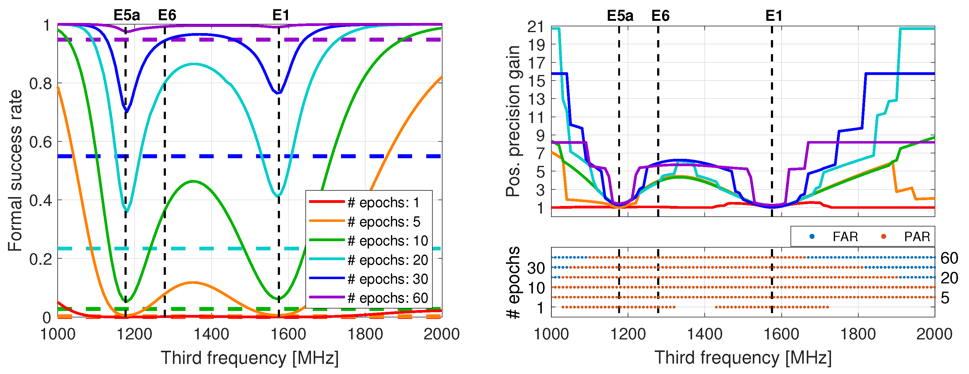
3.1.2. More Frequencies, Shorter Convergence Time?

The question that comes now naturally to the fore is how much time is representatively needed to achieve reliable partially-fixed solutions based on the number and spacing of frequencies. To do so, we compute multiple hourly Galileo-only Kalman-filtered kinematic user positioning solutions with PAR in a formal analysis setup. Based on the conclusions of the previous section, it would make sense to consider E6 as the third frequency when operating with an E6-capable receiver, while E5b should be considered with other receivers. For compactness in our study, and due to the fact that only a minority of receivers currently support E6, we naturally consider E5b as the third frequency, E5 as the fourth, and E6 as the fifth. In such a setup, we are able to present results that are representative of an E6-non-capable receiver, as well as results for the current and future E6-capable ones with the further addition of E6. As the combination E1+E5a+E6 was shown to be the natural triple-frequency choice in an E6-capable receiver in the ambiguity resolution sense, we decide to also show results for this combination for completeness.

The timespans needed for the formal horizontal positioning precision values (90% percentiles) to be better than 10 cm are listed in

Table 2. Time span (in minutes) needed for the standalone Galileo, multi-frequency, ionosphere-float, PAR-based, kinematic PPP-RTK user models to obtain formal positioning precision better than 10 cm in 90% of the cases, with and without the provision of satellite code bias corrections.

	Provision of Satellite Code Biases	Estimating Satellite Code Biases
E1+E5a+E5b	17.5	18.0
E1+E5a+E5b+E5	16.0	18.0
E1+E5a+E6	13.0	13.0
E1+E5a+E5b+E5+E6	12.0	12.5

The corresponding time span for the standalone Galileo dual-frequency solution is 31.0 min. Satellite code biases are treated, when estimated, as time-constant parameters.

. One can observe that the convergence time of the formal solutions is improved with an increased number of frequencies. It is further seen that the dual-frequency user enjoys a considerable improvement by adding E5b, but a much smaller increase after adding E5 as the fourth frequency, due to the small frequency spacing between E5 and the involved signals.

With the further integration of E6, which was previously shown to significantly boost the user ambiguity resolution capabilities due to its large spacing with the other frequencies, one easily notes a substantial decrease in the time needed to reach the 10 cm level. It is important to mention here that the E1+E5a+E6 triple-frequency integration outperforms the E1+E5a+E5b+E5 combination in the sense of fast successful ambiguity resolution, due to the fact that E6, compared to E5b and E5, has a larger frequency spacing from E1 and E5a. This underlines the pivotal role of frequency separation, since the user can achieve better performance with fewer frequencies, given that they are widely spaced. Therefore, when evaluating the user ambiguity-resolved performance, one should not only consider the number of frequencies involved but, even more importantly, the spacing between the already used and additional frequencies. In cases where all available Galileo signals are integrated, we observe that the convergence time is the shortest among all cases.

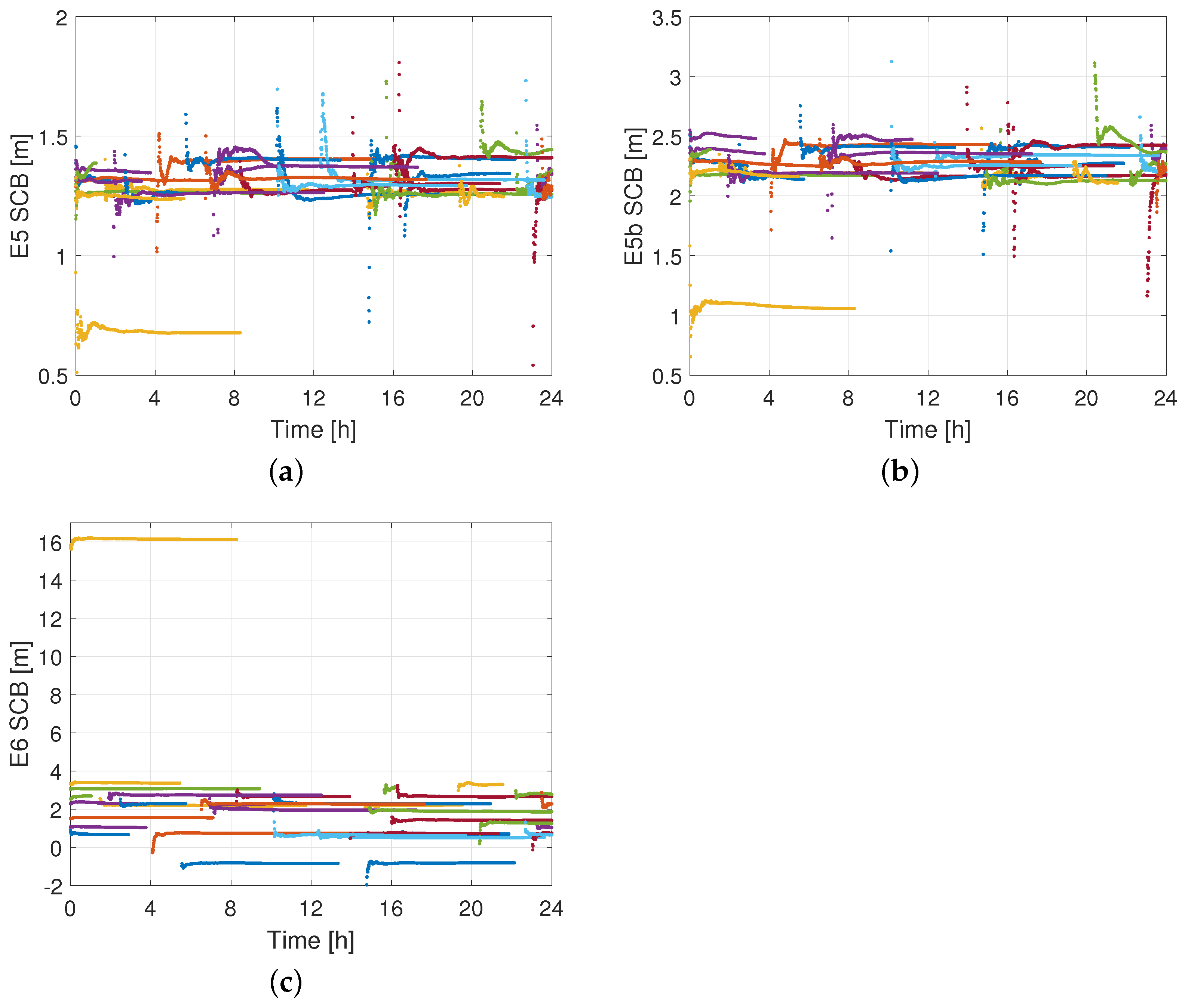
3.1.3. Impact of Satellite Code Bias Corrections

It is also of interest to gain insight into the role of the satellite code bias corrections in speeding up user convergence through the increased model redundancy. To do so, we compute the formal positioning solutions with the same settings as used previously, with the only difference being that the satellite code biases are estimated as time-constant parameters, instead of being corrected for. The results in Table 2 reveal that the provision of the satellite code biases brings a reduction of up to 2.0 min in the formal user-convergence (90% percentile). When the code precision improves, their contribution is expected to be larger, especially during the initial convergence that relies on the code data (cf. Section 3.1.1). It is interesting to see that the E1+E5a+E6 model requires the same timespan to reach 10 cm in both the presence and absence of satellite code biases, which is due to the frequency-dependent correlation of the latter with the user-ambiguities.

Figure 4 presents the correlation coefficient between the user-estimated satellite code biases and float ambiguities of a representative individual satellite as a function of a varying third frequency. The stated correlation is shown to range up to 0.65 (in magnitude). Moreover, it is observed that the correlation for E6 is smaller than that for E5b and E5. Therefore, one expects that the provision of the satellite code bias corrections will have a stronger impact on user ambiguity resolution and convergence performance when E5 or E5b is selected as the third frequency than when E6 is used.

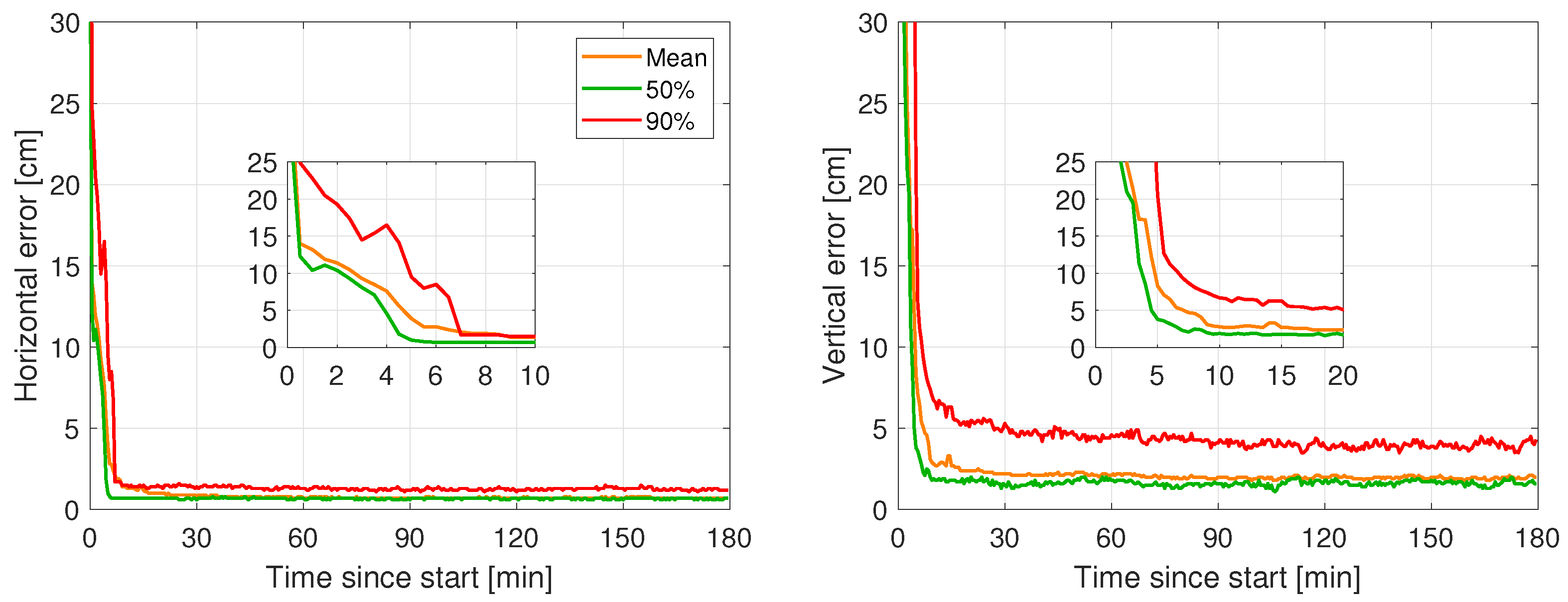
3.2. Empirical Analysis

In this section, we use real data to verify the formal analysis findings and assess the empirical user convergence times of multi-frequency Galileo-only and Galileo+GPS PPP-RTK positioning.

3.2.1. Network Corrections

We first estimate with a Kalman filter the network corrections needed to realize single-receiver, multi-frequency PPP-RTK positioning in real-time. These corrections consist of the satellite clocks, satellite phase (SPBs) and code biases (SCBs). We chose to determine the estimable code biases, rather than obtaining DCBs from an external source as in Li et al. [50], in order to have a consistent estimation of the highly correlated PPP-RTK corrections. Based on our observation model and chosen $\mathcal{S}$-basis (cf. Section 2.1), as well as a rigorous integration of the network’s redundant data, we estimated SPBs on all five frequency signals and SCBs on the higher-than-two frequencies, which are E5b, E5 and E6 in our case. That is, we selected E1 and E5a as the ‘starting’ frequencies so that our estimable satellite clocks were similar to those of most MGEX analysis centres. The estimable SCBs are observable-specific signal biases and can be directly applied to the uncombined code data from the third frequency onwards to strengthen the user’s model. For brevity, we hereafter present only the SCB estimates.

Figure 5 presents the multi-frequency code bias estimates of the Galileo satellites on DOY 166 of 2020. It can be seen that the code biases of all satellites show, after their initial convergence period, remarkable time-stability. Moreover, one can observe another interesting feature of the E5b and E5 SCBs. For most of the Galileo satellites the E5b and E5 code biases fluctuate within a narrow range of about 50 and 25 cm, respectively. Given that these estimable satellite code biases are functions of the modern and legacy DCBs (cf. Equation (3)), and due to the magnitude of the coefficient $({\mu }_j-{\mu }_1)/({\mu }_2-{\mu }_1)$ of one of them that is close to the value one for these frequencies, one may reasonably conclude that the absolute satellite code biases on E5a, E5b and E5 are almost identical. As a result, the satellite DCBs between E5b and E5 signals are almost zero, as also shown in Li et al. [50]. The only exception to this case is satellite E24, for which a code bias of larger magnitude is seen, while high differential biases have also been reported earlier in Ammar et al. [51]. In the case of E6, we observe that the satellite code biases do not fluctuate within a narrow range, unlike E5b and E5, indicating that the satellite DCBs between E6 and the other signals are not equal to zero. For the same reason as before, the E6 code bias of satellite E24 shows a large offset compared to those of the other satellites.

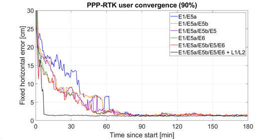
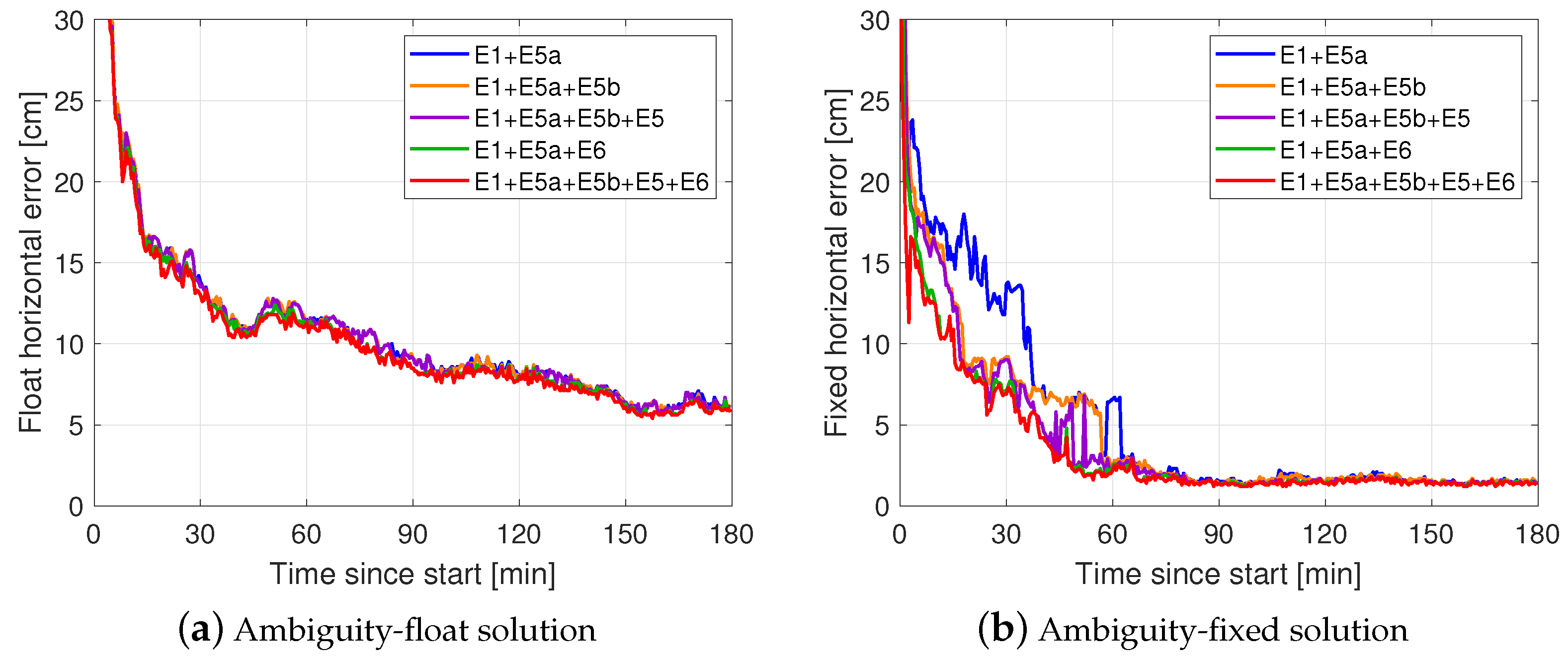
3.2.2. Galileo-Only PPP-RTK Positioning

With the network-derived multi-frequency satellite corrections applied in the code and phase data (cf. (5)), the user positioning performance, in terms of the achieved convergence times, is analyzed using real data from the seven user stations shown in Figure 1. The user-processing strategy was discussed in Section 2.2. To infer the empirical distribution of the achieved convergence times and realistically judge the standalone Galileo multi-frequency performance, we aimed to obtain a representative sample of solutions. We did this by processing the Galileo data of all user stations with a 3-h processing window being re-initialized every minute over the selected three days so as to capture all possible receiver-satellite geometries. The user’s positioning errors were computed using precise benchmark coordinates and sorted for each epoch according to their absolute magnitude. From this set, we then identified the mean, 50% and 90% percentile values of the horizontal and vertical errors, resulting into convergence curves that are used in the following to characterize the user’s achieved performance. We remark here that convergence time, in this study, is defined as the time interval needed for the horizontal and vertical positioning errors to go below and stay below 10 cm (or 5 cm). Note also that the ‘starting’ frequencies used are E1 and E5a, while the multi-frequency models are based on integrating first E5b and then E5 to obtain results for E6-non-capable receivers, and later E6 to cover the E6-capable receivers. For the sake of completeness, we also show results for the E1+E5a+E6 solution, as in Section 3.1.

Figure 6 shows the convergence behaviour of the standalone Galileo multi-frequency ambiguity float (left panel) and PAR-fixed (right panel) kinematic horizontal radial positioning errors, whereas those for the vertical errors are not shown for brevity, but their achieved convergence times in both ambiguity float and fixed setups are listed in

Table 3. Convergence time (in minutes) of standalone Galileo, multi-frequency, ionosphere-float, kinematic PPP-RTK user positioning solutions to achieve horizontal and vertical accuracy better than 10 cm (and 5 cm in square brackets). The mean, 50% and 90% percentiles are provided.

	Horizontal			Vertical
	Mean	50%	90%	Mean	50%	90%
Float
E1+E5a	13.0 [67.0]	9.5 [34.5]	84.5 [ - ]	45.5 [132.0]	26.0 [74.5]	130.0 [ - ]
E1+E5a+E5b	13.0 [67.0]	9.5 [34.5]	84.5 [ - ]	45.5 [132.0]	26.0 [74.5]	127.5 [ - ]
E1+E5a+E5b+E5	12.5 [67.0]	8.5 [34.5]	84.5 [ - ]	45.0 [132.0]	25.5 [74.0]	127.5 [ - ]
E1+E5a+E6	12.5 [67.0]	8.5 [30.0]	75.0 [ - ]	45.0 [132.0]	25.5 [69.0]	127.5 [ - ]
E1+E5a+E5b+E5+E6	12.5 [67.0]	8.5 [30.0]	75.0 [ - ]	43.5 [105.0]	24.5 [69.0]	127.5 [ - ]
Fixed
E1+E5a	12.5 [33.0]	8.0 [24.5]	37.0 [62.5]	35.0 [ 62.5]	22.0 [28.0]	64.0 [144.0]
E1+E5a+E5b	5.5 [18.0]	3.5 [15.5]	18.0 [57.0]	27.0 [ 52.5]	14.0 [22.5]	53.0 [144.0]
E1+E5a+E5b+E5	5.0 [17.5]	3.5 [14.0]	17.0 [52.5]	24.5 [ 48.5]	14.0 [21.5]	49.0 [120.5]
E1+E5a+E6	4.5 [15.5]	3.5 [10.0]	15.0 [39.0]	23.5 [ 38.5]	13.5 [19.5]	38.0 [ 83.0]
E1+E5a+E5b+E5+E6	3.5 [15.0]	2.0 [ 9.5]	15.0 [39.0]	20.5 [ 38.5]	13.0 [18.0]	38.0 [ 83.0]

The convergence time is defined as the timespan needed for the positioning errors to go below and stay below 10 cm (or 5 cm). The convergence times indicated with a dash denote that no convergence was achieved within the 3-h time windows. Note also that the mean, 50% and 90% percentiles were calculated on the basis of all user stations in 3-h time windows being re-initialized every 1 min within the selected days. The PAR success rate criterion was set to 99.9%.

. The ambiguity-float solutions, with time-constant ambiguities, gain a high accuracy over time, because the float ambiguities become more precise over time and, as a result, the positioning accuracy is dictated by the very precise phase data. Adding more frequencies to the system seems to bring only slight improvements, with similar results being shown in Guo et al. [29], due to the invariance of satellite geometry [52]. It is clear that the float solutions do not converge to 5 cm within the first 3 h, and the results in Table 3 reveal that more than 1 h is needed for the horizontal errors to go below and stay below 10 cm for all multi-frequency solutions.

Moving from the float solutions in the left panel to the fixed solutions in the right panel of Figure 6, a performance gain via ambiguity resolution is evident. In particular, considering the model-driven PAR strategy for resolving the integer ambiguities, we observe a rapid decrease in the horizontal positioning errors, with the dual-frequency solution going below and staying below 10 cm after 37 min, which is an about 56% improvement compared to the float solution. When the model is of sufficient strength and all ambiguities are successfully fixed, a positioning accuracy of 1.5 cm is achieved on a continuous basis.

The integration of E5b as the third frequency seems to considerably improve the user’s performance, as is also demonstrated in our formal analysis, with the reduction in convergence time being about 50% compared to the dual-frequency fixed solution, while the further addition of E5 leads only to a marginal improvement. This is due to the fact that, in the absence of E6, it is E5b that offers larger frequency separation than E5 in the triple-frequency setup. The additional inclusion of E5 does not boost the performance, as its frequency is between and very close to the ones of E5a and E5b.

The transition to the penta-frequency solution considers the use of the E6 signal. We observe in Figure 6 that the PPP-RTK user benefits from the integration of all Galileo frequencies, as predicted by the formal analysis, since the time needed for the horizontal errors to go below and stay below 10 cm is 15 min, the shortest one among all multi-frequency models and 12% shorter than the four-frequency one. The main reason for this performance lies in the improved model strength with regard to ambiguity resolution, as a result of the frequency separation that E6 offers (cf. Section 3.1.1). An even greater improvement is seen for the convergence time to 5 cm, of about 26%, with the integration of E6. Shortened convergence times are also observed for the vertical component. Compared to the dual-frequency fixed vertical solution, the inclusion of the third, fourth and fifth frequency brings a convergence time reduction of 17%, 23% and 41%, respectively.

Figure 6 and Table 3 also show the achieved convergence time of the E1+E5a+E6 solution. Our formal analysis revealed that this is the triple-frequency combination that brings the largest benefit in terms of ambiguity resolution in E6-capable receivers, as shown here. Interestingly enough, we observe that the convergence curves of the E1+E5a+E6 and penta-frequency solutions almost overlap, with their 90% percentiles being equal, as was well predicted in our formal analysis (cf. Table 2). The penta-frequency solution seems to perform only slightly better when assessing the mean and 50% values. Thus, from a convergence point of view, the addition of E5b and E5 does not boost the E1+E5a+E6 solution, because of the vicinity of E5b and E5 to E5a and because the largest possible frequency spacing was already harnessed after integrating E6 with E1+E5a. This result confirms our formal analysis finding that the user ambiguity resolution capabilities are mainly driven by the frequency spacing and, to a smaller extent, by the number of additional frequencies.

As in our formal analysis, we consider it essential to provide numerical insight into the empirical user-convergence in the absence of satellite code bias corrections. As such, we process the multi-frequency Galileo data of all user stations with the same settings as used previously, but treating the satellite code biases as time-constant parameters.

Table 4. Convergence time (in minutes) of standalone Galileo, multi-frequency, ionosphere-float, kinematic PPP-RTK user fixed horizontal positioning solutions (90% percentiles) with and without the provision of satellite code bias corrections.

	Provision of Satellite Code Biases	Estimating Satellite Code Biases
E1+E5a+E5b	18.0	22.0
E1+E5a+E5b+E5	17.0	21.0
E1+E5a+E6	15.0	16.0
E1+E5a+E5b+E5+E6	15.0	15.5

The convergence time is defined as the timespan needed for the positioning errors to go below and stay below 10 cm.

lists the empirical convergence times (90% percentiles) of the multi-frequency models to achieve a horizontal error that is consistently below 10 cm. From the numerical results shown, one can observe that the multi-frequency PPP-RTK user-convergence benefits by applying externally provided satellite code bias corrections, as was well predicted by our simulations. Unlike the formal analysis results, we observe here that the E1+E5a+E6 solution benefits from external satellite code biases, despite the small correlation of user-estimated ambiguities and satellite code biases for E6. The small differences from the formal results (cf. Table 2) are due to the fact that the latter makes use of only the design and vc-matrices, not real data. We remark here that one can still perform ambiguity-resolved positioning in the absence of such corrections, but with a penalty in the achieved convergence times in the order of a few minutes. Note also that the stronger the user model is in terms of its ambiguity resolution capabilities, the less the convergence sensitivity becomes. From the results shown, one can conclude that the provision of the satellite code biases as standard corrections to multi-frequency PPP-RTK users is essential to fully exploit the user code data from the third and following frequencies, thereby accelerating convergence.

3.2.3. Galileo+GPS PPP-RTK Positioning

Standalone Galileo was shown to be weak to support fast centimeter-level positioning with reliable integer ambiguity resolution in the presence of ionospheric delays. Our real data analysis demonstrated that its five-frequency signal integration is able to significantly speed up the user’s convergence, with 90% of the computed horizontal positioning solutions requiring 15 min to reach an accuracy equal to or better than 10 cm. In this section, we investigate the feasibility of achieving rapid convergence with the integration of GPS data in an ionosphere-float setup, i.e., without any prior spatial or temporal information about the ionosphere. We focus here on the use of GPS dual-frequency data, since L5 is transmitted only by GPS Block IIF satellites.

The GPS network-derived positioning corrections were computed based on the same network that was used for the generation of the Galileo corrections, on the basis of the processing strategy in Section 2.2. In the next step, the GPS and Galileo network-derived positioning corrections were applied to correct the code and phase data of all user stations, and positioning solutions were obtained in 3-h time windows that were shifted and re-initialized every minute to obtain a representative sample of solutions. In this process, the user settings were identical to those of the standalone Galileo processing. Note also that, in the combined system analysis, the systems were treated separately, with only the receiver position increments and ZTD being common for the systems. That is, one reference satellite was taken per system, and not a common one across systems to exploit the overlapping frequencies. Given the computed solutions and the precise benchmark coordinates, the horizontal radial and vertical positioning errors were computed per epoch, from which the convergence curves are determined.

In the following, the positioning results of the combined model are visualized and further discussed. Figure 7 shows the mean, 50% and 90% percentiles of the partially-ambiguity-fixed positioning errors as a function of time for Galileo+GPS kinematic positioning. The benefit of integrating multi-GNSS multi-frequency data is evident. With the combined system, one can observe that fast and reliable ambiguity resolution can be achieved much faster than when using only Galileo data (cf. Figure 6), which is obvious from the significantly steeper convergence curves.

Making use of the provided zoom-in windows, we can observe that the mean and 90% percentiles of the ambiguity-fixed horizontal positioning errors become smaller than 10 cm after 3.0 and 5.0 min, respectively. This result shows the advantage of integrating GPS with Galileo data, as the average number of satellites increased from almost 7 in the Galileo-only setup to 16 in the combined-system setup. Therefore, we provide supporting evidence that rapid centimeter-level PPP-RTK positioning can actually be obtained with this combined model in the absence of any prior information for the ionosphere. This is of great importance for single-receiver users, as they can quite rapidly reach centimeter-level accuracy, even when they do not operate within a dense network of receivers, so that they benefit from regional ionospheric corrections (cf. [5,6,53]).

Such a gain in performance is also observed in the vertical positioning results. We observe that the vertical positioning errors are better than 10 cm after 7.0 min in 90% of cases, or after 5.0 min on average. The achieved vertical positioning accuracy, after convergence, is 4.3 cm. With these results in mind, we show that applications requiring fast high-accuracy results also in the vertical component can benefit from the combined system.

4. Discussion

With the rapid development of navigation satellite systems, there is an increase in the number of available GNSS frequencies. The integration of data over multiple frequencies increases the user model’s redundancy, thus providing a stronger positioning model, and therefore raising the potential for faster PPP-RTK ambiguity resolution.

In this contribution, we focus on the multi-frequency capabilities provided by the European Galileo system and present a thorough analysis of the role of additional frequencies in improving the user ambiguity resolution and positioning performance. Although previous studies have shown that such an integration can lead to improvements, a proper understanding of the selection of frequencies that lead to optimal performance is missing. Using a formal analysis, we show that frequency separation has a more prominent role than the number of used frequencies in driving the ambiguity resolution performance, as shown in the comparison of the E1+E5a+E6 solution with the usually employed E1+E5a+E5b solution and with its five-frequency counterpart. Supported by real-data results, it was shown that the multi-frequency Galileo PPP-RTK solutions can achieve a 15 min convergence time at 90%.

Special emphasis is also placed on the role of the estimable satellite code biases from the third frequency onwards as standard PPP-RTK corrections. It has been a common practice in the literature to either ignore or estimate these biases at the user side. Through both formal and empirical analyses, we show that, in the presence of such corrections, an up to 4 min improvement in the convergence time can be expected, with the convergence sensitivity being reduced, the stronger the user model is in terms of its ambiguity resolution capabilities.

This analysis serves in providing a proper understanding of the role and intricacies of multiple frequencies in accelerating PPP-RTK user convergence. This is considered to be essential in light of the proliferation of navigation satellite systems, as one can choose to process only those signals that lead to optimal performance and avoid the potential computational slowdown that comes along with the increased ambiguity dimension.

5. Conclusions

In this contribution, we studied and presented the key role of multiple frequencies in PPP-RTK ambiguity resolution and numerically demonstrated the multi-frequency, ionosphere-float, standalone Galileo kinematic PPP-RTK positioning performance for an increasing number of frequencies up to five. As more frequencies provide a stronger model and, therefore, improved integer ambiguity resolution, we analyzed the role of the increasing number of frequencies, as well as their spacing, in speeding up the convergence times of kinematic users.

We started off with a detailed review of the PPP-RTK network and user observation models using uncombined, and therefore undifferenced, GNSS measurements. It was shown that, in the given $\mathcal{S}$-basis choice, the receiver and satellite code biases become estimable for the third and following frequencies without the explicit use of a prior ionospheric model, as is the usual practice. We emphasized that the provision of the satellite code biases as standard PPP-RTK corrections, through the increased user’s model redundancy, allows the multi-frequency user code data to properly contibute to the user solutions.

We then formally studied the user ambiguity resolution capabilities of the standalone Galileo multi-frequency model as a function of the number and spacing of frequencies. Using the full-ambiguity success rate as a tool to evaluate the ambiguity resolution performance, we showed that a single-epoch, ionosphere-float, triple-frequency PPP-RTK user model is too weak to support instantaneous ambiguity resolution. Although not very obvious in the single-epoch case, we demonstrated in the multi-epoch setup that frequency separation plays a dominant role in ambiguity resolution, as the further the third frequency is from the ‘starting’ two frequencies, the higher the success rate. Similarly, frequency separation was shown to have strong impact on the PAR-based positioning precision gain. It was, therefore, concluded that E5b would serve as the optimal third frequency choice in E6-non-capable receivers, while E6 would serve in E6-capable ones. Further, we computed multiple Kalman-filtered user solutions throughout a day to evaluate the formal user-convergence. It was found that increasing the number of frequencies can indeed accelerate convergence. More interestingly, we showed that frequency separation has a larger weight than the number of frequencies used in ambiguity resolution performance, which was evidenced by the fact that the E1+E5a+E6 solutions performed better than the E1+E5a+E5b+E5 counterparts, while the former had an almost identical performance with the E1+E5a+E5b+E5+E6 solutions.

In addition, the empirical ionosphere-float PPP-RTK user performance was assessed with real Galileo data from Australian stations on all five frequencies. In the prior step, that being the corrections’ generation, we found that the satellite code biases have a remarkable time-stability, and we showed that the absolute code biases of E5a, E5b and E5 are almost identical. Given the satellite PPP-RTK corrections, we computed a representative sample of standalone Galileo positioning solutions for an increasing number of frequencies up to five to realistically judge the user’s performance in terms of the achieved convergence times. We showed that the long convergence time of the dual-frequency ambiguity-float horizontal positioning errors to go below and stay below 10 cm was reduced from >1 h to 37.0 min (90% percentile) with PAR. The addition of E5b significantly reduced the convergence time to 18.0 min (90% percentile), while the further integration of E5 only marginally improved the performance due to the small frequency spacing. The penta-frequency solution, with the addition of E6 to the system, was shown to have, as a result of the large frequency separation, the shortest convergence time of 15.0 min in the horizontal component among all multi-frequency solutions. As was well predicted by our formal analysis, the E1+E5a+E6 solution had almost the same performance, indicating that it suffices to use these three signals to achieve the optimal Galileo-based performance. Then, we showed how and to what extent the satellite code bias corrections, provided as standard PPP-RTK corrections, contribute to the user-convergence. Through our numerical analysis, we demonstrated that, by correcting for the estimable code biases, the multi-frequency user code data properly contribute to speeding up the convergence time, with the improvement ranging up to 4.0 min.

Finally, we investigated the capabilities of the combined Galileo+GPS multi-frequency model to achieve rapid centimeter-level positioning. Using Galileo and GPS data and corrections from the same network in Australia, we numerically demonstrated that the kinematic PPP-RTK horizontal positioning errors required 3.0 min on average, and 5.0 min at 90% of cases, to go below and stay below 10 cm in the presence of ionospheric delays. This fast convergence to the centimeter level is of great importance, as it implies that a single-receiver user can achieve such rapid positioning results without the use of a precise ionosphere model and, more importantly, without the need for a dense reference network to provide regional atmospheric corrections. With the above real data results, we believe that more studies can be considered for achieving near-instantaneous PPP-RTK positioning by incorporating GLONASS, BeiDou and QZSS data, similar to the five-system analysis of Brack et al. [14].

References

1. Leandro, R.; Landau, H.; Nitschke, M.; Glocker, M.; Seeger, S.; Chen, X.; Deking, A.; BenTahar, M.; Zhang, F.; Ferguson, K.; et al. RTX positioning: The next generation of cm-accurate real-time GNSS positioning. In Proceedings of the 24th International Technical Meeting of the Satellite Division of the Institute of Navigation (ION GNSS 2011), Portland, OR, USA, 20–23 September 2011; pp. 1460–1475. [Google Scholar]
2. Banville, S.; Collins, P.; Zhang, W.; Langley, R. Global and regional ionospheric corrections for faster PPP convergence. Navigation 2014, 61, 115–124. [Google Scholar] [CrossRef]
3. Odijk, D.; Zhang, B.; Khodabandeh, A.; Odolinski, R.; Teunissen, P.J.G. On the estimability of parameters in undifferenced, uncombined GNSS network and PPP-RTK user models by means of S-system theory. J. Geod. 2016, 90, 15–44. [Google Scholar] [CrossRef]
4. Teunissen, P.J.G.; Odijk, D.; Zhang, B. PPP-RTK: Results of CORS network-based PPP with integer ambiguity resolution. J. Aeronaut. Astronaut. Aviat. 2010, 42, 223–230. [Google Scholar]
5. Li, X.; Zhang, X.; Guo, G. Predicting atmospheric delays for rapid ambiguity resolution in precise point positioning. Adv. Space Res. 2014, 54, 840–850. [Google Scholar] [CrossRef]
6. Psychas, D.; Verhagen, S. Real-Time PPP-RTK Performance Analysis Using Ionospheric Corrections from Multi-Scale Network Configurations. Sensors 2020, 20, 3012. [Google Scholar] [CrossRef] [PubMed]
7. Geng, J.; Li, X.; Zhao, Q.; Li, G. Inter-system PPP ambiguity resolution between GPS and BeiDou for rapid initialization. J. Geod. 2019, 93. [Google Scholar] [CrossRef]
8. Katsigianni, G.; Loyer, S.; Perosanz, F. PPP and PPP-AR Kinematic Post-Processed Performance of GPS-Only, Galileo-Only and Multi-GNSS. Remote Sens. 2019, 11, 2477. [Google Scholar] [CrossRef] [Green Version]
9. Liu, T.; Jiang, W.; Laurichesse, D.; Chen, H.; Liu, X.; Wang, J. Assessing GPS/Galileo real-time precise point positioning with ambiguity resolution based on phase biases from CNES. Adv. Space Res. 2020, 66, 810–825. [Google Scholar] [CrossRef]
10. Nadarajah, N.; Khodabandeh, A.; Wang, K.; Choudhury, M.; Teunissen, P.J.G. Multi-GNSS PPP-RTK: From Large- to Small-Scale Networks. Sensors 2018, 18, 1078. [Google Scholar] [CrossRef] [PubMed] [Green Version]
11. Li, P.; Jiang, X.; Zhang, X.; Ge, M.; Schuh, H. GPS+Galileo+BeiDou precise point positioning with triple-frequency ambiguity resolution. GPS Solut. 2020, 24, 78. [Google Scholar] [CrossRef]
12. Li, X.; Li, X.; Yuan, Y.; Zhang, K.; Zhang, X.; Wickert, J. Multi-GNSS phase delay estimation and PPP ambiguity resolution: GPS, BDS, GLONASS, Galileo. J. Geod. 2018, 92, 579–608. [Google Scholar] [CrossRef]
13. Ma, H.; Zhao, Q.; Verhagen, S.; Psychas, D.; Liu, X. Assessing the Performance of Multi-GNSS PPP-RTK in the Local Area. Remote Sens. 2020, 12, 3343. [Google Scholar] [CrossRef]
14. Brack, A.; Männel, B.; Schuh, H. GLONASS FDMA data for RTK positioning: A five-system analysis. GPS Solut. 2021, 25, 9. [Google Scholar] [CrossRef]
15. Geng, J.; Bock, Y. Triple-frequency GPS precise point positioning with rapid ambiguity resolution. J. Geod. 2013, 87, 449–460. [Google Scholar] [CrossRef]
16. Xiao, G.; Li, P.; Gao, Y.; Heck, B. A Unified Model for Multi-Frequency PPP Ambiguity Resolution and Test Results with Galileo and BeiDou Triple-Frequency Observations. Remote Sens. 2019, 11, 116. [Google Scholar] [CrossRef] [Green Version]
17. Liu, G.; Zhang, X.; Li, P. Improving the Performance of Galileo Uncombined Precise Point Positioning Ambiguity Resolution Using Triple-Frequency Observations. Remote Sens. 2019, 11, 341. [Google Scholar] [CrossRef] [Green Version]
18. Li, X.; Li, X.; Liu, G.; Feng, G.; Yuan, Y.; Zhang, K.; Ren, X. Triple-frequency PPP ambiguity resolution with multi-constellation GNSS: BDS and Galileo. J. Geod. 2019, 93, 1105–1122. [Google Scholar] [CrossRef]
19. Geng, J.; Guo, J.; Meng, X.; Kao, G. Speeding up PPP ambiguity resolution using triple-frequency GPS/BeiDou/Galileo/QZSS data. GPS Solut. 2020, 94. [Google Scholar] [CrossRef] [Green Version]
20. Teunissen, P.J.G. GNSS Precise Point Positioning. In Position, Navigation, and Timing Technologies in the 21st Century: Integrated Satellite Navigation, Sensor Systems, and Civil Applications, 1st ed.; Morton, Y.J., van Diggelen, F., Spilker, J.J., Parkinson, B.W., Lo, S., Gao, G., Eds.; Wiley-IEEE Press: New York, NY, USA, 2021; Chapter 20. [Google Scholar]
21. GNSS Science Support Centre. Galileo Signal Plan. 2020. Available online: https://gssc.esa.int/navipedia/index.php/Galileo_Signal_Plan (accessed on 3 December 2020).
22. GNSS Science Support Centre. Galileo High Accuracy Service (HAS). 2021. Available online: https://gssc.esa.int/navipedia/index.php/Galileo_High_Accuracy_Service_(HAS) (accessed on 2 January 2021).
23. European GNSS Agency. GNSS User Technology Report. Issue 3; European GNSS Agency, 2020; Available online: https://www.euspa.europa.eu/simplecount_pdf/tracker?file=uploads/technology_report_2020.pdf (accessed on 3 December 2020). [CrossRef]
24. Xin, S.; Geng, G.; Guo, G.; Meng, X. On the Choice of the Third-Frequency Galileo Signals in Accelerating PPP Ambiguity Resolution in Case of Receiver Antenna Phase Center Errors. Remote Sens. 2020, 12, 1315. [Google Scholar] [CrossRef] [Green Version]
25. Li, X.; Liu, G.; Li, X.; Zhou, F.; Feng, G.; Yuan, Y.; Zhang, K. Galileo PPP rapid ambiguity resolution with five-frequency observations. GPS Solut. 2020, 24, 24. [Google Scholar] [CrossRef]
26. Geng, J.; Guo, G. Beyond three frequencies: An extendable model for single-epoch decimeter-level point positioning by exploiting Galileo and BeiDou-3 signals. J. Geod. 2020, 94, 14. [Google Scholar] [CrossRef]
27. Teunissen, P.J.G. Theory of integer equivariant estimation with application to GNSS. J. Geod. 2003, 77, 402–410. [Google Scholar] [CrossRef] [Green Version]
28. Laurichesse, D.; Banville, S. Instantaneous Centimeter-Level Multi-Frequency Precise Point Positioning. GPS World, Innovation Column. July 2018. Available online: https://www.gpsworld.com/innovation-instantaneous-centimeter-level-multi-frequency-precise-point-positioning/ (accessed on 3 December 2020).
29. Guo, J.; Geng, J.; Wang, C. Impact of the third frequency GNSS pseudorange and carrier phase observations on rapid PPP convergences. GPS Solut. 2021, 25. [Google Scholar] [CrossRef]
30. Guo, G.; Xin, S. Toward single-epoch 10-centimeter precise point positioning using Galileo E1/E5a and E6 signals. In Proceedings of the 32nd International Technical Meeting of the ION Satellite Division (ION GNSS+ 2019), Miami, FL, USA, 16–20 September 2019. [Google Scholar]
31. Hofmann-Wellenhof, B.; Lichtenegger, H.; Wasle, E. GNSS—Global Navigation Satellite Systems: GPS, GLONASS, Galileo, and More; Springer: Wien, Austria, 2008. [Google Scholar] [CrossRef] [Green Version]
32. Baarda, W. S-transformations and criterion matrices. In Publications on Geodesy, 18; Netherlands Geodetic Commission: Delft, The Netherlands, 1973; Volume 5. [Google Scholar]
33. Teunissen, P.J.G. Zero Order Design: Generalized Inverses, Adjustment, the Datum Problem and S-Transformations. In Optimization and Design of Geodetic Networks; Grafarend, E., Sanso, F., Eds.; Springer: Berlin/Heidelberg, Germany, 1985; pp. 11–55. [Google Scholar] [CrossRef]
34. De Jonge, P. A Processing Strategy for the Application of the GPS in Networks. Ph.D. Thesis, Delft University of Technology, Delft, The Netherlands, 1998. [Google Scholar]
35. Montenbruck, O.; Steigenberger, P.; Prange, L.; Deng, Z.; Zhao, Q.; Perosanz, F.; Romero, I.; Noll, C.; Sturze, A.; Weber, G.; et al. The Multi-GNSS Experiment (MGEX) of the International GNSS Service (IGS)—Achievements, prospects and challenges. Adv. Space Res. 2017, 59, 1671–1697. [Google Scholar] [CrossRef]
36. Geoscience Australia. Weekly Station Coordinates from ARGN, SPRGN, AuScope and APREF. 2020. Available online: ftp://ftp.ga.gov.au/geodesy-outgoing/gnss/solutions/final/weekly/ (accessed on 3 December 2020).
37. Johnston, G.; Riddell, A.; Hausler, G. The International GNSS Service. In Springer Handbook of Global Navigation Satellite Systems, 1st ed.; Teunissen, P.J.G., Montenbruck, O., Eds.; Springer International Publishing: Cham, Switzerland, 2017; Chapter 33; pp. 967–982. [Google Scholar] [CrossRef]
38. Saastamoinen, J. Contributions to the theory of atmospheric refraction. Bull. Geod. 1972, 105, 279–298. [Google Scholar] [CrossRef]
39. Ifadis, I. The Atmospheric Delay of Radio Waves: Modelling the Elevation Dependence on a Global Scale; Technical Report No 38L; Chalmers University of Technology: Gothenburg, Sweden, 1986. [Google Scholar]
40. Euler, H.; Goad, C. On optimal filtering for GPS dual-frequency observations without using orbit information. Bull. Géod. 1991, 65, 130–143. [Google Scholar] [CrossRef]
41. Li, B.; Shen, Y.; Xu, P. Assessment of stochastic models for GPS measurements with different types of receivers. Chin. Sci. Bull. 2008, 53, 3219–3225. [Google Scholar] [CrossRef] [Green Version]
42. Teunissen, P.J.G. An integrity and quality control procedure for use in multi sensor integration. In Proceedings of the 3rd International Technical Meeting of the Satellite Division of The Institute of Navigation (ION GPS 1990), Colorado Spring, CO, USA, 19–21 September 1990; pp. 513–522. [Google Scholar]
43. Teunissen, P.J.G. The least-squares ambiguity decorrelation adjustment: A method for fast GPS integer ambiguity estimation. J. Geod. 1995, 70, 65–82. [Google Scholar] [CrossRef]
44. Teunissen, P.J.G. An Optimality Property of the Integer Least-Squares Estimator. J. Geod. 1999, 73, 587–593. [Google Scholar] [CrossRef]
45. Teunissen, P.J.G.; Joosten, P.; Tiberius, C.C.J.M. Geometry-free ambiguity success rates in case of partial fixing. In Proceedings of the ION NTM 1999, San Diego, CA, USA, 25–27 January 1999; pp. 201–207. [Google Scholar]
46. Wübbena, G.; Schmitz, M.; Bagge, A. PPP-RTK: Precise Point Positioning Using State-Space Representation in RTK Networks. In Proceedings of the 18th International Technical Meeting of the Satellite Division of the Institute of Navigation (ION GNSS 2005), Long Beach, CA, USA, 13–16 September 2005; pp. 2584–2594. [Google Scholar]
47. Odijk, D.; Teunissen, P.J.G. Characterization of between-receiver GPS-Galileo inter-system biases and their effect on mixed ambiguity resolution. GPS Solut. 2013, 17, 521–533. [Google Scholar] [CrossRef]
48. Guo, F.; Li, X.; Zhang, X.; Wang, J. Assessment of precise orbit and clock products for Galileo, BeiDou, and QZSS from IGS Multi-GNSS Experiment (MGEX). GPS Solut. 2017, 21, 279–290. [Google Scholar] [CrossRef]
49. Teunissen, P.J.G.; Joosten, P.; Jonkman, N.F. Evaluation of long range GNSS ambiguity resolution. In Proceedings of the 8th European CGSIC IISC Meeting, Prague, Czech Republic, 2–3 December 1999; pp. 171–177. [Google Scholar]
50. Li, X.; Li, X.; Liu, G.; Xie, W.; Guo, F.; Yuan, Y.; Zhang, K.; Feng, G. The phase and code biases of Galileo and BDS-3 BOC signals: Effect on ambiguity resolution and precise positioning. J. Geod. 2020, 94. [Google Scholar] [CrossRef]
51. Ammar, M.; Aquino, M.; Vadakke Veettil, S. Estimation and analysis of multi-GNSS differential code biases using a hardware signal simulator. GPS Solut. 2018, 22, 32. [Google Scholar] [CrossRef] [Green Version]
52. Psychas, D.; Verhagen, S.; Teunissen, P.J.G. Precision analysis of partial ambiguity resolution-enabled PPP using multi-GNSS and multi-frequency signals. Adv. Space Res. 2020, 66, 2075–2093. [Google Scholar] [CrossRef]
53. Zhang, B.; Teunissen, P.J.G.; Odijk, D. A Novel Un-differenced PPP-RTK concept. J. Navig. 2011, 64, S180–S191. [Google Scholar] [CrossRef] [Green Version]
Figure 1. Geographic distribution of the network (blue triangles) and user (red circles) stations used for the Galileo PPP-RTK data processing.
Remotesensing 13 03077 g001
Figure 2. Single-epoch, ionosphere-float, triple-frequency FAR formal success rate (left) and conditional STDs of LAMBDA-transformed ambiguities (right) as function of a varying third frequency for six observed Galileo satellites on DOY 166 of 2020. Each color in the right panel denotes a different transformed ambiguity. The undifferenced code and phase STDs are fixed at 30 cm and 3 mm, respectively, at zenith. The results are obtained at the ARGN station MTCV. The first two frequencies are held fixed at the Galileo E1 and E5a values. The dashed vertical lines indicate the E1, E5a and E6 frequencies. The locations of E5b and E5 are not shown for clarity, as they are close to E5a.
Remotesensing 13 03077 g002
Figure 3. Multi-epoch, ionosphere-float, triple-frequency user ambiguity resolution performance as function of a varying third frequency and a varying number of used epochs for six observed Galileo satellites on DOY 166 of 2020: (Left) formal FAR success rate for triple- (solid lines) and dual-frequency (horizontal dashed lines) models; (Right-top) horizontal positioning precision gain after successful PAR; (Right-bottom) availability of successful FAR and PAR (when the success rate threshold is exceeded). The success rate criterion to indicate successful FAR/PAR is 99.9 % . The undifferenced code and phase STDs are fixed at 30 cm and 3 mm, respectively, at zenith. The results are obtained at the ARGN station MTCV. The first two frequencies are held fixed at the Galileo E1 and E5a values. The dashed vertical lines indicate the E1, E5a and E6 frequencies.
Remotesensing 13 03077 g003
Figure 4. Correlation coefficient between the user-estimated satellite code biases and phase ambiguities as function of a varying third frequency and varying time instances since the processing start. The results correspond to Galileo satellite E07 and are obtained at the ARGN station MTCV. The first two frequencies are fixed at the Galileo E1 and E5a values. The dashed vertical lines indicate the E1, E5a and E6 frequencies.
Remotesensing 13 03077 g004
Figure 5. Multi-frequency Galileo satellite code bias estimates on E5 (a), on E5b (b) and on E6 (c) for all observed satellites above 10 on DOY 166 of 2020. Each color represents a different satellite.
Remotesensing 13 03077 g005
Figure 6. Convergence behaviour of the 90% percentiles of the horizontal radial positioning errors for standalone Galileo ambiguity-float (a) and PAR-based (b) kinematic PPP-RTK user positioning with an increasing number of frequencies of up to five. The results have been calculated on the basis of all user stations in 3-h time windows, re-initialized every 1 min within the selected days. The positioning errors were computed by comparing the estimated positions to precise benchmark coordinates. The PAR success rate criterion was set to 99.9%.
Remotesensing 13 03077 g006
Figure 7. Convergence behaviour of the 90% percentiles of the horizontal radial (left) and vertical (right) positioning errors for combined Galileo E1/E5a/E5b/E5/E6 + GPS L1/L2 PAR-based kinematic PPP-RTK user positioning. The mean, 50% and 90% percentiles of positioning errors are shown with orange, green and red colors, respectively. The results have been calculated on the basis of all user stations in 3-h time windows that are re-initialized every 1 min within the selected days. The positioning errors were computed by comparing the estimated positions to precise benchmark coordinates. The zoom-in windows are used to depict the positioning errors for the horizontal and vertical components during the first 10 and 20 min, respectively. The PAR success rate criterion was set to 99.9%.
Remotesensing 13 03077 g007