Article

Deep Residual Involution Network for Hyperspectral Image Classification

1
School of Telecommunication and Information Engineering (School of Artificial Intelligence), Xi’an University of Posts and Telecommunications, Xi’an 710121, China
2
School of Information Engineering, Jiangxi University of Science and Technology, Ganzhou 341000, China
*
Author to whom correspondence should be addressed.
Remote Sens. 2021, 13(16), 3055; https://doi.org/10.3390/rs13163055
Submission received: 23 June 2021 / Revised: 25 July 2021 / Accepted: 2 August 2021 / Published: 4 August 2021

Abstract

:
Convolutional neural networks (CNNs) have achieved great results in hyperspectral image (HSI) classification in recent years. However, convolution kernels are reused among different spatial locations, known as spatial-agnostic or weight-sharing kernels. Furthermore, the preference of spatial compactness in convolution (typically, 3 × 3 kernel size) constrains the receptive field and the ability to capture long-range spatial interactions. To mitigate the above two issues, in this article, we combine a novel operation called involution with residual learning and develop a new deep residual involution network (DRIN) for HSI classification. The proposed DRIN could model long-range spatial interactions well by adopting enlarged involution kernels and realize feature learning in a fairly lightweight manner. Moreover, the vast and dynamic involution kernels are distinct over different spatial positions, which could prioritize the informative visual patterns in the spatial domain according to the spectral information of the target pixel. The proposed DRIN achieves better classification results when compared with both traditional machine learning-based and convolution-based methods on four HSI datasets. Especially in comparison with the convolutional baseline model, i.e., deep residual network (DRN), our involution-powered DRIN model increases the overall classification accuracy by 0.5%, 1.3%, 0.4%, and 2.3% on the University of Pavia, the University of Houston, the Salinas Valley, and the recently released HyRANK HSI benchmark datasets, respectively, demonstrating the potential of involution for HSI classification.

1. Introduction

Hyperspectral images (HSIs) are three-dimensional (3D) data with hundreds of spectral bands, which contain both spatial information and approximately continuous spectral information. The abundant spatial-spectral information offers the opportunity for accurate discrimination of diverse materials of interest in the observed scenes. Therefore, HSIs have been applied in many fields related to Earth observation (EO), such as geological exploration [1,2], precision agriculture [3], and environmental monitoring [4]. Classification is a basic and important technique in the field of HSI processing, which aims to identify the land-cover category of each pixel in the HSI [5,6,7].
In the early approaches, handcrafted features [8,9] are first extracted from HSIs and then classified using traditional classifiers, e.g., support vector machine (SVM) [10,11]. In general, the feature extraction and classification are implemented separately, and the adaptability between these two processes is not fully considered.
For the past few years, deep learning-based methods have been widely applied in the classification of HSIs and have achieved great success [12]. From the pioneering work that utilizes stacked autoencoders (SAEs) for HSI classification [13], various deep learning models have been explored for accurate classifying hyperspectral data, such as convolutional neural networks (CNNs) [14,15,16,17], deep belief networks (DBNs) [18], recurrent neural networks (RNNs) [19,20], capsule networks [21,22], graph convolutional networks (GCNs) [23,24], generative adversarial networks (GANs) [25,26], and transformers [27,28].
Among existing deep learning models, CNNs have been extensively explored, dominating the field of HSI classification. For example, Chen et al. [14] designed three CNN-based classification frameworks for HSIs, where 1D, 2D, and 3D CNNs are, respectively, utilized for spectral, spatial, and spatial-spectral classification, achieving promising results and demonstrating the high potential of deep models for HSI classification. Considering that there are limited labeled samples in HSIs, CNN models with massive parameters are prone to overfitting [29]. Li et al. [30] proposed a deep pixel-pair feature-based HSI classification framework, which could alleviate the requirement of a large number of training samples for deep CNNs. Besides, several lightweight convolution modules have been proposed to replace the standard convolutional layer, which mitigate the overfitting phenomenon by reducing the number of learning parameters in CNNs, including squeeze convolution module [31], mixed depthwise convolution module [32], ghost module [33], and lightweight spectral-spatial convolution module [34]. In addition, data augmentation techniques are often used to address the overfitting issue, which generate additional labeled samples to improve the robustness of CNN-based HSI classification models. For instance, Wang et al. [35] augmented the training set quadratically by establishing a data mixture model. During the inference phase, they fused the prediction results obtained by multiple CNN classifiers that are trained on multiple independent augmented training sets, which is effective to deal with limited labeled samples problem in the classification of HSIs. Acción et al. [36] proposed a dual-window superpixel data augmentation framework and developed four data augmentation techniques based on rotate and flip transformations. Haut et al. [37] generated training HSI patches with different levels of occlusion, in order to reduce the risk of overfitting. Nalepa et al. [38] proposed to apply data augmentation at both training time and test time, in order to enhance the generalization ability of deep models.
Convolution has been the core element in CNN-based models. In general, for convolutional layers, the larger is the kernel size, the larger is the receptive field, and larger kernels can capture richer spatial context information and long-range spatial interactions in a single shot, that is, relationships of pixels with greater spatial distance can also provide assistance for target object recognition. However, with the kernel size enlarged, the number of parameters from convolution kernels increases quadratically. To balance the efficiency from the accuracy and computation, the spatial span of convolution kernels is generally restricted to no more than 3 × 3 [39], which hence limits the receptive field and poses challenges for exploiting long-range spatial interactions [40]. Besides, although the weight sharing in the spatial domain guarantees the efficiency of convolution, using the same convolution kernels among different spatial positions also deprives their ability to adapt to diverse visual elements.
In this article, to conquer the aforementioned limitations, we combine a novel involution operation [41] with residual learning to construct a deep residual involution network (DRIN) for HSI classification. Specifically, we propose a spectral feature-based dynamic involution kernel generation function, which could adaptively allocate weights over different spatial positions, prioritizing informative visual patterns in the spatial extent according to the spectral information of target pixel. Moreover, we share the generated involution kernels along the channel dimension, to reduce the parameter count and computational complexity. Our main contributions are summarized as follows: (1) In comparison with the popular CNN-based HSI classification models, the proposed DRIN can achieve dynamically reasoning in an enlarged spatial range, without introducing unacceptable extra parameters and computations. (2) To the best of our knowledge, this is the first attempt in the literature to measure and evaluate the suitability and effectiveness of the involution operation in the task of HSI feature extraction and classification. (3) We conducted extensive experiments on four real hyperspectral datasets, and the results confirm that DRIN is able to achieve better classification performance than other state-of-the-art approaches. Moreover, our proposed DRIN demonstrates the huge potential of designing involution-based neural network architecture for accurate HSI classification, which opens a new window for future research.
The rest of this paper is organized as follows. Section 2 presents the related works of CNN-based HSI classification approaches. Our method is elaborated in Section 3. Section 4 shows the experimental results on four real HSI benchmarks. Section 5 gives a further discussion of the specialty of our approach. Section 6 presents the conclusion and prospect.

2. Related Works

HSIs are usually made up of hundreds of bands, which record reflectance measurements of various objects at hundreds of different wavelength channels, as shown in Figure 1. In the early study of deep learning-based HSI classification methods, each pixel in an HSI (a high-dimensional vector) is directly fed into deep networks, such as SAE [42], DBN [43], and 1D CNN [44], to extract discriminative spectral features for classification, which ignores the inherent spatial structure of HSIs. After that, in order to correctly identify the land-cover class of each hyperspectral pixel, researchers propose to utilize not only the unique spectral information of the pixel itself but also the spatial context information and the corresponding spectrum from its neighboring pixels [45,46].
To reduce the high redundancy between the spectral bands of HSIs and the complexity of classification, dimensionality reduction methods are often employed, which either transform the raw spectral features from high-dimensional to low-dimensional ones [34] (feature extraction-based methods) or select a band subset from the raw band set [47,48] (band selection-based methods). Meng et al. [34] evaluated the influence of five feature extraction-based dimensionality reduction methods on the HSI classification performance, including principle component analysis (PCA), sparse PCA, independent component analysis (ICA), incremental PCA (iPCA), and singular value decomposition (SVD). Lorenzo et al. [47] proposed to use an attention-based CNN coupled with an anomaly detection technique to select informative bands from HSIs. The CNN architecture was used to extract attention heat maps, which can quantify the importance of specific parts of the spectrum during the training phase, and the anomaly detection technique was utilized to further select the most important bands within an HSI. Zhang et al. [48] proposed a dense spatial-spectral attention network for HSI band selection, in which an embeddable spectral-spatial attention module is developed to adaptively select the bands and pixels that play an important role in classification during the training phase.
CNN-based HSI classification models can take 3D HSI cubes as input directly, which is effective in exploiting spectral-spatial information. In [49], Zhang et al. proposed a lightweight 3D CNN for spectral-spatial HSI classification and introduced two transfer learning strategies to further improve the classification performance. Zhu et al. [50] proposed a deformable convolution-based HSI classification framework, which applies regular convolutions on deformable feature images to extract more effective spatial features. However, when conventional CNN models become deeper, the classification accuracy decreases due to the gradient vanishing and overfitting phenomena.
To ease the training of deeper CNN model, residual learning [51] has been introduced in HSI classification. In [52], a deep residual network model with 30 more layers is constructed to extract more discriminative features from HSIs. Zhong et al. [53] presented a 3D spectral-spatial residual network, which can extract discriminative features from raw HSI cubes. Meng et al. [54] proposed a wide multipath residual network for HSI classification, which utilizes shorter-medium neural connections to enable more efficient gradient flow throughout the entire depth of the network. In [55], a deep pyramidal residual network (DPRN) is proposed, which is able to extract more spatial-spectral features from HSIs as the network depth increases. Dense convolutional network [56] extended the idea of residual network, which uses dense connectivity pattern to encourage feature reuse and strength feature propagation, alleviating the vanishing-gradient problem and making the network easy to train. In [57], the deep&dense CNN is proposed for the pixel-wise HSI classification. Meng et al. [58] developed a fully dense multiscale fusion network (FDMFN), which exploits multiscale feature representations learned from different convolutional layers for HSI classification. Moreover, some advanced CNN architectures that integrate the benefits of the residual network and densely connected CNN have also been developed for the classification of HSIs [17,59]. In addition, several works proposed to utilize attention-aided CNN models that focus on more discriminative spectral channels and/or spatial positions for HSI classification. For instance, Mou et al. [6] combined CNN with a spectral attention module for HSI classification, which can adaptively emphasize informative and predictive bands. Wang et al. [60] utilized squeeze and excitation modules for adaptive feature refinement, which can excite or suppress features in the spectral and spatial domains simultaneously.
Considering that the number of convolution kernels’ parameters increases quadratically with the increase of kernel size, modern CNN-based HSI classification models generally restrict the convolution kernel size to no more than 3 × 3 for efficiency [6,17,58,59,60], resulting in the restriction of convolution operation’s receptive field. For instance, in [58,59,60], CNN models with a large number of convolutional layers with 3 × 3 kernel size are used to extracted robust spectral-spatial features. Gao et al. [32] mixed 1 × 1 and 3 × 3 kernel sizes into a depthwise convolution operation, which can learn feature maps at different scales and reduce the trainable parameters in the network. Paoletti et al. [33] combined standard 3 × 3 convolution operation with cheap linear operations to build efficiency CNN models. Zheng et al. [15] used fully convolutional network (FCN) to classify HSIs, performing training and inference over the whole image directly. However, the kernel size of the convolutional layers in the FCN is still restricted to 3 × 3 , posing challenges for capturing wider spatial context in a single shot. In [55], Paoletti et al. gradually increased the kernel numbers across layers and utilized a larger convolutional kernel (i.e., 7 × 7 or 8 × 8 ) to extract spatial features, which incurs massive trainable parameters and high memory requirements during training. Therefore, how can we harness large receptive field to exploit the context in a wider spatial extent and avoid to bring unacceptable extra parameters and computations? In addition, convolution kernels are reused among different spatial locations to pursue translation equivalence [61], which also deprives their ability to adapt to different visual elements in an HSI. How can we design content-adaptive dynamic filters to extract more discriminative features? Zhu et al. [50] and Nie et al. [62] proposed to use deformable CNNs to classify HSIs, in which the convolution kernel shape can be adaptively adjusted according to the spatial contexts. However, only the footprint of convolution kernels are determined in an adaptive fashion, and they also employ small convolution kernels. To overcome the aforementioned issues, a DRIN model is proposed for HSI classification in this work.

3. Methodology

Figure 2 illustrates the framework of our DRIN model for HSI classification. The proposed DRIN utilizes HSI patches as data input and is mainly constructed by stacking multiple residual involution (RI) blocks, in which the involution operation is the core ingredient.
In this section, we first give a brief review of the standard convolution operation. Then, we introduce the involution operation and detail the proposed spectral feature-based dynamic kernel generation function. Finally, the RI block and the DRIN-based HSI classification framework are detailed.

3.1. Convolution Operation

Figure 3 gives the diagram of standard convolution. Suppose that the spatial height and width of the input feature maps are H and W, respectively. We denote input feature maps as X R H × W × C i n , where C i n indicates the number of input channels. Let F R C o u t × C i n × K × K denote a cohort of C o u t convolution filters, where each filter contains C i n convolution kernels and K × K is the kernel size. Specifically, we denote each filter as F p R C i n × K × K , p = 1 , 2 , , C o u t , and let F p , q R K × K , q = 1 , 2 , , C i n denote convolution kernels contained in each filter. To obtain output feature maps Y R H × W × C o u t , convolution filters are applied on the input feature maps and execute multiply-add operations in a sliding-window manner, defined as
Y i , j , p = q = 1 C i n ( m , n ) Ω F p , q , m + K / 2 , n + K / 2 X i + m , j + n , q
where 1 i H and 1 j W index the spatial positions. Ω denotes the set of offsets in the neighborhood considering convolution with respect to position ( i , j ) , written as
Ω = [ K / 2 , K / 2 + 1 , , K / 2 ] [ K / 2 , K / 2 + 1 , , K / 2 ]
where ⊙ indicates Cartesian product.

3.2. Involution

Different from convolution kernels, involution kernels are distinct over different positions in the spatial domain, but could be shared in the channel domain, i.e., they are spatial-specific and channel-agnostic kernels [41].
Let H R H × W × K × K × G denote the involution kernels, where G denotes the number of groups. Note that the same involution kernel is shared across channels in each group, which could reduce the number of parameters and hence the computational complexity. Specifically, for each position ( i , j ) , we denote the corresponding involution kernel as H i , j , · , · , g R K × K , g = 1 , 2 , , G . Analogously, to obtain output feature maps Y R H × W × C , involution kernels are applied on the input feature maps and multiply-add operations are performed (see Figure 4), defined as
Y i , j , p = ( m , n ) Ω H i , j , m + K / 2 , n + K / 2 , p G / C X i + m , j + n , p
where C represents the input and output channel number.
As shown in Figure 5, in this work, the involution kernel H i , j is generated solely conditioned on the spectral feature vector X i , j R C for efficiency, defined as
H i , j = ϕ ( X i , j ) = W 1 δ ( BN ( W 0 X i , j ) )
where ϕ : R C R K × K × G denotes the kernel generation function. Specifically, we employ two fully connected (FC) layers for kernel generation, which form a bottleneck architecture (see Figure 5). The first FC layer with parameters W 0 R C r × C is utilized to reduce the dimensionality of the input spectral feature from C to C r . The second FC layer with parameters W 1 R ( K × K × G ) × C r is used to increase the feature dimensionality to the desired involution kernel size. r is a reduction ratio, which controls the intermediate channel dimension between two transformations and is used to reduce the parameters of the kernel generation function. BN denotes batch normalization and δ is the rectified linear unit (ReLU). In this way, the involution kernel can learn relationships between the target pixel and the neighboring pixels in an implicit fashion and adaptively allocate weights over different spatial positions, prioritizing informative visual patterns in the spatial extent according to the spectral information of target pixel. Note that the choice of the reduction ratio r, kernel size K × K , and group number G is discussed in Section 4.
After the generation of the involution kernels, the output feature maps can be derived by performing multiply-add operations on the local blocks of the input with their corresponding kernels, as shown in Figure 6. The sliding local blocks can be easily extracted by using the unfold technique in Pytorch [63]. Note that the unfold operation materializes intermediate tensors with the shape of ( H × W ) × K × K × C , which causes involution to consume more memory resources than standard convolution.

3.3. RI Block

It has been widely demonstrated that residual learning [51] is helpful for enhancing the information flow throughout the network, alleviating the vanishing/exploding gradient problem effectively. It enables networks to learn deeper discriminative features without sacrificing the feasibility of optimization.
Owing to the simple design principle and the elegant architecture, residual learning is introduced in the proposed residual involution (RI) block. Figure 7a illustrates the residual block. There are two types of connections/paths, namely, the feed-forward path and the shortcut path. For each convolutional (Conv) layer in the feed-forward path, its input is the output of the previous Conv layer, and its output is the input of the next Conv layer. For the lateral shortcut path, it performs identity mapping to preserve information across layers, which not only contributes to effective feature reuse but also enables gradients propagate directly from the later layers to earlier ones.
Specifically, a bottleneck residual block with pre-activation is introduced here. As shown in Figure 7a, the kernel size of the first and the last Conv layer is 1 × 1 , while that of the middle Conv layer is 3 × 3 . For the residual block, the input and output features have the same size and can be aggregated directly. In addition, the 1 × 1 Conv layers are employed to first reduce and then recover the channel number, leaving the middle 3 × 3 Conv layer with fewer input and output channels for efficient processing. Given an input X , the computation process in the residual block is formulated as
F ( X ) = h ( X ) + g ( X )
where F ( X ) represents the residual block’s output, h ( · ) is the residual function to be learned during network training, and g ( · ) denotes the identity mapping, i.e., g ( X ) = X . Specifically, residual function h ( · ) performs a nonlinear transformation and is implemented by executing a series of BN, ReLU, and Conv layers. Note that each Conv layer is preceded by the BN and ReLU layers, known as the pre-activation [64].
In this work, RI block is proposed for extracting more discriminative spectral-spatial features, where the 3 × 3 Conv layer in the bottleneck residual block is replaced with a involution layer, as shown in Figure 7b. The 1 × 1 Conv layers are retained and dedicated to spectral feature learning. The involution layer is used to extract key informative spatial features. Compared with the static 3 × 3 convolution, the involution operation can adaptively allocate weights for different spatial positions in an HSI scene and prioritize the key informative visual elements that have positive contributions to the discrimination of the targets. In addition, thanks to the delicately designed involution operation, the proposed RI block can harness a large involution kernel without introducing prohibitive memory cost. Therefore, it can achieve dynamically reasoning in an enlarged spatial range and capture long-range spatial interactions well in comparison with the compact and static 3 × 3 convolution.

3.4. DRIN-Based HSI Classification

Taking the popular Salinas Valley HSI dataset as an example, Table 1 summarizes the corresponding topology of the proposed DRIN. As can be seen, RI blocks adopt a larger dynamically parameterized involution kernel, which could adaptively summarize the spatial context information in a wider spatial range, thus capture long-range spatial interactions well. Specifically, in the proposed DRIN (see Figure 2), a Conv layer with 1 × 1 kernel size and 96 filters is first used to reduce the spectral dimension of original HSI cubes with the size of 11 × 11 × 204 , generating feature maps with the size of 11 × 11 × 96 . Then, the obtained feature maps are transmitted to three cascaded RI blocks, which are used to further learn discriminative spectral-spatial features. In each RI block, the first 1 × 1 Conv layer is utilized to condense features along the spectral dimension, and the size of input feature maps is changed from 11 × 11 × 96 to 11 × 11 × 24 . Next, the channel-reduced feature maps are processed by the involution layer with 9 × 9 kernel size. For the Salinas Valley dataset, the default reduction ratio r and the group number G are 2 and 12, respectively. Due to the fact that the involution operation does not change the size of input feature maps, the size of its output remains 11 × 11 × 24 . After that, a Conv layer with 1 × 1 kernel size increases the spectral dimension of feature maps from 24 to 96. Note that the proposed DRIN does not employ any spatial downsampling operation in the RI block, hence the spatial resolution of feature maps keeps unchanged, in order to preserve spatial context information that is important for pixel-level object recognition. Finally, global average pooling (GAP) is adopted to transform the learned features with size of 11 × 11 × 96 into a 1 × 1 × 96 feature vector. The FC layer takes the obtained feature vector as input and outputs a feature tensor with the dimension of c, where c denotes the land-cover classes. For the Salinas Valley HSI, c is 16.
The objective function of training the proposed DRIN is the categorical cross entropy loss and is defined as
L = i = 1 c y i log ( p i )
where p i denotes the output of the final classification layer, that is, the output of the last FC layer with a softmax function, y i { 0 , 1 } refers to the label value ( y i = 0 when a sample does not belong to the ith category, and y i = 1 otherwise), and c denotes the number of land-cover categories in a hyperspectral scene. Considering that the involution operation comprising of two FC layers is differentiable, the proposed DRIN can be optimized in the same way as the typical CNN. To be specific, the training procedure of the proposed DRIN lasts for 100 epochs, using the Adam optimizer with the weight decay of 0.0001 and the mini-batch size of 100. In addition, the learning rate starts from 0.001 and gradually approaches zero following a half-cosine function shaped schedule. The code of our DRIN model is released at: https://github.com/zhe-meng/DRIN (accessed on 3 June 2021).

4. Experimental Study

4.1. Datasets Description

To verify the effectiveness of the proposed DRIN, we conducted experiments on four hyperspectral benchmark datasets: the University of Pavia (UP), University of Houston (UH), Salinas Valley (SV), and HyRANK datasets.
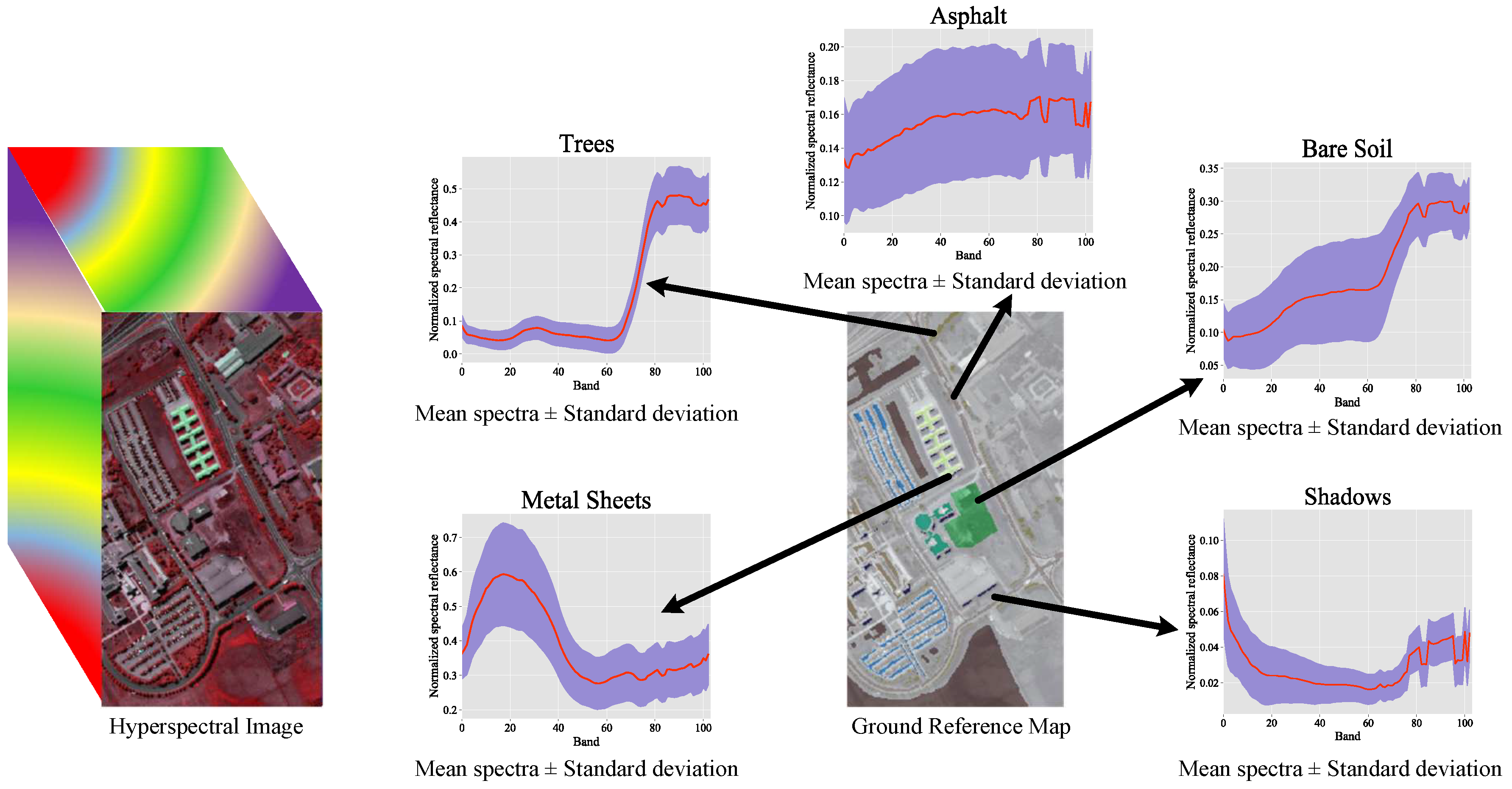
(1) UP: It was collected by the ROSIS sensor and contains 610 × 340 spectral samples with 103 bands. The spatial resolution is 1.3 m/pixel and the wavelength range of bands is between 0.43 and 0.86 μ m. The corresponding ground truth map consists of nine classes of land cover.
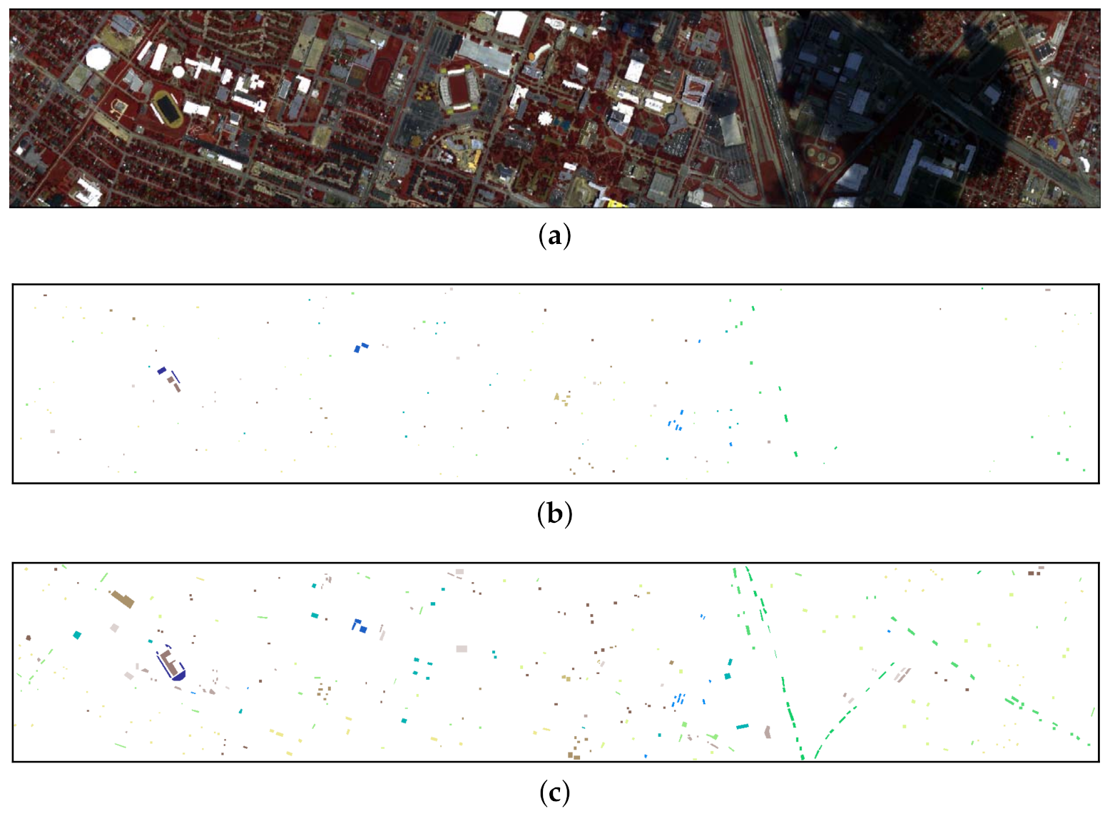
(2) UH: It was captured by the CASI sensor and has 349 × 1905 spectral samples with 144 bands. The spatial resolution is 2.5 m/pixel and the wavelength range of bands is between 0.38 and 1.05 μ m. The corresponding ground truth map consists of 15 classes of land cover.
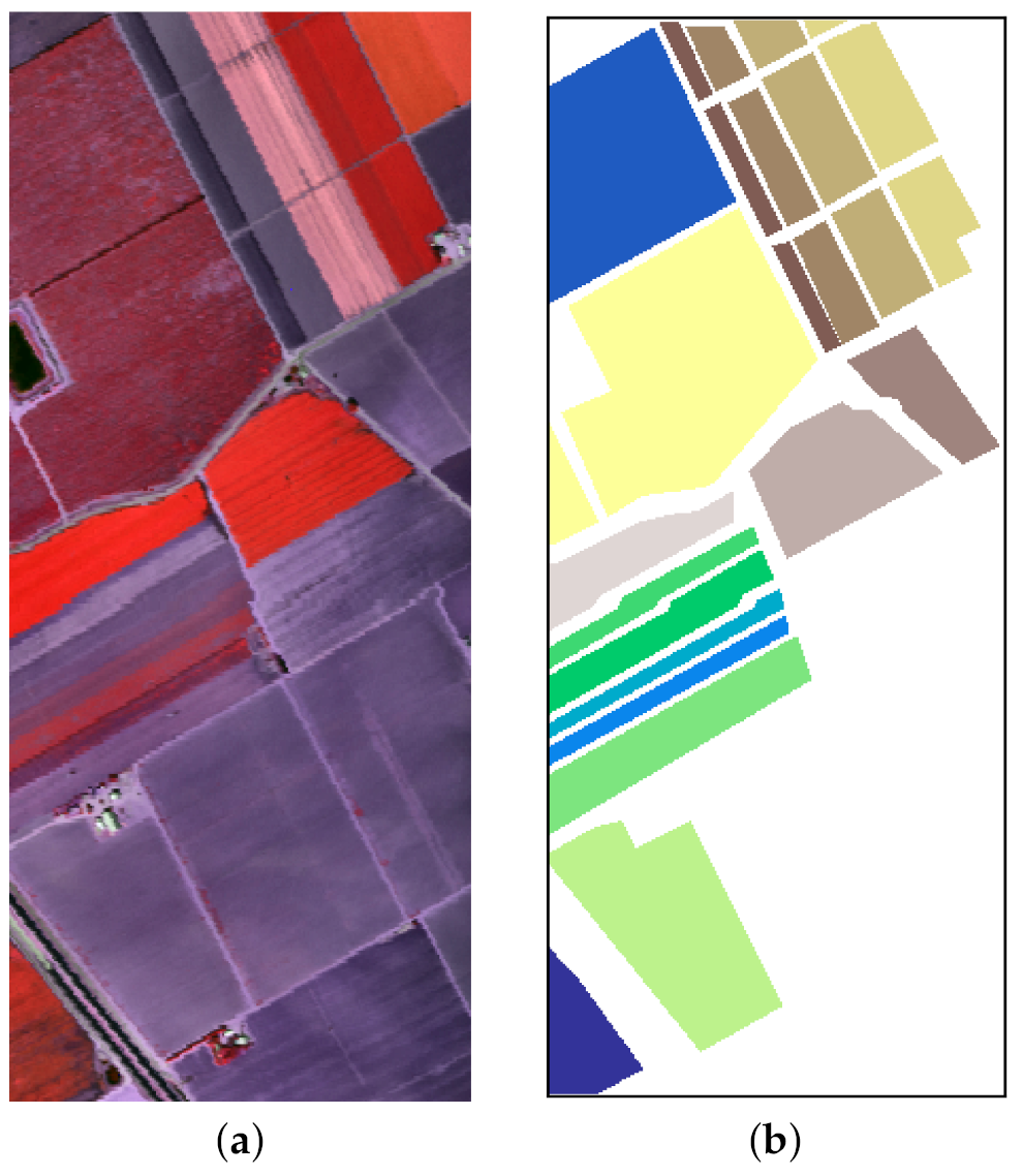
(3) SV: It was gathered by the AVIRIS sensor over Salinas Valley, CA, USA, containing 512 × 217 pixels and 204 available spectral bands. The wavelength range is between 0.4 and 2.5 μ m. The spatial resolution is 3.7 m/pixel. The corresponding ground truth map consists of 16 different land-cover classes.
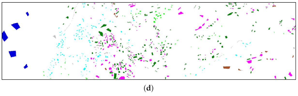
(4) HyRANK: The ISPRS HyRANK dataset is a recently released hyperspectral benchmark dataset. Different from the widely used hyperspectral benchmark datasets that consist of a single hyperspectral scene, the HyRANK dataset comprises two hyperspectral scenes, namely Dioni and Loukia. The available labeled samples in the Dioni scene are used for training, while those in the Loukia scene are used for test. The Dioni and Loukia scenes comprise 250 × 1376 and 249 × 945 spectral samples, respectively, and they have the same number of spectral reflectance bands, i.e., 176.
Note that the widespread random sampling strategy overlooks the spatial dependence between training and test samples, which usually leads to information leakage (i.e., overlap between the training and test HSI patches) and overoptimistic results when performing spectral-spatial classification [65]. To reduce the overlap and select spatially separated samples, researchers propose using spatially disjoint training and test sets to evaluate the HSI classification performance [66,67].
For the UP, UH, and HyRANK datasets, the official disjoint training and test sets were considered. The standard fixed training and test sets for the UP scene are available at: http://dase.grss-ieee.org (accessed on 3 June 2021). The UH dataset is available at: https://www.grss-ieee.org/resources/tutorials/data-fusion-tutorial-in-spanish/ (accessed on 3 June 2021). The HyRANK dataset is available at https://www2.isprs.org/commissions/comm3/wg4/hyrank/ (accessed on 3 June 2021). Taking the HyRANK dataset as an example, the available labeled samples in the Dioni scene are used for training, while those in the Loukia scene are used for test. Therefore, there is no information leakage between the patches contained within the training and test sets. Since the spatial distribution of the training and test samples is fixed for these three datasets, we executed our experiments five times over the same split, in order to avoid the influence of random initialization of network parameters on its performance.
For the SV dataset, since it does not have official spatially disjoint training and test sets, we first randomly selected 30 samples from each class in the ground truth for network training, and the remaining were used for test. Table 2, Table 3, Table 4 and Table 5 summarize the detail information of each category in these four datasets. Figure 8, Figure 9, Figure 10 and Figure 11 show the false color image and the distribution of available labeled samples of the four hyperspectral scenes.
The classification performance of all approaches was evaluated quantitatively with per-class classification accuracy, overall classification accuracy (OA), average classification accuracy (AA), and kappa coefficients ( κ ).

4.2. Parameters Analysis

The classification performance of our DRIN is affected by the parameter selection to a certain extent. We therefore experimentally analyzed the influences of some main parameters involved in the proposed network for the optimal results, including the involution kernel size, the reduction ratio r, and the group number G. 
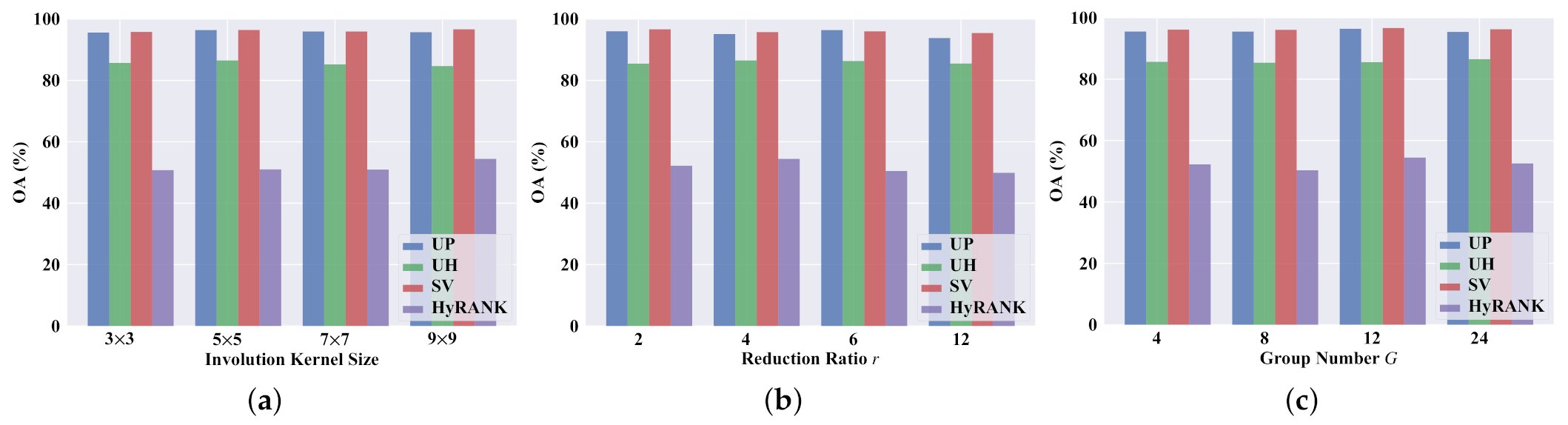
Figure 12 presents the resulting quantitative results (in terms of OA).
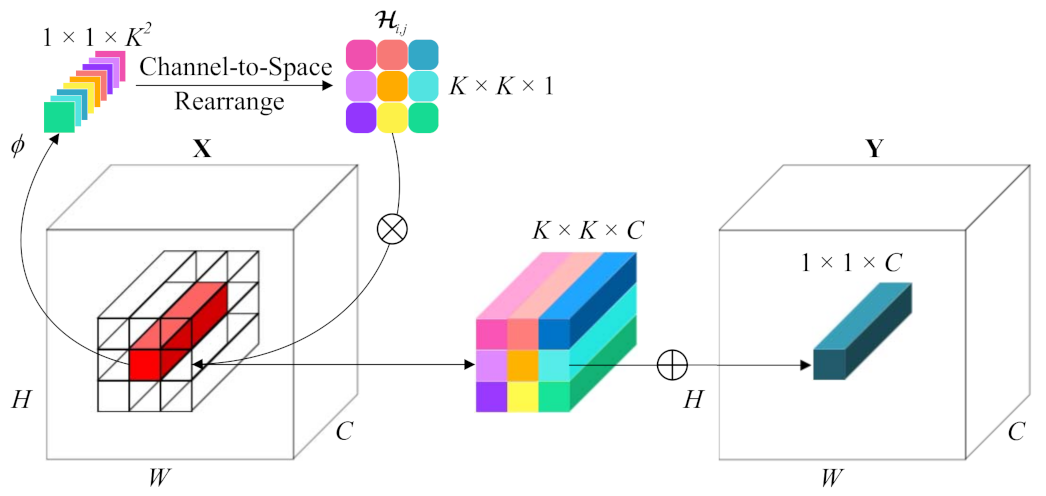
When employing a larger involution kernel, the proposed DRIN could utilize spatial context information in a wider spatial arrangement, capturing long-range spatial dependencies for correctly identifying the land cover type of each pixel. To prove this benefit, DRINs with different sizes of involution kernel (i.e., 3 × 3 , 5 × 5 , 7 × 7 , and 9 × 9 ) were implemented, and the obtained results are shown in Figure 12a. As can be seen, the best OA values are achieved when the involution kernel size is set to 5 × 5 , 5 × 5 , 9 × 9 , and 9 × 9 for the UP, UH, SV, and HyRANK datasets, respectively, which suggests that utilizing a larger involution kernel is helpful for increasing the classification accuracy. Note that the UP and UH scenes have more detailed regions, thus considering too large spatial context could weaken the information of the target pixel. As for the SV and HyRANK scenes, since they have larger smooth regions, dynamically reasoning in an enlarged spatial range could capture long-range dependencies well and hence offer better classification performance.
Reduction ratio 
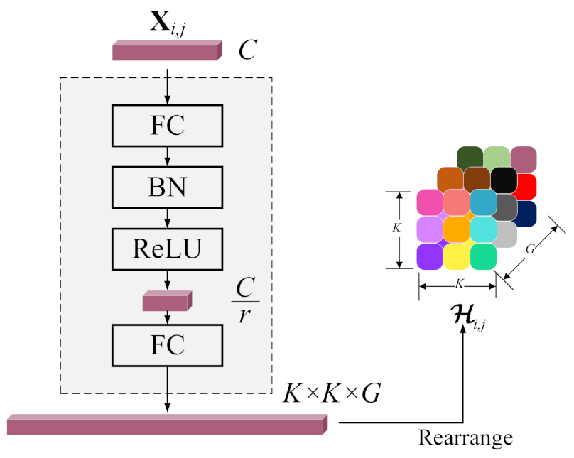
r controls the intermediate channel dimension between the two linear transformations in the kernel generation function ϕ . Specifically, appropriate parameter r could reduce the parameter count and permit the usage of larger involution kernel size under the same budget. Figure 12b illustrates the influence of different values of reduction ratio r on the OA of the our DRIN. For different datasets, the degree of influence and the optimal value are different. Based on the classification outcomes, the optimum values of reduction ratio r for the UP, UH, SV, and HyRANK datasets are 6, 4, 2, and 4, respectively.
Group number G is also a crucial factor in feature representation of DRIN. The more groups there are, the more distinct involution kernels are involved for discriminative spatial feature extraction. We select the optimum group number G from {4, 8, 12, 24} for each dataset. As shown in Figure 12c, the proposed DRIN with G = 12 achieves the highest OA on the UP, SV, and HyRANK datasets, and the best performance is obtained when G = 24 on the UH dataset. As a result, to obtain the optimal results, the G is set to 12, 24, 12, and 12 for the four datasets, respectively.
Taking the HyRANK dataset as an example, the influence of these three hyperparameters on the number of parameters and the computational complexity (in terms of the number of multiply-accumulate operations (MACs)) was further analyzed. Table 6, Table 7 and Table 8 show the classification performance and the number of parameters and MACs of the proposed DRIN with different involution kernel sizes, G, and r on the HyRANK dataset, respectively. As can be seen in Table 6, increasing involution kernel size can improve the classification accuracies. Note that the parameter count of convolution kernels increases quadratically with the increase of the kernel size. However, for the involution operation, we can harness large kernel while avoid introducing too many extra parameters. In addition, we adopt a bottleneck architecture to achieve efficient kernel generation. As shown in Table 7, although aggressive channel reduction ( r = 12 ) significantly reduces the number of parameters and MACs, it harms the classification performance (i.e., the lowest OA score of 49.9% is obtained). As long as r is set to an acceptable range, the proposed DRIN not only obtains good performance but also reduces the parameter count and computational cost. In addition, for the proposed DRIN, we share the involution kernels across different channels to reduce the parameter count and computational cost. The smaller is the G, the more channels share the same involution kernels. As shown in Table 8, the non-shared DRIN ( G = 24 ) incurs more parameters and MACs, while obtaining the second best OA score. The possible reason of this phenomenon is that the limited training samples in the HSI classification task are not enough to train networks with excessive parameters.

4.3. Classification Results

The proposed DRIN was compared with two traditional machine learning methods, namely, SVM [11] and extended morphological profiles (EMP) [8], and seven convolution-based networks, namely, deep&dense CNN (DenseNet) [57], deep pyramidal residual network (DPRN) [55], fully dense multiscale fusion network (FDMFN) [58], multiscale residual network with mixed depthwise convolution (MSRN) [32], lightweight spectral-spatial convolution module-based residual network (LWRN) [34], spatial-spectral squeeze-and-excitation residual network (SSSERN) [60], and deep residual network (DRN) [64].
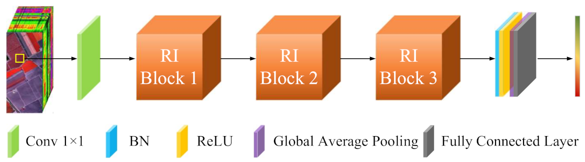
DRN and the proposed DRIN have a similar architecture. The DRN is regarded as a baseline model and can be obtained by replacing all involution layers in the DRIN with the standard 3 × 3 Conv layer. For all network models, the input patch size was fixed to be 11 × 11 to make a fair comparison. All the network models were implemented with the deep-learning framework of PyTorch and accelerated with an NVIDIA GeForce RTX 2080 GPU (with 8-GB GPU memory).
For the UP dataset, the proposed DRIN achieves the highest OA, as shown in Table 9. To be specific, the OA obtained by our DRIN is 96.4%, which is higher than that of SVM (80.0%), EMP (83.2%), DenseNet (91.6%), DPRN (92.1%), FDMFN (92.8%), MSRN (90.6%), LWRN (93.4%), SSSERN (94.4%), and its convolution-based counterpart DRN (95.9%). In comparison with the traditional machine learning approaches, SVM and EMP, the proposed network significantly increases the OA by 16.4% and 13.2%, respectively. In addition, compared with the DenseNet, DPRN, FDMFN, MSRN, LWRN, SSSERN, and DRN, the improvements in κ achieved by the proposed DRIN are 6.7%, 6.0%, 4.9%, 8.1%, 4.2%, 2.7%, and 0.6%, respectively.
Table 10 presents the classification results for the UH dataset. The proposed DRIN attains the highest overall metrics. Specifically, the OA, AA, and κ values are 86.5%, 88.6%, and 85.4%, respectively. In comparison with the second best approach, i.e., the MSRN, the performance improvements for OA, AA, and κ metrics are +0.6%, +0.5%, and +0.6%, respectively. The baseline model DRN is able to achieve satisfactory performance on this dataset. In comparison with it, the proposed involution-powered DRIN achieves higher OA, AA, and κ values, proving the superiority of larger dynamic involution kernel over compact and static 3 × 3 convolution kernel. To be specific, our proposed model improves OA, AA, and κ values from 85.2% to 86.5%, 87.5% to 88.6%, and 84.0% to 85.4%, respectively.
Table 11 reports the classification results for the SV dataset. SVM shows the worst performance and EMP is better than SVM. Thanks to the excellent nonlinear and hierarchical feature extraction ability, the other deep learning-based approaches, i.e., DenseNet, DPRN, FDMFN, MSRN, LWRN, SSSERN, DRN, and the proposed DRIN, outperform the SVM and EMP on the SV dataset. Specifically, compared to spectral classification approach SVM, DRIN significantly enhances OA and κ by about 10%. Besides, the proposed DRIN achieves 96.7% OA, 98.6% AA, and 96.3% κ , which are higher than those obtained by DRN. This again demonstrates the effectiveness and superiority of involution.
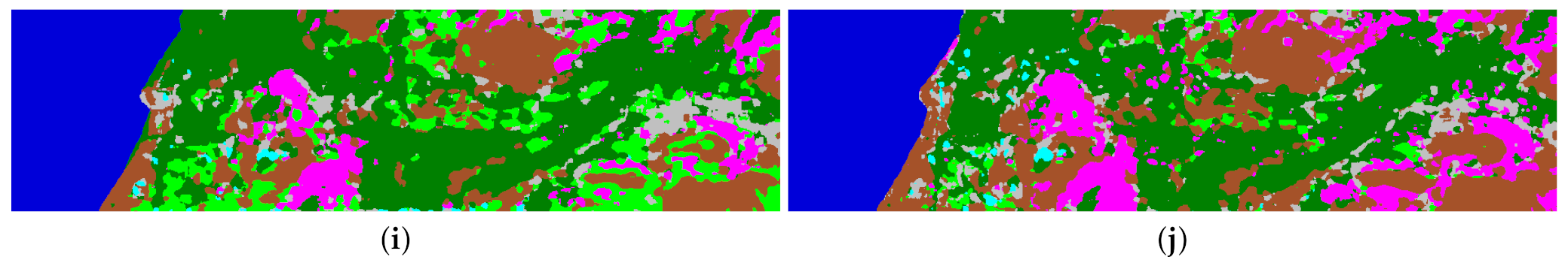
The classification accuracies of different approaches for the HyRANK dataset are summarized in Table 12, and the proposed DRIN achieves the highest overall accuracy among all the compared approaches. In comparison with DRN, our DRIN significantly increases the OA by 2.3%. In addition, the AA and κ values obtained by our DRIN are nearly 3% higher than those achieved by DRN. This experiment on the recently released HyRANK benchmark again verifies that the proposed involution-powered DRIN can achieve better classification performance than the convolutional baseline DRN.
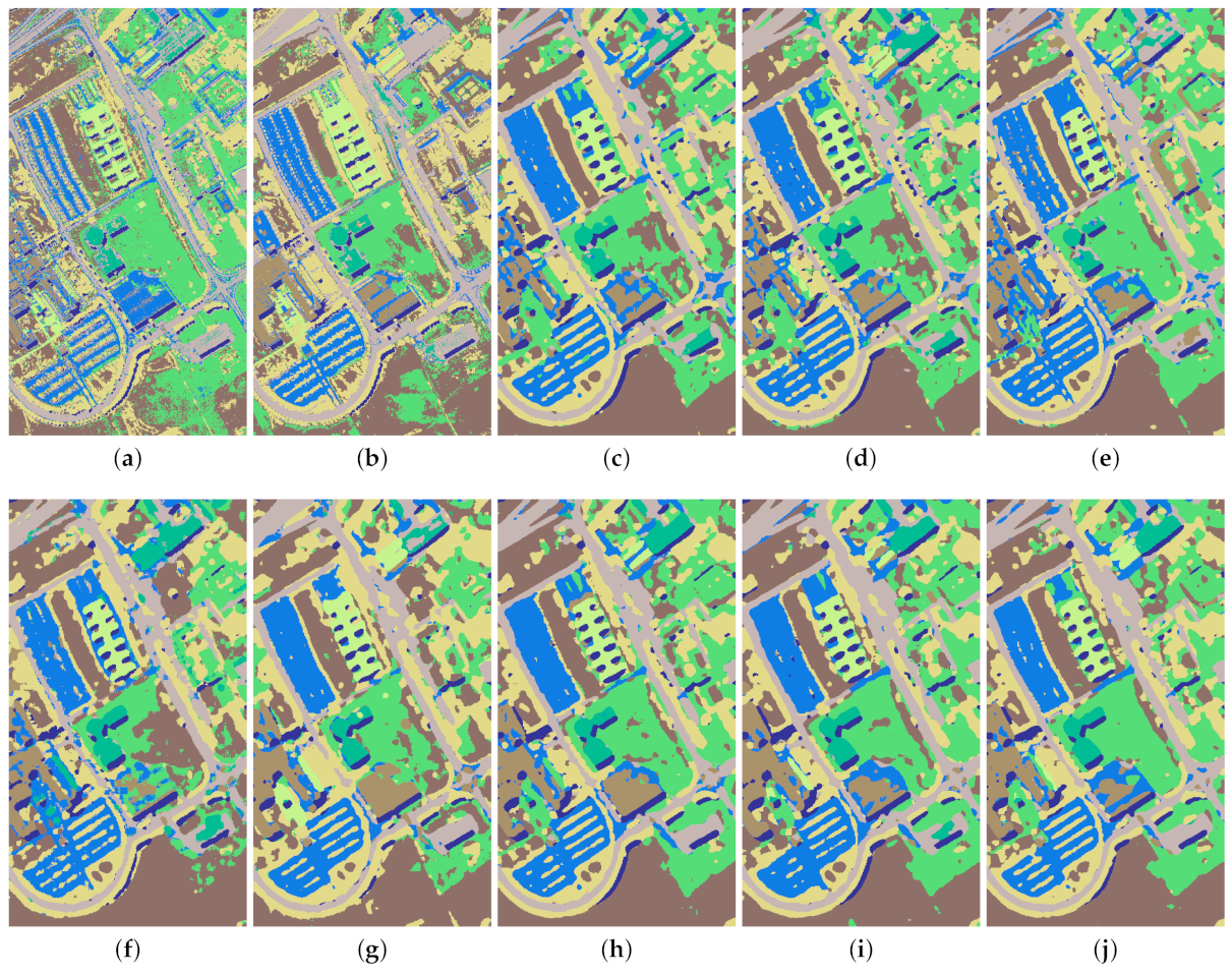
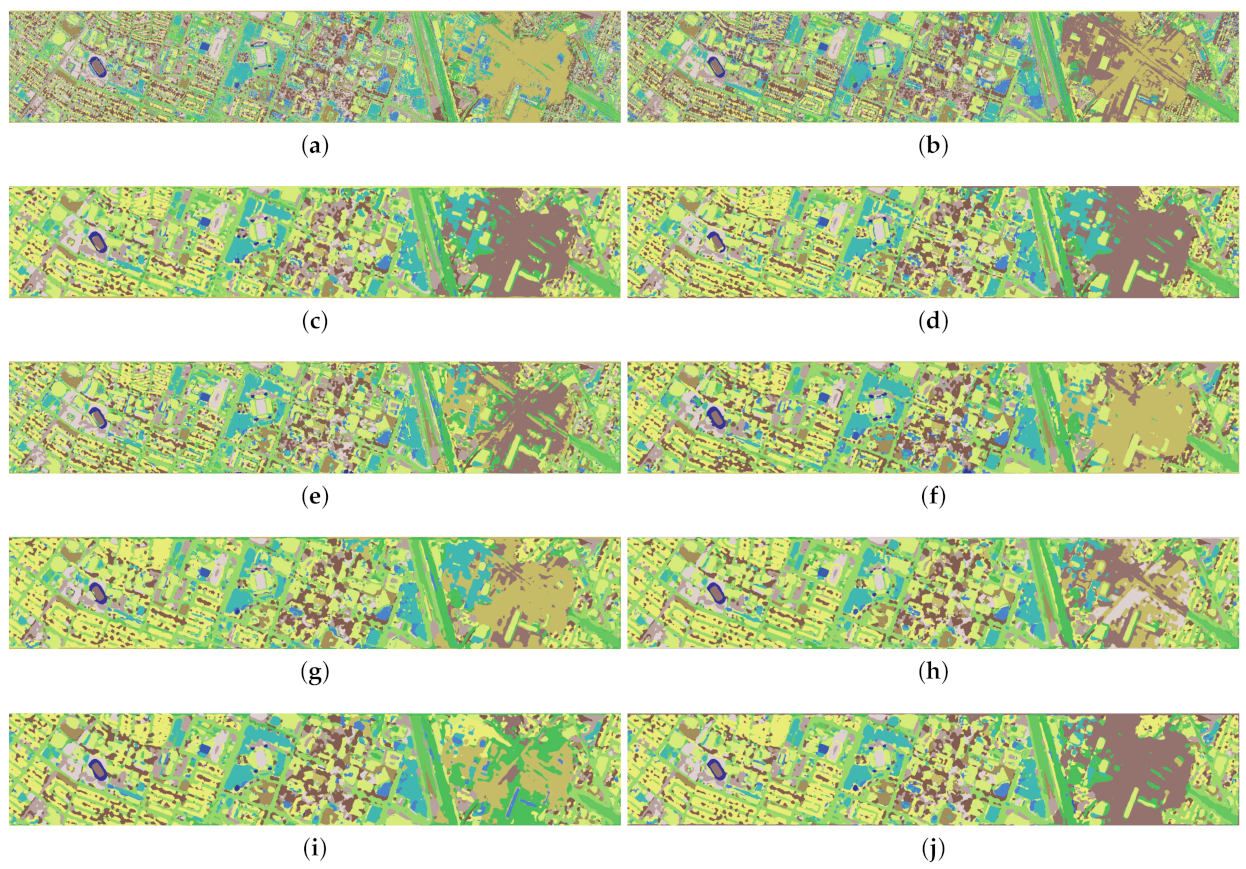
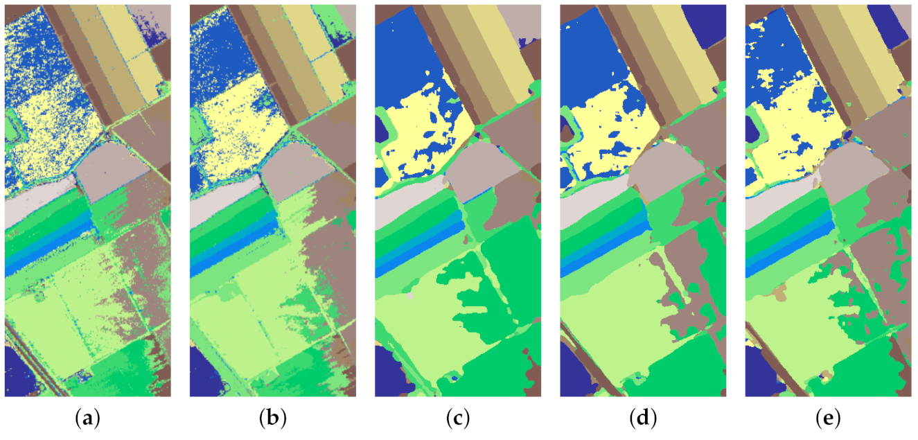
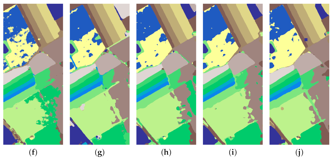
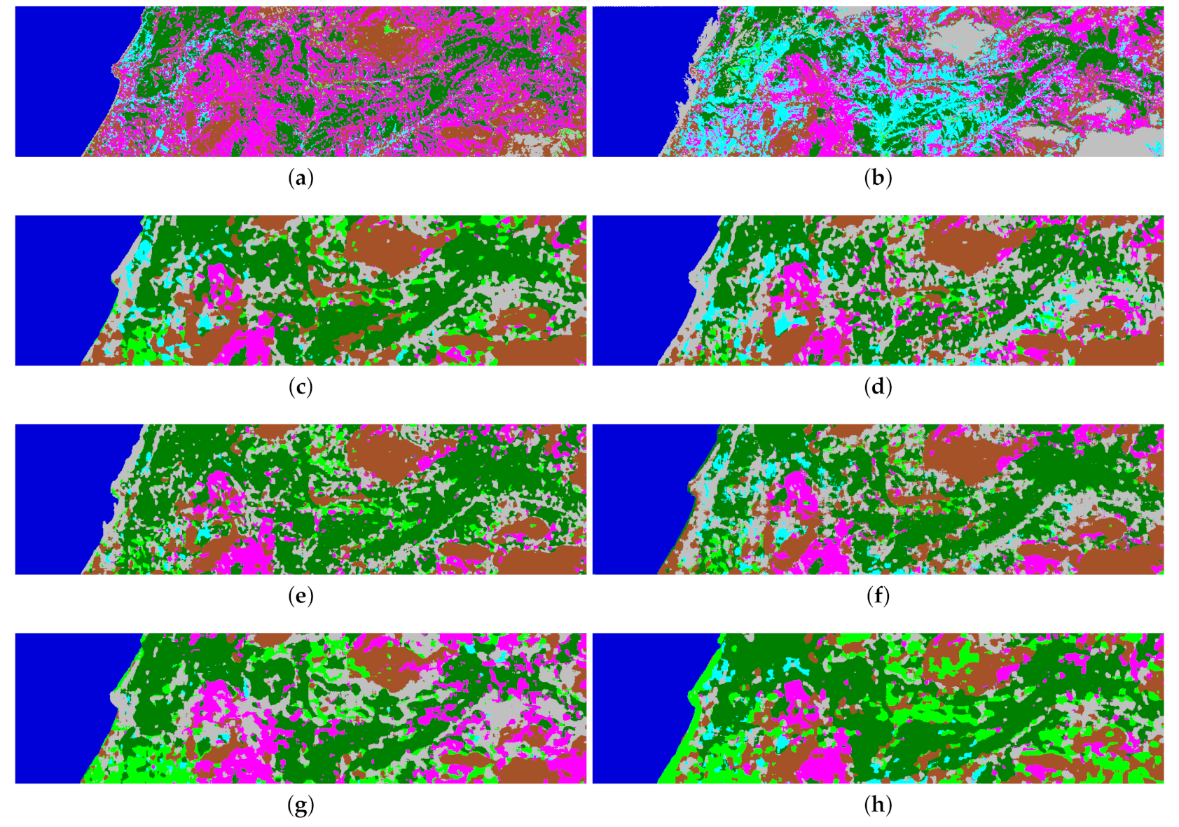
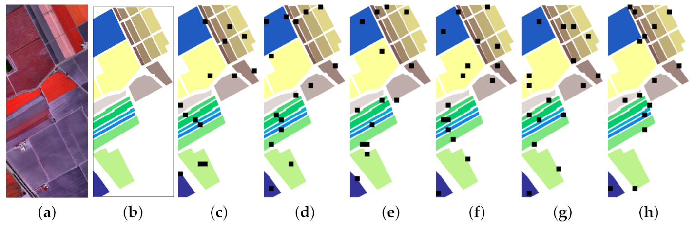
The classification maps of different approaches are illustrated in Figure 13, Figure 14, Figure 15 and Figure 16. Taking the SV dataset as an example, it is obvious that the classification maps generated by the SVM and EMP present many noisy scatter points, while the other deep learning-based methods mitigate this problem through the elimination of noisy scattered points of misclassification (see Figure 15). Clearly, our DRIN’s classification map is close to the ground truth map (see Figure 10b), especially in the region of grapes-untrained (Class 8). This is in consistent with the quantitative results reported in Table 11, where our DRIN model achieves the highest classification accuracy of 88.7% for the grapes-untrained category.
Focusing on the obtained overall classification accuracies, the proposed involution-based DRIN model consistently outperforms its convolution-based counterpart DRN on the four datasets. Specifically, in comparison with DRN, the proposed network increases the OA by 0.5%, 1.3%, 0.4%, and 2.3% on the UP, UH, SV, and HyRANK datasets, respectively, demonstrating the effectiveness of our DRIN model. 
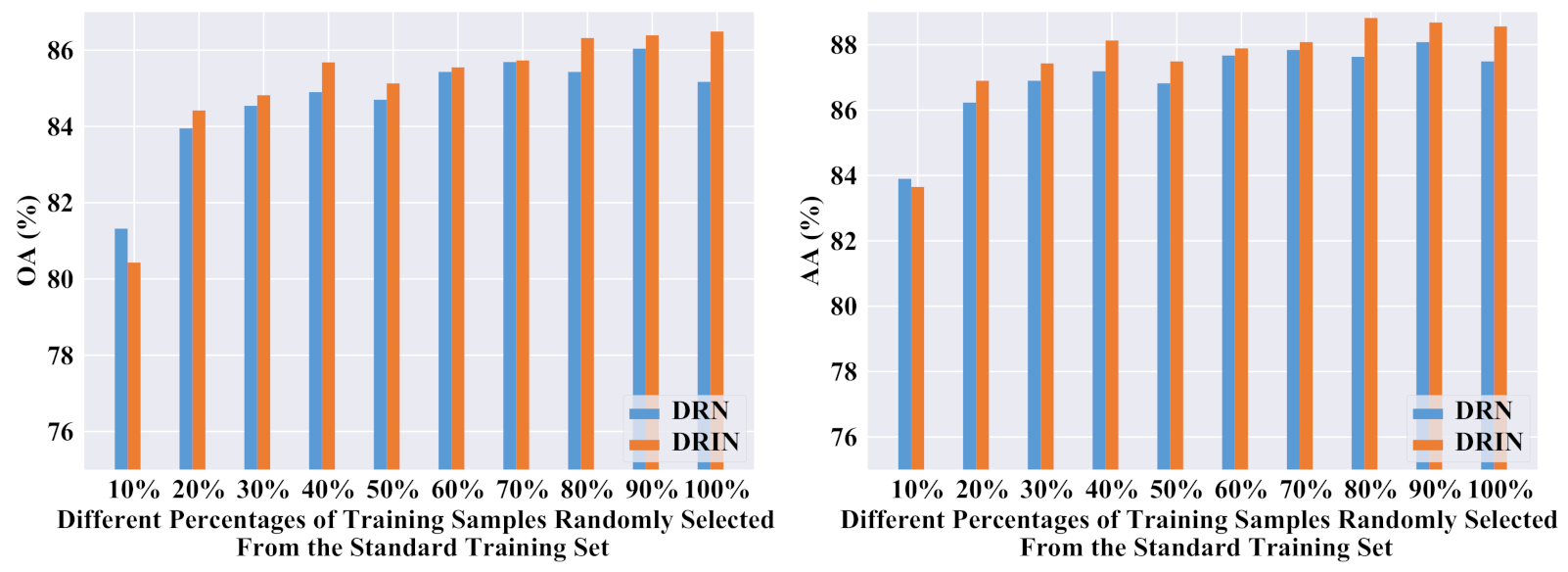
Figure 17 further shows the classification results when different number of samples are used for training on the UH dataset. It is apparent that DRIN is better than DRN in most cases.
In addition, our proposed DRIN could deliver enhanced performance at reduced parameter count compared to its counterpart DRN. Table 13 gives information about the OA and the corresponding model parameters. Specifically, for the UP dataset, DRIN is able to achieve a margin of 0.5% higher OA over DRN, using 26.07% fewer parameters. For the UH dataset, the proposed DRIN significantly increases the OA by 1.3% as compared with the DRN model, while requiring fewer parameters. For the SV dataset, the proposed DRIN with 3 × 3 involution kernel (denoted as DRIN*) can also obtain higher OA than DRN, with 23.27% fewer parameters. As for the HyRANK dataset, the proposed DRIN* with 14,430 fewer parameters can obtain 1.0% gains in terms of OA as compared with DRN. Moreover, with only 5328 more parameters, the OA of the proposed DRIN is 2.3% better than that of DRN.
Regarding the runtimes, the proposed DRIN consumes more time than the DRN. Taking the UP data set as an example, the running time of the DRN is 119.54 s, while the proposed DRIN consumes 183.19 s. The reason behind this is that the convolution layer is trained more efficiently than involution layer on GPU. In the future, a customized CUDA kernel implementation of the involution operation will be explored, to efficiently utilize computational hardware (i.e., GPU) and reduce the time cost.
To understand the contributions of the proposed DRIN’s two core components, residual learning and involution operation, we further constructed a plain CNN model (without residual learning) for comparison, which is obtained by eliminating the skip connections from the DRN model. The classification results obtained by CNN, DRN, and DRIN are summarized in Table 14. Note that, for a fair comparison, these three networks have the same number of layers and are trained under exactly the same experimental setting. As can be seen in Table 14, in comparison with the CNN, the performance improvements (in term of OA) obtained by DRN are +2.1%, +3.0%, +0.4%, and +2.1% on the UP, UH, SV, and HyRANK datasets, respectively, which demonstrate that residual learning plays a positive role in enhancing the HSI classification performance. Compared with DRN, the proposed involution-powered DRIN model further increases the OA by +0.5%, +1.3%, +0.4%, and +2.3% on the four datasets, which shows that the involution operation is also useful to improve the HSI classification accuracy. As can be seen, the improvement achieved by residual learning technique outperforms that obtained by the involution operation on the UP and UH datasets. However, compared with DRN, the proposed involution-powered DRIN can significantly increase the OA by +1.3% and +2.3% on the UH and HyRANK datasets, respectively, which demonstrates the huge potential of designing involution-based networks. More importantly, our DRIN model using both techniques performs the best on all four HSI datasets, demonstrating its effectiveness for HSI classification.
In addition, considering that the random sampling strategy usually leads to overoptimistic results, we further compared the proposed DRIN with other deep models on the SV dataset using spatially disjoint training and test samples. We used a novel sampling strategy [65] to select training and test samples, which can avoid the overlap between the training and test sets and hence the information leakage. We extracted six-fold training–test splits for cross validation (see Figure 18) and repeated the experiments five times for each fold. Therefore, we performed 30 independent Monte Carlo runs for the proposed DRIN and the overall classification accuracies are reported. In this experiment, the proportion of training samples in each fold is about 3%, and the training HSI patches can only be selected within the black area, as shown in Figure 18. For more details of this sampling strategy, please refer to the work of Nalepa et al. [65]. As shown in Table 15, the proposed DRIN again achieves better performance over the other compared approaches. In addition, we further analyzed the influence of involution kernel size on the classification performance using these six non-overlapping training–test splits. The experimental results are summarized in Table 16. We can easily observe that using a larger involution kernel could deliver improvements in accuracy.
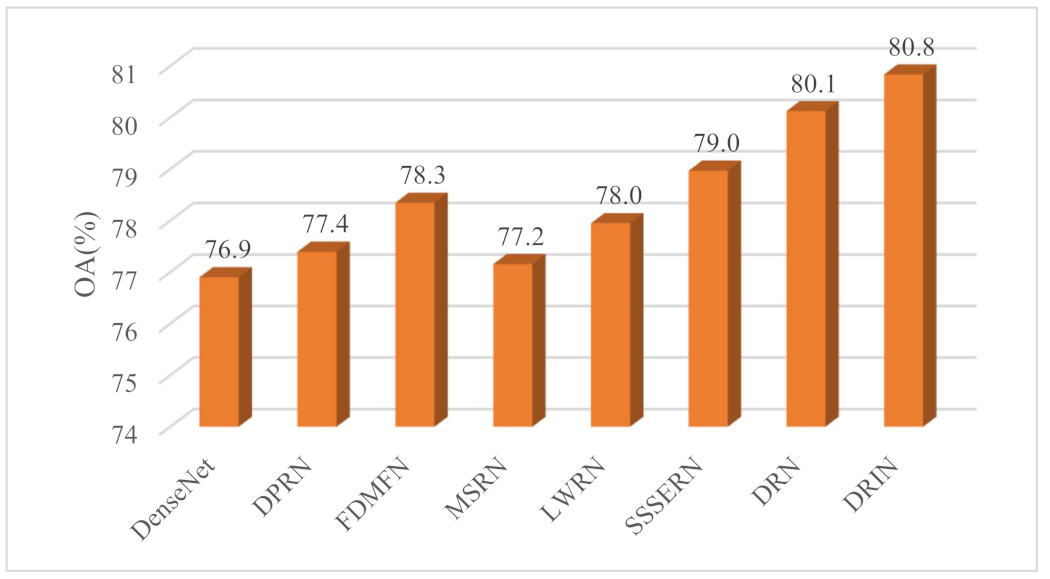
In summary, extensive experimental results on four benchmark datasets demonstrate that employing DRIN could deliver very promising results in terms of increasing classification accuracy and reducing model parameters. In addition, in order to present a global view of the classification performance of the compared deep models, the aggregated results across all four benchmarks are presented. Specifically, we average the OA scores obtained by different deep models on the four HSI datasets. As can be seen in Figure 19, the proposed DRIN achieves the highest averaged OA score (i.e., 80.8%). Besides, to verify the importance of the differences across different CNN models, we executed Wilcoxon signed-rank tests over OA. As can be observed in Table 17, the differences between the proposed DRIN and other models are statistically important. For instance, the proposed DRIN delivers significant improvements over DRN in accuracy, according to the Wilcoxon tests at p < 0.005 .

5. Discussion

Different from the convolution operation, the involution operation can adaptively allocate weights over different spatial positions. To verify the effectiveness of the dynamic involution operation, we further compared the proposed DRIN with the baseline DRN model that uses the same size of the static convolution kernel for spatial feature learning. As shown in Table 18, the proposed DRIN consistently achieves better performance than DRN while containing fewer parameters, again demonstrating the effectiveness and efficiency of the proposed spectral feature-based dynamic involution kernel. Taking the HyRANK dataset as an example, the proposed DRIN is able to achieve 3.5% higher OA over DRN while using 3.23× fewer parameters.
Note that the spectral feature-based involution kernels used in the proposed DRIN are distinct over different spatial positions (i.e., spatial specific), which could prioritize the informative visual elements. For each involution kernel, the sum of the K × K kernel weights can be taken as its representative value [41]. By plotting the representative values at diverse spatial positions, we can frame a heat map to dissect the learned involution kernels. Figure 20 shows the heat maps of the involution kernels learned in the third RI block, separated by groups. As can be seen, different kernels automatically attend to varying semantic concepts for correct pixel recognition. For example, sharp edges or corners, the outlines of different objects, smoother regions, and peripheral parts are highlighted in different heat maps.
In addition, the enlarged involution kernel could capture long-range spatial interactions, which enhances the utilization of the key spatial context information for target pixel recognition. Moreover, each involution kernel corresponds to an individual feature channel (similar to the depthwise convolution operation [68]) and different channels could share the same kernel, which enables the involution operation to be implemented in a fairly lightweight manner. Therefore, our proposed involution-based DRIN model could achieve better classification performance than its convolution-based counterpart with fewer parameters.

6. Conclusions

In this paper, an involution-powered network, DRIN, is proposed for HSI classification. As a notable characteristic, the proposed DRIN could capture long-range spatial interactions through harnessing large involution kernels, while avoiding prohibitive memory consumption. Moreover, the dynamically parameterized involution kernel could adapt to different visual patterns with respect to diverse spatial locations. Experiments conducted on four benchmark datasets demonstrate that DRIN not only offers better performance than the convolution-based counterparts but also outperforms other state-of-the-art HSI classification algorithms.
Future work can be devoted to exploring more exquisite kernel generation functions for enhancing the discriminative feature learning ability of the involution kernel. In addition, we believe that exploring more effective involution-equipped neural networks will aid future research for accurate HSI classification.

Author Contributions

Conceptualization, Z.M.; methodology, Z.M.; software, Z.M.; writing—original draft preparation, Z.M.; writing—review and editing, Z.M.; funding acquisition, F.Z., M.L. and W.X. All authors have read and agreed to the published version of the manuscript.

Funding

This research was funded by the National Natural Science Foundation of China under Grants 61901198, 62071378, and 62071379; in part by the Scientific Research Program Funded by Shaanxi Provincial Education Department under Grant 20JK0904; in part by the Natural Science Basic Research Plan in Shaanxi Province of China under Grant 2021JM-461; in part by the Program of Qingjiang Excellent Young Talents, Jiangxi University of Science and Technology under Grant JXUSTQJYX2020019; in part by the New Star Team of Xi’an University of Posts & Telecommunications under Grant xyt2016-01.

Institutional Review Board Statement

Not applicable.

Informed Consent Statement

Not applicable.

Data Availability Statement

The standard training and test sets for the UP scene are available at: http://dase.grss-ieee.org, accessed on 3 June 2021. The UH scene is available at: https://www.grss-ieee.org/resources/tutorials/data-fusion-tutorial-in-spanish/, accessed on 3 June 2021. The SV scene is available at: http://www.ehu.eus/ccwintco/index.php?title=Hyperspectral_Remote_Sensing_Scenes, accessed on 3 June 2021. The HyRANK dataset is available at https://www2.isprs.org/commissions/comm3/wg4/hyrank/, accessed on 3 June 2021.

Acknowledgments

The authors would like to thank the Assistant Editor and the anonymous reviewers for providing truly outstanding comments and suggestions that significantly helped us improve the technical quality and presentation of our paper.

Conflicts of Interest

The authors declare no conflict of interest.

References

  1. Kirsch, M.; Lorenz, S.; Zimmermann, R.; Tusa, L.; Möckel, R.; Hödl, P.; Booysen, R.; Khodadadzadeh, M.; Gloaguen, R. Integration of terrestrial and drone-borne hyperspectral and photogrammetric sensing methods for exploration mapping and mining monitoring. Remote Sens. 2018, 10, 1366. [Google Scholar] [CrossRef] [Green Version]
  2. Van Der Meer, F. Analysis of spectral absorption features in hyperspectral imagery. Int. J. Appl. Earth Obs. Geoinform. 2004, 5, 55–68. [Google Scholar] [CrossRef]
  3. Zhong, Y.; Hu, X.; Luo, C.; Wang, X.; Zhao, J.; Zhang, L. WHU-Hi: UAV-borne hyperspdectral with high spatial resolution (H2) benchmark datasets and classifier for precise crop identification based on deep convolutional neural network with CRF. Remote Sens. Environ. 2020, 250, 112012. [Google Scholar] [CrossRef]
  4. Stuart, M.B.; McGonigle, A.J.; Willmott, J.R. Hyperspectral imaging in environmental monitoring: A review of recent developments and technological advances in compact field deployable systems. Sensors 2019, 19, 3071. [Google Scholar] [CrossRef] [Green Version]
  5. Hao, S.; Wang, W.; Ye, Y.; Nie, T.; Bruzzone, L. Two-stream deep architecture for hyperspectral image classification. IEEE Trans. Geosci. Remote Sens. 2017, 56, 2349–2361. [Google Scholar] [CrossRef]
  6. Mou, L.; Zhu, X.X. Learning to pay attention on spectral domain: A spectral attention module-based convolutional network for hyperspectral image classification. IEEE Trans. Geosci. Remote Sens. 2019, 58, 110–122. [Google Scholar] [CrossRef]
  7. Hong, D.; Wu, X.; Ghamisi, P.; Chanussot, J.; Yokoya, N.; Zhu, X.X. Invariant attribute profiles: A spatial-frequency joint feature extractor for hyperspectral image classification. IEEE Trans. Geosci. Remote Sens. 2020, 58, 3791–3808. [Google Scholar] [CrossRef] [Green Version]
  8. Benediktsson, J.A.; Palmason, J.A.; Sveinsson, J.R. Classification of hyperspectral data from urban areas based on extended morphological profiles. IEEE Trans. Geosci. Remote Sens. 2005, 43, 480–491. [Google Scholar] [CrossRef]
  9. Li, W.; Chen, C.; Su, H.; Du, Q. Local binary patterns and extreme learning machine for hyperspectral imagery classification. IEEE Trans. Geosci. Remote Sens. 2015, 53, 3681–3693. [Google Scholar] [CrossRef]
  10. Melgani, F.; Bruzzone, L. Classification of hyperspectral remote sensing images with support vector machines. IEEE Trans. Geosci. Remote Sens. 2004, 42, 1778–1790. [Google Scholar] [CrossRef] [Green Version]
  11. Waske, B.; van der Linden, S.; Benediktsson, J.A.; Rabe, A.; Hostert, P. Sensitivity of support vector machines to random feature selection in classification of hyperspectral data. IEEE Trans. Geosci. Remote Sens. 2010, 48, 2880–2889. [Google Scholar] [CrossRef] [Green Version]
  12. Li, S.; Song, W.; Fang, L.; Chen, Y.; Ghamisi, P.; Benediktsson, J.A. Deep learning for hyperspectral image classification: An overview. IEEE Trans. Geosci. Remote Sens. 2019, 57, 6690–6709. [Google Scholar] [CrossRef] [Green Version]
  13. Chen, Y.; Lin, Z.; Zhao, X.; Wang, G.; Gu, Y. Deep learning-based classification of hyperspectral data. IEEE J. Sel. Top. Appl. Earth Obs. Remote Sens. 2014, 7, 2094–2107. [Google Scholar] [CrossRef]
  14. Chen, Y.; Jiang, H.; Li, C.; Jia, X.; Ghamisi, P. Deep feature extraction and classification of hyperspectral images based on convolutional neural networks. IEEE Trans. Geosci. Remote Sens. 2016, 54, 6232–6251. [Google Scholar] [CrossRef] [Green Version]
  15. Zheng, Z.; Zhong, Y.; Ma, A.; Zhang, L. FPGA: Fast patch-free global learning framework for fully end-to-end hyperspectral image classification. IEEE Trans. Geosci. Remote Sens. 2020, 58, 5612–5626. [Google Scholar] [CrossRef]
  16. Tang, X.; Meng, F.; Zhang, X.; Cheung, Y.M.; Ma, J.; Liu, F.; Jiao, L. Hyperspectral image classification based on 3-D octave convolution with spatial-spectral attention network. IEEE Trans. Geosci. Remote Sens. 2021, 59, 2430–2447. [Google Scholar] [CrossRef]
  17. Meng, Z.; Jiao, L.; Liang, M.; Zhao, F. Hyperspectral image classification with mixed link networks. IEEE J. Sel. Top. Appl. Earth Obs. Remote Sens. 2021, 14, 2494–2507. [Google Scholar] [CrossRef]
  18. Chen, Y.; Zhao, X.; Jia, X. Spectral–spatial classification of hyperspectral data based on deep belief network. IEEE J. Sel. Top. Appl. Earth Obs. Remote Sens. 2015, 8, 2381–2392. [Google Scholar] [CrossRef]
  19. Mou, L.; Ghamisi, P.; Zhu, X.X. Deep recurrent neural networks for hyperspectral image classification. IEEE Trans. Geosci. Remote Sens. 2017, 55, 3639–3655. [Google Scholar] [CrossRef] [Green Version]
  20. Hang, R.; Liu, Q.; Hong, D.; Ghamisi, P. Cascaded recurrent neural networks for hyperspectral image classification. IEEE Trans. Geosci. Remote Sens. 2019, 57, 5384–5394. [Google Scholar] [CrossRef] [Green Version]
  21. Paoletti, M.E.; Haut, J.M.; Fernandez-Beltran, R.; Plaza, J.; Plaza, A.; Li, J.; Pla, F. Capsule networks for hyperspectral image classification. IEEE Trans. Geosci. Remote Sens. 2018, 57, 2145–2160. [Google Scholar] [CrossRef]
  22. Zhu, K.; Chen, Y.; Ghamisi, P.; Jia, X.; Benediktsson, J.A. Deep convolutional capsule network for hyperspectral image spectral and spectral-spatial classification. Remote Sens. 2019, 11, 223. [Google Scholar] [CrossRef] [Green Version]
  23. Wan, S.; Gong, C.; Zhong, P.; Du, B.; Zhang, L.; Yang, J. Multiscale dynamic graph convolutional network for hyperspectral image classification. IEEE Trans. Geosci. Remote Sens. 2019, 58, 3162–3177. [Google Scholar] [CrossRef] [Green Version]
  24. Hong, D.; Gao, L.; Yao, J.; Zhang, B.; Plaza, A.; Chanussot, J. Graph convolutional networks for hyperspectral image classification. IEEE Trans. Geosci. Remote Sens. 2020, 59, 5966–5978. [Google Scholar] [CrossRef]
  25. Zhu, L.; Chen, Y.; Ghamisi, P.; Benediktsson, J.A. Generative adversarial networks for hyperspectral image classification. IEEE Trans. Geosci. Remote Sens. 2018, 56, 5046–5063. [Google Scholar] [CrossRef]
  26. Feng, J.; Yu, H.; Wang, L.; Cao, X.; Zhang, X.; Jiao, L. Classification of hyperspectral images based on multiclass spatial–spectral generative adversarial networks. IEEE Trans. Geosci. Remote Sens. 2019, 57, 5329–5343. [Google Scholar] [CrossRef]
  27. He, J.; Zhao, L.; Yang, H.; Zhang, M.; Li, W. HSI-BERT: Hyperspectral image classification using the bidirectional encoder representation from transformers. IEEE Trans. Geosci. Remote Sens. 2019, 58, 165–178. [Google Scholar] [CrossRef]
  28. He, X.; Chen, Y.; Lin, Z. Spatial-spectral transformer for hyperspectral image classification. Remote Sens. 2021, 13, 498. [Google Scholar] [CrossRef]
  29. Li, Z.; Liu, M.; Chen, Y.; Xu, Y.; Li, W.; Du, Q. Deep cross-domain few-shot learning for hyperspectral image classification. IEEE Trans. Geosci. Remote Sens. 2021, 1–18. [Google Scholar] [CrossRef]
  30. Li, W.; Wu, G.; Zhang, F.; Du, Q. Hyperspectral image classification using deep pixel-pair features. IEEE Trans. Geosci. Remote Sens. 2016, 55, 844–853. [Google Scholar] [CrossRef]
  31. Fang, L.; Liu, G.; Li, S.; Ghamisi, P.; Benediktsson, J.A. Hyperspectral image classification with squeeze multibias network. IEEE Trans. Geosci. Remote Sens. 2019, 57, 1291–1301. [Google Scholar] [CrossRef]
  32. Gao, H.; Yang, Y.; Li, C.; Gao, L.; Zhang, B. Multiscale residual network with mixed depthwise convolution for hyperspectral image classification. IEEE Trans. Geosci. Remote Sens. 2021, 59, 3396–3408. [Google Scholar] [CrossRef]
  33. Paoletti, M.E.; Haut, J.M.; Pereira, N.S.; Plaza, J.; Plaza, A. Ghostnet for hyperspectral image classification. IEEE Trans. Geosci. Remote Sens. 2021, 1–16. [Google Scholar] [CrossRef]
  34. Meng, Z.; Jiao, L.; Liang, M.; Zhao, F. A lightweight spectral-spatial convolution module for hyperspectral image classification. IEEE Geosci. Remote Sens. Lett. 2021, 1–5. [Google Scholar] [CrossRef]
  35. Wang, C.; Zhang, L.; Wei, W.; Zhang, Y. Hyperspectral image classification with data augmentation and classifier fusion. IEEE Geosci. Remote Sens. Lett. 2019, 17, 1420–1424. [Google Scholar] [CrossRef]
  36. Acción, Á.; Argüello, F.; Heras, D.B. Dual-window superpixel data augmentation for hyperspectral image classification. Appl. Sci. 2020, 10, 8833. [Google Scholar] [CrossRef]
  37. Haut, J.M.; Paoletti, M.E.; Plaza, J.; Plaza, A.; Li, J. Hyperspectral image classification using random occlusion data augmentation. IEEE Geosci. Remote Sens. Lett. 2019, 16, 1751–1755. [Google Scholar] [CrossRef]
  38. Nalepa, J.; Myller, M.; Kawulok, M. Training-and test-time data augmentation for hyperspectral image segmentation. IEEE Geosci. Remote Sens. Lett. 2019, 17, 292–296. [Google Scholar] [CrossRef]
  39. Simonyan, K.; Zisserman, A. Very deep convolutional networks for large-scale image recognition. arXiv 2014, arXiv:1409.1556. [Google Scholar]
  40. Alipour-Fard, T.; Paoletti, M.; Haut, J.M.; Arefi, H.; Plaza, J.; Plaza, A. Multibranch selective kernel networks for hyperspectral image classification. IEEE Geosci. Remote Sens. Lett. 2020, 18, 1089–1093. [Google Scholar] [CrossRef]
  41. Li, D.; Hu, J.; Wang, C.; Li, X.; She, Q.; Zhu, L.; Zhang, T.; Chen, Q. Involution: Inverting the inherence of convolution for visual recognition. arXiv 2021, arXiv:2103.06255. [Google Scholar]
  42. Feng, J.; Liu, L.; Cao, X.; Jiao, L.; Sun, T.; Zhang, X. Marginal stacked autoencoder with adaptively-spatial regularization for hyperspectral image classification. IEEE J. Sel. Top. Appl. Earth Obs. Remote Sens. 2018, 11, 3297–3311. [Google Scholar] [CrossRef]
  43. Li, J.; Xi, B.; Li, Y.; Du, Q.; Wang, K. Hyperspectral classification based on texture feature enhancement and deep belief networks. Remote Sens. 2018, 10, 396. [Google Scholar] [CrossRef] [Green Version]
  44. Hu, W.; Huang, Y.; Wei, L.; Zhang, F.; Li, H. Deep convolutional neural networks for hyperspectral image classification. J. Sens. 2015, 2015, 258619. [Google Scholar] [CrossRef] [Green Version]
  45. Yue, J.; Zhao, W.; Mao, S.; Liu, H. Spectral–spatial classification of hyperspectral images using deep convolutional neural networks. Remote Sens. Lett. 2015, 6, 468–477. [Google Scholar] [CrossRef]
  46. Zhang, H.; Li, Y.; Zhang, Y.; Shen, Q. Spectral-spatial classification of hyperspectral imagery using a dual-channel convolutional neural network. Remote Sens. Lett. 2017, 8, 438–447. [Google Scholar] [CrossRef] [Green Version]
  47. Lorenzo, P.R.; Tulczyjew, L.; Marcinkiewicz, M.; Nalepa, J. Hyperspectral band selection using attention-based convolutional neural networks. IEEE Access 2020, 8, 42384–42403. [Google Scholar] [CrossRef]
  48. Zhang, H.; Lan, J.; Guo, Y. A dense spatial–spectral attention network for hyperspectral image band selection. Remote Sens. Lett. 2021, 1–13. [Google Scholar] [CrossRef]
  49. Zhang, H.; Li, Y.; Jiang, Y.; Wang, P.; Shen, Q.; Shen, C. Hyperspectral classification based on lightweight 3-D-CNN with transfer learning. IEEE Trans. Geosci. Remote Sens. 2019, 57, 5813–5828. [Google Scholar] [CrossRef] [Green Version]
  50. Zhu, J.; Fang, L.; Ghamisi, P. Deformable convolutional neural networks for hyperspectral image classification. IEEE Geosci. Remote Sens. Lett. 2018, 15, 1254–1258. [Google Scholar] [CrossRef]
  51. He, K.; Zhang, X.; Ren, S.; Sun, J. Deep residual learning for image recognition. In Proceedings of the IEEE Conference on Computer Vision and Pattern Recognition (CVPR), Las Vegas, NV, USA, 27–30 June 2016; pp. 770–778. [Google Scholar]
  52. Song, W.; Li, S.; Fang, L.; Lu, T. Hyperspectral image classification with deep feature fusion network. IEEE Trans. Geosci. Remote Sens. 2018, 56, 3173–3184. [Google Scholar] [CrossRef]
  53. Zhong, Z.; Li, J.; Luo, Z.; Chapman, M. Spectral–spatial residual network for hyperspectral image classification: A 3-D deep learning framework. IEEE Trans. Geosci. Remote Sens. 2017, 56, 847–858. [Google Scholar] [CrossRef]
  54. Meng, Z.; Li, L.; Tang, X.; Feng, Z.; Jiao, L.; Liang, M. Multipath residual network for spectral-spatial hyperspectral image classification. Remote Sens. 2019, 11, 1896. [Google Scholar] [CrossRef] [Green Version]
  55. Paoletti, M.E.; Haut, J.M.; Fernandez-Beltran, R.; Plaza, J.; Plaza, A.J.; Pla, F. Deep pyramidal residual networks for spectral–spatial hyperspectral image classification. IEEE Trans. Geosci. Remote Sens. 2019, 57, 740–754. [Google Scholar] [CrossRef]
  56. Huang, G.; Liu, Z.; Van Der Maaten, L.; Weinberger, K.Q. Densely connected convolutional networks. In Proceedings of the IEEE Conference on Computer Vision and Pattern Recognition (CVPR), Honolulu, HI, USA, 21–26 July 2017; pp. 4700–4708. [Google Scholar]
  57. Paoletti, M.E.; Haut, J.M.; Plaza, J.; Plaza, A. Deep&dense convolutional neural network for hyperspectral image classification. Remote Sens. 2018, 10, 1454. [Google Scholar]
  58. Meng, Z.; Li, L.; Jiao, L.; Feng, Z.; Tang, X.; Liang, M. Fully dense multiscale fusion network for hyperspectral image classification. Remote Sens. 2019, 11, 2718. [Google Scholar] [CrossRef] [Green Version]
  59. Kang, X.; Zhuo, B.; Duan, P. Dual-path network-based hyperspectral image classification. IEEE Geosci. Remote Sens. Lett. 2018, 16, 447–451. [Google Scholar] [CrossRef]
  60. Wang, L.; Peng, J.; Sun, W. Spatial–spectral squeeze-and-excitation residual network for hyperspectral image classification. Remote Sens. 2019, 11, 884. [Google Scholar] [CrossRef] [Green Version]
  61. Zhang, R. Making convolutional networks shift-invariant again. In Proceedings of the International Conference on Machine Learning (ICML), Los Angeles, CA, USA, 9–15 June 2019; pp. 7324–7334. [Google Scholar]
  62. Nie, J.; Xu, Q.; Pan, J.; Guo, M. Hyperspectral image classification based on multiscale spectral-spatial deformable network. IEEE Geosci. Remote Sens. Lett. 2020, 1–5. [Google Scholar] [CrossRef]
  63. Paszke, A.; Gross, S.; Chintala, S.; Chanan, G.; Yang, E.; DeVito, Z.; Lin, Z.; Desmaison, A.; Antiga, L.; Lerer, A. Automatic Differentiation in Pytorch. Available online: https://pytorch.org/ (accessed on 24 July 2021).
  64. He, K.; Zhang, X.; Ren, S.; Sun, J. Identity mappings in deep residual networks. In Proceedings of the European Conference on Computer Vision (ECCV), Amsterdam, The Netherlands, 8–16 October 2016; pp. 630–645. [Google Scholar]
  65. Nalepa, J.; Myller, M.; Kawulok, M. Validating hyperspectral image segmentation. IEEE Geosci. Remote Sens. Lett. 2019, 16, 1264–1268. [Google Scholar] [CrossRef] [Green Version]
  66. Ghamisi, P.; Maggiori, E.; Li, S.; Souza, R.; Tarablaka, Y.; Moser, G.; Giorgi, A.D.; Fang, L.; Chen, Y.; Chi, M.; et al. New frontiers in spectral-spatial hyperspectral image classification: The latest advances based on mathematical morphology, Markov random fields, segmentation, sparse representation, and deep learning. IEEE Geosci. Remote Sens. Mag. 2018, 6, 10–43. [Google Scholar] [CrossRef]
  67. Paoletti, M.; Haut, J.; Plaza, J.; Plaza, A. Deep learning classifiers for hyperspectral imaging: A review. ISPRS J. Photogram. Remote Sens. 2019, 158, 279–317. [Google Scholar] [CrossRef]
  68. Chollet, F. Xception: Deep learning with depthwise separable convolutions. In Proceedings of the IEEE Conference on Computer Vision and Pattern Recognition (CVPR), Honolulu, HI, USA, 21–26 July 2017; pp. 1251–1258. [Google Scholar]
Figure 1. A showcase of a real hyperspectral remote sensing image (University of Pavia dataset). The spectral signals of pixels/samples belonging to five typical land-cover categories are illustrated.
Remotesensing 13 03055 g001
Figure 2. Overall architecture of the proposed DRIN.
Remotesensing 13 03055 g002
Figure 3. Illustration of standard convolution.
Remotesensing 13 03055 g003
Figure 4. Illustration of the involution. The involution kernel H i , j R K × K × G is generated from the function ϕ conditioned on a single spectral feature vector at ( i , j ) . For ease of demonstration, group number G is set to be 1, which means that H i , j is shared among all the channels in this example. ⨂ indicates multiplication broadcasting across C channels. ⨁ refers to the summation operation, which aggregates features within the K × K spatial neighborhood.
Remotesensing 13 03055 g004
Figure 5. The schema of the spectral feature-based dynamic kernel generation function. X i , j denotes the spectral feature at position ( i , j ). H i , j refers to the corresponding involution kernel.
Remotesensing 13 03055 g005
Figure 6. The unraveled view of involution.
Remotesensing 13 03055 g006
Figure 7. (a) Residual block. (b) The proposed residual involution (RI) block.
Remotesensing 13 03055 g007
Figure 8. UP dataset. (a) False-color image. (b) Training samples distribution map. (c) Test samples distribution map.
Remotesensing 13 03055 g008
Figure 9. UH dataset. (a) False-color image. (b) Training samples distribution map. (c) Test samples distribution map.
Remotesensing 13 03055 g009
Figure 10. SV dataset. (a) False-color image. (b) Ground truth.
Remotesensing 13 03055 g010
Figure 11. ISPRS HyRANK dataset. (a) False-color image of the Dioni scene. (b) Ground truth of the Dioni scene. (c) False-color image of the Loukia scene. (d) Ground truth of the Loukia scene. The available labeled pixels in the Dioni and Loukia hyperspectral scenes are used as the training and test sets, respectively.
Remotesensing 13 03055 g011aRemotesensing 13 03055 g011b
Figure 12. Results of the proposed DRIN when varying: (a) the involution kernel size; (b) the reduction ratio r; (c) the group number G.
Remotesensing 13 03055 g012
Figure 13. Classification maps for the UP dataset. (a) SVM (OA = 80.0%). (b) EMP (OA = 83.2%). (c) DenseNet (OA = 91.6%). (d) DPRN (OA = 92.1%). (e) FDMFN (OA = 92.8%). (f) MSRN (OA = 90.6%). (g) LWRN (OA = 93.4%). (h) SSSERN (OA = 94.4%). (i) DRN (OA = 95.9%). (j) Proposed DRIN (OA = 96.4%).
Remotesensing 13 03055 g013
Figure 14. Classification maps for the UH dataset. (a) SVM (OA = 79.5%). (b) EMP (OA = 83.3%). (c) DenseNet (OA = 83.2%). (d) DPRN (OA = 82.5%). (e) FDMFN (OA = 84.3%). (f) MSRN (OA = 85.9%). (g) LWRN (OA = 84.4%). (h) SSSERN (OA = 85.4%). (i) DRN (OA = 85.2%). (j) Proposed DRIN (OA = 86.5%).
Remotesensing 13 03055 g014
Figure 15. Classification maps for the SV dataset. (a) SVM (OA = 85.9%). (b) EMP (OA = 92.6%). (c) DenseNet (OA = 94.0%). (d) DPRN (OA = 93.6%). (e) FDMFN (OA = 93.9%). (f) MSRN (OA = 93.1%). (g) LWRN (OA = 94.5%). (h) SSSERN (OA = 96.6%). (i) DRN (OA = 96.3%). (j) Proposed DRIN (OA = 96.7%).
Remotesensing 13 03055 g015aRemotesensing 13 03055 g015b
Figure 16. Classification maps for the HyRANK dataset. (a) SVM (OA = 51.2%). (b) EMP (OA = 45.9%). (c) DenseNet (OA = 49.7%). (d) DPRN (OA = 49.0%). (e) FDMFN (OA = 52.2%). (f) MSRN (OA = 51.7%). (g) LWRN (OA = 51.8%). (h) SSSERN (OA = 48.9%). (i) DRN (OA = 52.1%). (j) Proposed DRIN (OA = 54.4%).
Remotesensing 13 03055 g016aRemotesensing 13 03055 g016b
Figure 17. Classification accuracies of the proposed DRIN and its convolution-based counterpart DRN with different training data percentages on the UH dataset.
Remotesensing 13 03055 g017
Figure 18. SV dataset. (a) False-color image. (b) Ground truth. (ch) Visualization of six training–test splits. Black patches ( 13 × 13 ) contain training pixels, and the other labeled pixels are used for test.
Remotesensing 13 03055 g018
Figure 19. OA scores averaged across all four benchmarks.
Remotesensing 13 03055 g019
Figure 20. The heat maps of the generated involution kernels for metal sheet (top) and bitumen samples (bottom) from the UP dataset.
Remotesensing 13 03055 g020
Table 1. Proposed DRIN topology for the Salinas Valley dataset, C i n is the input channel number, C o u t is the output channel number, and  G and r represent the group number and reduction ratio, respectively.
Layer/BlockKernel SizeKernel Type C in C out Gr
Conv 1 1 × 1 Convolution20496
1 × 1 Convolution9624
RI Block 1 9 × 9 Involution2424122
1 × 1 Convolution2496
1 × 1 Convolution9624
RI Block 2 9 × 9 Involution2424122
1 × 1 Convolution2496
1 × 1 Convolution9624
RI Block 3 9 × 9 Involution2424122
1 × 1 Convolution2496
GAP&FC 9616
Table 2. The number of standard training and test samples in UP dataset.
ColorClass NameTrainTest
Remotesensing 13 03055 i002Asphalt5486304
Remotesensing 13 03055 i004Meadows54018,146
Remotesensing 13 03055 i006Gravel3921815
Remotesensing 13 03055 i007Trees5242912
Remotesensing 13 03055 i009Metal sheets2651113
Remotesensing 13 03055 i011Bare soil5324572
Remotesensing 13 03055 i024Bitumen375981
Remotesensing 13 03055 i015Bricks5143364
Remotesensing 13 03055 i016Shadows231795
Total Samples392140,002
Table 3. The number of standard training and test samples in UH dataset.
ColorClass NameTrainTest
Remotesensing 13 03055 i001Healthy grass1981053
Remotesensing 13 03055 i002Stressed grass1901064
Remotesensing 13 03055 i003Synthetic grass192505
Remotesensing 13 03055 i004Trees1881056
Remotesensing 13 03055 i006Soil1861056
Remotesensing 13 03055 i007Water182143
Remotesensing 13 03055 i025Residential1961072
Remotesensing 13 03055 i026Commercial1911053
Remotesensing 13 03055 i009Road1931059
Remotesensing 13 03055 i011Highway1911036
Remotesensing 13 03055 i012Railway1811054
Remotesensing 13 03055 i024Parking lot11921041
Remotesensing 13 03055 i014Parking lot2184285
Remotesensing 13 03055 i015Tennis court181247
Remotesensing 13 03055 i016Running track187473
Total Samples283212,197
Table 4. The number of training and test samples in SV dataset.
ColorClass NameTrainTest
Remotesensing 13 03055 i001Brocoli-green-weeds-1301979
Remotesensing 13 03055 i002Brocoli-green-weeds-2303696
Remotesensing 13 03055 i003Fallow301946
Remotesensing 13 03055 i004Fallow-rough-plow301364
Remotesensing 13 03055 i005Fallow-smooth302648
Remotesensing 13 03055 i006Stubble303929
Remotesensing 13 03055 i007Celery303549
Remotesensing 13 03055 i008Grapes-untrained3011,241
Remotesensing 13 03055 i009Soil-vinyard-develop306173
Remotesensing 13 03055 i010Corn-senesced-green-weeds303248
Remotesensing 13 03055 i011Lettuce-romaine-4wk301038
Remotesensing 13 03055 i012Lettuce-romaine-5wk301897
Remotesensing 13 03055 i013Lettuce-romaine-6wk30886
Remotesensing 13 03055 i014Lettuce-romaine-7wk301040
Remotesensing 13 03055 i015Vinyard-untrained307238
Remotesensing 13 03055 i016Vinyard-vertical-trellis301777
Total Samples48053,649
Table 5. The number of training and test samples in ISPRS HyRANK benchmark dataset.
ColorClass NameTrain (Dioni)Test (Loukia)
Remotesensing 13 03055 i017Dense Urban Fabric1262288
Remotesensing 13 03055 i018Non-Irrigated Arable Land614542
Remotesensing 13 03055 i019Olive Groves17681401
Remotesensing 13 03055 i020Dense Sclerophyllous Vegetation50353793
Remotesensing 13 03055 i021Sparse Sclerophyllous Vegetation63742803
Remotesensing 13 03055 i022Sparsely Vegetated Areas1754404
Remotesensing 13 03055 i023Water16121393
Total Samples18,41910,624
Table 6. Classification performance and the number of parameters and MACs of the proposed DRIN with different involution kernel sizes on the HyRANK dataset.
Kernel SizeParametersMACsOA (%)
3 × 3 35,1914,254,30650.8
5 × 5 39,2234,742,17851.0
7 × 7 45,2715,473,98650.9
9 × 9 53,3356,449,73054.4
Table 7. Classification performance and the number of parameters and MACs of the proposed DRIN with different r values on the HyRANK dataset.
rParametersMACsOA (%)
271,2998,625,55252.2
453,3356,449,73054.4
647,3475,724,45650.5
1241,3594,999,18249.9
Table 8. Classification performance and the number of parameters and MACs of the proposed DRIN with different G values on the HyRANK dataset.
GParametersMACsOA (%)
439,7274,803,16252.2
846,5315,626,44650.3
1253,3356,449,73054.4
2473,7478,919,58252.5
Table 9. Classification results for the UP dataset.
ClassTraining/TestSVMEMPDenseNetDPRNFDMFNMSRNLWRNSSSERNDRNDRIN
1548/630484.196.488.685.588.087.890.092.694.592.9
2540/18,14668.375.098.998.996.598.497.394.296.298.0
3392/181569.161.971.473.370.264.783.986.792.283.2
4524/291297.999.596.696.797.596.496.295.895.396.2
5265/111399.399.499.299.198.899.498.998.798.899.1
6532/457294.275.363.872.184.560.678.694.095.097.6
7375/98190.897.695.190.993.195.996.799.899.499.6
8514/336492.599.197.697.398.597.898.398.998.998.2
9231/79599.494.296.897.696.097.196.496.797.597.3
OA (%)-80.083.291.692.192.890.693.494.495.996.4
AA (%)-88.488.789.890.291.588.792.995.396.495.8
κ × 100 -74.778.288.589.290.387.191.092.594.695.2
Table 10. Classification results for the UH dataset.
ClassTraining/TestSVMEMPDenseNetDPRNFDMFNMSRNLWRNSSSERNDRNDRIN
1198/105382.281.882.182.082.582.382.385.681.582.2
2190/106481.180.885.284.384.685.284.685.185.185.0
3192/50599.899.694.789.489.593.599.299.699.299.1
4188/105692.783.490.691.591.887.890.290.991.491.9
5186/105698.299.899.799.210010099.999.999.9100
6182/14395.195.192.696.298.297.389.996.296.196.4
7196/107276.484.183.884.785.683.485.583.883.586.4
8191/105354.171.571.676.171.374.567.974.661.068.5
9193/105977.683.272.479.081.484.581.179.384.082.2
10191/103659.165.964.861.561.563.160.661.061.666.9
11181/105480.781.879.674.781.585.380.484.889.889.1
12192/104170.184.589.290.393.797.894.191.795.796.8
13184/28567.766.779.278.688.387.285.382.383.984.3
14181/24710010098.193.098.110099.8100100100
15187/47397.799.690.770.083.999.997.199.399.7100
OA (%)-79.583.383.282.584.385.984.485.485.286.5
AA (%)-82.285.285.083.486.188.186.587.687.588.6
κ × 100 -77.982.181.881.083.084.883.284.384.085.4
Table 11. Classification results for the SV dataset.
ClassTraining/TestSVMEMPDenseNetDPRNFDMFNMSRNLWRNSSSERNDRNDRIN
130/197997.899.591.999.510099.799.2100100100
230/369699.599.3100100100100100100100100
330/194697.999.699.910099.899.999.2100100100
430/136499.199.199.799.799.999.499.699.999.999.7
530/264896.497.998.598.298.596.498.999.498.997.8
630/392999.799.510010010010099.9100100100
730/354999.699.599.799.910099.999.8100100100
830/11,24161.379.479.377.182.776.680.087.486.888.7
930/617398.199.110010010010099.310010099.9
1030/324889.696.696.096.697.196.096.197.096.896.7
1130/103894.797.810099.710010099.9100100100
1230/189799.110010010010010099.9100100100
1330/88698.399.010099.810010099.8100100100
1430/104093.394.399.799.999.999.799.299.799.899.6
1530/723868.183.692.591.184.188.394.096.295.195.2
1630/177797.298.099.399.499.299.899.399.710099.9
OA (%)-85.992.694.093.693.993.194.596.696.396.7
AA (%)-93.196.497.397.697.697.297.898.798.698.6
κ × 100 -84.491.893.392.993.392.393.996.295.996.3
Table 12. Classification results for the HyRANK dataset.
ClassTraining/TestSVMEMPDenseNetDPRNFDMFNMSRNLWRNSSSERNDRNDRIN
11262/28813.526.068.268.879.971.390.454.931.145.6
2614/54222.72.051.916.621.128.928.842.835.938.2
31768/140119.957.212.719.432.212.918.09.710.813.9
45035/379355.642.757.259.860.559.063.558.865.663.9
56374/280341.533.830.121.024.033.322.924.729.437.8
61754/40483.45.986.398.897.594.295.889.098.192.9
71612/139310010090.4100100100100100100100
OA (%)-51.245.949.749.052.251.751.848.952.154.4
AA (%)-48.138.356.754.959.357.159.954.353.056.0
κ × 100 -39.134.238.439.142.640.741.938.040.543.3
Table 13. Performance comparison between the DRN and the proposed DRIN. We showcase both the OA and the amount of model parameters. Note that DRIN * refers to the proposed model with a smaller involution kernel.
DatasetModelsOAParameters
UPDRN95.941,193
Proposed DRIN96.430,453
UHDRN85.245,711
Proposed DRIN86.543,227
SVDRN96.351,568
Proposed DRIN *96.539,568
Proposed DRIN96.774 860
HyRANKDRN52.148,007
Proposed DRIN *53.133,577
Proposed DRIN54.453,335
Table 14. The OA values (in %) obtained by the plain CNN, the DRN (with residual learning), and the proposed DRIN (with residual learning and involution operation) on the four benchmark datasets.
DatasetCNNDRNDRIN
UP93.895.996.4
UH82.285.286.5
SV95.996.396.7
HyRANK50.052.154.4
Table 15. Overall accuracies obtained by different deep models for six non-overlapping training–test splits on SV dataset. The best results are highlighted in bold font.
FoldDenseNetDPRNFDMFNMSRNLWRNSSSERNDRNDRIN
168.571.073.272.571.473.576.176.4
278.281.877.675.277.677.477.378.2
375.075.177.972.374.779.680.981.4
476.477.175.176.176.577.777.978.3
576.777.679.576.479.579.181.481.7
675.874.377.077.975.877.178.278.5
Avg75.176.176.775.175.977.478.679.1
Table 16. Overall accuracies obtained by the proposed DRIN with different involution kernel sizes for six non-overlapping training–test splits on SV dataset.
Fold 3 × 3 5 × 5 7 × 7 9 × 9
177.077.878.076.4
277.178.977.278.2
381.179.080.581.4
477.979.678.478.3
581.481.881.681.7
677.677.978.078.5
Avg78.779.178.979.1
Table 17. The results of Wilcoxon’s tests over OA across all four benchmarks. We boldfaced the entries significant at p < 0.05 .
DPRNFDMFNMSRNLWRNSSSERNDRNDRIN
DenseNet<0.005<0.01<0.005<0.005<0.005<0.005<0.005
DPRN >0.2>0.2>0.2>0.05<0.05<0.01
FDMFN >0.1>0.2>0.2<0.01<0.005
MSRN >0.1>0.05<0.01<0.005
LWRN >0.1<0.01<0.005
SSSERN >0.05<0.005
DRN <0.005
Table 18. Comparison between the proposed DRIN and the baseline model DRN when using the same kernel size at all bottleneck positions.
DatasetsMethodsKernel TypeKernel SizeOA (%)Parameters
UPDRNStatic Kernel5 × 592.868,841
DRINDynamic Kernel5 × 596.430,453
UHDRNStatic Kernel5 × 585.373,359
DRINDynamic Kernel5 × 586.543,227
SVDRNStatic Kernel9 × 996.1175,984
DRINDynamic Kernel9 × 996.774,860
HyRANKDRNStatic Kernel9 × 950.9172,423
DRINDynamic Kernel9 × 954.453,335
Publisher’s Note: MDPI stays neutral with regard to jurisdictional claims in published maps and institutional affiliations.

