Comparisons of Satellite and Modeled Surface Temperature and Chlorophyll Concentrations in the Baltic Sea with In Situ Data

Abstract

Among the most frequently used satellite data are surface chlorophyll concentration (Chl) and temperature (SST). These data can be degraded in some coastal areas, for example, in the Baltic Sea. Other popular sources of data are reanalysis models. Before satellite or model data can be used effectively, they should be extensively compared with in situ measurements. Herein, we present results of such comparisons. We used SST and Chl from model reanalysis and satellites, and in situ data measured at eight open Baltic Sea stations. The data cover time interval from 1 January 1998 to 31 December 2019, but some satellite data were not always available. Both the model and the satellite SST data had good agreement with in situ measurements. In contrast, satellite and model estimates of Chl concentrations presented large errors. Modeled Chl presented the lowest bias and the best correlation with in situ data from all Chl data sets evaluated. Chl estimates from a regionally tuned algorithm (SatBaltic) had smaller errors in comparison with other satellite data sets and good agreement with in situ data in summer. Statistics were not as good for the full data set. High uncertainties found in chlorophyll satellite algorithms for the Baltic Sea highlight the importance of continuous regional validation of such algorithms with in situ data.

1. Introduction

Remote sensing observations have revolutionized approaches used to study oceanic processes. Among the most frequently utilized satellite data in ecological studies are surface chlorophyll concentration (Chl) and sea surface temperature (SST). Chl determinations are used as a metric for phytoplankton biomass [1,2,3,4]. Sea surface temperature [5,6,7] is of importance in quantitative models of primary productivity and phytoplankton dynamics. SST is also linked to many processes that occur in the upper ocean, for example, exchange of energy with the atmosphere. Climate change studies, ocean and weather modeling and forecasting all require information about the SST. Unfortunately, satellite observations, in particular in the visible and infrared part of the electromagnetic spectrum, can be degraded by unfavorable atmospheric conditions (clouds, smog, aerosol) [8]. Satellite ocean color algorithms do not provide satisfactory results in many coastal areas, where some optically significant water components can be present in larger concentrations than in the open ocean, and can vary independently from one another [9]. One of such regions is the Baltic Sea, discussed in this paper [10].

Another valuable source of information about oceans are the reanalysis models, where diverse in situ and satellite observations are blended in an optimal way to derive, through numerical simulations, consistent estimates of various atmospheric and oceanographic quantities [11,12,13]. Such models allow for a better understanding and description of ocean processes and interactions responsible for spatial and temporal variability observed in the data sets obtained from observations. Recently, regional reanalysis data products have become available for the Baltic Sea [14,15].

Environmental changes are a topic of current scientific and public interest in the Baltic Sea, since they can have a range of possible implications on the ecological status of this sea. For example, the eutrophication stimulated by increased inputs of nutrients from agriculture has become a major environmental problem in this region [16,17,18]. The eutrophication is reflected in increased biomass, reduction in water transparency, and increasing frequency and extent of harmful algal blooms and dead zones near the bottom. This is of vital importance for more than 85 million of inhabitant of nine countries surrounding the Baltic Sea (Figure 1). The debate about the quantitative significance of different processes and interactions involved is still ongoing. In order to better understand the reasons for the eutrophication, detailed analyses of long-term reliable and consistent data sets of SST and Chl for this region are crucial. Before this is performed, it is necessary to quantitatively evaluate different publicly available data sets through comprehensive inter-comparisons.

The main objective of this paper is to show the results from comparisons of satellite- and model-derived SST and surface Chl concentration in the Baltic Sea with in situ observations. We focused on these two quantities, as they are of crucial importance for studies on ecological status of the Baltic Sea. We were motivated by the fact that, so far, the success of satellite oceanography is mostly restricted to the open ocean areas. In coastal waters, satellite oceanographic products have been known to have a lower performance, but this varies in different geographical regions. Additionally, some aspects of numerical models for the Baltic Sea are still not quite resolved, due to the fact that this sea has a complex bathymetry and coastline and is influenced by irregular inflows of the oceanic water and significant inflow of fresh water from rivers. This makes it rather difficult to set up numerical models. We believe that it is extremely important to extensively evaluate Chl and SST data products from satellite and model determinations with available in situ observations, since these data are often used quantitatively in the studies discussing historical and current ecological status, as well as trends in environmental changes on-going in the Baltic Sea.

2. Study Region

The Baltic Sea is a semi-enclosed basin located in Northern Europe (about 53° N to 66° N and 10° E to 30° E). Physical and optical properties of seawater are strongly influenced by the fact that relatively large amounts of freshwater (about 480 km³/year) are discharged to the Baltic Sea. River influx (about 440 km³) is about one order of magnitude larger than the net input from precipitation minus evaporation [18]. Thus, rivers supply a significant volume of water for this aquatic basin; if it was spread all over the area of the sea it would amount to a layer of water of about 1170 mm deep. River runoff undergoes some temporal fluctuations on time scales from years to decades. For example, a relatively small annual inflow of 350 km³ was recorded in 1924, while a much greater annual inflow of 615 km³ was observed in 1976 [18]. The maximum in the annual cycle of river discharge happens later in the north than in the south because of the timing of the snowmelt. For example, the maximum is observed in April in the central Baltic and in May to June in the Gulf of Finland. The river discharge into the Baltic Sea is so significant that it can be traced in the hydrography of the North and Norwegian Seas [18]. In contrast, there is usually only a weak inflow of dense and salty water into the Baltic Sea from the North Sea (through the Danish Straits, Skagerrak, and Kattegat) with large sporadic events, appearing at irregular intervals of time. Such incidents, called the Major Baltic Inflows (MBI), are forced by weather patterns, which control the difference between the sea-level of the Baltic and North Seas [19,20,21]. Major Baltic Inflows are relatively rare (they do not happen every year), but have a fundamental influence on the overall conditions in the Baltic Sea [18]. For example, organisms living in the deep waters of the Baltic Sea strongly depend on inflows of highly saline and oxygenated water from the North Sea [22].

Biogeochemistry of the Baltic Sea and its connections to physics have been often discussed in the literature [23]. River waters bring large amounts of suspended matter, with a substantial organic fraction. Suspended matter sinks and induces low oxygen concentration in bottom waters. Release of phosphate from sediments and complex mixing processes supply this nutrient to upper water layers. Phytoplankton dynamics are closely linked to nutrient availability.

In spring, nutrient rich waters, thermal stratification, and light availability stimulate diatom and dinoflagellate blooms. With time, nitrogen becomes depleted. As a result, nitrogen-fixing cyanobacteria have the advantage in summer in waters with low nitrogen but relatively high phosphate concentrations. Cyanobacteria blooms are commonly observed in summer in the central Baltic, in particular when weather allows for calm and warm surface waters [24,25]. Cyanobacteria blooms are considered a major environmental problem in the Baltic Sea because of the loss of recreational value of the sea and beaches due to accumulations of foul-smelling, toxic cyanobacteria. The occurrence of such blooms has been documented in satellite imagery [24], while model simulations predict that the frequency and area of such blooms may increase in the future [26]. Patterns of water inflows, circulation, and phytoplankton cycles have significant effects on water-optical properties. Inflowing river waters are generally rich in suspended matter and colored dissolved organic matter (CDOM). Babin et al. [27] found that the Baltic Sea is characterized by the highest fraction (~40%) of the particulate organic carbon (POC) in the total suspended matter (TSM) among the many European regions they investigated. This fraction is of the same order as in major European rivers. The contribution of particulate inorganic carbon (PIC) was about 10%, which is similar to the open ocean waters. The light absorption budget [27] indicated that CDOM absorption contributes about 50% of the total absorption of light at 443 nm (after absorption by pure water was subtracted). Thus, in the Baltic Sea, high CDOM concentrations significantly increase water absorption of light and reduce the water leaving radiance. Therefore, the Baltic seawater looks dark from space in comparison with oceanic waters with smaller concentrations of CDOM.

During recent decades, the Baltic Sea has undergone considerable changes. Several studies have indicated that the temperature of the Baltic Sea has risen significantly more than observed in other surrounding seas [28,29,30]. At the same time, the eutrophication stimulated by increased inputs of nutrients from agriculture has become a major environmental issue in this sea [16], manifested in an increase in biomass and reduction of water transparency. Several modelling studies have investigated the eutrophication status of the Baltic Sea [31,32], and the debate about the quantitative significance of different processes and interactions involved is continued. The undergoing changes include also increase in sea surface height [33], and this may eventually lead to more efficient exchange of water with the North Sea and cause significant changes in the entire ecosystem.

Although the oceanographic research in the Baltic Sea has been intense for many years [18], complexity of this region makes it difficult to fully explain and predict undergoing changes and trends in the functioning of this environment. Development of the state-of-the-art remote-sensing technologies, in particular satellite observations of SST and Chl, offers novel opportunities for monitoring the ecological status of the Baltic Sea. However, the application of these methods requires extensive work on the development of appropriate algorithms taking into account regional water and atmospheric properties affecting transmission of remote-sensing signals (electromagnetic waves), as well as comparisons and quality checks of derived quantities with in situ oceanographic measurements. In this paper, we provided such comparisons and error estimates for two oceanographic quantities, which play a central role in tracing the ecological status of the Baltic Sea, i.e., SST and surface Chl concentration.

3. Materials and Methods

3.1. Data Sets

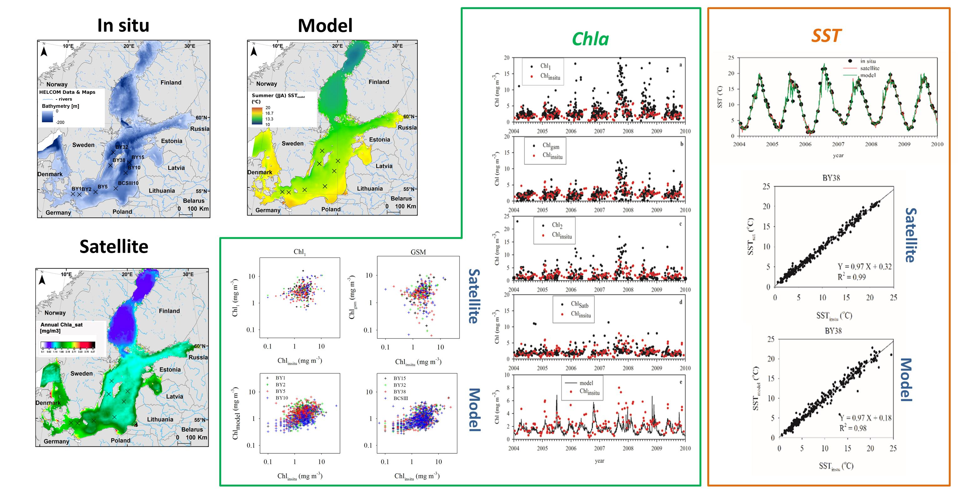
For the evaluation of satellite and model-derived chlorophyll concentration (Chl) and sea surface temperature (SST), we used data from in situ observations. In situ Chl and surface water temperature data were obtained from public databases of the International Council for the Exploration of the Sea (ICES Dataset on Ocean Hydrography, https://ocean.ices.dk, accessed on 1 November 2020). 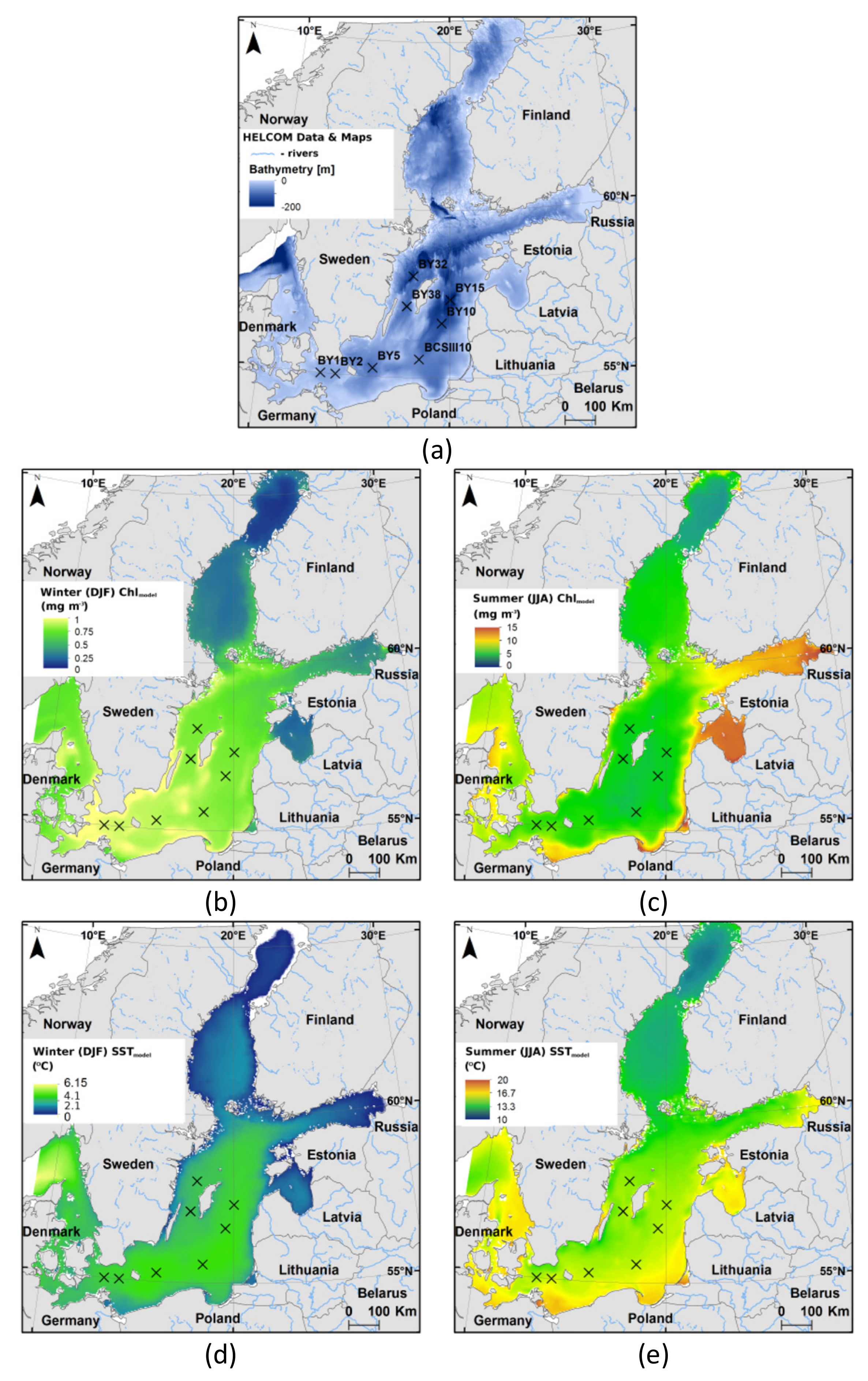Data were collected as part of the HELCOM (The Baltic Marine Environment Protection Commission) program according to their protocols (https://helcom.fi/helcom-at-work/publications/manuals-and-guidelines/, accessed on 1 November 2020). For our analyses, we selected eight stations located in the open sea and representative of the Baltic Proper waters. The geographical positions of these stations are listed in

Table 1. Geographical positions of in situ stations.

Station	Latitude	Longitude
BY1	55.00° N	13.30° E
BY2	55.00° N	14.08° E
BY5	55.25° N	15.98° E
BY10	56.63° N	19.58° E
BY15	57.33° N	20.05° E
BY32	58.02° N	17.98° E
BY38	57.12° N	17.67° E
BCSIII	55.55° N	18.40° E

and shown in Figure 1.

Satellite Chl data used in this paper include four data products (

Table 2. Summary of the satellite sensors and data sets included in GlobColour data products.

	Sensor	SeaWiFS	MERIS	MODIS AQUA	VIIRS NPP	OLCI-A
	Start	4 September 1997	28 April 2002	3 July 2002	2 January 2012	25 April 2016
	End	11 December 2010	8 April 2012	Present	Present	Present
	Reprocessing	NASA R.2018	ESA 3rd	NASA R.2018	NASA R.2018	ESA PB 2.16 to 2.55
Data set
Chl1		X	X	X	X	X
ChlGSM		X	X	X	X	X
Chl2			X			X
ChlSatb				X

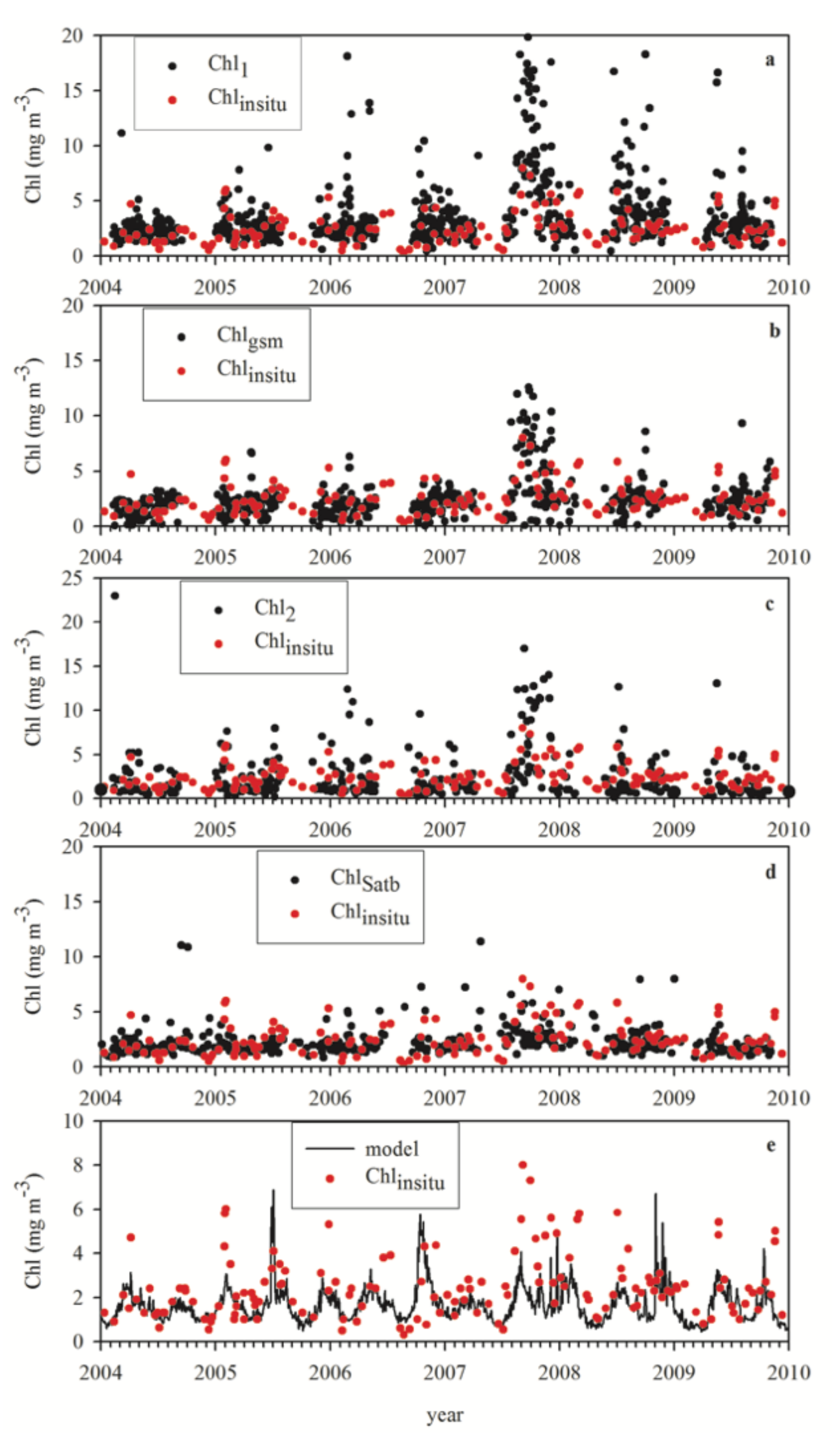
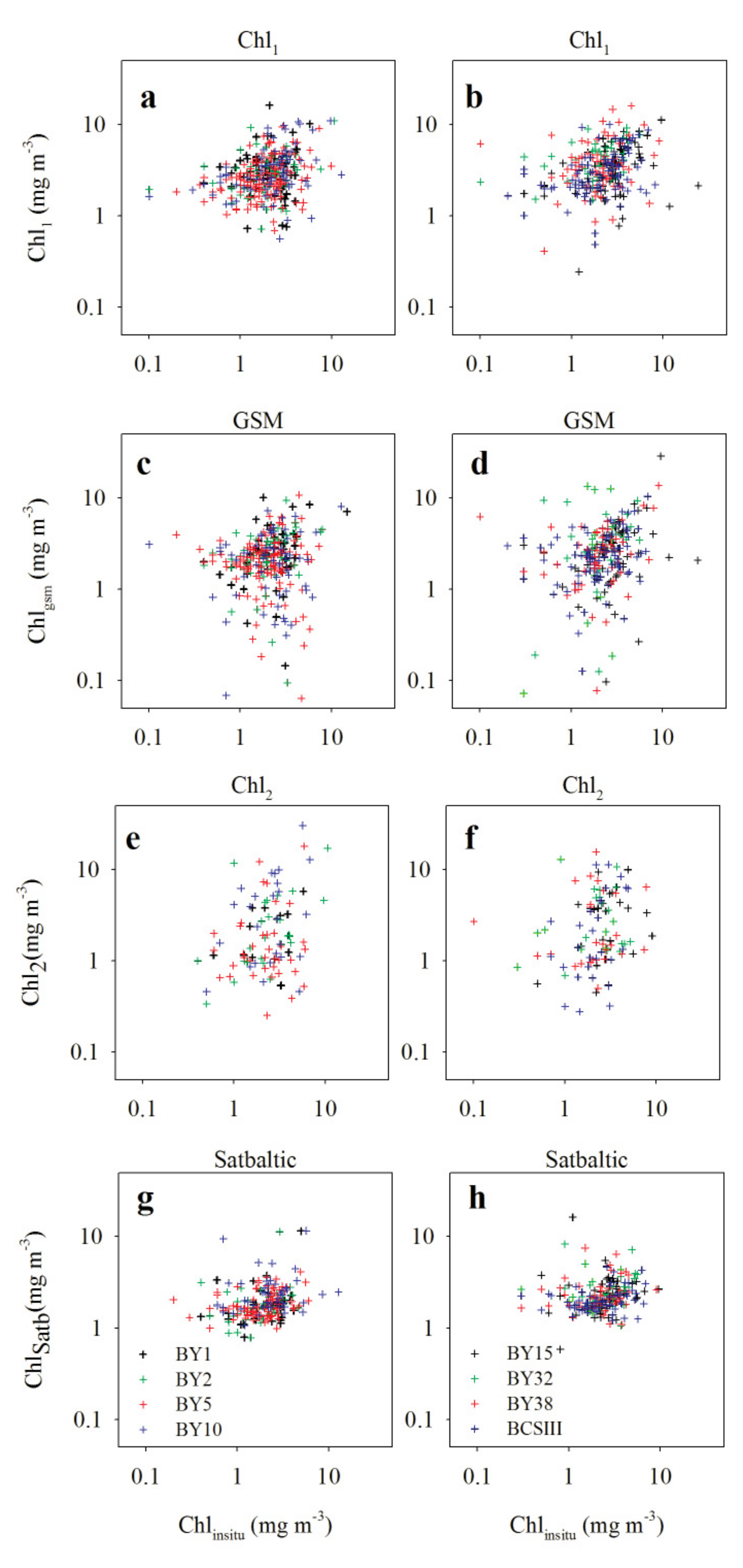
). Three products [34] were downloaded from the GlobColour website on 3 November 2020 (http://globcolour.info, accessed on 1 November 2020). These are: (1) the weighted averaging surface chlorophyll concentration listed in the GlobColor website as CHL1 and in this paper referred to as Chl₁. Estimates of Chl₁ were derived using the reflectance band ratio algorithm [4]; (2) the surface chlorophyll concentration obtained with the GSM algorithm (Chl_gsm) [35,36]; (3) the surface chlorophyll concentration derived from a neural network algorithm [37], in the GlobColour website referred to as Chl2 and in our paper indicated as Chl₂. Finally, the fourth satellite product was the surface Chl concentration estimated with the regional SatBaltic algorithm (Chl_Satb) [38,39]. In the SatBaltic system, the chlorophyll algorithm has been frequently updated (see http://www.satbaltyk.pl, accessed on 1 November 2020). We used data processed with the most recent algorithm at the time of manuscript preparation (version 2020). We did not include Copernicus Marine Environment Monitoring Service’s (CMEMS) data in our analysis, as these data have already been evaluated by several authors, including service providers [40]. Full details of the approach used by GlobColour in the standard processing of satellite ocean color data are provided in the manual (GlobColour Product User Guide GC-UM-ACR-PUG-01 version 4.2.1, March 2020) [41]. Spatial resolution of satellite data is about 1 km.

Both Chl₁ and Chl_gsm data products are surface Chl concentration determinations based on the standard global ocean algorithms [4,35,36] and use, as an input, merged data from several ocean color sensors observing the Earth during a given day, when surface Chl was estimated (Table 2). Time series of these two Chl products began when SeaWiFS started to deliver data in September of 1997. For our work, we used data from years 1998–2019. The SatBaltic data product is based on regionally modified remote sensing reflectance band ratio relationships [38,39]. It was created from the MODIS Aqua observations that started in 2002. The Chl₂ data product was derived using the neural network algorithm established to estimate surface Chl in coastal regions [37]. The Chl₂ data set available at GlobColor was generated only from MERIS and OLCI-A. This is why it includes a significantly smaller number of data points coincident with in situ measurements than in the case of all the other Chl products used in this study.

Table 3. Summary of the error statistics, i.e., the mean absolute error (MAE), bias (B), and the root mean square error (RMSE) for the Chl₁ (mg/m³). N is the number of data pairs used in error calculations. R is correlation coefficient, indicated in bold when correlation was statistically significant (95% confidence level, p < 0.05). Subscript L indicates statistics on log-transformed data.

Station Name	N	Basic Statistics				Statistics for Log-Transformed Data
		MAE	B	RMSE	R	RL	BL	MAEL
BY1	71	1.89	1.23	2.76	0.35	0.20	1.58	2.09
BY2	68	1.40	0.93	1.96	0.36	0.36	1.78	2.09
BY5	157	1.43	0.77	1.89	0.28	0.29	1.55	1.95
BY10	78	1.95	0.95	2.75	0.16	0.28	1.62	2.19
BY15	81	1.85	0.29	3.40	0.08	0.24	1.32	1.95
BY32	51	2.43	2.34	2.96	0.42	0.35	2.63	2.69
BY38	79	2.50	1.93	3.54	0.11	0.26	2.0	2.34
BCSIII	103	1.64	0.91	2.18	0.21	0.35	1.70	2.14
All stations
Full years	688	2.49	1.80	4.55	0.20	0.28	1.70	2.14
Spring	233	2.65	1.28	5.26	0.15	0.23	1.55	2.29
Summer	319	2.78	2.55	4.68	0.29	0.37	1.91	2.04
Fall	110	1.63	0.89	2.66	0.15	0.12	1.17	1.73
Winter	26	1.27	0.99	1.44	0.14	0.05	2.63	3.16

,

Table 4. Summary of the error statistics, i.e., the mean absolute error (MAE), bias, and the root mean square error (RMSE) for the Chl_gsm (mg m⁻³). N is the number of data pairs used in error calculations. R is correlation coefficient, indicated in bold when correlation was statistically significant (95% confidence level, p < 0.05). Subscript L indicates statistics on log-transformed data.

Station Name	N	Basic Statistics				Statistics for Log-Transformed Data
		MAE	B	RMSE	R	RL	BL	MAEL
BY1	48	1.51	0.33	2.26	0.41	0.29	0.93	1.82
BY2	56	1.27	0.44	1.69	0.38	0.38	1.17	1.82
BY5	118	1.41	0.11	1.89	0.08	0.09	1.02	204
BY10	61	1.74	−0.20	2.16	0.31	0.11	0.87	2.34
BY15	61	2.14	−0.33	4.31	0.26	0.24	0.83	1.95
BY32	41	2.39	1.79	3.82	0.17	0.29	1.45	2.57
BY38	58	1.47	0.41	2.01	0.54	0.12	1.00	2.24
BCSIII	79	1.39	0.25	1.80	0.42	0.26	1.10	1.95
All stations
Full years	522	1.61	0.26	2.53	0.30	0.16	1.02	2.09
Spring	159	1.84	−0.76	3.02	0.28	0.13	1.35	2.45
Summer	259	1.54	0.75	2.30	0.52	0.27	1.17	1.82
Fall	82	1.37	0.36	2.31	0.02	0.02	0.93	1.82
Winter	22	1.70	1.56	2.01	0.04	0.0	3.31	3.80

,

Table 5. Summary of the error statistics, i.e., the mean absolute error (MAE), bias, and the root mean square error (RMSE) for the Chl₂ (mg m⁻³). N is the number of data pairs used in error calculations. R is correlation coefficient, indicated in bold when correlation was statistically significant (95% confidence level, p < 0.05). Subscript L indicates statistics on log-transformed data.

Station Name	N	Basic Statistics				Statistics for Log-Transformed Data
		MAE	B	RMSE	R	RL	BL	MAEL
BY1	13	1.08	−0.28	1.46	0.49	0.30	0.83	1.74
BY2	25	1.97	0.21	3.04	0.58	0.56	0.89	1.91
BY5	37	2.30	−0.19	3.51	0.21	0.08	0.66	2.51
BY10	26	3.74	2.04	5.97	0.42	0.31	1.12	2.63
BY15	25	2.33	0.06	2.99	0.10	0.29	0.85	2.14
BY32	23	2.52	1.05	3.59	0.05	0.17	1.26	2.29
BY38	26	2.67	0.77	3.86	0.05	0.07	1.10	2.69
BCSIII	28	2.03	0.70	2.93	0.44	0.40	0.85	2.29
All stations
Full years	203	2.40	0.56	3.71	0.28	0.26	0.91	2.29
Spring	78	2.82	0.01	3.90	0.29	0.23	0.81	2.63
Summer	86	2.59	1.42	4.29	0.30	0.32	1.15	2.14
Fall	39	1.36	−0.25	1.86	0.35	0.29	0.71	1.91
Winter	0	-	-	-	-	-	-	-

and

Table 6. Summary of the error statistics, i.e., the mean absolute error (MAE), bias, and the root mean square error (RMSE) for the Chl_Satb (mg m⁻³). N is the number of data pairs used in error calculations. R is correlation coefficient, indicated in bold when correlation was statistically significant (95% confidence level, p < 0.05). Subscript L indicates statistics on log-transformed data.

Station Name	N	Basic Statistics				Statistics for Log-Transformed Data
		MAE	B	RMSE	R	RL	BL	MAEL
BY1	39	1.09	−0.23	1.57	0.41	0.27	0.89	1.62
BY2	38	0.92	0.13	0.98	0.24	0.27	1.07	1.55
BY5	92	0.79	−0.17	1.07	0.35	0.33	1.05	1.62
BY10	47	1.61	−0.01	2.67	0.12	0.16	1.10	1.78
BY15	53	1.47	−0.23	2.71	0.07	0.10	0.91	1.66
BY32	45	1.11	0.06	1.68	0.21	0.01	1.18	1.70
BY38	54	1.15	−0.03	1.72	0.14	0.16	1.07	1.62
BCSIII	63	1.12	−0.50	1.55	0.33	0.25	0.93	1.62
All stations
Full years	431	1.13	−0.15	1.85	0.18	0.14	1.02	1.66
Spring	109	1.52	−0.07	2.51	0.04	0.10	1.15	2.04
Summer	242	0.91	−0.38	1.43	0.43	0.51	0.91	1.45
Fall	62	1.05	0.01	1.58	0.12	0.13	0.98	1.51
Winter	18	1.84	1.70	264	0.03	0.10	2.63	2.75

list the exact numbers of coincident satellite/in situ data pairs available at each station for each Chl product. In these comparisons, we used data from pixels containing coincident in situ data points from in situ stations. Only data pairs with in-situ measurements and satellite determinations for the same day were used in comparisons. This match-up criterium allowed us to build a data set with a sufficiently large number of observations, but is not as strict as that used in [8] for algorithm development and validation. We feel that our approach is justified, since in most situations in the open Baltic Sea we do not expect large changes in Chl concentrations over the course of a day. In addition, we do not propose to establish new remote sensing relationships, but only assess different satellite data sets. Our goal was to show the potential users of these data what differences between in situ and remote sensing data can be expected.

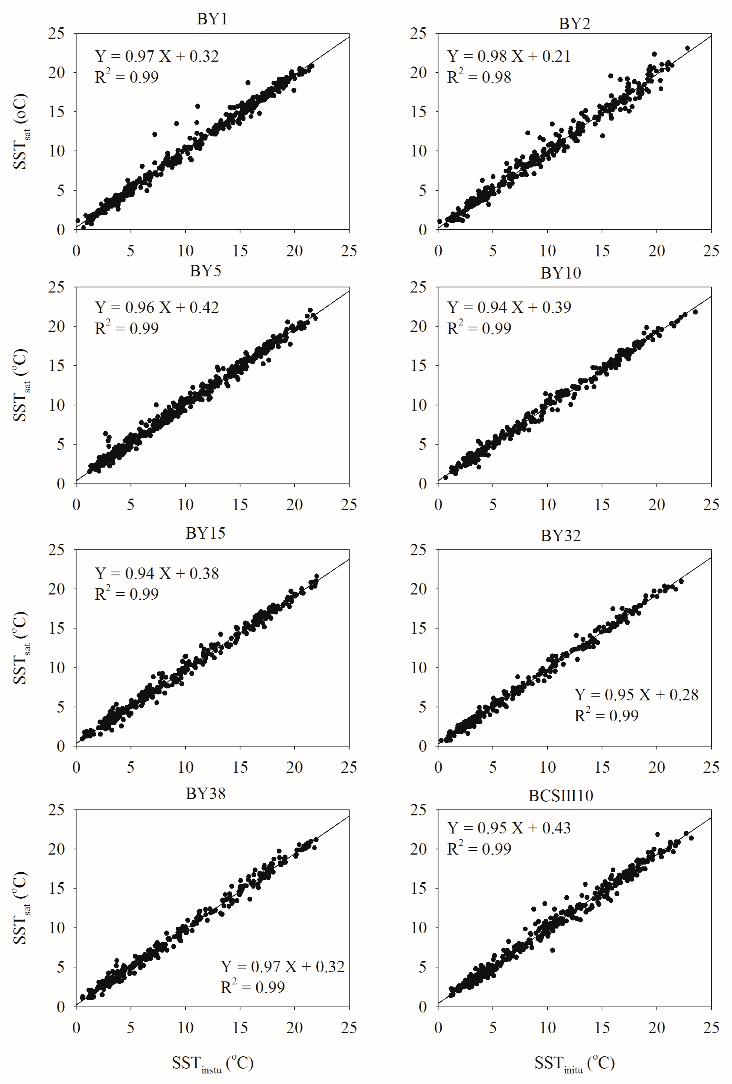
There are several satellite SST data products available as open-access data for the Baltic Sea. We decided to use a data series known as the National Oceanic and Atmospheric Administration (NOAA) daily Optimum Interpolation SST Version 2 data set (dOISST.v2). The dOISST.v2 data set is available at the National Centers for Environmental Information (NCEI) website, under the name “NOAA Optimum Interpolation 1/4 Degree Daily Sea Surface Temperature (OISST) Analysis, Version 2” (with doi:10.7289/V5SQ8XB5). The same data are distributed elsewhere, for example, at the Physical Oceanography Distributed Active Archive Center (PODAAC) of the Jet Propulsion Laboratory, NASA, as the GHRSST (Group for High Resolution SST) Level 4 AVHRR_OI Global Blended Sea Surface Temperature Analysis (with doi:10.5067/GHAAO-4BC01). The dOISST.v2 data set has been approved by the NOAA Climate Data Record (CDR) program as an operational CDR. It meets the definition of CDR put forward by the National Research Council (2004), as it is of sufficient length, consistency, and continuity to determine climate variability. These global daily SST records (one daily value for each pixel), with spatial resolution of 0.25° by 0.25°, are based on the Advanced Very High Resolution Radiometer (AVHRR) infrared satellite measurements (Pathfinder from September 1981 through December 2005, operational AVHRR from January 2006). The final global data set was derived combining satellite SST retrievals with SST observations from ships and buoys, and proxy SSTs generated from sea ice concentrations. The full description of data processing methods and comparisons between the NOAA dOISST.v2 and in situ data can be found in [42,43]. Note that the infrared satellite remote sensing SST algorithms can provide either a skin SST, if they are based on radiative transfer models, or a subskin SST, if in situ observations have been used to adjust satellite retrievals. In the dOISST.v2 data set, the bias correction of the satellite data is based on data from ships and buoys, and therefore it should be interpreted as the bulk SST [7]. In order to apply the correction for bias, the satellite data were classified into daytime and nighttime bins and corrected separately using in situ data. Then, all the data were reanalyzed jointly using the optimum interpolation (OI) procedure. The final data represent the daily mean bulk SST values representative for the top 1 m surface water layer.

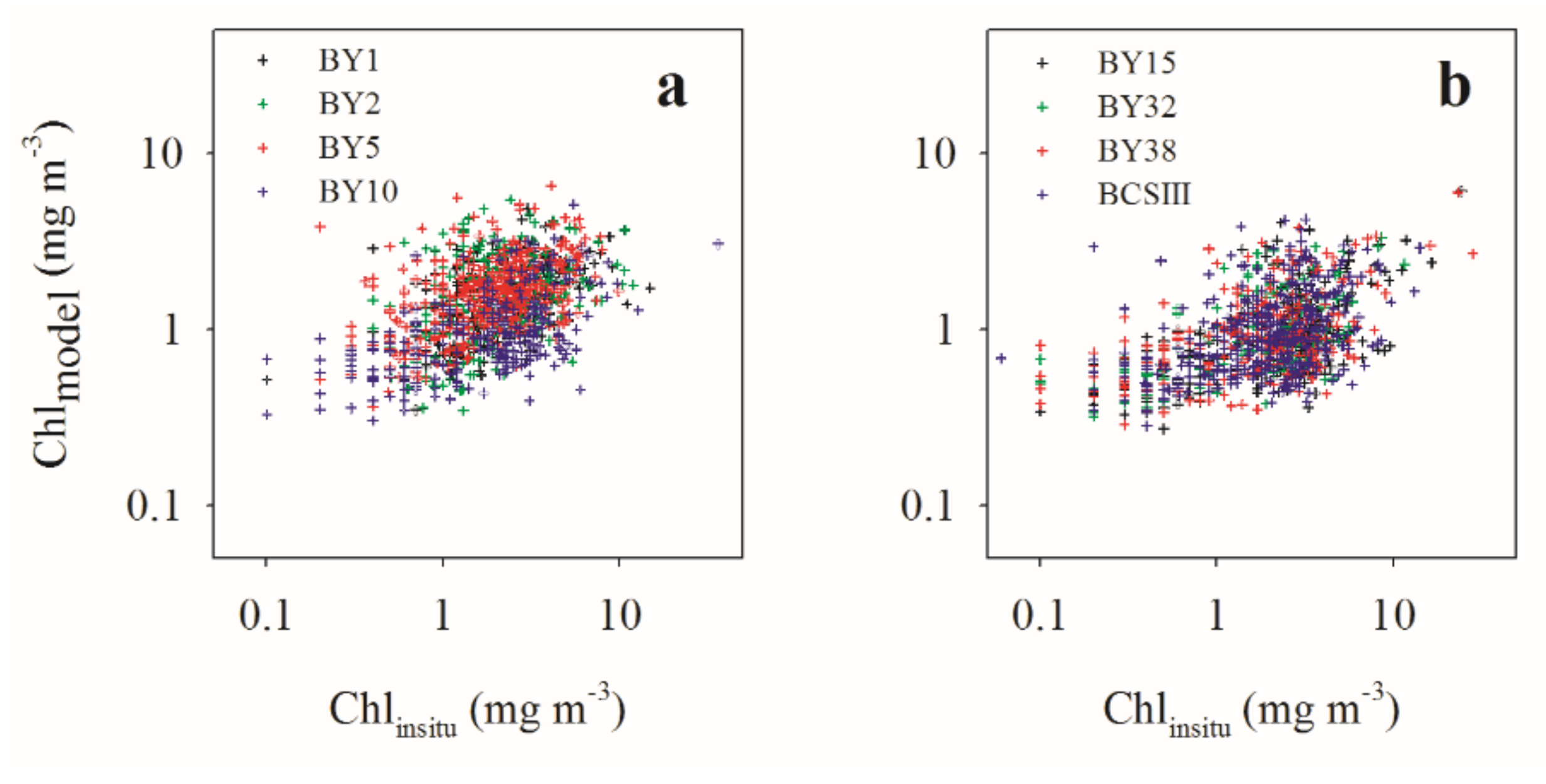
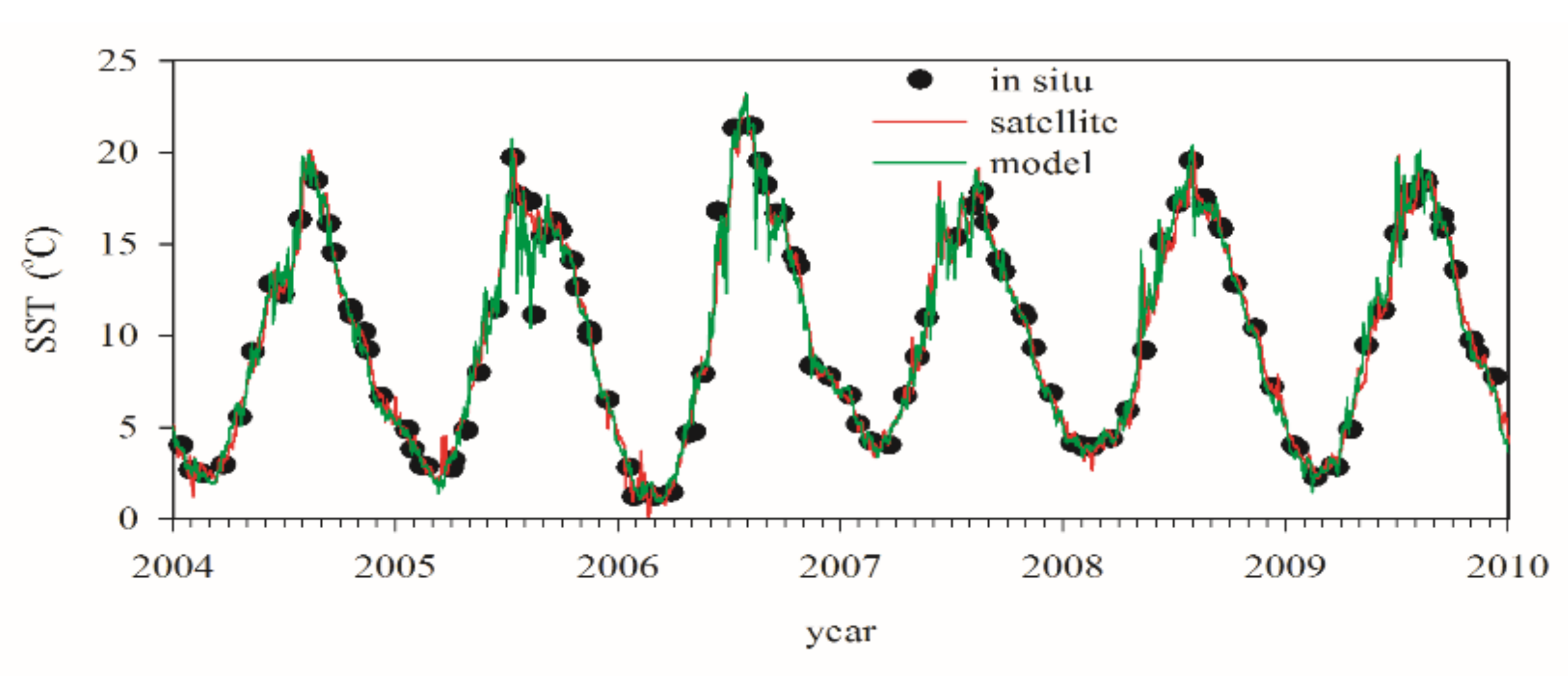
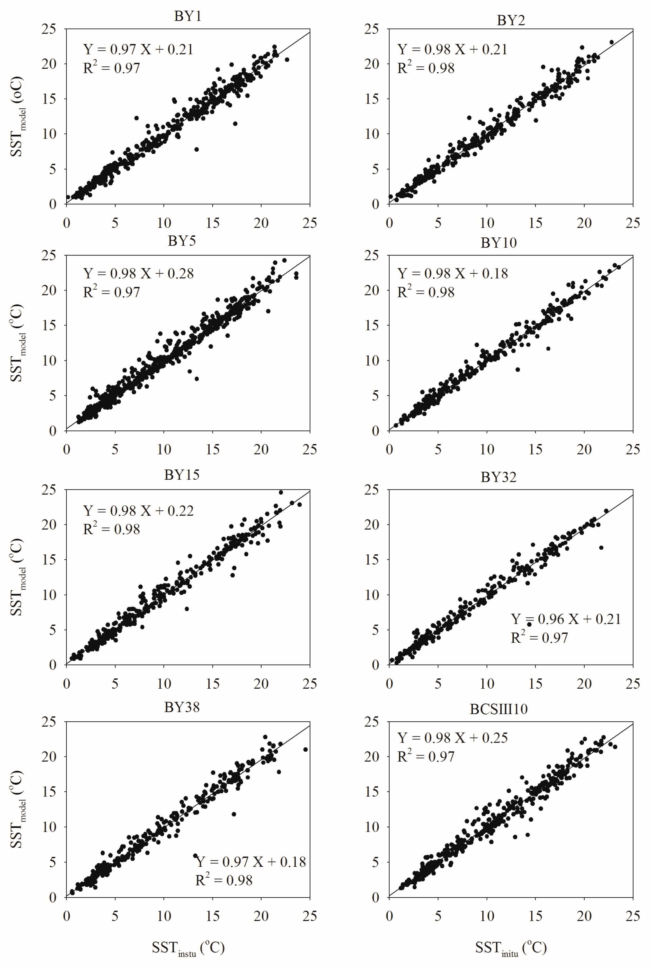
The modeled SST and surface Chl data (indicated as SST_model and Chl_model) used in our comparisons were extracted from the Baltic Sea biogeochemical reanalysis data set (BALTICSEA_REANALYSIS_BIO_003_012) provided by the Copernicus Marine Environment Monitoring Service’s (CMEMS) Baltic Monitoring and Forecasting Centre (BAL MFC). These reanalysis data were derived using the ice-ocean NEMO (Nucleus for European Modelling of the Ocean) model [44]. NEMO was coupled with the biogeochemical model SCOBI (Swedish Coastal and Ocean Biogeochemical model). The horizontal grid resolution is approximately 2 nautical miles (latitude 0.03333 degrees; longitude 0.05556 degrees), and there are 56 water depth levels. The reanalysis applied the Localized Singular Evolutive Interpolated Kalman (LSEIK) filter for data assimilation [45]. The observational data used for data assimilation included SST, nitrate, phosphate, ammonium, and dissolved oxygen concentrations. For comparison with satellite and in situ data, we selected data from 1998–2019 at grid points located at the shortest possible distance from the in situ stations and from the same day as the in situ observations. Data originated from the uppermost available model depth level (~1.5 m). More details on the model setup can be found in the PRODUCT USER MANUAL Baltic Sea Biogeochemical Reanalysis Product (BALTIC SEA_REANALYSIS_BIO_003_012, CMEMS-BAL-PUM-003-012 version 2) [46].

Table 7. Summary of the error statistics, i.e., the mean absolute error (MAE), bias, and the root mean square error (RMSE) for the Chl (mg m⁻³) from model. N is the number of data pairs used in error calculations. R is correlation coefficient, indicated in bold when correlation was statistically significant (95% confidence level, p < 0.05). Subscript L indicates statistics on log-transformed data.

Station Name	N	Basic Statistics				Statistics for Log-Transformed Data
		MAE	B	RMSE	R	RL	BL	MAEL
BY1	293	1.21	−0.85	1.77	0.32	0.44	0.71	1.70
BY2	273	1.30	−0.78	1.95	0.24	0.40	0.76	1.91
BY5	465	0.76	−0.54	1.38	0.41	0.44	0.85	1.66
BY10	242	1.55	−1.40	2.97	0.42	0.54	0.56	2.29
BY15	267	1.80	−1.69	2.75	0.59	0.55	0.49	2.51
BY32	160	1.38	−1.21	1.95	0.50	0.52	0.60	2.40
BY38	254	1.56	−1.39	2.84	0.55	0.54	0.56	2.34
BCSIII	357	1.54	−1.38	2.22	0.34	0.40	0.51	2.40
All stations
Full years	2311	0.15	−1.10	2.23	0.36	0.45	0.63	2.09
Spring	575	1.88	−1.26	3.40	0.33	0.48	0.81	2.04
Summer	670	1.57	−1.39	2.05	0.01	0.14	0.48	2.40
Fall	582	1.38	−1.27	1.76	0.08	0.10	0.52	2.04
Winter	484	0.48	−0.3	0.70	0.51	0.50	0.89	1.78

lists the number of coincident model/in situ data pairs available at each station for Chl, while

Table 8. Summary of the error statistics, i.e., the mean absolute error (MAE), bias (B), root mean square error (RMSE), and correlation coefficient (R) between the SST data from in situ measurements and the satellite-based National Oceanic and Atmospheric Administration (NOAA) daily Optimum Interpolation SST Version 2 data set (dOISST.v2). N is the number of data pairs used in calculations. All correlations are statistically significant (95% confidence level, p < 0.05).

Station	N	MAE	Bias	RMSE	R
BY1	442	0.45	0.00	0.69	0.993
BY2	330	0.44	−0.05	0.58	0.995
BY5	545	0.43	0.05	0.59	0.995
BY10	304	0.51	−0.19	0.66	0.996
BY15	347	0.47	0.03	0.62	0.995
BY32	246	0.49	−0.18	0.62	0.996
BY38	314	0.48	−0.12	0.61	0.996
BCSIII	419	0.55	−0.12	0.75	0.993
All stations
Full years	2947	0.48	−0.09	0.65	0.995
Spring	758	0.45	−0.20	0.63	0.975
Summer	912	0.62	−0.32	0.78	0.976
Fall	683	0.45	−0.21	0.61	0.984
Winter	594	0.38	0.01	0.52	0.954

and

Table 9. Summary of the error statistics, i.e., the mean absolute error (MAE), bias (B), root mean square error (RMSE), and correlation coefficient (R) between the SST data from in situ measurements and reanalysis model. N is the number of data pairs used in calculations. All correlations are statistically significant (95% confidence level, p < 0.05).

Station	N	MAE	Bias	RMSE	R
BY1	442	0.63	−0.05	0.94	0.987
BY2	330	0.58	0.02	0.84	0.990
BY5	545	0.65	0.12	0.96	0.986
BY10	304	0.53	0.04	0.81	0.991
BY15	347	0.60	0.06	0.91	0.988
BY32	246	0.60	−0.12	0.98	0.987
BY38	314	0.61	−0.08	0.96	0.976
BCSIII	419	0.65	0.04	0.99	0.986
All stations
Full years	2947	0.61	0.01	0.93	0.987
Spring	758	0.59	0.44	0.85	0.974
Summer	912	0.85	0.08	1.18	0.934
Fall	683	0.51	−0.32	0.69	0.982
Winter	594	0.33	−0.19	0.49	0.966

list the number of data pairs available for satellite/in situ and model/in situ SST comparisons, respectively.

3.2. Methods

The differences between in situ and satellite (or model) derived data were quantified by standard statistical methods. First, comparisons between the data sets in linear space included the root mean square error (RMSE), the bias (B), the mean absolute error (MAE), and the Pearson’s correlation coefficient (R) for all types of data pairs. The bias (B) was defined as the mean difference between the estimated data value (from model or satellite algorithms) and the in situ measurement:

$$\mathrm{B}=\frac{1}{\mathrm{N}} {\displaystyle \sum }_{\mathrm{n}=1}^{\mathrm{N}}{\mathrm{P}}_{\mathrm{n}}-\frac{1}{\mathrm{N}} {\displaystyle \sum }_{\mathrm{n}=1}^{\mathrm{N}}{\mathrm{O}}_{\mathrm{n}}$$

(1)

where N is the total number of measurements, O_n is the value measured in situ, and P_n is the predicted value (satellite or model, Chl or SST determination). The root mean square error (RMSE) was calculated as:

$$\mathrm{RMSE}={\left[\frac{1}{\mathrm{N}-1}{\displaystyle \sum }_{\mathrm{n}=1}^{\mathrm{N}}{\left({\mathrm{P}}_{\mathrm{n}}-{\mathrm{O}}_{\mathrm{n}}\right)}^2\right]}^{\raisebox{1ex}{$1$}\!\left/ \!\raisebox{-1ex}{$2$}\right.}$$

(2)

The mean absolute error (MAE) was calculated using the following formula:

$$\mathrm{MAE}=\frac{1}{\mathrm{N}}{\displaystyle \sum }_{\mathrm{n}=1}^{\mathrm{N}}\left|{\mathrm{P}}_{\mathrm{n}}-{\mathrm{O}}_{\mathrm{n}}\right|$$

(3)

Additionally, Chl data were log-transformed. In this case in the formulas listed above

$${\mathrm{O}}_{\mathrm{n}}={\log }_{10}\left({\mathrm{Chl}}_{\mathrm{insitu}}\right)$$

(4a)

$${\mathrm{P}}_{\mathrm{n}}={\log }_{10}\left({\mathrm{Chl}}_{\mathrm{satellite}}\right) \mathrm{or} {\mathrm{P}}_{\mathrm{n}}={\log }_{10}\left({\mathrm{Chl}}_{\mathrm{model}}\right)$$

(4b)

Following [47], for Chl log-transformed data, the bias (B_L), the mean absolute error (MAE_L), and the Pearson’s correlation coefficient were calculated. Ocean color Chl determinations are usually log-transformed prior to calculation of error metrics, because the data values frequently span multiple orders of magnitude [47]. This log-transformation results in a conversion of the statistical metrics from linear to multiplicative space. In general, the choice of either linear or multiplicative metrics depends on the properties of the variable of interest. For example, water temperature is always evaluated with linear metrics. Data such as Chl, spanning multiple orders of magnitude and with the uncertainty that varies proportionally with the data value, are better assessed using multiplicative metrics [48]. The bias (B_L) and the mean absolute error (MAE_L) listed in the Tables were calculated as:

$${\mathrm{V}}_{\mathrm{conv}}={10}^{\mathrm{Vlog}}$$

(5)

where V_conv is either B_L or MAE_L converted out of the log-space and V_log is its value calculated on log-transformed data. After this back transformation, the errors can be interpreted as a percentage. For example, a B_L of 1.5 indicates that the estimated value is on average 1.5× (50%) greater than the observed data, while a MAE_L of 1.6 indicates an average relative error of 60%.

When comparing the in situ and satellite-derived data, one has to remember that both kinds of data are subject to errors. For example, in situ data include errors due to the limited precision of instrumentation used in the experiments. It is logical to expect that errors in satellite and model data can be larger than in in situ measurements. These errors are due to the assumptions used to calculate the values and approximate nature of algorithms. However, even if all data used in this paper are expected to be subject to errors, we refer to in-situ data as ‘measured’ and to the differences between satellite or model derived and in-situ estimates as ‘errors’. Regressions listed in this paper represent Model II major-axis reduced regression [49], as this type of regression model is suitable when the two variables in the regression equation contain errors.

4. Results

Our comparisons are based on data collected at stations located in the western to central parts of the Baltic Sea (Figure 1a). Multiyear mean SST_model and surface Chl_model (calculated from model reanalysis) for the winter and summer seasons for the entire Baltic Sea are displayed in Figure 1b–e. As can be seen, the northern and eastern Baltic Sea (Gulfs of Bothnia, Finland, and Riga) were characterized by different mean SST and surface Chl values than the regions discussed in this paper. Waters in these regions may have somewhat different optical properties than in the central parts of the Baltic Sea, but there are no sufficient long-term in situ data to extend our analyses to these regions.

4.1. Chl Comparisons

In Figure 2a–e, example Chl time series used in our analysis are displayed. For brevity, we only displayed data as recorded in years 2004–2009 at station BY5. Each panel includes a set of data points derived by a different satellite algorithm or by the numerical model and compares them with in situ measurements shown as red dots. In Figure 2e, we can clearly see an annual cycle in modeled Chl. We note that, generally, satellite data (Chl₁, Chl_gsm, Chl₂, and Chl_Satb) are missing in the late fall to early spring time interval (when low Chl values were observed in situ). This is due to the persistent overcast sky conditions over the Baltic Sea during this time of the year [18]. Data in Figure 2a–d show that often satellite estimates were higher than the highest in situ measurements in the same year. In addition, satellite data were characterized by large scatter of data points. According to Figure 2e, the modeled Chl did not always agree with in situ measurements as well, in particular when in situ vales were high.

To better visualize the relationships between different data sets, we plotted, in Figure 3a–h, scatterplots for different satellite estimates of Chl (Chl₁, Chl_gsm, Chl₂, and Chl_Satb) as a function of in situ Chl determinations. Diverse symbols were used to indicate different stations in order to verify if there was any significant difference between the stations. Error statistics and correlation coefficients are listed in Table 3, Table 4, Table 5 and Table 6. Similarly, the comparison of modeled and in situ Chl data is displayed in Figure 4, and the errors statistics are listed in Table 7. Generally, the results did not support the notion that there is a clear dependence of the relationships on the geographical position of the station; therefore, it seems that in the open Baltic Sea large scale circulation patterns and distribution of water masses do not significantly influence algorithm performance. Tables also show statistics for full data sets (all stations combined together). Error estimates were large in all satellite estimates (Table 3, Table 4, Table 5 and Table 6). The smallest bias in satellite data was estimated for Chl₂. The SatBaltic estimates had the lowest values of RMSE and MAE (liner and logarithmic estimates), but Chl₁ estimates seemed to be better correlated with in situ observations (low, but statistically significant correlation coefficient R at most stations and for the entire data set when data from all stations are merged). As can be seen in Table 7, there was a statistically significant correlation between in situ and modeled Chl in all cases (at all stations and in full data set). The model, on average, underestimated the in situ Chl concentrations.

The tables compare statistics for full data sets (all stations combined together) and data divided into the seasons of the year. The seasons were defined in the following way. Winter includes data from December to February, spring includes March to May, summer includes June to August, and fall consists of September to November. We can see that the performance of ocean color satellite algorithms depends on the season of the year. All algorithms performed best during summer. In particular, high R and low bias and errors are shown in the results for the SatBaltic algorithm during summer. This seasonal variability in the algorithm performance can be related to the fact that bulk optical properties of seawater change during the course of the year in response to variable concentrations of optically significant water components (e.g., Chl, suspended, and dissolved organic matter concentrations). In addition, specific optical properties (per unit of mass) of different components can also vary depending on the season. For example, it is well known that bulk optical properties of phytoplankton depend on the main species present in the water. Therefore, the specific absorption and scattering properties of phytoplankton are clearly different during spring bloom composed mainly of diatoms or cyanobacteria blooms during summer [50,51]. One of the reasons why the SatBaltic regional ocean color algorithm performs so well during summer can be that most of the data used to derive this algorithm were collected during summers. This is because at this time of the year it is more probable to encounter sunny days with clear skies in this region and therein collect simultaneous in situ and satellite data.

In addition, atmospheric corrections are more likely to have larger errors when the sun is at low angles and sea surface is covered by whitecaps due to the stormy weather encountered often in late fall, winter, and early spring. According to our results, it may be worthwhile to try, in the future, to derive seasonal versions of the ocean color algorithms for the Baltic Sea and to verify if such an approach could improve the overall performance of ocean color remote sensing in this region. If we look at the seasonal performance of the numerical model simulations of Chl (Table 7), we can see that the model simulations showed low correlations with in situ data collected in summer and fall. This means that the model was able to simulate seasonal cycles, but did not reproduce well the interannual variability in the Chl concentration in the summer and fall seasons.

4.2. Sea Surface Temperature Comparisons

Figure 5 presents an example time series of in situ, satellite, and modeled determinations of sea-surface temperature. We can see that, in contrast to the Chl time series shown in Figure 2, there is a good agreement between different estimates of SST. Figure 6 and Figure 7 show scatter plots for SST determinations. There were statistically significant linear relationships between SST_sat and SST_insitu (Figure 6) as well as between SST_model and SST_insitu (Figure 7) at all stations. R² coefficients were somewhat higher in the case of SST_sat relationship with in situ data. Table 8 and Table 9 summarize the error statistics for the data sets presented in Figure 6 and Figure 7. At the bottom of these Tables, the error estimates for the full data sets with all stations combined together are shown. Apart from these, the data sets were divided into seasons in the same way as it was done for the Chl estimates. The results showed, again, that the correlation of modeled and satellite SST estimates with in situ data was always high. Somewhat surprisingly, the model SST during summer showed a little lower correlation and larger RMSE than all the other SST estimates, but the bias was low. Summarizing, the results for SST comparisons indicated that the performance of satellite and model SST determinations was acceptable at all stations investigated. Recall that, in contrast, our results shown in the previous section clearly underlined the fact that more efforts are needed to develop more reliable satellite Chl algorithms and numerical phytoplankton models for the Baltic Sea.

5. Conclusions

Our goal in this paper was to assess available open-access data sets, often used to characterize the environmental status of the Baltic Sea. Two important environmental variables were considered, SST and Chl. Our results confirmed that satellite and model estimates of SST in the Baltic Sea are reliable and agree with in situ data. Unfortunately, this is not the case with satellite and model predictions of surface Chl concentrations. We evaluated four satellite-based surface Chl concentration data sets. It has to be stressed that, even if our analysis used data collected over a long time interval and was based on all available match-up data pairs for evaluated types of data products at several geographical positions, the number of coincident in situ and satellite Chl determinations was much smaller than in the case of the modeled Chl. This is due to the fact that, in the Baltic Sea, the sky is often covered by clouds. Thus, the evaluation of satellite Chl data products at one geographical position (station) is based on a limited amount of data.

Our results did not suggest that there was a significant difference in the performance of ocean color algorithms between the stations located in the open Baltic Proper. When all data of a given type from all stations were merged, the number of data points was larger, but statistical analysis still showed low correlations between in situ and satellite Chl determinations. In addition, we verified if the performance of satellite algorithms varies with the season of the year. All the satellite Chl data products showed better agreement with in situ data during summer. There may be several reasons for this. During summer there are more days with clear skies and this results in larger data sets with matchups. In addition, the range of observed Chl values was larger in the spring/summer time interval. On the other hand, even if there are clear skies in winter or fall, the atmospheric correction may not work as well when the sun is at low angles and the sea is stormy and covered with whitecaps. In seasonal data, the best correlation, low bias and errors were observed for Chl_Satb satellite data product in summer. If the entire data sets with various Chl data products were considered (all years and stations combined), the best correlation and the largest number of matchups was for the Chl₁ data product. This relatively large number of data points was due to the fact that this data product is based on several available ocean color data sets obtained from different satellite missions combined together, and covers the longest time interval. However, even if the correlation was statistically significant, Chl₁ represents large errors in comparison with in situ data. The smallest bias from all satellite data products covering full calendar years (all seasons) was determined for Chl₂, but the correlation with in situ data was low. In comparison with satellite data, model reanalysis delivered Chl determinations that were well correlated with in situ data, but still there were significant differences between measured and predicted Chl values. In particular, it seems that the model did not simulate well a full range of variability of measured Chl values. In addition, when multiyear seasonal data were considered, we observed that model results were less reliable during summer than in other seasons. It seems that the model was not able to precisely simulate dynamic changes taking place during summer cyanobacteria blooms. This has to be kept in mind when using these data to evaluate the ecological changes in the Baltic Sea. Summarizing, it seems that if long-term Chl predictions have to be used in research, Chl determinations from model reanalysis (after some corrections) present a better perspective than the satellite data. Satellite data are more reliable during summer than in other seasons. It is our belief that a large and variable inflow of river waters with high concentrations of colored organic matter and mineral sediments, as well as irregular inflows of oceanic water with completely different optical properties, make the Baltic Sea one of the most complex and difficult regions to apply optical remote sensing methods. Hopefully, with more effort, it will be possible in the near future to assemble larger and more complete data sets with diverse types of optical data to develop more advanced regional ocean color algorithms designed specifically for the Baltic Sea. Perhaps one of the first developments will be to account for seasonal variability. Another prospect for the future may be to devise a strategy to derive a new Chl product for the Baltic Sea that could use a combination of model/satellite data as an input. Such product would take advantage of the fact that during summer, satellite data allow for better tracing of massive blooms developing at this time of the year, while models are more reliable at these times when the weather severely limits optical remote sensing. In our final word, we would like to stress that even if scientists continue to strive to decrease errors and improve satellite methods in coastal seas, the substantial scientific benefits from the use of large-scale ocean color satellite observations for the global oceanography are unquestionable.

References

1. Axell, L.; Huess, V.; Derval, C. PUM for the Baltic Sea Biogeochemical Reanalysis Product, E.U. Copernicus Marine Service Information. 2019. Available online: http://marine.copernicus.eu/documents/PUM/CMEMS-BAL-PUM-003-012.pdf (accessed on 1 November 2020).
2. Morel, A. Optical modeling of the upper ocean in relation to its biogenous matter content (case I waters). J. Geophys. Res. 1988, 93, 749–768. [Google Scholar] [CrossRef] [Green Version]
3. Garver, S.A.; Siegel, D.A. Inherent optical property inversion of ocean color spectra and its biogeochemical interpretation: 1. Time series from the Sargasso Sea. J. Geophys. Res. 1997, 102, 18607–18625. [Google Scholar] [CrossRef]
4. O’Reilly, J.E.; Maritorena, S.; Siegel, D.A.; O’Brien, M.C.; Toole, D.; Mitchell, B.G.; Kahru, M.; Chavez, F.P.; Strutton, P.; Cota, G.F.; et al. Ocean color chlorophyll a algorithms for SeaWiFS, OC2, and OC4: Version 4. SeaWiFS Postlaunch Calibration Valid. Anal. Part 2000, 3, 9–23. [Google Scholar]
5. Merchant, C.J.; LeBorgne, P. Retrieval of sea surface temperature from space, based on modeling of infrared radiative transfer: Capabilities and limitations. J. Atmos. Ocean. Technol. 2004, 21, 1734–1746. [Google Scholar] [CrossRef] [Green Version]
6. Good, S.A.; Corlett, G.K.; Remedios, J.J.; Noyes, E.J.; Llewellyn-Jones, D.T. The global trend in Sea Surface Temperature from 20 years of advanced very high resolution radiometer data. J. Clim. 2007, 20, 1255–1264. [Google Scholar] [CrossRef] [Green Version]
7. Reynolds, R.W.; Smith, T.M.; Liu, C.; Chelton, D.B.; Casey, K.S.; Schlax, M.G. Daily high-resolution-blended analyses for sea surface temperature. J. Clim. 2007, 20, 5473–5496. [Google Scholar] [CrossRef]
8. Bailey, S.W.; Werdell, P.J. A multi-sensor approach for the on-orbit validation of ocean color satellite data products. Remote Sens. Environ. 2006, 102, 12–23. [Google Scholar] [CrossRef]
9. Mobley, C.D. Light and Water. Radiative Transfer in Natural Waters; Academic Press: San Diego, CA, USA, 1994. [Google Scholar]
10. Darecki, M.; Stramski, D. An evaluation of MODIS and SeaWiFS bio-optical algorithms in the Baltic Sea. Remote Sens. Environ. 2004, 89, 326–350. [Google Scholar] [CrossRef]
11. Behringer, D.W.; Xue, Y. Evaluation of the global ocean data assimilation system at NCEP: The Pacific Ocean. In Proceedings of the Eighth Symposium on Integrated Observing and Assimilation Systems for Atmosphere, Oceans, and Land Surface, AMS 84th Annual Meeting, Washington State Convention and Trade Center, Seattle, Washington, DC, USA, 11–15 January 2004. [Google Scholar]
12. Derber, J.C.; Rosati, A. A global oceanic data assimilation system. J. Phys. Oceanogr. 1989, 19, 1333–1347. [Google Scholar] [CrossRef] [Green Version]
13. Penny, S.G.; Behringer, W.D.; Carton, J.A.; Kalnay, E. A hybrid global ocean data assimilation system at NCEP. Mon. Wea. Rev. 2015, 143, 4660–4677. [Google Scholar] [CrossRef]
14. Storto, A.; Alvera-Azcárate, A.; Balmaseda, M.A.; Barth, A.; Chevallier, M.; Counillon, F.; Domingues, C.M.; Drevillon, M.; Drillet, Y.; Forget, G.; et al. Ocean Reanalyses: Recent Advances and Unsolved Challenges. Front. Mar. Sci. 2019, 6, 418. [Google Scholar] [CrossRef] [Green Version]
15. Axell, L.; Liu, Y. Application of 3-D ensemble variational data assimilation to a Baltic Sea reanalysis 1989–2013. Tellus A Dyn. Meteorol. Oceanogr. 2016, 68, 24220. [Google Scholar] [CrossRef] [Green Version]
16. Hinrichs, I.; Jahnke-Bornemann, A.; Andersson, A.; Ganske, A.; Gouretski, V.; Jensen, C.; Klein, B.; Möller, J.; Sadikni, R.; Tinz, B. The Baltic and North Seas Climatology (BNSC)-A Comprehensive, Observation-Based Data Product of Atmospheric and Hydrographic Parameters. Front. Earth Sci. 2019, 7, 158. [Google Scholar] [CrossRef]
17. HELCOM. Eutrophication in the Baltic Sea—An integrated thematic assessment of the effects of nutrient enrichment and eutrophication in the Baltic Sea region. In Baltic Sea Environment Proceedings; Helsinki Commission: Helsinki, Finland, 2009; Volume 115B, p. 148. [Google Scholar]
18. Leppäranta, M.; Myrberg, K. Physical Oceanography of the Baltic Sea. Springer-Praxis Book Series in Geophysical Sciences; Springer: Chichester, UK, 2009. [Google Scholar]
19. Matthäus, W.W.; Franck, H. Characteristics of major Baltic inflows-A statistical analysis. Cont. Shelf Res. 1992, 12, 1375–1400. [Google Scholar] [CrossRef]
20. Mohrholz, V.; Naumann, M.; Nausch, G.; Krüger, S.; Gräwe, U. Fresh oxygen for the Baltic Sea-An exceptional saline inflow after a decade of stagnation. J. Mar. Syst. 2015, 148, 152–166. [Google Scholar] [CrossRef] [Green Version]
21. Stramska, M.; Aniskiewicz, P. Satellite Remote Sensing Signatures of the Major Baltic Inflows. Remote Sens. 2019, 11, 954. [Google Scholar] [CrossRef] [Green Version]
22. Neumann, T.T.; Radtke, H.H.; Seifert, T. On the importance of Major Baltic Inflows for oxygenation of the central Baltic Sea. J. Geophys. Res. 2017, 122, 1090–1101. [Google Scholar] [CrossRef]
23. Håkanson, L.; Bryhn, A.C. Eutrophication in the Baltic Sea; Present Situation, Nutrient Transport, Processes, Remedial Strategies; Environmental Science and Engineering; Subseries: Environmental Science; Springer: Berlin/Heidelberg, Germany, 2008; 261p. [Google Scholar]
24. Kahru, M.; Elmgren, R. Multidecadal time series of satellite-detected accumulations of cyanobacteria in the Baltic Sea. Biogeosciences 2014, 11, 3619–3633. [Google Scholar] [CrossRef] [Green Version]
25. Bartoli, M.; Zilius, M.; Bresciani, M.; Vaiciute, D.; Vybernaite-Lubiene, I.; Petkuviene, J.; Giordani, G.; Daunys, D.; Ruginis, T.; Benelli, S.; et al. Drivers of Cyanobacterial Blooms in a Hypertrophic Lagoon. Front. Mar. Sci. 2018, 5, 434. [Google Scholar] [CrossRef] [Green Version]
26. Neumann, T.; Schernewski, G. Eutrophication in the Baltic Sea and shifts in nitrogen fixation analyzed with a 3D ecosystem model. J. Mar. Syst. 2008, 74, 592–602. [Google Scholar] [CrossRef]
27. Babin, M.; Stramski, D.; Ferrari, G.M.; Claustre, H.; Bricaud, A.; Obolensky, G.; Hoepffner, N. Variations in the light absorption coefficients of phytoplankton, non-algal particles, and dissolved organic matter in coastal waters around Europe. J. Geophys. Res. 2003, 108, 3211. [Google Scholar] [CrossRef]
28. Siegel, H.; Gerth, M.; Tschersich, G. Sea surface temperature development of the Baltic Sea in the period 1990–2004. Oceanologia 2006, 48, 119–131. [Google Scholar]
29. Bradtke, K.; Herman, A.; Urbański, J.A. Spatial and interannual variations of seasonal sea surface temperature patterns in the Baltic Sea. Oceanologia 2010, 52, 345–362. [Google Scholar] [CrossRef]
30. Stramska, M.; Bialogrodzka, J. Spatial and temporal variability of sea surface temperature in the Baltic Sea based on 32-years (1982–2013) of satellite data. Oceanologia 2015, 57, 223–235. [Google Scholar] [CrossRef] [Green Version]
31. Savchuk, P.O.; Wulff, F. Modeling the Baltic Sea eutrophication in a decision support system. AMBIO 2007, 36, 141–148. [Google Scholar] [CrossRef]
32. Meier, H.E.; Edman, M.K.; Eilola, K.J.; Placke, M.; Neumann, T.; Andersson, H.C.; Brunnabend, S.E.; Dieterich, C.; Frauen, C.; Friedland, R.; et al. Assessment of eutrophication abatement scenarios for the Baltic Sea by multi-model ensemble simulations. Front. Mar. Sci. 2018, 5, 440. [Google Scholar] [CrossRef]
33. Stramska, M.; Chudziak, N. Recent multiyear trends in the Baltic Sea level. Oceanologia 2013, 55, 319–337. [Google Scholar] [CrossRef] [Green Version]
34. Garnesson, P.; Mangin, A.; Fanton d’Andon, O.; Demaria, J.; Bretagnon, M. The CMEMS GlobColour chlorophyll a product based on satellite observation: Multi-sensor merging and flagging strategies. Ocean Sci. 2019, 15, 819–830. [Google Scholar] [CrossRef] [Green Version]
35. Maritorena, S.; Siegel, D.A.; Peterson, A.R. Optimal tuning of a semi-analytical model for global applications. Appl. Opt. 2002, 41, 2705–2714. [Google Scholar] [CrossRef]
36. Maritorena, S.; d’Andon, O.H.F.; Mangin, A.; Siegel, D.A. Merged satellite ocean color data products using a bio-optical model: Characteristics, benefits and issues. Remote Sens. Environ. 2010, 114, 1791–1804. [Google Scholar] [CrossRef]
37. Doerffer, R.; Schiller, H. The MERIS Case 2 water algorithm. Int. J. Remote Sens. 2007, 28, 517–535. [Google Scholar] [CrossRef]
38. Woźniak, B.; Bradtke, K.; Darecki, M.; Dera, J.; Dudzińska-Nowak, J.; Dzierzbicka-Głowacka, L.; Ficek, D.; Furmańczyk, K.; Kowalewski, M.; Krężel, A.; et al. SatBałtyk—A Baltic environmental satellite remote sensing system–An ongoing project in Poland. Part 1: Assumptions, scope and operating range. Oceanologia 2011, 53, 897–924. [Google Scholar] [CrossRef] [Green Version]
39. Konik, M.; Kowalewski, M.B.; Bradtke, K.; Darecki, M. The operational method of filling information gaps in satellite imagery using numerical models. Int. J. Appl. Earth Obs. Geoinf. 2019, 75, 68–82. [Google Scholar] [CrossRef]
40. Brando, V.E.; Benincasa, M.; Bracaglia, M.; Sammartino, M.; Krasemann, H.; Hieronymi, M.; Doerffer, R. Ocean Colour Production Centre, Baltic Observation Products. Migration 2016, 1, 30. [Google Scholar]
41. ACRI-ST GlobColour Team. GlobColour Product User Guide GC-UM-ACR-PUG-01 Version 4.2.1; GlobColour, 2020. Available online: http://www.globcolour.info/CDR_Docs/GlobCOLOUR_PUG.pdf (accessed on 1 November 2020).
42. Banzon, V.F.; Reynolds, R.W.; Stokes, D.; Xue, Y. A 1/4 o spatial resolution daily sea surface temperature climatology based on a blended satellite and in situ analysis. J. Clim. 2014, 27, 8221–8228. [Google Scholar] [CrossRef]
43. Banzon, V.F.; Smith, T.M.; Chin, T.M.; Liu, C.; Hankins, W. A long-term record of blended satellite and in situ seasurface temperature for climate monitoring, modeling and environmental studies. Earth Syst. Sci. Data 2016, 8, 165–176. [Google Scholar] [CrossRef] [Green Version]
44. Pemberton, P.; LoÃàptien, U.; Hordoir, R.; HoÃàglund, A.; Schimanke, S.; Axell, L.; Haapala, J. Sea-ice evaluation of NEMO-Nordic 1.0: A NEMO-LIM3.6-based ocean-sea-ice model setup for the North Sea and Baltic Sea. Geosci. Model Dev. 2017, 10, 3105–3123. [Google Scholar] [CrossRef] [Green Version]
45. Nerger, L.; Hiller, W.; Schröter, J. A Comparison of Error Subspace Kalman Filters. Tellus Ser. Dyn. Meteorol. Oceanogr. A 2005, 57, 715–735. [Google Scholar] [CrossRef]
46. Product User Manual. Baltic Sea Biogeochemical Reanalysis Product BALTIC SEA_REANALYSIS_BIO_003_012; Copernicus Marine Service: Ramonville-Saint-Agne, France, 2019. [Google Scholar]
47. Seegers, B.N.; Stumpf, R.P.; Schaeffer, B.A.; Loftin, K.A.; Werdell, P.J. Performance metrics for the assessment of satellite data products: An ocean color case study. Opt. Express 2018, 26, 7404–7422. [Google Scholar] [CrossRef] [Green Version]
48. Scott, J.P.; Werdell, P.J. Comparing level-2 and level-3 satellite ocean color retrieval validation methodologies. Opt. Express 2019, 27, 30140–30157. [Google Scholar] [CrossRef]
49. Legendre, P.; Legendre, L. Numerical Ecology, 2nd ed.; Elsevier Science: Amsterdam, The Netherlands, 1998; p. 853. [Google Scholar]
50. Meler, J.; Ostrowska, M.; Ston-Egiert, J.; Zabłocka, M. Seasonal and spatial variability of light absorption by suspended particles in the southern Baltic: A mathematical description. J. Mar. Syst. 2017, 170, 68–87. [Google Scholar] [CrossRef]
51. Wojtasiewicz, B.; Ston-Egiert, J. Bio-optical characterization of selected cyanobacteria strains present in marine and freshwater ecosystems. J. Appl. Phycol. 2016, 28, 2299–2314. [Google Scholar] [CrossRef] [Green Version]
Figure 1. Maps of the Baltic Sea (a) bathymetry and HELCOM monitoring stations with in situ measurements used in this study; (b,c) mean (1998–2019) modeled sea-surface temperature (SSTmodel) in winter (December–February) and summer (June–August); (d,e) mean (1998–2019) modeled surface chlorophyll distribution (Chlmodel) in winter and summer. Crosses in maps (be) indicate the positions of the in situ stations.
Remotesensing 13 03049 g001
Figure 2. Example time series of in situ Chl concentrations (red dots) with superimposed (a) satellite Chl1 data product, (b) satellite Chlgsm data product, (c) satellite Chl2 data product, (d) satellite ChlSatb data product, and (e) Chl from model reanalysis. All data are shown for the same time interval (2004–2009) at station BY5.
Remotesensing 13 03049 g002
Figure 3. Scatter plots of various satellite determinations of surface chlorophyll concentration versus in situ measurements: (a,b) Chl1, (c,d) Chlgsm, (e,f) Chl2, (g,h) ChlSatb. The left column shows data at stations BY1, BY2, BY5, BY10, while the right column is at stations BY15, BY32, BY38, BCSIII. The geographical positions of the stations are listed in Table 1 and displayed in Figure 1.
Remotesensing 13 03049 g003
Figure 4. Scatter plot of model-estimated surface chlorophyll concentrations (Chlmodel) versus in situ measurements (Chlinsitu): (a) stations BY1, BY2, BY5, BY10 (b) stations BY15, BY32, BY38, BCSIII. Data correspond to Table 7.
Remotesensing 13 03049 g004
Figure 5. Example time series of surface water temperature (SST) from in situ measurements, satellite, and model determinations at station BY1.
Remotesensing 13 03049 g005
Figure 6. Scatter plots of surface water temperature based on satellite observations (SSTsat) versus in situ measurements (SSTinsitu). The geographical positions of the stations indicated in each plot are listed in Table 1 and displayed in Figure 1.
Remotesensing 13 03049 g006
Figure 7. Scatter plots of model-simulated surface water temperature (SSTmodel) versus in situ measurements (SSTinsitu). The geographical positions of the stations indicated in each plot are listed in Table 1 and displayed in Figure 1.
Remotesensing 13 03049 g007