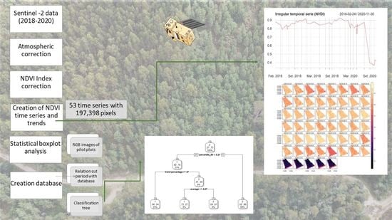
Multi-Temporal Sentinel-2 Data Analysis for Smallholding Forest Cut Control
Abstract
:1. Introduction
2. Materials and Methods
2.1. Study Area
2.2. Data Collection and Preprocessing
2.3. Normalized Difference Vegetation Index (NDVI)
2.4. Detection of the Forest Cutting Threshold
3. Results
3.1. Variation in NDVI
3.2. Detection of the Forest Cutting Threshold
4. Discussion
5. Conclusions
Author Contributions
Funding
Institutional Review Board Statement
Informed Consent Statement
Data Availability Statement
Acknowledgments
Conflicts of Interest
Appendix A
| Average | 25 th Percentile | 50th Percentile | 75th Percentile | 95th Percentile | Area(ha) | Perimeter (m) | Clear-Cut | Area Trend (ha) | Relation Index Descent Area—Stand Area (%) |
| −0.23877 | −0.31345 | −0.24974 | −0.16741 | −0.14145 | 0.063 | 189.26 | 1 | 0.06 | 95.24 |
| −0.14236 | −0.13783 | −0.13709 | −0.13009 | −0.1266 | 0.103 | 302.67 | 2 | 0.05 | 48.54 |
| −0.14921 | −0.14921 | −0.14921 | −0.14921 | −0.14921 | 0.18 | 235.27 | 2 | 0.01 | 5.56 |
| −0.2041 | −0.24096 | −0.19674 | −0.17645 | −0.1424 | 0.186 | 242.59 | 1 | 0.16 | 86.02 |
| −0.15906 | −0.17361 | −0.16287 | −0.1425 | −0.13619 | 0.194 | 348.14 | 2 | 0.07 | 36.08 |
| −0.35642 | −0.41328 | −0.35988 | −0.33433 | −0.25851 | 0.194 | 348.14 | 1 | 0.18 | 92.78 |
| −0.35454 | −0.39495 | −0.35508 | −0.31162 | −0.25826 | 0.202 | 260.5 | 1 | 0.19 | 94.06 |
| −0.15058 | −0.15058 | −0.15058 | −0.15058 | −0.15058 | 0.202 | 260.5 | 2 | 0.01 | 4.95 |
| −0.32099 | −0.36368 | −0.33208 | −0.29105 | −0.20624 | 0.204 | 387.59 | 1 | 0.2 | 98.04 |
| −0.17462 | −0.2024 | −0.16683 | −0.15611 | −0.13997 | 0.204 | 387.59 | 2 | 0.12 | 58.82 |
| −0.19082 | −0.2084 | −0.18672 | −0.13805 | −0.13523 | 0.204 | 387.59 | 2 | 0.05 | 24.51 |
| −0.16084 | −0.16588 | −0.16084 | −0.15579 | −0.15175 | 0.209 | 185.96 | 2 | 0.02 | 9.57 |
| −0.15295 | −0.16514 | −0.15532 | −0.13617 | −0.13004 | 0.219 | 500.02 | 2 | 0.06 | 27.4 |
| −0.34427 | −0.38731 | −0.33371 | −0.30781 | −0.27604 | 0.236 | 446.16 | 1 | 0.22 | 93.22 |
| −0.20902 | −0.20902 | −0.20902 | −0.20902 | −0.20902 | 0.236 | 446.16 | 2 | 0.01 | 4.24 |
| −0.20587 | −0.21751 | −0.20587 | −0.19422 | −0.1849 | 0.254 | 276.02 | 2 | 0.02 | 7.87 |
| −0.13207 | −0.13484 | −0.13207 | −0.12931 | −0.12709 | 0.254 | 276.02 | 2 | 0.02 | 7.87 |
| −0.35017 | −0.40293 | −0.38108 | −0.30716 | −0.18631 | 0.254 | 276.02 | 1 | 0.18 | 70.87 |
| −0.18862 | −0.18862 | −0.18862 | −0.18862 | −0.18862 | 0.254 | 276.02 | 2 | 0.01 | 3.94 |
| −0.22094 | −0.22225 | −0.22094 | −0.21962 | −0.21856 | 0.269 | 368.92 | 2 | 0.02 | 7.43 |
| −0.28922 | −0.32187 | −0.31068 | −0.25016 | −0.17622 | 0.269 | 368.92 | 1 | 0.16 | 59.48 |
| −0.12869 | −0.12995 | −0.12869 | −0.12742 | −0.12641 | 0.275 | 506.63 | 2 | 0.02 | 7.27 |
| −0.172 | −0.18233 | −0.172 | −0.16166 | −0.15339 | 0.275 | 506.63 | 2 | 0.02 | 7.27 |
| −0.12664 | −0.12664 | −0.12664 | −0.12664 | −0.12664 | 0.275 | 506.63 | 2 | 0.01 | 3.64 |
| −0.37358 | −0.42862 | −0.39838 | −0.37494 | −0.14041 | 0.275 | 506.63 | 1 | 0.19 | 69.09 |
| −0.23837 | −0.3046 | −0.26039 | −0.16894 | −0.14108 | 0.279 | 531.97 | 1 | 0.14 | 50.18 |
| −0.14238 | −0.14238 | −0.14238 | −0.14238 | −0.14238 | 0.295 | 587.95 | 2 | 0.01 | 3.39 |
| −0.14614 | −0.15365 | −0.14592 | −0.13547 | −0.13272 | 0.295 | 587.95 | 1 | 0.09 | 30.51 |
| −0.15319 | −0.16122 | −0.14954 | −0.14341 | −0.13602 | 0.364 | 252.12 | 2 | 0.07 | 19.23 |
| −0.14546 | −0.14617 | −0.14546 | −0.14476 | −0.14419 | 0.368 | 253.8 | 2 | 0.02 | 5.43 |
| −0.15973 | −0.16669 | −0.15339 | −0.14643 | −0.1411 | 0.38 | 270.81 | 2 | 0.04 | 10.53 |
| −0.4217 | −0.45081 | −0.42437 | −0.40781 | −0.36641 | 0.38 | 270.81 | 1 | 0.39 | 102.63 |
| −0.30046 | −0.33721 | −0.30511 | −0.27612 | −0.18231 | 0.383 | 248.68 | 1 | 0.29 | 75.72 |
| −0.14091 | −0.14793 | −0.13359 | −0.13088 | −0.13059 | 0.383 | 248.68 | 2 | 0.05 | 13.05 |
| −0.15896 | −0.17657 | −0.14134 | −0.13374 | −0.12871 | 0.39 | 309.34 | 2 | 0.07 | 17.95 |
| −0.14411 | −0.14516 | −0.14411 | −0.14306 | −0.14222 | 0.39 | 309.34 | 2 | 0.02 | 5.13 |
| −0.15863 | −0.17297 | −0.1497 | −0.14728 | −0.14414 | 0.39 | 309.34 | 1 | 0.05 | 12.82 |
| −0.16014 | −0.16014 | −0.16014 | −0.16014 | −0.16014 | 0.402 | 408.01 | 2 | 0.01 | 2.49 |
| −0.13443 | −0.13919 | −0.1341 | −0.12933 | −0.12783 | 0.402 | 408.01 | 2 | 0.04 | 9.95 |
| −0.15494 | −0.16401 | −0.15768 | −0.1472 | −0.13283 | 0.413 | 457.7 | 2 | 0.21 | 50.85 |
| −0.24233 | −0.29505 | −0.16709 | −0.14485 | −0.12801 | 0.413 | 457.7 | 1 | 0.31 | 75.06 |
| −0.27044 | −0.32025 | −0.29086 | −0.23921 | −0.13733 | 0.413 | 457.7 | 2 | 0.16 | 38.74 |
| −0.35753 | −0.39893 | −0.35753 | −0.31612 | −0.28299 | 0.415 | 689.22 | 2 | 0.02 | 4.82 |
| −0.234 | −0.27463 | −0.20422 | −0.15621 | −0.13366 | 0.415 | 689.22 | 2 | 0.36 | 86.75 |
| −0.35063 | −0.44136 | −0.35593 | −0.26473 | −0.17073 | 0.415 | 332.78 | 1 | 0.39 | 93.98 |
| −0.19055 | −0.20578 | −0.18382 | −0.16341 | −0.14216 | 0.453 | 320.27 | 2 | 0.11 | 24.28 |
| −0.20862 | −0.24305 | −0.21826 | −0.16955 | −0.14365 | 0.453 | 320.27 | 1 | 0.27 | 59.6 |
| −0.20522 | −0.22355 | −0.19334 | −0.1765 | −0.15971 | 0.462 | 502.26 | 2 | 0.07 | 15.15 |
| −0.15046 | −0.15215 | −0.15051 | −0.1488 | −0.14743 | 0.462 | 502.26 | 2 | 0.03 | 6.49 |
| −0.30753 | −0.38042 | −0.33914 | −0.21204 | −0.14985 | 0.462 | 502.26 | 1 | 0.29 | 62.77 |
| −0.3824 | −0.41636 | −0.40474 | −0.38373 | −0.22455 | 0.463 | 315.55 | 1 | 0.45 | 97.19 |
| −0.198 | −0.19826 | −0.198 | −0.19775 | −0.19754 | 0.463 | 315.55 | 2 | 0.02 | 4.32 |
| −0.15278 | −0.15278 | −0.15278 | −0.15278 | −0.15278 | 0.492 | 423.09 | 2 | 0.01 | 2.03 |
| −0.15099 | −0.16126 | −0.14946 | −0.13644 | −0.13032 | 0.492 | 423.09 | 2 | 0.25 | 50.81 |
| −0.29542 | −0.34644 | −0.29376 | −0.27071 | −0.191 | 0.492 | 423.09 | 1 | 0.46 | 93.5 |
| −0.16454 | −0.16454 | −0.16454 | −0.16454 | −0.16454 | 0.499 | 302.34 | 2 | 0.01 | 2 |
| −0.21635 | −0.26086 | −0.22876 | −0.16883 | −0.14041 | 0.522 | 302.47 | 1 | 0.35 | 67.05 |
| −0.16017 | −0.17618 | −0.16173 | −0.14332 | −0.13934 | 0.534 | 772.16 | 2 | 0.05 | 9.36 |
| −0.29322 | −0.32089 | −0.29705 | −0.26273 | −0.20361 | 0.551 | 433.42 | 1 | 0.49 | 88.93 |
| −0.13408 | −0.13488 | −0.13408 | −0.13327 | −0.13263 | 0.551 | 433.42 | 2 | 0.02 | 3.63 |
| −0.16567 | −0.18474 | −0.16381 | −0.14497 | −0.13705 | 0.577 | 504.69 | 2 | 0.1 | 17.33 |
| −0.24706 | −0.32224 | −0.25198 | −0.17758 | −0.1348 | 0.577 | 504.69 | 1 | 0.26 | 45.06 |
| −0.20405 | −0.25438 | −0.162 | −0.14291 | −0.12685 | 0.587 | 523.69 | 1 | 0.25 | 42.59 |
| −0.12965 | −0.12965 | −0.12965 | −0.12965 | −0.12965 | 0.587 | 523.69 | 2 | 0.01 | 1.7 |
| −0.21846 | −0.2488 | −0.23224 | −0.17683 | −0.16231 | 0.605 | 389.32 | 1 | 0.07 | 11.57 |
| −0.15958 | −0.15958 | −0.15958 | −0.15958 | −0.15958 | 0.605 | 389.32 | 2 | 0.01 | 1.65 |
| −0.16518 | −0.19373 | −0.15261 | −0.13244 | −0.12864 | 0.611 | 472.01 | 2 | 0.05 | 8.18 |
| −0.1471 | −0.14699 | −0.14561 | −0.14256 | −0.13308 | 0.611 | 472.01 | 2 | 0.09 | 14.73 |
| −0.15872 | −0.17026 | −0.15525 | −0.14544 | −0.13759 | 0.611 | 472.01 | 2 | 0.03 | 4.91 |
| −0.36968 | −0.41931 | −0.3967 | −0.33556 | −0.2194 | 0.611 | 472.01 | 1 | 0.29 | 47.46 |
| −0.16747 | −0.18176 | −0.17217 | −0.14669 | −0.13453 | 0.611 | 472.01 | 2 | 0.12 | 19.64 |
| −0.12948 | −0.12948 | −0.12948 | −0.12948 | −0.12948 | 0.614 | 315.79 | 2 | 0.01 | 1.63 |
| −0.22906 | −0.25549 | −0.22906 | −0.20262 | −0.18148 | 0.614 | 315.79 | 1 | 0.02 | 3.26 |
| −0.16531 | −0.17928 | −0.16814 | −0.14702 | −0.13407 | 0.614 | 315.79 | 2 | 0.1 | 16.29 |
| −0.14818 | −0.15221 | −0.14267 | −0.13863 | −0.1354 | 0.614 | 315.79 | 2 | 0.04 | 6.51 |
| −0.19836 | −0.19946 | −0.19836 | −0.19727 | −0.19639 | 0.619 | 431.28 | 2 | 0.02 | 3.23 |
| −0.24374 | −0.3085 | −0.23594 | −0.18562 | −0.13743 | 0.619 | 431.28 | 1 | 0.46 | 74.31 |
| −0.14678 | −0.1504 | −0.14678 | −0.14315 | −0.14025 | 0.619 | 431.28 | 2 | 0.02 | 3.23 |
| −0.1378 | −0.13947 | −0.13594 | −0.12972 | −0.12752 | 0.619 | 431.28 | 2 | 0.05 | 8.08 |
| −0.15093 | −0.15295 | −0.15093 | −0.1489 | −0.14728 | 0.619 | 431.28 | 2 | 0.02 | 3.23 |
| −0.30772 | −0.37153 | −0.31911 | −0.23704 | −0.17061 | 0.629 | 345.62 | 1 | 0.6 | 95.39 |
| −0.16679 | −0.18572 | −0.16075 | −0.13936 | −0.13491 | 0.629 | 345.62 | 2 | 0.08 | 12.72 |
| −0.14661 | −0.14661 | −0.14661 | −0.14661 | −0.14661 | 0.638 | 683.38 | 2 | 0.01 | 1.57 |
| −0.14974 | −0.17166 | −0.1389 | −0.1327 | −0.13226 | 0.638 | 683.38 | 2 | 0.05 | 7.84 |
| −0.21601 | −0.24116 | −0.22003 | −0.19058 | −0.15764 | 0.638 | 683.38 | 1 | 0.58 | 90.91 |
| −0.20602 | −0.22973 | −0.19779 | −0.17772 | −0.16139 | 0.668 | 343.15 | 1 | 0.12 | 17.96 |
| −0.17343 | −0.2169 | −0.15745 | −0.14348 | −0.12748 | 0.668 | 343.15 | 2 | 0.1 | 14.97 |
| −0.15988 | −0.17447 | −0.14973 | −0.1443 | −0.13853 | 0.668 | 343.15 | 2 | 0.08 | 11.98 |
| −0.17213 | −0.1877 | −0.18008 | −0.16451 | −0.13819 | 0.668 | 343.15 | 2 | 0.04 | 5.99 |
| −0.32665 | −0.3704 | −0.32236 | −0.29145 | −0.2461 | 0.692 | 435.44 | 1 | 0.72 | 104.05 |
| −0.22025 | −0.24663 | −0.22781 | −0.20284 | −0.14171 | 0.692 | 435.44 | 2 | 0.42 | 60.69 |
| −0.13173 | −0.13173 | −0.13173 | −0.13173 | −0.13173 | 0.707 | 360.16 | 2 | 0.01 | 1.41 |
| −0.41584 | −0.45852 | −0.44072 | −0.41877 | −0.21535 | 0.707 | 360.16 | 1 | 0.65 | 91.94 |
| −0.15118 | −0.1559 | −0.14022 | −0.13288 | −0.13137 | 0.71 | 412.36 | 2 | 0.05 | 7.04 |
| −0.33678 | −0.44056 | −0.32327 | −0.2454 | −0.15562 | 0.71 | 412.36 | 1 | 0.61 | 85.92 |
| −0.12591 | −0.12591 | −0.12591 | −0.12591 | −0.12591 | 0.715 | 359.9 | 2 | 0.01 | 1.4 |
| −0.14878 | −0.1542 | −0.14878 | −0.14335 | −0.13901 | 0.715 | 359.9 | 2 | 0.02 | 2.8 |
| −0.23194 | −0.26184 | −0.23153 | −0.21037 | −0.15156 | 0.715 | 359.9 | 1 | 0.44 | 61.54 |
| −0.14305 | −0.14305 | −0.14305 | −0.14305 | −0.14305 | 0.715 | 359.9 | 2 | 0.01 | 1.4 |
| −0.33401 | −0.40794 | −0.35568 | −0.278 | −0.15586 | 0.716 | 432.83 | 1 | 0.54 | 75.42 |
| −0.33509 | −0.41056 | −0.36944 | −0.26877 | −0.16603 | 0.746 | 462.69 | 1 | 0.51 | 68.36 |
| −0.17877 | −0.2117 | −0.1808 | −0.14591 | −0.1348 | 0.746 | 462.69 | 2 | 0.07 | 9.38 |
| −0.26115 | −0.31091 | −0.27793 | −0.21521 | −0.13916 | 0.748 | 544.1 | 1 | 0.65 | 86.9 |
| −0.19861 | −0.21322 | −0.19861 | −0.18401 | −0.17232 | 0.748 | 544.1 | 2 | 0.02 | 2.67 |
| −0.20047 | −0.23462 | −0.19901 | −0.1694 | −0.1352 | 0.748 | 544.1 | 2 | 0.3 | 40.11 |
| −0.30514 | −0.34035 | −0.31851 | −0.28212 | −0.20341 | 0.765 | 444.89 | 1 | 0.71 | 92.81 |
| −0.13666 | −0.13892 | −0.13546 | −0.1338 | −0.13247 | 0.765 | 444.89 | 2 | 0.03 | 3.92 |
| −0.38992 | −0.48775 | −0.41262 | −0.31138 | −0.16222 | 0.769 | 411.84 | 1 | 0.69 | 89.73 |
| −0.14309 | −0.15088 | −0.14352 | −0.13573 | −0.12897 | 0.769 | 411.84 | 2 | 0.04 | 5.2 |
| −0.16355 | −0.16911 | −0.16717 | −0.1598 | −0.1539 | 0.769 | 411.84 | 2 | 0.03 | 3.9 |
| −0.40813 | −0.46684 | −0.43483 | −0.39507 | −0.22932 | 0.773 | 362.02 | 1 | 0.7 | 90.56 |
| −0.16374 | −0.17565 | −0.17277 | −0.15892 | −0.13462 | 0.773 | 362.02 | 2 | 0.09 | 11.64 |
| −0.17646 | −0.19277 | −0.14431 | −0.14408 | −0.1439 | 0.773 | 362.02 | 2 | 0.03 | 3.88 |
| −0.19216 | −0.20802 | −0.18749 | −0.16387 | −0.14497 | 0.773 | 362.02 | 2 | 0.11 | 14.23 |
| −0.32543 | −0.40899 | −0.3326 | −0.24832 | −0.16265 | 0.791 | 462.16 | 1 | 0.64 | 80.91 |
| −0.17959 | −0.19274 | −0.18529 | −0.15754 | −0.13686 | 0.791 | 462.16 | 2 | 0.17 | 21.49 |
| −0.17452 | −0.20626 | −0.15164 | −0.13981 | −0.13626 | 0.791 | 462.16 | 2 | 0.11 | 13.91 |
| −0.13942 | −0.14315 | −0.13962 | −0.13579 | −0.13273 | 0.791 | 462.16 | 2 | 0.03 | 3.79 |
| −0.15858 | −0.15858 | −0.15858 | −0.15858 | −0.15858 | 0.791 | 462.16 | 2 | 0.01 | 1.26 |
| −0.16151 | −0.17943 | −0.16919 | −0.14743 | −0.13002 | 0.791 | 462.16 | 2 | 0.03 | 3.79 |
| −0.17818 | −0.2009 | −0.17053 | −0.15725 | −0.14602 | 0.795 | 356.79 | 2 | 0.07 | 8.81 |
| −0.18881 | −0.21064 | −0.17243 | −0.15773 | −0.13437 | 0.795 | 356.79 | 2 | 0.1 | 12.58 |
| −0.13971 | −0.14571 | −0.14383 | −0.13577 | −0.12932 | 0.821 | 361.93 | 2 | 0.03 | 3.65 |
| −0.2252 | −0.26877 | −0.21795 | −0.18538 | −0.135 | 0.821 | 361.93 | 1 | 0.68 | 82.83 |
| −0.14697 | −0.15684 | −0.12913 | −0.12819 | −0.12744 | 0.821 | 361.93 | 2 | 0.03 | 3.65 |
| −0.14155 | −0.14333 | −0.14155 | −0.13976 | −0.13834 | 0.821 | 361.93 | 2 | 0.02 | 2.44 |
| −0.23558 | −0.27408 | −0.23837 | −0.19542 | −0.14678 | 0.823 | 452.19 | 1 | 0.61 | 74.12 |
| −0.13668 | −0.14003 | −0.13807 | −0.1336 | −0.1304 | 0.823 | 452.19 | 2 | 0.07 | 8.51 |
| −0.27042 | −0.30374 | −0.27551 | −0.23732 | −0.18075 | 0.861 | 440.34 | 1 | 0.76 | 88.27 |
| −0.12693 | −0.12693 | −0.12693 | −0.12693 | −0.12693 | 0.876 | 390.47 | 2 | 0.01 | 1.14 |
| −0.13706 | −0.13706 | −0.13706 | −0.13706 | −0.13706 | 0.876 | 390.47 | 2 | 0.01 | 1.14 |
| −0.32596 | −0.4188 | −0.37254 | −0.23004 | −0.1688 | 0.876 | 390.47 | 1 | 0.44 | 50.23 |
| −0.20173 | −0.21917 | −0.19154 | −0.1792 | −0.16933 | 0.886 | 467.32 | 2 | 0.03 | 3.39 |
| −0.35299 | −0.45323 | −0.35731 | −0.26468 | −0.16272 | 0.886 | 467.32 | 1 | 0.68 | 76.75 |
| −0.18605 | −0.22464 | −0.14717 | −0.13747 | −0.1317 | 0.886 | 467.32 | 2 | 0.11 | 12.42 |
| −0.19481 | −0.23776 | −0.19167 | −0.15523 | −0.13802 | 0.886 | 467.32 | 2 | 0.23 | 25.96 |
| −0.1572 | −0.1572 | −0.1572 | −0.1572 | −0.1572 | 0.886 | 467.32 | 2 | 0.01 | 1.13 |
| −0.30398 | −0.34898 | −0.31487 | −0.27458 | −0.18144 | 0.9 | 455.27 | 1 | 0.83 | 92.22 |
| −0.2989 | −0.34883 | −0.29243 | −0.24718 | −0.19363 | 0.9 | 455.27 | 2 | 0.42 | 46.67 |
| −0.12757 | −0.12757 | −0.12757 | −0.12757 | −0.12757 | 0.9 | 455.27 | 2 | 0.01 | 1.11 |
| −0.22628 | −0.24534 | −0.23713 | −0.21807 | −0.18761 | 0.9 | 455.27 | 2 | 0.04 | 4.44 |
| −0.27436 | −0.34514 | −0.26262 | −0.2139 | −0.14133 | 0.908 | 511.18 | 1 | 0.83 | 91.41 |
| −0.16442 | −0.17681 | −0.16442 | −0.15204 | −0.14213 | 0.908 | 511.18 | 2 | 0.02 | 2.2 |
| −0.16197 | −0.1764 | −0.16096 | −0.13763 | −0.12823 | 0.913 | 448.16 | 2 | 0.29 | 31.76 |
| −0.15498 | −0.16496 | −0.16335 | −0.14919 | −0.13786 | 0.913 | 448.16 | 2 | 0.03 | 3.29 |
| −0.41859 | −0.46664 | −0.45126 | −0.40822 | −0.28365 | 0.918 | 458.24 | 2 | 0.23 | 25.05 |
| −0.14989 | −0.15397 | −0.14989 | −0.1458 | −0.14253 | 0.918 | 458.24 | 2 | 0.02 | 2.18 |
| −0.17522 | −0.19846 | −0.17145 | −0.15766 | −0.14598 | 0.918 | 458.24 | 2 | 0.08 | 8.71 |
| −0.2094 | −0.23321 | −0.22906 | −0.19543 | −0.16852 | 0.918 | 458.24 | 2 | 0.03 | 3.27 |
| −0.17523 | −0.19103 | −0.1748 | −0.15665 | −0.13807 | 0.918 | 458.24 | 2 | 0.27 | 29.41 |
| −0.13903 | −0.14348 | −0.13722 | −0.13368 | −0.13084 | 0.918 | 458.24 | 2 | 0.03 | 3.27 |
| −0.19098 | −0.20797 | −0.19111 | −0.17328 | −0.1395 | 0.918 | 458.24 | 1 | 0.24 | 26.14 |
| −0.15849 | −0.1713 | −0.15315 | −0.14302 | −0.13492 | 0.943 | 710.25 | 2 | 0.03 | 3.18 |
| −0.14374 | −0.14787 | −0.14374 | −0.13961 | −0.13631 | 0.943 | 710.25 | 2 | 0.02 | 2.12 |
| −0.33153 | −0.39665 | −0.32818 | −0.28573 | −0.18487 | 0.943 | 710.25 | 1 | 0.55 | 58.32 |
| −0.15729 | −0.16219 | −0.14834 | −0.12958 | −0.12601 | 0.943 | 710.25 | 2 | 0.11 | 11.66 |
| −0.15294 | −0.14484 | −0.13384 | −0.12997 | −0.12704 | 0.943 | 710.25 | 2 | 0.11 | 11.66 |
| −0.14583 | −0.14583 | −0.14583 | −0.14583 | −0.14583 | 0.962 | 418.73 | 2 | 0.01 | 1.04 |
| −0.40231 | −0.47654 | −0.44329 | −0.37441 | −0.1743 | 0.962 | 418.73 | 1 | 0.78 | 81.08 |
| −0.12961 | −0.12961 | −0.12961 | −0.12961 | −0.12961 | 0.962 | 418.73 | 2 | 0.01 | 1.04 |
| −0.22111 | −0.23154 | −0.22111 | −0.21067 | −0.20233 | 0.962 | 418.73 | 2 | 0.02 | 2.08 |
| −0.14114 | −0.14847 | −0.14137 | −0.13182 | −0.12788 | 0.962 | 418.73 | 2 | 0.14 | 14.55 |
| −0.27336 | −0.31871 | −0.2918 | −0.25483 | −0.15325 | 0.962 | 418.73 | 2 | 0.21 | 21.83 |
| −0.38266 | −0.41375 | −0.38909 | −0.37212 | −0.25544 | 0.984 | 689.22 | 1 | 0.99 | 100.61 |
| −0.14676 | −0.14676 | −0.14676 | −0.14676 | −0.14676 | 0.984 | 689.22 | 2 | 0.01 | 1.02 |
| −0.15851 | −0.16857 | −0.15851 | −0.14844 | −0.14038 | 0.984 | 689.22 | 2 | 0.02 | 2.03 |
| −0.17792 | −0.17792 | −0.17792 | −0.17792 | −0.17792 | 0.984 | 689.22 | 2 | 0.01 | 1.02 |
| −0.14446 | −0.14621 | −0.14184 | −0.13858 | −0.1317 | 0.996 | 477.71 | 2 | 0.16 | 16.06 |
| −0.35946 | −0.41441 | −0.35596 | −0.31942 | −0.28651 | 0.996 | 477.71 | 1 | 0.05 | 5.02 |
| −0.34873 | −0.43569 | −0.39303 | −0.27798 | −0.14455 | 1.006 | 638.79 | 1 | 0.81 | 80.52 |
| −0.12544 | −0.12544 | −0.12544 | −0.12544 | −0.12544 | 1.006 | 638.79 | 2 | 0.01 | 0.99 |
| −0.18772 | −0.18772 | −0.18772 | −0.18772 | −0.18772 | 1.006 | 638.79 | 2 | 0.01 | 0.99 |
| −0.18438 | −0.20876 | −0.18311 | −0.15051 | −0.12933 | 1.006 | 638.79 | 2 | 0.19 | 18.89 |
| −0.16488 | −0.1787 | −0.15481 | −0.1347 | −0.13071 | 1.006 | 638.79 | 2 | 0.1 | 9.94 |
| −0.17401 | −0.19803 | −0.17732 | −0.14536 | −0.13059 | 1.006 | 638.79 | 2 | 0.23 | 22.86 |
| −0.14198 | −0.14198 | −0.14198 | −0.14198 | −0.14198 | 1.006 | 638.79 | 2 | 0.01 | 0.99 |
| −0.1569 | −0.16131 | −0.15245 | −0.14804 | −0.13986 | 1.006 | 638.79 | 2 | 0.04 | 3.98 |
| −0.14617 | −0.1543 | −0.14617 | −0.13804 | −0.13154 | 1.006 | 638.79 | 2 | 0.02 | 1.99 |
| −0.15406 | −0.15406 | −0.15406 | −0.15406 | −0.15406 | 1.008 | 400.03 | 2 | 0.01 | 0.99 |
| −0.18067 | −0.18067 | −0.18067 | −0.18067 | −0.18067 | 1.008 | 400.03 | 2 | 0.01 | 0.99 |
| −0.25052 | −0.32763 | −0.24137 | −0.1525 | −0.12659 | 1.008 | 400.03 | 1 | 0.21 | 20.83 |
| −0.14487 | −0.1482 | −0.13723 | −0.13482 | −0.12823 | 1.008 | 400.03 | 2 | 0.09 | 8.93 |
| −0.16071 | −0.16336 | −0.15853 | −0.15588 | −0.15476 | 1.008 | 400.03 | 2 | 0.04 | 3.97 |
| −0.14141 | −0.14847 | −0.12867 | −0.12798 | −0.12742 | 1.008 | 400.03 | 2 | 0.03 | 2.98 |
| −0.14333 | −0.1456 | −0.14389 | −0.14135 | −0.13931 | 1.017 | 427.96 | 2 | 0.03 | 2.95 |
| −0.2278 | −0.26249 | −0.23562 | −0.18829 | −0.15082 | 1.017 | 427.96 | 1 | 0.61 | 59.98 |
| −0.15469 | −0.16526 | −0.152 | −0.138 | −0.13083 | 1.017 | 427.96 | 2 | 0.24 | 23.6 |
| −0.14555 | −0.15868 | −0.14004 | −0.13363 | −0.13076 | 1.017 | 427.96 | 2 | 0.08 | 7.87 |
| −0.1718 | −0.18515 | −0.17864 | −0.15001 | −0.13987 | 1.017 | 427.96 | 2 | 0.08 | 7.87 |
| −0.33715 | −0.40961 | −0.32745 | −0.26418 | −0.15354 | 1.019 | 467.94 | 1 | 0.98 | 96.17 |
| −0.15995 | −0.16928 | −0.15396 | −0.14269 | −0.13495 | 1.019 | 467.94 | 2 | 0.1 | 9.81 |
| −0.15515 | −0.16715 | −0.15093 | −0.14012 | −0.1302 | 1.026 | 403.8 | 2 | 0.11 | 10.72 |
| −0.14079 | −0.14079 | −0.14079 | −0.14079 | −0.14079 | 1.026 | 403.8 | 2 | 0.01 | 0.97 |
| −0.14064 | −0.14064 | −0.14064 | −0.14064 | −0.14064 | 1.026 | 403.8 | 2 | 0.01 | 0.97 |
| −0.29391 | −0.36428 | −0.28989 | −0.22696 | −0.15581 | 1.038 | 579.92 | 1 | 0.28 | 26.97 |
| −0.23074 | −0.25826 | −0.22853 | −0.19238 | −0.14115 | 1.048 | 529.15 | 1 | 0.84 | 80.15 |
| −0.12824 | −0.12824 | −0.12824 | −0.12824 | −0.12824 | 1.048 | 529.15 | 2 | 0.01 | 0.95 |
| −0.21239 | −0.25105 | −0.21075 | −0.17251 | −0.14032 | 1.061 | 474.72 | 1 | 0.93 | 87.65 |
| −0.2477 | −0.3118 | −0.245 | −0.19237 | −0.1346 | 1.075 | 450.52 | 1 | 0.59 | 54.88 |
| −0.13342 | −0.13536 | −0.13342 | −0.13149 | −0.12994 | 1.075 | 450.52 | 2 | 0.02 | 1.86 |
| −0.15088 | −0.157 | −0.14437 | −0.13798 | −0.12863 | 1.075 | 450.52 | 2 | 0.33 | 30.7 |
| −0.13013 | −0.13013 | −0.13013 | −0.13013 | −0.13013 | 1.075 | 450.52 | 2 | 0.01 | 0.93 |
| −0.20505 | −0.26001 | −0.19054 | −0.15428 | −0.1381 | 1.075 | 450.52 | 2 | 0.1 | 9.3 |
| −0.16455 | −0.16455 | −0.16455 | −0.16455 | −0.16455 | 1.089 | 474.39 | 2 | 0.01 | 0.92 |
| −0.48956 | −0.53617 | −0.51696 | −0.48819 | −0.26834 | 1.089 | 474.39 | 1 | 1.05 | 96.42 |
| −0.2871 | −0.34301 | −0.29311 | −0.2297 | −0.14911 | 1.097 | 761.25 | 1 | 0.98 | 89.33 |
| −0.13857 | −0.14033 | −0.13857 | −0.13682 | −0.13541 | 1.097 | 761.25 | 2 | 0.02 | 1.82 |
| −0.24232 | −0.28211 | −0.2513 | −0.21288 | −0.15023 | 1.102 | 466.63 | 2 | 0.99 | 89.84 |
| −0.2712 | −0.31745 | −0.269 | −0.23001 | −0.15991 | 1.102 | 466.63 | 1 | 0.99 | 89.84 |
| −0.14535 | −0.14535 | −0.14535 | −0.14535 | −0.14535 | 1.102 | 466.63 | 2 | 0.01 | 0.91 |
| −0.15925 | −0.15925 | −0.15925 | −0.15925 | −0.15925 | 1.102 | 466.63 | 2 | 0.01 | 0.91 |
| −0.13492 | −0.13495 | −0.13492 | −0.13488 | −0.13486 | 1.102 | 466.63 | 2 | 0.02 | 1.81 |
| −0.13239 | −0.13572 | −0.13241 | −0.12907 | −0.12639 | 1.108 | 488.13 | 2 | 0.03 | 2.71 |
| −0.48828 | −0.5628 | −0.52159 | −0.45329 | −0.22244 | 1.108 | 488.13 | 1 | 1.09 | 98.38 |
| −0.13775 | −0.13775 | −0.13775 | −0.13775 | −0.13775 | 1.117 | 752 | 2 | 0.01 | 0.9 |
| −0.14683 | −0.15524 | −0.14683 | −0.13841 | −0.13168 | 1.117 | 752 | 2 | 0.02 | 1.79 |
| −0.33481 | −0.36989 | −0.34567 | −0.31139 | −0.22684 | 1.117 | 752 | 1 | 1.13 | 101.16 |
| −0.13514 | −0.13514 | −0.13514 | −0.13514 | −0.13514 | 1.117 | 752 | 2 | 0.01 | 0.9 |
| −0.15641 | −0.16981 | −0.16895 | −0.14929 | −0.13355 | 1.177 | 448.82 | 2 | 0.03 | 2.55 |
| −0.15435 | −0.15333 | −0.14336 | −0.12951 | −0.12811 | 1.177 | 448.82 | 2 | 0.05 | 4.25 |
| −0.22617 | −0.26021 | −0.22781 | −0.19598 | −0.13337 | 1.177 | 448.82 | 1 | 1.06 | 90.06 |
| −0.1503 | −0.1503 | −0.1503 | −0.1503 | −0.1503 | 1.177 | 448.82 | 2 | 0.01 | 0.85 |
| −0.16354 | −0.18519 | −0.16598 | −0.1495 | −0.13137 | 1.177 | 448.82 | 2 | 0.05 | 4.25 |
| −0.21924 | −0.31437 | −0.17139 | −0.15599 | −0.13296 | 1.177 | 448.82 | 2 | 0.1 | 8.5 |
| −0.1489 | −0.16752 | −0.13855 | −0.12969 | −0.12645 | 1.244 | 507.63 | 2 | 0.36 | 28.94 |
| −0.15502 | −0.163 | −0.15071 | −0.14086 | −0.13324 | 1.244 | 507.63 | 2 | 0.18 | 14.47 |
| −0.13694 | −0.13809 | −0.13694 | −0.1358 | −0.13488 | 1.247 | 501.95 | 2 | 0.02 | 1.6 |
| −0.42585 | −0.47734 | −0.42778 | −0.39049 | −0.30692 | 1.247 | 501.95 | 1 | 1.22 | 97.83 |
| −0.29315 | −0.33941 | −0.30152 | −0.24793 | −0.16824 | 1.253 | 654.51 | 2 | 0.85 | 67.84 |
| −0.15036 | −0.15588 | −0.15036 | −0.14483 | −0.14041 | 1.253 | 654.51 | 2 | 0.02 | 1.6 |
| −0.20444 | −0.24331 | −0.19627 | −0.16347 | −0.13641 | 1.253 | 654.51 | 1 | 0.59 | 47.09 |
| −0.14777 | −0.15588 | −0.14586 | −0.13894 | −0.13109 | 1.253 | 654.51 | 2 | 0.06 | 4.79 |
| −0.14255 | −0.14455 | −0.13985 | −0.13921 | −0.13869 | 1.253 | 654.51 | 2 | 0.03 | 2.39 |
| −0.16998 | −0.17876 | −0.1688 | −0.15795 | −0.13982 | 1.254 | 595.13 | 2 | 0.06 | 4.78 |
| −0.24141 | −0.28362 | −0.23381 | −0.18437 | −0.1402 | 1.254 | 595.13 | 1 | 0.35 | 27.91 |
| −0.12587 | −0.12587 | −0.12587 | −0.12587 | −0.12587 | 1.254 | 595.13 | 2 | 0.01 | 0.8 |
| −0.1388 | −0.1388 | −0.1388 | −0.1388 | −0.1388 | 1.254 | 595.13 | 2 | 0.01 | 0.8 |
| −0.15553 | −0.16958 | −0.16827 | −0.14785 | −0.13151 | 1.254 | 595.13 | 2 | 0.03 | 2.39 |
| −0.26 | −0.31648 | −0.27511 | −0.1715 | −0.13074 | 1.298 | 454.85 | 1 | 0.94 | 72.42 |
| −0.13227 | −0.13227 | −0.13227 | −0.13227 | −0.13227 | 1.298 | 454.85 | 2 | 0.01 | 0.77 |
| −0.14447 | −0.15416 | −0.14141 | −0.13172 | −0.12889 | 1.298 | 454.85 | 2 | 0.04 | 3.08 |
| −0.14907 | −0.16029 | −0.14752 | −0.13707 | −0.12871 | 1.307 | 482.94 | 2 | 0.03 | 2.3 |
| −0.15046 | −0.16548 | −0.14698 | −0.12761 | −0.12672 | 1.307 | 482.94 | 2 | 0.06 | 4.59 |
| −0.20973 | −0.23732 | −0.19871 | −0.18646 | −0.14718 | 1.307 | 482.94 | 2 | 0.3 | 22.95 |
| −0.3389 | −0.4469 | −0.39513 | −0.21973 | −0.14023 | 1.307 | 482.94 | 1 | 0.82 | 62.74 |
| −0.2197 | −0.2525 | −0.21202 | −0.1867 | −0.13882 | 1.386 | 477.89 | 1 | 0.99 | 71.43 |
| −0.14198 | −0.14198 | −0.14198 | −0.14198 | −0.14198 | 1.386 | 477.89 | 2 | 0.01 | 0.72 |
| −0.17832 | −0.1791 | −0.17832 | −0.17755 | −0.17693 | 1.4 | 905.49 | 2 | 0.02 | 1.43 |
| −0.34794 | −0.40323 | −0.38166 | −0.31765 | −0.18922 | 1.4 | 905.49 | 1 | 1.41 | 100.71 |
| −0.12593 | −0.12593 | −0.12593 | −0.12593 | −0.12593 | 1.4 | 905.49 | 2 | 0.01 | 0.71 |
| −0.14346 | −0.15575 | −0.13949 | −0.13506 | −0.12854 | 1.414 | 604.32 | 2 | 0.05 | 3.54 |
| −0.14042 | −0.14652 | −0.13546 | −0.12928 | −0.12783 | 1.414 | 604.32 | 2 | 0.06 | 4.24 |
| −0.15487 | −0.16991 | −0.15149 | −0.14325 | −0.1298 | 1.414 | 604.32 | 2 | 0.36 | 25.46 |
| −0.14767 | −0.14767 | −0.14767 | −0.14767 | −0.14767 | 1.459 | 606.09 | 2 | 0.01 | 0.69 |
| −0.1387 | −0.14234 | −0.13889 | −0.13525 | −0.12904 | 1.459 | 639.78 | 2 | 0.04 | 2.74 |
| −0.14667 | −0.15867 | −0.14224 | −0.13062 | −0.12641 | 1.459 | 606.09 | 2 | 0.24 | 16.45 |
| −0.14097 | −0.14097 | −0.14097 | −0.14097 | −0.14097 | 1.459 | 639.78 | 2 | 0.01 | 0.69 |
| −0.12671 | −0.12671 | −0.12671 | −0.12671 | −0.12671 | 1.459 | 606.09 | 2 | 0.01 | 0.69 |
| −0.15664 | −0.16191 | −0.15274 | −0.13665 | −0.13007 | 1.459 | 606.09 | 2 | 0.14 | 9.6 |
| −0.20327 | −0.23658 | −0.19115 | −0.16263 | −0.13083 | 1.459 | 606.09 | 1 | 0.21 | 14.39 |
| −0.34267 | −0.41808 | −0.37392 | −0.27596 | −0.1836 | 1.459 | 639.78 | 1 | 1.3 | 89.1 |
| −0.35398 | −0.41715 | −0.37863 | −0.3037 | −0.20019 | 1.476 | 683.82 | 1 | 1.47 | 99.59 |
| −0.13755 | −0.14252 | −0.14027 | −0.13394 | −0.12887 | 1.476 | 683.82 | 2 | 0.03 | 2.03 |
| −0.14533 | −0.15132 | −0.14997 | −0.14167 | −0.13503 | 1.5 | 733.89 | 2 | 0.03 | 2 |
| −0.1468 | −0.1518 | −0.1468 | −0.14181 | −0.13781 | 1.5 | 733.89 | 2 | 0.02 | 1.33 |
| −0.13751 | −0.13751 | −0.13751 | −0.13751 | −0.13751 | 1.5 | 733.89 | 2 | 0.01 | 0.67 |
| −0.14023 | −0.14023 | −0.14023 | −0.14023 | −0.14023 | 1.501 | 545.61 | 2 | 0.01 | 0.67 |
| −0.13245 | −0.13245 | −0.13245 | −0.13245 | −0.13245 | 1.601 | 521.45 | 2 | 0.01 | 0.62 |
| −0.1379 | −0.1379 | −0.1379 | −0.1379 | −0.1379 | 1.601 | 521.45 | 2 | 0.01 | 0.62 |
| −0.16961 | −0.1781 | −0.15739 | −0.14814 | −0.1302 | 1.601 | 521.45 | 2 | 0.26 | 16.24 |
| −0.15795 | −0.16553 | −0.15394 | −0.14921 | −0.1341 | 1.601 | 521.45 | 2 | 0.13 | 8.12 |
| −0.21458 | −0.24177 | −0.22215 | −0.18569 | −0.13197 | 1.601 | 521.45 | 1 | 0.89 | 55.59 |
| −0.18542 | −0.21524 | −0.18213 | −0.15903 | −0.1423 | 1.635 | 554.6 | 2 | 0.25 | 15.29 |
| −0.14444 | −0.14444 | −0.14444 | −0.14444 | −0.14444 | 1.635 | 554.6 | 2 | 0.01 | 0.61 |
| −0.15267 | −0.15817 | −0.15136 | −0.14126 | −0.13561 | 1.635 | 554.6 | 2 | 0.06 | 3.67 |
| −0.21716 | −0.25869 | −0.20498 | −0.16668 | −0.13708 | 1.635 | 554.6 | 2 | 0.83 | 50.76 |
| −0.15287 | −0.15985 | −0.15117 | −0.14635 | −0.14072 | 1.635 | 554.6 | 2 | 0.05 | 3.06 |
| −0.21835 | −0.26563 | −0.22286 | −0.16413 | −0.1319 | 1.635 | 554.6 | 1 | 0.25 | 15.29 |
| −0.29059 | −0.33333 | −0.30054 | −0.26215 | −0.158 | 1.655 | 606.03 | 1 | 1.48 | 89.43 |
| −0.15938 | −0.17455 | −0.15357 | −0.14501 | −0.13479 | 1.655 | 606.03 | 2 | 0.06 | 3.63 |
| −0.15892 | −0.17544 | −0.15133 | −0.13647 | −0.13053 | 1.655 | 606.03 | 2 | 0.47 | 28.4 |
| −0.16947 | −0.16947 | −0.16947 | −0.16947 | −0.16947 | 1.667 | 507.11 | 2 | 0.01 | 0.6 |
| −0.14399 | −0.15113 | −0.14399 | −0.13685 | −0.13114 | 1.667 | 507.11 | 2 | 0.02 | 1.2 |
| −0.19546 | −0.24344 | −0.17814 | −0.14742 | −0.13883 | 1.667 | 507.11 | 2 | 0.06 | 3.6 |
| −0.14766 | −0.15024 | −0.14766 | −0.14507 | −0.143 | 1.723 | 678.92 | 2 | 0.02 | 1.16 |
| −0.1584 | −0.17022 | −0.14619 | −0.13219 | −0.12643 | 1.723 | 678.92 | 2 | 0.86 | 49.91 |
| −0.13257 | −0.13461 | −0.13288 | −0.13068 | −0.12892 | 1.723 | 678.92 | 2 | 0.03 | 1.74 |
| −0.13169 | −0.13169 | −0.13169 | −0.13169 | −0.13169 | 1.723 | 678.92 | 2 | 0.01 | 0.58 |
| −0.18098 | −0.18154 | −0.18098 | −0.18041 | −0.17996 | 1.723 | 678.92 | 2 | 0.02 | 1.16 |
| −0.14107 | −0.14878 | −0.12929 | −0.1279 | −0.12598 | 1.723 | 678.92 | 2 | 0.06 | 3.48 |
| −0.21704 | −0.24281 | −0.21843 | −0.19391 | −0.13694 | 1.723 | 678.92 | 1 | 1.63 | 94.6 |
| −0.14814 | −0.14814 | −0.14814 | −0.14814 | −0.14814 | 1.724 | 506.48 | 2 | 0.01 | 0.58 |
| −0.13965 | −0.13965 | −0.13965 | −0.13965 | −0.13965 | 1.724 | 506.48 | 2 | 0.01 | 0.58 |
| −0.35562 | −0.41459 | −0.37857 | −0.32367 | −0.17834 | 1.724 | 506.48 | 1 | 1.57 | 91.07 |
| −0.12671 | −0.12671 | −0.12671 | −0.12671 | −0.12671 | 1.724 | 506.48 | 2 | 0.01 | 0.58 |
| −0.13364 | −0.13364 | −0.13364 | −0.13364 | −0.13364 | 1.724 | 506.48 | 2 | 0.01 | 0.58 |
| −0.1421 | −0.14817 | −0.14124 | −0.13316 | −0.12655 | 1.724 | 506.48 | 2 | 0.65 | 37.7 |
| −0.25479 | −0.30969 | −0.25084 | −0.18642 | −0.14496 | 1.766 | 953.43 | 1 | 1.14 | 64.55 |
| −0.23973 | −0.2695 | −0.24759 | −0.21446 | −0.17215 | 1.812 | 623.92 | 1 | 0.43 | 23.73 |
| −0.16133 | −0.16133 | −0.16133 | −0.16133 | −0.16133 | 1.812 | 623.92 | 2 | 0.01 | 0.55 |
| −0.14372 | −0.15016 | −0.14372 | −0.13729 | −0.13214 | 1.812 | 623.92 | 2 | 0.02 | 1.1 |
| −0.27356 | −0.34141 | −0.2691 | −0.20169 | −0.14752 | 1.829 | 579.64 | 2 | 0.58 | 31.71 |
| −0.15457 | −0.16998 | −0.13838 | −0.12976 | −0.12683 | 1.829 | 579.64 | 2 | 0.14 | 7.65 |
| −0.21968 | −0.25895 | −0.21919 | −0.17942 | −0.13387 | 1.829 | 579.64 | 1 | 1.16 | 63.42 |
| −0.13046 | −0.13046 | −0.13046 | −0.13046 | −0.13046 | 1.831 | 571.67 | 2 | 0.01 | 0.55 |
| −0.14231 | −0.14954 | −0.14633 | −0.1371 | −0.12971 | 1.831 | 571.67 | 2 | 0.03 | 1.64 |
| −0.27859 | −0.39149 | −0.24764 | −0.1722 | −0.14462 | 1.831 | 571.67 | 1 | 1.51 | 82.47 |
| −0.17359 | −0.20475 | −0.17514 | −0.1361 | −0.1282 | 1.831 | 571.67 | 2 | 0.18 | 9.83 |
| −0.14677 | −0.14741 | −0.14677 | −0.14613 | −0.14562 | 1.855 | 624.87 | 2 | 0.02 | 1.08 |
| −0.23404 | −0.28065 | −0.23151 | −0.17762 | −0.13931 | 1.855 | 624.87 | 1 | 1.24 | 66.85 |
| −0.23753 | −0.26188 | −0.24376 | −0.22396 | −0.155 | 1.879 | 600.57 | 1 | 1.61 | 85.68 |
| −0.13107 | −0.13107 | −0.13107 | −0.13107 | −0.13107 | 1.879 | 600.57 | 2 | 0.01 | 0.53 |
| −0.1435 | −0.14644 | −0.13951 | −0.13263 | −0.13081 | 1.888 | 602.28 | 2 | 0.11 | 5.83 |
| −0.13331 | −0.1358 | −0.13331 | −0.13081 | −0.12882 | 1.888 | 602.28 | 2 | 0.02 | 1.06 |
| −0.40585 | −0.45969 | −0.42615 | −0.38028 | −0.21548 | 1.899 | 602.45 | 1 | 1.85 | 97.42 |
| −0.17522 | −0.21841 | −0.15497 | −0.13357 | −0.12836 | 1.899 | 602.45 | 2 | 0.21 | 11.06 |
| −0.14316 | −0.14316 | −0.14316 | −0.14316 | −0.14316 | 1.899 | 602.45 | 2 | 0.01 | 0.53 |
| −0.22906 | −0.24988 | −0.21584 | −0.19501 | −0.15383 | 1.899 | 602.45 | 2 | 0.04 | 2.11 |
| −0.13006 | −0.13006 | −0.13006 | −0.13006 | −0.13006 | 1.899 | 602.45 | 2 | 0.01 | 0.53 |
| −0.21874 | −0.23649 | −0.20481 | −0.1736 | −0.14765 | 1.903 | 593.22 | 2 | 0.3 | 15.76 |
| −0.26504 | −0.29645 | −0.27324 | −0.23117 | −0.15774 | 1.903 | 593.22 | 1 | 1.56 | 81.98 |
| −0.16172 | −0.16642 | −0.16172 | −0.15701 | −0.15325 | 1.903 | 593.22 | 2 | 0.02 | 1.05 |
| −0.15651 | −0.17117 | −0.15099 | −0.13909 | −0.12957 | 1.903 | 593.22 | 2 | 0.03 | 1.58 |
| −0.14408 | −0.14408 | −0.14408 | −0.14408 | −0.14408 | 1.903 | 593.22 | 2 | 0.01 | 0.53 |
| −0.2802 | −0.31621 | −0.28764 | −0.26531 | −0.15291 | 1.905 | 1208.87 | 2 | 0.43 | 22.57 |
| −0.21117 | −0.25255 | −0.18013 | −0.12749 | −0.12665 | 1.905 | 1208.87 | 2 | 0.05 | 2.62 |
| −0.16839 | −0.18316 | −0.16214 | −0.14968 | −0.14226 | 1.918 | 580.19 | 2 | 0.07 | 3.65 |
| −0.14233 | −0.14324 | −0.13267 | −0.13176 | −0.13116 | 1.918 | 580.19 | 2 | 0.04 | 2.09 |
| −0.35707 | −0.41476 | −0.37546 | −0.325 | −0.20332 | 1.918 | 580.19 | 1 | 1.8 | 93.85 |
| −0.14677 | −0.16064 | −0.1368 | −0.12905 | −0.12666 | 1.918 | 580.19 | 2 | 0.4 | 20.86 |
| −0.42203 | −0.49934 | −0.45359 | −0.36269 | −0.20965 | 1.928 | 559.54 | 1 | 1.87 | 96.99 |
| −0.14536 | −0.16062 | −0.13847 | −0.13189 | −0.12627 | 1.928 | 559.54 | 2 | 0.14 | 7.26 |
| −0.19943 | −0.22316 | −0.18342 | −0.16597 | −0.13969 | 1.928 | 559.54 | 2 | 0.25 | 12.97 |
| −0.16497 | −0.17498 | −0.15693 | −0.1439 | −0.12733 | 1.928 | 559.54 | 2 | 0.17 | 8.82 |
| −0.44469 | −0.50894 | −0.48239 | −0.43041 | −0.22805 | 1.998 | 861.4 | 1 | 1.44 | 72.07 |
| −0.16154 | −0.16812 | −0.16241 | −0.15582 | −0.14541 | 1.998 | 861.4 | 2 | 0.04 | 2 |
| −0.15513 | −0.17241 | −0.15292 | −0.13564 | −0.1351 | 1.998 | 861.4 | 2 | 0.04 | 2 |
| −0.17521 | −0.19718 | −0.19469 | −0.16298 | −0.13761 | 1.998 | 861.4 | 2 | 0.03 | 1.5 |
| −0.17475 | −0.18091 | −0.17802 | −0.14946 | −0.14795 | 1.998 | 861.4 | 2 | 0.05 | 2.5 |
| −0.15726 | −0.1712 | −0.14467 | −0.13782 | −0.1322 | 1.998 | 861.4 | 2 | 0.07 | 3.5 |
| −0.16625 | −0.16668 | −0.16625 | −0.16583 | −0.16549 | 1.998 | 861.4 | 2 | 0.02 | 1 |
| −0.14579 | −0.14579 | −0.14579 | −0.14579 | −0.14579 | 2.041 | 1006.91 | 2 | 0.01 | 0.49 |
| −0.40849 | −0.4701 | −0.44054 | −0.37299 | −0.217 | 2.041 | 1006.91 | 1 | 1.07 | 52.43 |
| −0.27048 | −0.35237 | −0.22803 | −0.19202 | −0.15608 | 2.041 | 1006.91 | 2 | 0.17 | 8.33 |
| −0.14808 | −0.14808 | −0.14808 | −0.14808 | −0.14808 | 2.073 | 679.3 | 2 | 0.01 | 0.48 |
| −0.16697 | −0.19234 | −0.15237 | −0.12856 | −0.12753 | 2.073 | 679.3 | 2 | 0.05 | 2.41 |
| −0.16541 | −0.17958 | −0.15549 | −0.1442 | −0.13403 | 2.129 | 681.24 | 2 | 0.14 | 6.58 |
| −0.14749 | −0.15472 | −0.13785 | −0.13626 | −0.12714 | 2.129 | 681.24 | 2 | 0.09 | 4.23 |
| −0.14746 | −0.15549 | −0.14587 | −0.13875 | −0.13161 | 2.129 | 681.24 | 2 | 0.08 | 3.76 |
| −0.26944 | −0.33451 | −0.26908 | −0.20023 | −0.14922 | 2.129 | 681.24 | 1 | 1.15 | 54.02 |
| −0.15199 | −0.15244 | −0.15101 | −0.13573 | −0.13368 | 2.186 | 714.93 | 2 | 0.05 | 2.29 |
| −0.19907 | −0.22991 | −0.1981 | −0.16397 | −0.14258 | 2.186 | 714.93 | 1 | 0.91 | 41.63 |
| −0.18884 | −0.20484 | −0.17036 | −0.16146 | −0.13573 | 2.186 | 714.93 | 2 | 0.19 | 8.69 |
| −0.16786 | −0.17711 | −0.16785 | −0.14982 | −0.12863 | 2.31 | 633.77 | 2 | 0.2 | 8.66 |
| −0.27451 | −0.32659 | −0.28688 | −0.22165 | −0.14687 | 2.31 | 633.77 | 1 | 1.47 | 63.64 |
| −0.13756 | −0.13756 | −0.13756 | −0.13756 | −0.13756 | 2.31 | 633.77 | 2 | 0.01 | 0.43 |
| −0.16142 | −0.15187 | −0.14183 | −0.1306 | −0.12683 | 2.31 | 633.77 | 2 | 0.13 | 5.63 |
| −0.16957 | −0.19903 | −0.15774 | −0.14356 | −0.12758 | 2.31 | 633.77 | 2 | 0.27 | 11.69 |
| −0.12854 | −0.12854 | −0.12854 | −0.12854 | −0.12854 | 2.31 | 633.77 | 2 | 0.01 | 0.43 |
| −0.1666 | −0.1937 | −0.16034 | −0.13962 | −0.12763 | 2.31 | 633.77 | 2 | 0.07 | 3.03 |
| −0.14834 | −0.17271 | −0.13304 | −0.13226 | −0.13023 | 2.31 | 633.77 | 2 | 0.05 | 2.16 |
| −0.27967 | −0.34401 | −0.2738 | −0.21573 | −0.15057 | 2.322 | 786.48 | 1 | 1.74 | 74.94 |
| −0.58509 | −0.7265 | −0.50911 | −0.42466 | −0.39463 | 2.322 | 786.48 | 2 | 0.22 | 9.47 |
| −0.14111 | −0.15155 | −0.14154 | −0.1311 | −0.12844 | 2.322 | 786.48 | 2 | 0.04 | 1.72 |
| −0.13559 | −0.13559 | −0.13559 | −0.13559 | −0.13559 | 2.359 | 642.38 | 2 | 0.01 | 0.42 |
| −0.13421 | −0.13715 | −0.13421 | −0.13126 | −0.12891 | 2.359 | 642.38 | 2 | 0.02 | 0.85 |
| −0.22584 | −0.27229 | −0.239 | −0.18401 | −0.13344 | 2.37 | 951.94 | 2 | 0.11 | 4.64 |
| −0.29159 | −0.34434 | −0.31059 | −0.26154 | −0.15669 | 2.37 | 951.94 | 1 | 1.13 | 47.68 |
| −0.17862 | −0.2052 | −0.17862 | −0.15646 | −0.13212 | 2.37 | 951.94 | 2 | 0.24 | 10.13 |
| −0.24756 | −0.25748 | −0.19063 | −0.15816 | −0.13316 | 2.37 | 951.94 | 2 | 0.77 | 32.49 |
| −0.44019 | −0.57204 | −0.48096 | −0.33548 | −0.18443 | 2.37 | 951.94 | 2 | 0.19 | 8.02 |
| −0.17063 | −0.18597 | −0.15568 | −0.13804 | −0.12799 | 2.37 | 951.94 | 2 | 0.29 | 12.24 |
| −0.13837 | −0.13776 | −0.13123 | −0.12571 | −0.12552 | 2.409 | 747.21 | 2 | 0.08 | 3.32 |
| −0.22174 | −0.25322 | −0.223 | −0.18728 | −0.14233 | 2.409 | 747.21 | 1 | 1.77 | 73.47 |
| −0.14537 | −0.14568 | −0.14183 | −0.13479 | −0.12695 | 2.409 | 747.21 | 2 | 0.12 | 4.98 |
| −0.21647 | −0.25071 | −0.2202 | −0.18282 | −0.14216 | 2.412 | 665.46 | 1 | 1.7 | 70.48 |
| −0.15635 | −0.17378 | −0.146 | −0.13412 | −0.12755 | 2.412 | 665.46 | 2 | 0.31 | 12.85 |
| −0.13728 | −0.13546 | −0.13494 | −0.13319 | −0.12875 | 2.412 | 665.46 | 2 | 0.09 | 3.73 |
| −0.16545 | −0.178 | −0.14808 | −0.14422 | −0.14112 | 2.412 | 665.46 | 2 | 0.03 | 1.24 |
| −0.17012 | −0.20199 | −0.1734 | −0.14153 | −0.1319 | 2.447 | 880.22 | 2 | 0.04 | 1.63 |
| −0.26061 | −0.31428 | −0.25081 | −0.19218 | −0.14863 | 2.453 | 955.81 | 1 | 0.6 | 24.46 |
| −0.15961 | −0.17172 | −0.1535 | −0.1461 | −0.13205 | 2.453 | 955.81 | 2 | 0.24 | 9.78 |
| −0.21687 | −0.26153 | −0.21099 | −0.17286 | −0.13568 | 2.53 | 1094.23 | 2 | 0.51 | 20.16 |
| −0.15715 | −0.15715 | −0.15715 | −0.15715 | −0.15715 | 2.53 | 1094.23 | 2 | 0.01 | 0.4 |
| −0.16631 | −0.18626 | −0.17947 | −0.15295 | −0.13173 | 2.53 | 1094.23 | 2 | 0.03 | 1.19 |
| −0.23432 | −0.28654 | −0.23014 | −0.18786 | −0.1423 | 2.53 | 1094.23 | 1 | 0.22 | 8.7 |
| −0.40136 | −0.4617 | −0.41943 | −0.38694 | −0.20181 | 2.558 | 698.54 | 1 | 1.49 | 58.25 |
| −0.42643 | −0.48943 | −0.46376 | −0.39539 | −0.21007 | 2.558 | 698.54 | 2 | 0.49 | 19.16 |
| −0.38888 | −0.44878 | −0.41479 | −0.34925 | −0.20973 | 2.67 | 819.01 | 1 | 2.62 | 98.13 |
| −0.12747 | −0.12747 | −0.12747 | −0.12747 | −0.12747 | 2.742 | 1049.34 | 2 | 0.01 | 0.36 |
| −0.25849 | −0.33711 | −0.23941 | −0.16826 | −0.13405 | 2.742 | 1049.34 | 1 | 0.63 | 22.98 |
| −0.16405 | −0.19545 | −0.15011 | −0.13947 | −0.12741 | 2.742 | 1049.34 | 2 | 0.25 | 9.12 |
| −0.1743 | −0.20203 | −0.16356 | −0.14341 | −0.13001 | 2.742 | 1049.34 | 2 | 0.64 | 23.34 |
| −0.23987 | −0.31878 | −0.23027 | −0.15391 | −0.12828 | 2.742 | 1049.34 | 2 | 1.09 | 39.75 |
| −0.13797 | −0.14491 | −0.13457 | −0.12854 | −0.12828 | 2.742 | 1049.34 | 2 | 0.05 | 1.82 |
| −0.38668 | −0.42222 | −0.39961 | −0.37636 | −0.24609 | 2.762 | 695.91 | 1 | 2.64 | 95.58 |
| −0.14931 | −0.13605 | −0.13122 | −0.13046 | −0.12889 | 2.762 | 695.91 | 2 | 0.05 | 1.81 |
| −0.14088 | −0.14327 | −0.13986 | −0.1329 | −0.13015 | 2.762 | 695.91 | 2 | 0.11 | 3.98 |
| −0.17711 | −0.19887 | −0.1702 | −0.15379 | −0.1402 | 2.762 | 695.91 | 2 | 0.06 | 2.17 |
| −0.14731 | −0.15537 | −0.14337 | −0.13728 | −0.13241 | 2.762 | 695.91 | 2 | 0.03 | 1.09 |
| −0.17349 | −0.18653 | −0.16118 | −0.14802 | −0.13844 | 2.763 | 848.14 | 2 | 0.07 | 2.53 |
| −0.3288 | −0.39537 | −0.34111 | −0.26649 | −0.16446 | 2.763 | 848.14 | 1 | 2.31 | 83.6 |
| −0.17916 | −0.17916 | −0.17916 | −0.17916 | −0.17916 | 2.801 | 688.38 | 2 | 0.01 | 0.36 |
| −0.13097 | −0.13097 | −0.13097 | −0.13097 | −0.13097 | 2.801 | 688.38 | 2 | 0.01 | 0.36 |
| −0.40575 | −0.47278 | −0.42793 | −0.36401 | −0.21225 | 2.801 | 688.38 | 1 | 2.63 | 93.9 |
| −0.16495 | −0.16495 | −0.16495 | −0.16495 | −0.16495 | 2.801 | 688.38 | 2 | 0.01 | 0.36 |
| −0.23812 | −0.28166 | −0.22923 | −0.17898 | −0.14735 | 2.801 | 688.38 | 2 | 0.09 | 3.21 |
| −0.14572 | −0.15132 | −0.1406 | −0.13756 | −0.13513 | 2.927 | 838.93 | 2 | 0.03 | 1.02 |
| −0.16722 | −0.17326 | −0.15136 | −0.13978 | −0.13519 | 2.927 | 838.93 | 2 | 0.09 | 3.07 |
| −0.38807 | −0.44128 | −0.42472 | −0.36957 | −0.15597 | 2.927 | 838.93 | 1 | 2.69 | 91.9 |
| −0.18853 | −0.18853 | −0.18853 | −0.18853 | −0.18853 | 2.927 | 838.93 | 2 | 0.01 | 0.34 |
References
- Reid, W.V. Ecosystems and Human Well-Being-Synthesis: A Report of the Millennium Ecosystem Assessment; Island Press: Washington, DC, USA, 2005. [Google Scholar]
- Stupak, I.; Lattimore, B.; Titus, B.D.; Smith, C.T. Criteria and indicators for sustainable forest fuel production and harvesting: A review of current standards for sustainable forest management. Biomass Bioenergy 2011, 35, 3287–3308. [Google Scholar] [CrossRef]
- Snyder, P.K.; Delire, C.; Foley, J.A. Evaluating the influence of different vegetation biomes on the global climate. Clim. Dyn. 2004, 23, 279–302. [Google Scholar] [CrossRef]
- Rotenberg, E.; Yakir, D. Contribution of Semi-Arid Forests to the Climate System. Science 2010, 327, 451–454. [Google Scholar] [CrossRef]
- Sanderson, M.; Pope, E.; Santini, M.; Madeira, P.; Montesarchio, M. Influences of EU Forests on Weather Patterns: Final Report; Eur. Comm.DG Environ.; Met Office, Hadley Centre for Climate Science and Services: UK, 2012. Available online: https://ec.europa.eu/environment/forests/pdf/EU_Forests_Final_Report.pdf (accessed on 25 February 2021).
- Wen-Jie, W.; Ling, Q.; Yuan-Gang, Z.; Dong-Xue, S.; Jing, A.; Hong-Yan, W.; Guan-Yu, Z.; Wei, S.; Xi-Quan, C. Changes in soil organic carbon, nitrogen, pH and bulk density with the development of larch (Larix gmelinii) plantations in China. Glob. Chang. Biol. 2011, 17, 2657–2676. [Google Scholar] [CrossRef]
- Ridder, R.M. Global forest resources assessment 2010: Options and recommendations for a global remote sensing survey of forests. FAO For. Resour. Assess. Program. Work. Pap. 2007, 141, 14. [Google Scholar]
- INE. Instituto Nacional de Estadística. 2021. Available online: https://www.ine.es/ (accessed on 9 March 2021).
- Song, X.-P.; Hansen, M.C.; Stehman, S.V.; Potapov, P.V.; Tyukavina, A.; Vermote, E.F.; Townshend, J.R. Global land change from 1982 to 2016. Nature 2018, 560, 639–643. [Google Scholar] [CrossRef]
- Kumm, K.-I.; Hessle, A. Economic Comparison between Pasture-Based Beef Production and Afforestation of Abandoned Land in Swedish Forest Districts. Land 2020, 9, 42. [Google Scholar] [CrossRef] [Green Version]
- Schulp, C.J.; Levers, C.; Kuemmerle, T.; Tieskens, K.; Verburg, P. Mapping and modelling past and future land use change in Europe’s cultural landscapes. Land Use Policy 2019, 80, 332–344. [Google Scholar] [CrossRef]
- Dirección General de Medio Natural y Política Forestal. Cuarto Inventario Forestal Nacional Minist. Medio Ambient. y Medio Rural y Mar. Cent. Publicaciones. 2011. Available online: https://www.miteco.gob.es/es/biodiversidad/temas/inventarios-nacionales/inventario-forestal-nacional/cuarto_inventario.aspx (accessed on 9 March 2021).
- European Forest-Based Industries. Forest-Based Industries 2050: A Vision for Sustainable Choices in a Climate-Friendly Future. 2019. Available online: https://europanels.org/wp-content/uploads/2019/11/FBI-Vision-2050-Full.pdf (accessed on 9 March 2021).
- European Commission. Communication from the commission to the european parliament, the council, the european economic and social committee and the committee of the regions. A sustainable Bioeconomy for Europe: Strengthening the connection between economy society and the envi. Comm. Staff Work. Doc. 2018. Available online: https://eur-lex.europa.eu/legal-content/EN/TXT/?uri=CELEX%3A52018DC0673 (accessed on 7 March 2021).
- Bolyn, C.; Michez, A.; Gaucher, P.; Lejeune, P.; Bonnet, S. Forest mapping and species composition using supervised per pixel classification of Sentinel-2 imagery. Biotechnol. Agron. Société Environ. 2018, 22, 16. [Google Scholar]
- U.S. Endowment for Forest and Communities. The State of America’s Forests: An Interactive Guide. 2018. Available online: https://usaforests.org/ (accessed on 11 March 2021).
- Cai, X.; Zhang, B.; Lyu, J. Endogenous Transmission Mechanism and Spatial Effect of Forest Ecological Security in China. Forests 2021, 12, 508. [Google Scholar] [CrossRef]
- DeVries, B.; Pratihast, A.K.; Verbesselt, J.; Kooistra, L.; Herold, M. Characterizing Forest Change Using Community-Based Monitoring Data and Landsat Time Series. PLoS ONE 2016, 11, e0147121. [Google Scholar] [CrossRef]
- Noordermeer, L.; Gobakken, T.; Næsset, E.; Bollandsås, O.M. Predicting and mapping site index in operational forest inventories using bitemporal airborne laser scanner data. For. Ecol. Manag. 2020, 457, 117768. [Google Scholar] [CrossRef]
- Mahmoud, M.A.I.; Ren, H. Forest Fire Detection Using a Rule-Based Image Processing Algorithm and Temporal Variation. Math. Probl. Eng. 2018, 2018, 7612487. [Google Scholar] [CrossRef] [Green Version]
- Senf, C.; Pflugmacher, D.; Hostert, P.; Seidl, R. Using Landsat time series for characterizing forest disturbance dynamics in the coupled human and natural systems of Central Europe. ISPRS J. Photogramm. Remote Sens. 2017, 130, 453–463. [Google Scholar] [CrossRef]
- Fassnacht, F.; Latifi, H.; Stereńczak, K.; Modzelewska, A.; Lefsky, M.; Waser, L.; Straub, C.; Ghosh, A. Review of studies on tree species classification from remotely sensed data. Remote Sens. Environ. 2016, 186, 64–87. [Google Scholar] [CrossRef]
- Madonsela, S.; Cho, M.A.; Mathieu, R.; Mutanga, O.; Ramoelo, A.; Kaszta, Ż.; van de Kerchove, R.; Wolff, E. Multi-phenology WorldView-2 imagery improves remote sensing of savannah tree species. Int. J. Appl. Earth Obs. Geoinf. 2017, 58, 65–73. [Google Scholar] [CrossRef] [Green Version]
- Waser, L.T.; Küchler, M.; Jütte, K.; Stampfer, T. Evaluating the Potential of WorldView-2 Data to Classify Tree Species and Different Levels of Ash Mortality. Remote Sens. 2014, 6, 4515–4545. [Google Scholar] [CrossRef] [Green Version]
- Xie, Y.; Sha, Z.; Yu, M. Remote sensing imagery in vegetation mapping: A review. J. Plant Ecol. 2008, 1, 9–23. [Google Scholar] [CrossRef]
- Grabska, E.; Hostert, P.; Pflugmacher, D.; Ostapowicz, K. Forest Stand Species Mapping Using the Sentinel-2 Time Series. Remote Sens. 2019, 11, 1197. [Google Scholar] [CrossRef] [Green Version]
- Lambert, J.; Denux, J.-P.; Verbesselt, J.; Balent, G.; Cheret, V. Detecting Clear-Cuts and Decreases in Forest Vitality Using MODIS NDVI Time Series. Remote Sens. 2015, 7, 3588–3612. [Google Scholar] [CrossRef] [Green Version]
- Nabi, G.; Kaukab, I.S.; Abbas, S.S.Z.; Saifullah, M.; Malik, M.; Nazeer, N.; Farooq, N.; Rasheed, R. Appraisal of Deforestation in District Mansehra through Sentinel-2 and Landsat Imagery. Int. J. Agric. Sustain. Dev. 2019, 1, 1–16. [Google Scholar] [CrossRef]
- Nedkov, R. Quantitative assessment of forest degradation after fire using ortogonalized satellite images from Sentinel-2. C. R. l’Acad. Bulg. Sci. 2018, 71, 83–86. [Google Scholar]
- Hughes, M.J.; Kaylor, S.D.; Hayes, D.J. Patch-Based Forest Change Detection from Landsat Time Series. Forests 2017, 8, 166. [Google Scholar] [CrossRef]
- Mongus, D.; Žalik, B. Segmentation schema for enhancing land cover identification: A case study using Sentinel 2 data. Int. J. Appl. Earth Obs. Geoinf. 2018, 66, 56–68. [Google Scholar] [CrossRef]
- Valdés, C.M.M.; Sánchez, L.G. Tercer Inventario Forestal Nacional, 1997–2006: La Transformación Histórica del Paisaje Forestal en Galicia; Ministerio de Medio Ambiente: Madrid, Spain, 2001. [Google Scholar]
- Ministerio Para la Transición Ecológica y el Reto Demográfico, Anuario de Estadística Forestal, Gob. España. 2020. Available online: https://www.miteco.gob.es/es/biodiversidad/estadisticas/forestal_anuarios_todos.aspx (accessed on 24 March 2021).
- Marey-Pérez, M.; Rodríguez-Vicente, V. Factors determining forest management by farmers in northwest Spain: Application of discriminant analysis. For. Policy Econ. 2011, 13, 318–327. [Google Scholar] [CrossRef]
- Barrio-Anta, M.; Castedo-Dorado, F.; Cámara-Obregón, A.; López-Sánchez, C.A. Integrating species distribution models at forest planning level to develop indicators for fast-growing plantations. A case study of Eucalyptus globulus Labill. in Galicia (NW Spain). For. Ecol. Manag. 2021, 491, 119200. [Google Scholar] [CrossRef]
- Ambrosio, Y.; Picos, J.; Valero, E. Condicionantes para los Aprovechamientos Forestales en Galicia. In III Congreso Forestal Español; ACADEMIA: Galicia, Spain, 2001; pp. 20–28. [Google Scholar]
- Barreiro, J.B. O modelo de xestión da superficie forestal en Galicia ea súa repercusión na crise incendiaria do ano 2006. Rev. Galega Econ. 2012, 21, 11–38. [Google Scholar]
- Pérez, M.M. Tenencia de la Tierra en Galicia, Modelo Para la Caracterización de los Propietarios Forestales. Ph.D. Thesis, Universidade de Santiago de Compostela, Santiago de Compostela, Spain, 2003. [Google Scholar]
- Novo, A.; Fariñas-Álvarez, N.; Martínez-Sánchez, J.; González-Jorge, H.; Fernández-Alonso, J.; Lorenzo, H. Mapping Forest Fire Risk—A Case Study in Galicia (Spain). Remote Sens. 2020, 12, 3705. [Google Scholar] [CrossRef]
- Taboada, M.F.A.; Cimadevila, H.L.; Pérez, J.R.R.; Martin, J.P. Workflow to improve the forest management of Eucalyptus globulus stands affected by Gonipterus scutellatus in Galicia, Spain using remote sensing and GIS. Remote Sens. 2004, 5574, 372–383. [Google Scholar] [CrossRef]
- Instituto Galego de Estatística, IGE. 2020. Available online: https://www.ige.eu/web/index.jsp?paxina=001&idioma=gl (accessed on 5 March 2021).
- Brugger, K.; Rubel, F. Characterizing the species composition of European Culicoides vectors by means of the Köppen-Geiger climate classification. Parasites Vectors 2013, 6, 333. [Google Scholar] [CrossRef] [Green Version]
- U.S. Forest Service. Caring for the Land and Serving People. Reforestation Glossary; United States Department of Agriculture: Washington, DC, USA, 2021.
- Li, F.; Ren, J.; Wu, S.; Zhao, H.; Zhang, N. Comparison of Regional Winter Wheat Mapping Results from Different Similarity Measurement Indicators of NDVI Time Series and Their Optimized Thresholds. Remote Sens. 2021, 13, 1162. [Google Scholar] [CrossRef]
- Vuolo, F.; Żółtak, M.; Pipitone, C.; Zappa, L.; Wenng, H.; Immitzer, M.; Weiss, M.; Baret, F.; Atzberger, C. Data Service Platform for Sentinel-2 Surface Reflectance and Value-Added Products: System Use and Examples. Remote Sens. 2016, 8, 938. [Google Scholar] [CrossRef] [Green Version]
- Medina-Lopez, E. Machine Learning and the End of Atmospheric Corrections: A Comparison between High-Resolution Sea Surface Salinity in Coastal Areas from Top and Bottom of Atmosphere Sentinel-2 Imagery. Remote Sens. 2020, 12, 2924. [Google Scholar] [CrossRef]
- Copernicus Open Access Hub. Copernicus, ESA. 2019. Available online: https://scihub.copernicus.eu/dhus (accessed on 1 January 2018).
- Spanish National Geographic Institute. Spanish National Plan for Orthophotography (PNOA); IGN: Madrid, Spain, 2021. [Google Scholar]
- Cheng, Y.; Vrieling, A.; Fava, F.; Meroni, M.; Marshall, M.; Gachoki, S. Phenology of short vegetation cycles in a Kenyan rangeland from PlanetScope and Sentinel-2. Remote Sens. Environ. 2020, 248, 112004. [Google Scholar] [CrossRef]
- Rouse, J.W., Jr.; Haas, R.H.; Schell, J.A.; Deering, D.W. Paper A 20 in Third Earth Resources Technology Satellite-1 Symposium. In Proceedings of the a Symposium Held by Goddard Space Flight Center, Washington, DC, USA, 10–14 December 1973; Space Flight Center Scientific and Technical Information Office, National Aeronautics and Space Administration: Greenbelt, MD, USA, 1974; Volume 351, p. 309. [Google Scholar]
- Karlson, M.; Ostwald, M.; Reese, H.; Sanou, J.; Tankoano, B.; Mattsson, E. Mapping Tree Canopy Cover and Aboveground Biomass in Sudano-Sahelian Woodlands Using Landsat 8 and Random Forest. Remote Sens. 2015, 7, 10017–10041. [Google Scholar] [CrossRef] [Green Version]
- Barakat, A.; Khellouk, R.; El Jazouli, A.; Touhami, F.; Nadem, S. Monitoring of forest cover dynamics in eastern area of Béni-Mellal Province using ASTER and Sentinel-2A multispectral data. Geol. Ecol. Landscapes 2018, 2, 203–215. [Google Scholar] [CrossRef] [Green Version]
- Chasmer, L.; Baker, T.; Carey, S.; Straker, J.; Strilesky, S.; Petrone, R. Monitoring ecosystem reclamation recovery using optical remote sensing: Comparison with field measurements and eddy covariance. Sci. Total Environ. 2018, 642, 436–446. [Google Scholar] [CrossRef]
- RStudio. Integrated Development for R RStudio Team; RStudio: Boston, MA, USA, 2020. [Google Scholar]
- Xu, M.; Watanachaturaporn, P.; Varshney, P.K.; Arora, M.K. Decision tree regression for soft classification of remote sensing data. Remote Sens. Environ. 2005, 97, 322–336. [Google Scholar] [CrossRef]
- Vuolo, F.; Ng, W.-T.; Atzberger, C. Smoothing and gap-filling of high resolution multi-spectral time series: Example of Landsat data. Int. J. Appl. Earth Obs. Geoinf. 2017, 57, 202–213. [Google Scholar] [CrossRef]
- Puletti, N.; Bascietto, M. Towards a Tool for Early Detection and Estimation of Forest Cuttings by Remotely Sensed Data. Land 2019, 8, 58. [Google Scholar] [CrossRef] [Green Version]
- Liu, L.; Xiao, X.; Qin, Y.; Wang, J.; Xu, X.; Hu, Y.; Qiao, Z. Mapping cropping intensity in China using time series Landsat and Sentinel-2 images and Google Earth Engine. Remote Sens. Environ. 2020, 239, 111624. [Google Scholar] [CrossRef]
- Slagter, B.; Tsendbazar, N.-E.; Vollrath, A.; Reiche, J. Mapping wetland characteristics using temporally dense Sentinel-1 and Sentinel-2 data: A case study in the St. Lucia wetlands, South Africa. Int. J. Appl. Earth Obs. Geoinf. 2020, 86, 102009. [Google Scholar] [CrossRef]
- Nitze, I.; Barrett, B.; Cawkwell, F. Temporal optimisation of image acquisition for land cover classification with Random Forest and MODIS time-series. Int. J. Appl. Earth Obs. Geoinf. 2015, 34, 136–146. [Google Scholar] [CrossRef] [Green Version]
- Feilhauer, H.; Thonfeld, F.; Faude, U.; He, K.S.; Rocchini, D.; Schmidtlein, S. Assessing floristic composition with multispectral sensors—A comparison based on monotemporal and multiseasonal field spectra. Int. J. Appl. Earth Obs. Geoinf. 2013, 21, 218–229. [Google Scholar] [CrossRef]
- Rüetschi, M.; Schaepman, M.E.; Small, D. Using Multitemporal Sentinel-1 C-band Backscatter to Monitor Phenology and Classify Deciduous and Coniferous Forests in Northern Switzerland. Remote Sens. 2017, 10, 55. [Google Scholar] [CrossRef] [Green Version]
- Ghioca-Robrecht, D.M.; Johnston, C.; Tulbure, M.G. Assessing the use of multiseason QuickBird imagery for mapping invasive species in a Lake Erie coastal Marsh. Wetlands 2008, 28, 1028–1039. [Google Scholar] [CrossRef]
- Querin, C.A.S. Spatiotemporal NDVI, LAI, albedo, and surface temperature dynamics in the southwest of the Brazilian Amazon forest. J. Appl. Remote Sens. 2016, 10, 26007. [Google Scholar] [CrossRef]
- Recanatesi, F.; Giuliani, C.; Ripa, M.N. Monitoring Mediterranean Oak Decline in a Peri-Urban Protected Area Using the NDVI and Sentinel-2 Images: The Case Study of Castelporziano State Natural Reserve. Sustainability 2018, 10, 3308. [Google Scholar] [CrossRef] [Green Version]
- Huang, C.; Zhang, C.; He, Y.; Liu, Q.; Li, H.; Su, F.; Liu, G.; Bridhikitti, A. Land Cover Mapping in Cloud-Prone Tropical Areas Using Sentinel-2 Data: Integrating Spectral Features with Ndvi Temporal Dynamics. Remote Sens. 2020, 12, 1163. [Google Scholar] [CrossRef] [Green Version]
- Lange, M.; DeChant, B.; Rebmann, C.; Vohland, M.; Cuntz, M.; Doktor, D. Validating MODIS and Sentinel-2 NDVI Products at a Temperate Deciduous Forest Site Using Two Independent Ground-Based Sensors. Sensors 2017, 17, 1855. [Google Scholar] [CrossRef] [Green Version]
- Abdi, A.M. Land cover and land use classification performance of machine learning algorithms in a boreal landscape using Sentinel-2 data. GIScience Remote Sens. 2020, 57, 1–20. [Google Scholar] [CrossRef] [Green Version]
- Marsden, C.; le Maire, G.; Stape, J.-L.; Seen, D.L.; Roupsard, O.; Cabral, O.; Epron, D.; Lima, A.M.N.; Nouvellon, Y. Relating MODIS vegetation index time-series with structure, light absorption and stem production of fast-growing Eucalyptus plantations. For. Ecol. Manag. 2010, 259, 1741–1753. [Google Scholar] [CrossRef]
- Lu, H. Decomposition of vegetation cover into woody and herbaceous components using AVHRR NDVI time series. Remote Sens. Environ. 2003, 86, 1–18. [Google Scholar] [CrossRef]
- Lillesand, T.; Kiefer, R.W.; Chipman, J. Remote Sensing and Image Interpretation, 7th ed.; John Wiley and Sons: Hoboken, NJ, USA, 2015. [Google Scholar]
- Fairbanks, D.H.K.; McGwire, K.C. Patterns of floristic richness in vegetation communities of California: Regional scale analysis with multi-temporal NDVI. Glob. Ecol. Biogeogr. 2004, 13, 221–235. [Google Scholar] [CrossRef]
- Bucha, T.; Stibig, H.-J. Analysis of MODIS imagery for detection of clear cuts in the boreal forest in north-west Russia. Remote Sens. Environ. 2008, 112, 2416–2429. [Google Scholar] [CrossRef]
- Xulu, S.; Mbatha, N.; Peerbhay, K.; Gebreslasie, M. Detecting Harvest Events in Plantation Forest Using Sentinel-1 and -2 Data via Google Earth Engine. Forests 2020, 11, 1283. [Google Scholar] [CrossRef]
- De Petris, S.; Berretti, R.; Guiot, E.; Giannetti, F.; Motta, R.; Borgogno, M.E.C. Detection and Characterization of Forest Harvesting In Piedmont Through Sentinel-2 Imagery: A Methodological Proposal. Ann. Silvic. Res. 2020, 45, 92–98. [Google Scholar]
- Persson, M.; Lindberg, E.; Reese, H. Tree Species Classification with Multi-Temporal Sentinel-2 Data. Remote Sens. 2018, 10, 1794. [Google Scholar] [CrossRef] [Green Version]
- Forstmaier, A.; Shekhar, A.; Chen, J. Mapping of Eucalyptus in Natura 2000 Areas Using Sentinel 2 Imagery and Artificial Neural Networks. Remote Sens. 2020, 12, 2176. [Google Scholar] [CrossRef]
- Sedano, F.; Lisboa, S.; Duncanson, L.; Ribeiro, N.; Sitoe, A.; Sahajpal, R.; Hurtt, G.; Tucker, C. Monitoring intra and inter annual dynamics of forest degradation from charcoal production in Southern Africa with Sentinel-2 imagery. Int. J. Appl. Earth Obs. Geoinf. 2020, 92, 102184. [Google Scholar] [CrossRef]
- Barton, I.; Király, G.; Czimber, K.; Hollaus, M.; Pfeifer, N. Treefall Gap Mapping Using Sentinel-2 Images. Forests 2017, 8, 426. [Google Scholar] [CrossRef] [Green Version]
- Fassnacht, F.E.; Poblete-Olivares, J.; Rivero, L.; Lopatin, J.; Ceballos-Comisso, A.; Galleguillos, M. Using Sentinel-2 and canopy height models to derive a landscape-level biomass map covering multiple vegetation types. Int. J. Appl. Earth Obs. Geoinf. 2021, 94, 102236. [Google Scholar] [CrossRef]

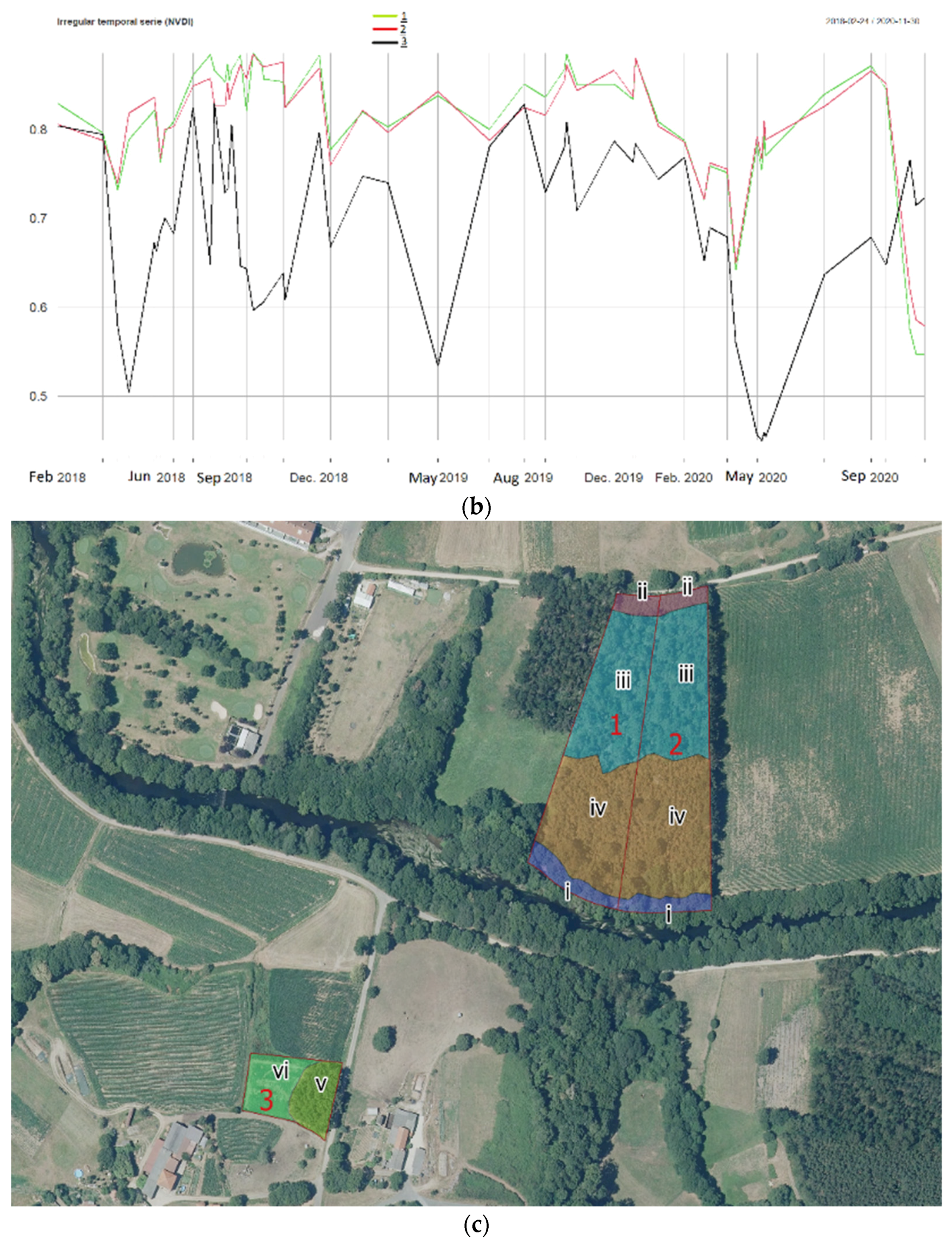
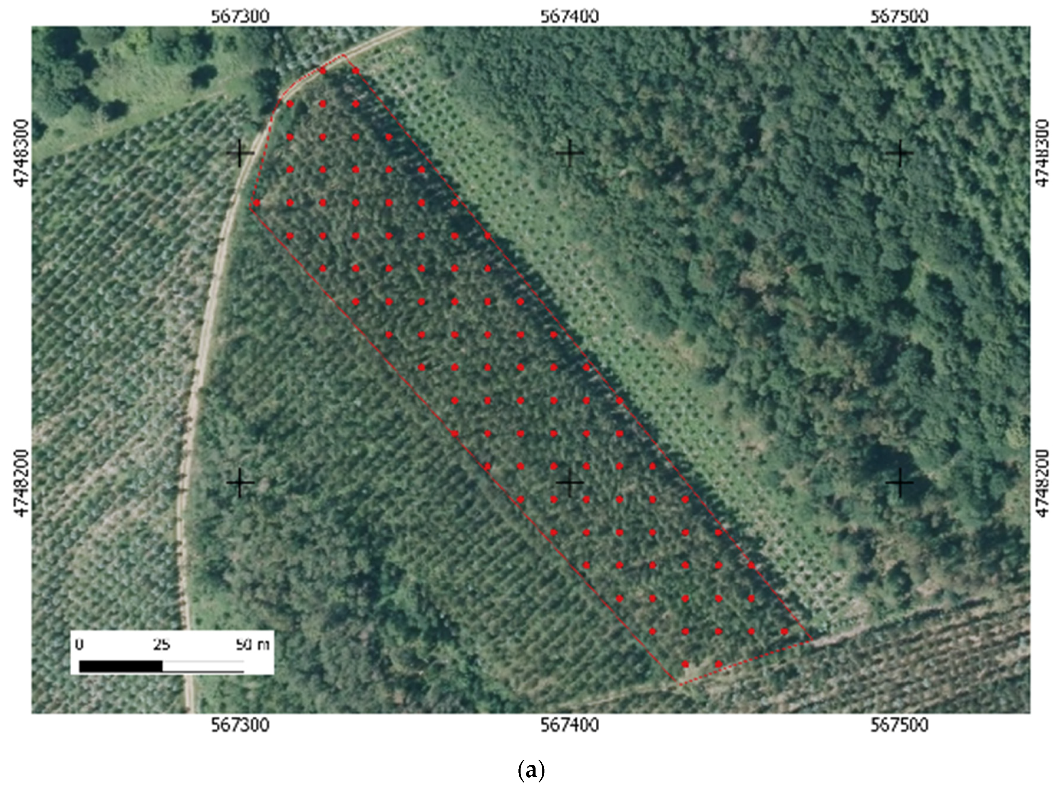
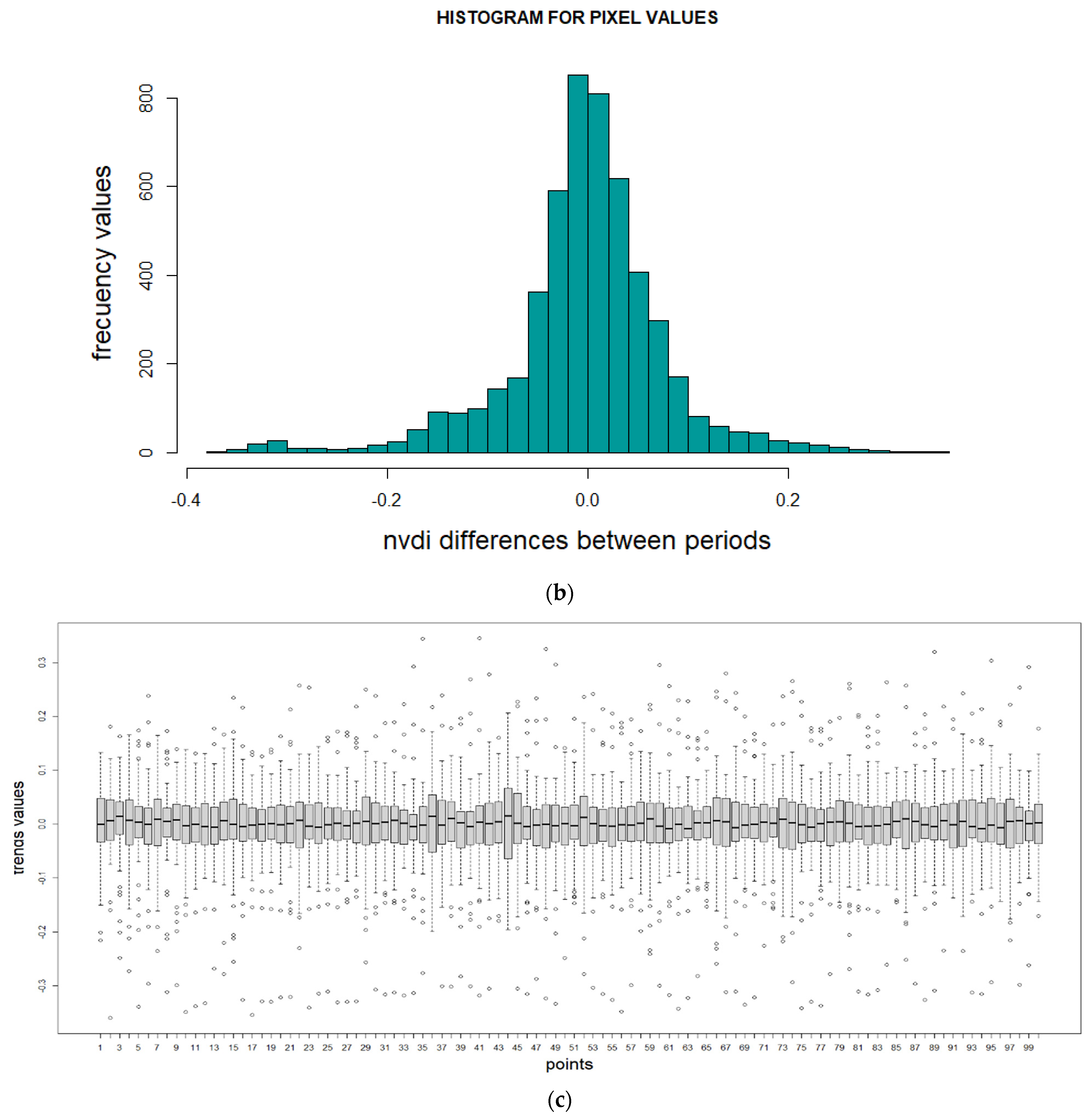
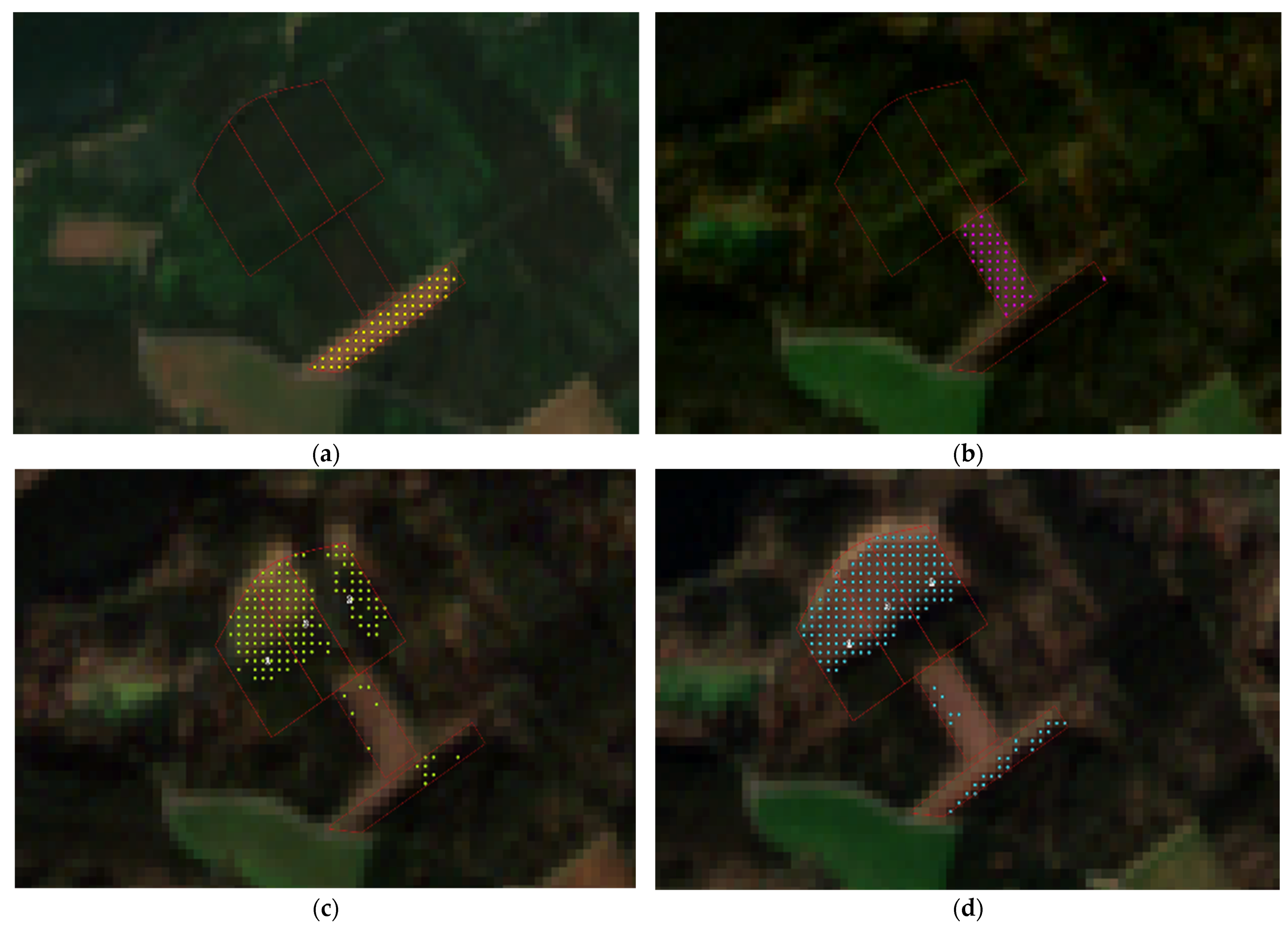
| 2018 | 2019 | 2020 |
|---|---|---|
| 24/02/2018 | 14/02/2019 | 24/02/2020 |
| No data | 16/03/2019 | 18/03/2020 25/03/2020 |
| 18/04/2018 | No data | 14/04/2020 24/04/2020 |
| 05/05/2018 18/05/2018 | 13/05/2019 | 19/05/2020 24/05/2020 27/05/2020 29/05/2020 |
| 17/06/2018 19/06/2018 24/06/2018 | No data | No data |
| 09/07/2018 | 12/07/2019 | No data |
| 01/08/2018 21/08/2018 26/08/2018 | 21/08/2019 | 05/08/2020 |
| 07/9/2018 | 15/09/2019 | 29/09/2020 |
| 10/09/2018 10/10/2018 20/10/2018 22/10/2018 | 07/10/2019 10/10/2019 22/10/2019 | 16/10/2020 |
| 14/11/2018 | No data | 13/11/2020 20/11/2020 30/11/2020 |
| 26/12/2018 | 04/12/2019 26/12/2019 | No data |
| Accuracy | TP = true positive, TN = true negative, FP = false positive, FN = false negative | |
| 95% CI | = the sample mean = margin of error N = standard error | |
| p-value (ACC < NIR) | = the sample proportion p0 = the hypothesized proportion n = the sample size ACC = accuracy NIR = No information rate p-value for ACC > NIR | |
| Kappa | P0 = proportion of trials in which judges agree Pe = proportion of trials in which agreement would be expected due to chance | |
| Mcnemar’s Test | - | |
| Sensitivity | TP = true positive, FN = false negative | |
| Specificity | TN = true negative, FP = false positive | |
| Pos. Pred Value | ×100 | TP = true positive, FP = false positive |
| Neg. Pred Value | ×100 | TN = true negative, FN = false negative |
| Prevalence | I = incidence, D = duration | |
| Detection Rete | TP = true positive, FP = false positive | |
| Detection Prevalence | - | |
| Balanced Accuracy | - |
| Confusion Matrix and Statistics | |
|---|---|
| Accuracy | 0.8862 |
| 95% CI | (0.8164, 0.9364) |
| No Information Rate | 0.7236 |
| p-value (ACC < NIR) | 1.044 × 10⁻⁵ |
| Kappa | 0.7047 |
| Mcnemar’s Test | 0.4227 |
| Sensitivity | 0.7353 |
| Specificity | 0.9438 |
| Pos. Pred Value | 0.8333 |
| Neg. Pred Value | 0.9032 |
| Prevalence | 0.2764 |
| Detection Rete | 0.2033 |
| Detection Prevalence | 0.2439 |
| Balanced Accuracy | 0.8396 |
Publisher’s Note: MDPI stays neutral with regard to jurisdictional claims in published maps and institutional affiliations. |
© 2021 by the authors. Licensee MDPI, Basel, Switzerland. This article is an open access article distributed under the terms and conditions of the Creative Commons Attribution (CC BY) license (https://creativecommons.org/licenses/by/4.0/).
Share and Cite
López-Amoedo, A.; Álvarez, X.; Lorenzo, H.; Rodríguez, J.L. Multi-Temporal Sentinel-2 Data Analysis for Smallholding Forest Cut Control. Remote Sens. 2021, 13, 2983. https://doi.org/10.3390/rs13152983
López-Amoedo A, Álvarez X, Lorenzo H, Rodríguez JL. Multi-Temporal Sentinel-2 Data Analysis for Smallholding Forest Cut Control. Remote Sensing. 2021; 13(15):2983. https://doi.org/10.3390/rs13152983
Chicago/Turabian StyleLópez-Amoedo, Alberto, Xana Álvarez, Henrique Lorenzo, and Juan Luis Rodríguez. 2021. "Multi-Temporal Sentinel-2 Data Analysis for Smallholding Forest Cut Control" Remote Sensing 13, no. 15: 2983. https://doi.org/10.3390/rs13152983
APA StyleLópez-Amoedo, A., Álvarez, X., Lorenzo, H., & Rodríguez, J. L. (2021). Multi-Temporal Sentinel-2 Data Analysis for Smallholding Forest Cut Control. Remote Sensing, 13(15), 2983. https://doi.org/10.3390/rs13152983


