Abstract
Hydro-climatic resilience is an essential element of food security. The miombo ecosystem in Southern Africa supports varied land uses for a growing population. Albedo, Leaf Area Index (LAI), Fractional Vegetation Cover (FVC), Solar-Induced chlorophyll Fluorescence (SIF), and precipitation remote-sensing data for current climate were jointly analyzed to explore vegetation dynamics and water availability feedbacks. Changes in the surface energy balance tied to vegetation status were examined in the light of an hourly albedo product with improved atmospheric correction derived for this study. Phase-space analysis shows that the albedo’s seasonality tracks the landscape-scale functional stability of miombo and woody savanna with respect to precipitation variations. Miombo exhibits the best adaptive traits to water stress which highlights synergies among root-system water uptake capacity, vegetation architecture, and landscape hydro-geomorphology. This explains why efforts to conserve the spatial structure of the miombo forest in sustainable farming of seasonal wetlands have led to significant crop yield increases. Grass savanna’s high vulnerability to water stress is illustrative of potential run-away impacts of miombo deforestation. This study suggests that phase-space analysis of albedo, SIF, and FVC can be used as operational diagnostics of ecosystem health.
1. Introduction
Global warming due to anthropogenic causes such as greenhouse gas emissions impacts the interconnected climate, hydrological, environmental/ecological, and social systems, that is the Earth system [1,2]. Land-use and land cover dynamics are crucial for modeling climate change impacts, particularly in areas with intensive agricultural practices and population growth. Agricultural lands cover approximately 40% of the land surface of the Earth, and population increases worldwide present challenges for sustainable food production and water resource management [3,4]. One of the main issues hindering African development is drought, making up fewer than 20% of natural disasters in Sub-Saharan Africa but more than 80% of the population affected by natural disasters in this region [5,6]. For example, drought can intensify in dry areas resulting from increased evaporation and enhanced atmospheric moisture holding capacity caused by warming [1]. Projected increases in water scarcity in combination with restricted access to groundwater can in turn lead to increased risk of heat waves and wildfires with devastating impacts on African communities dependent on rainwater as a primary water source [1,2,7,8,9].
In Southern Africa, rainfed agriculture dominates 95% of the agricultural sector, leaving the region particularly susceptible to precipitation changes resulting from a warming climate [5,10,11,12,13]. Among many other climate hazard impacts, agricultural yields have been influenced by natural land cover change, drought, fires, altered crop nutrient content, plant infections, and more [1,14,15,16]. Regional projections in Southern Africa estimate a 15% to 50% decrease in agricultural productivity from climate change [10]. The miombo ecosystem, located in the transition area from the rainforests near the equator to the semi-arid woodlands of Southern Africa, supports commercial farming, wildlife conservation, tourism, and small-scale agriculture that tens of millions of people rely on. These diverse land uses, along with the wide areal extent and prevalence of woodlands throughout the miombo, give the region significant potential as either a global carbon source or a sink, which is contingent upon how land-use management strategies are implemented [17,18,19,20,21]. In south central Africa, human populations are growing faster than the supporting economy [18]. Coupled with a lack of resources for agricultural intensification in the region, croplands are expanding to accommodate the increase in food demand, mostly at the expense of existing miombo woodlands [18,22]. Previous studies show that, with management strategies such as community-based forest management [23,24], improvements in miombo density and biomass hold potential as mitigation strategies for climate change. However, the long-term interactions between land-use/land cover and climate change in this ecosystem are not well quantified due to their complex, nonlinear nature and modeling uncertainties, as well as a lack of studies assessing vegetation change over long periods of time [17,25,26]. While many studies focus on greenhouse gas emissions in describing climate impacts on the miombo ecosystem, biophysical impacts, such as the link among rain, radiative forcing, and vegetation should also be further investigated [21,27,28]. As such, a dynamic systems approach focusing on the underlying processes of land–atmosphere interactions in the miombo needs to be developed [17].
Models of future precipitation and agricultural productivity rely heavily on moisture and heat exchange between the atmosphere and land surface. In water-limited ecosystems with discontinuous distributions of vegetation [29,30,31,32], soil moisture integrates the effects of vegetation, soil, and climate on the dynamics. Previous studies suggest a positive feedback between vegetation and soil moisture, since subcanopy soils are often moister than patches between canopies [32,33,34,35,36,37,38,39,40,41]. In terms of surface energy fluxes, the portion of total solar radiation that is reflected by Earth’s surface, or surface albedo, is a critical parameter for determining radiative energy fluxes on land. Decreased albedo generally corresponds to increased vegetation, which tends to be darker than bare soil [42]. Persistent increases in albedo in natural systems in the tropics are associated with decreases in vegetation cover [42,43,44]. Decreases in vegetation cover result in decreases in evapotranspiration and decreases in near surface soil moisture due to loss of canopy shade as well as inhibition of biophysical pumping of deep water by active root systems. In areas with dense vegetation, over 70% of average net radiation is transferred to latent heat flux, while under 30% is converted to sensible heat flux [44]. In dry areas with bare soil, evaporation rates are very low, so a large portion of net radiation is converted to sensible heat flux. This in turn leads to decreases in moist static energy in the planetary boundary layer (PBL) and suppression of moist convection (e.g., [44,45,46]). Spatial and temporal variability of radiative properties such as surface albedo (∼20%) and emissivity (∼2%) have significant impacts on the diurnal cycle of the land-surface energy budget with up to 10–20% changes in sensible and latent heat fluxes [47].
Since albedo calculations present a major radiative uncertainty in climate modeling, high-resolution remotely sensed aerosol optical depths and Ross-Thick Li-Sparse Reciprocal (RTLS) kernel parameters were obtained to estimate the albedo at the surface. These data were developed with the Multi-Angle Implementation of Atmospheric Correction (MAIAC) algorithm, which uses the time series of measurements from the Moderate Resolution Imaging Spectroradiometer (MODIS) to collect aerosol optical thickness and surface Bi-directional Reflectance Distribution Function (BRDF) retrievals simultaneously [48,49]. Along with MODIS land surface temperature data, Global 30 Arc-Second Elevation (GTOPO30) digital elevation data, Famine Early Warning Systems Network (FEWS NET) Land Data Assimilation System (FLDAS) surface pressure products, aerosol optical depths, and RTLS kernel parameters were used to calculate hourly spectral narrowband and shortwave broadband albedo datasets over the span of 10 years (2009–2018).
In addition to estimating albedo to improve radiative uncertainty and examine surface energy changes, vegetation parameters were retrieved to map plant dynamics in response to different hydrometeorological conditions from year to year. Data such as the Leaf Area Index (LAI) and Fractional Vegetation Cover (FVC) facilitate the tracking and evaluation of changes in the biophysical properties and photosynthetic rates of canopy and other plant cover [50,51]. LAI and FVC are based on remotely sensed spectral signatures, and Solar-Induced chlorophyll Fluorescence (SIF) provides a more direct approach for predicting changes in photosynthetic efficiency that are not easily detected by changes in reflectance [51]. Depending on canopy condition that is measured by LAI, increases in vegetation cover increase shade effectively leading to lower temperatures near the ground. Phase-space analyses were conducted with albedo, SIF, LAI, and FVC to understand the vegetation life cycle and diurnal land–atmosphere dynamics of the miombo ecosystem. Joint, spatial analyses of these multi-sensor data with precipitation at different nominal spatial resolutions enabled intercomparisons to examine the consistency of the representation of spatial heterogeneity across the different sensors.
The main objectives of this study were: (1) to illustrate the utility of remote sensing data for capturing feedbacks between precipitation variations, vegetation dynamics, and water availability; (2) to provide a quantitative understanding of natural ecosystem resilience in the region to water stress and changes in climate and its potential agricultural applications through remotely-sensed land surface monitoring. Section 2 covers the materials and methods, namely the study area’s topography and climatology and data processing methodology for precipitation data, vegetation parameters, land cover mapping, albedo, SIF analysis, and joint data analyses. Section 3 covers the main results and discussion regarding the spatiotemporal variability of rainfall, spatial variability of vegetation data, SIF analysis, spatiotemporal variability of albedo, phase-space analysis, seasonal and interannual variability of albedo and vegetation, data anomalies, uncertainty, and future directions. Section 4 contains the main conclusions regarding the interactions among rainfall variability, soil moisture availability, and root water uptake demonstrated by analysis of remotely sensed land-surface properties and the functional behaviors of different land cover types as illustrated by phase-space analysis. The interplay between the hydrologic behavior of dambos (e.g., seasonal wetlands in the headwaters) and the miombo trees is further discussed in the light of potential implications for long-term, sustainable agriculture.
2. Materials and Methods
2.1. Study Area
The Upper Zambezi River Basin’s (UZRB) ecosystem consists of miombo, tree savanna, grasslands, and wetlands in an arid to semi-arid transition zone between the Kalahari Desert to the south and the tropical rainforest of the Congo to the north [52]. Figure 1 shows a digital elevation map of the UZRB. In arid ecosystems, productivity is driven primarily by soil water content, and the seasonal cycle of productivity is driven by soil moisture in larger part than by vapor pressure deficit [53]. The climate of this area is characterized by complex rainfall gradients driven by the movement of the Inter-Tropical Convergence Zone (ITCZ), a narrow, clearly defined band of clouds that stretches around the globe parallel to the equator [54,55]. The ITCZ moves northward during the cooler, dry season (May to October), generating an average accumulated precipitation of less than 100 mm. During the warmer, rainy season (November to April), the ITCZ moves southward, resulting in an average accumulated precipitation between 700–1000 mm [52] (see Table S1 in the Supplementary Materials for average accumulated seasonal rainfall values).
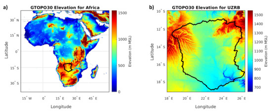
Figure 1.
Digital elevation map of (a) Africa and (b) the Upper Zambezi River Basin (UZRB) with the UZRB outlined in black. MSL, Mean Sea Level. Note the different elevation scales on the left (0 to 1550 m MSL) and on the right (650 to 1550 m MSL).
2.2. Data, Processing, and Calculations
Table 1 summarizes the data products used for this project. The UZRB spans two tiles in sinusoidal projection used in the canonical MODIS products. All MODIS data used in this study were stitched and re-projected to UTM 34S projection using the HDF-EOS to GeoTIFF (HEG) Conversion Tool [56]. Since the ITCZ over this region often results in cloud-contaminated pixels, a software package called TIMESAT performed adaptive temporal filtering using the Savitzky–Golay method to smooth out anomalies and discontinuities in the data impacted by cloud contamination [57]. This is accomplished by using time series data, quality control information, and moving windows to fit a quadratic polynomial function. All data products were re-scaled and re-projected to 1 km, UTM 34S projection with various methods depending on the underlying physics and original spatial resolution of each product described in the following sections.

Table 1.
Summary of data products.
2.2.1. Precipitation Data
Integrated Multi-satellitE Retrievals for Global Precipitation Measurement (IMERG) precipitation intensity data at 0.1° (∼10 km), monthly resolution were obtained from the National Aeronautics and Space Administration (NASA) Precipitation Processing System’s (PPS) Science Team On-Line Request Module (STORM) [70]. The original data were bilinearly interpolated to 1 km spatial resolution. Accumulated precipitation data were calculated by multiplying the monthly mean precipitation intensities by the time period of interest (i.e., converted from mm/h to mm/month, mm/season, mm/period, or mm/year).
2.2.2. Vegetation Data
MODIS MCD15A3H Version 6 Leaf Area Index (LAI) products at 4-day, 500 m resolution were re-projected with the HEG tool, cloud-corrected in TIMESAT (Figure 2), and aggregated to 1 km spatial resolution by taking the average of every four pixels with a final 4-day, 1 km resolution [65]. LAI is representative of canopy cover, which is linked to surface energy balance and modulates interactions between vegetation, hydrologic processes, and the atmosphere, such as evapotranspiration, rainfall interception, throughfall, and stemflow [73,74].
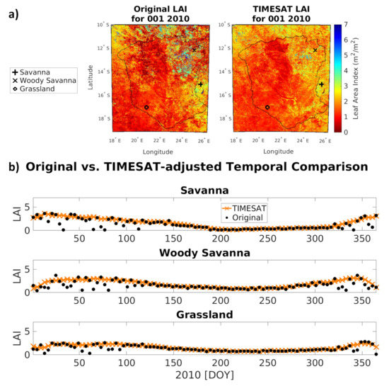
Figure 2.
(a) Spatial and (b) temporal comparisons between 2010 original and new TIMESAT-corrected Leaf Area Index (LAI) data.
Global ’Orbiting Carbon Observatory-2 (OCO-2)’ solar-induced chlorophyll fluorescence (GOSIF) data were obtained from the Global Ecology Group’s Data Repository at 8-day, 0.05° resolution and OCO-2 SIF data were obtained from the Goddard Earth Sciences Data and Information Services Center (GES DISC) at 16-day, 2.25 km by 1.29 km resolution [68,69]. For the purposes of this manuscript, SIF and GOSIF are used interchangeably unless otherwise specified (i.e., OCO-2 SIF used in SIF analysis is a separate data product from GOSIF). This fluorescence is emitted directly from the core of photosynthetic machinery and is thus indicative of vegetative photosynthetic status, unlike other vegetation indices that describe “greenness” [68]. SIF can serve as a proxy for ecosystem gross primary productivity (GPP), with strong correlations between SIF and GPP climatologies on the monthly scale for deciduous broadleaf, mixed forest, evergreen needleleaf forests, and croplands [53]. Significant correlations with higher variability have been observed for land cover types including savanna, evergreen broadleaf, and shrublands [53]. SIF data were re-projected in the Quantum Geographic Information System (QGIS) to UTM 34S projection, and then interpolated using nearest-neighbor to 1 km spatial resolution. OCO-2 SIF are kept at the original resolution, and comparisons between the two data are made by selecting GOSIF values that are closest geographically to each OCO-2 orbit overpass.
Fractional Vegetation Cover (FVC) was calculated using a semi-empirical method (Equation (1)) based on the Normalized Difference Vegetation Index (NDVI) (Equation (2)) [75]. NDVI is a measure of “greenness” that exploits chlorophyll reflectance of near-infrared light and absorption of visible red light [76]. Any FVC values over 1 were set to 1, and any pixels whose LAI values were 3 or higher were also assumed to have 100% FVC.
where is the NDVI corresponding to bare soil () and is the NDVI corresponding to full vegetation cover (), which were approximated after systematic inspection of MODIS NDVI time series graphs. is the time-varying NDVI value calculated from TIMESAT-corrected MODIS MCD43A4 Version 6 Band 1 () and Band 2 () reflectance data that was aggregated by taking the average of every four 500 m pixels to 1 km resolution with daily time steps [76], given by:
2.2.3. Land Cover Re-Classification
The MODIS MCD12Q1 Version 6 product’s International Geosphere-Biosphere Programme (IGBP) land cover classification system was used to characterize land cover in the UZRB [58]. The data were downloaded at annual, 500 m spatial resolution and aggregated by taking the mode of every four pixels to 1 km resolution, then re-classified into six main land cover types: miombo, tree savanna, grass savanna, wetland, water, and barren/built-up. The re-classification is presented in Table 2. Larger trees and shrublands in the IGBP classification were assumed to be representative of miombo because the understory in miombo woodlands is scattered and composed of suppressed tree saplings and broadleaved shrubs [18,77]. Sedges, forbs, and grasses sparsely but continuously cover the ground layer [18,77]. The dominant tree species in miombo are of the genera Brachystegia, Julbernardia, and/or Isoberlinia, which are unique to miombo ecosystems [18,77,78,79]. Other important species include Burkea africana, Pseudolachnostylis maprouneifolia, Diplorhynchus condilocarpon, and more [18,77]. The large broadleaf trees are characteristic of wet miombo, where canopy cover is dense and trees are over 15 m in height [18,77]. In the IGBP classification, open and closed shrublands contain woody perennials 1–2 m in height, which is characteristic of Eriosema, Sphenostylis, Kotschya, Dolichos, and Indigofera perennial plants that dominate the shrub composition of dry miombo [18]. Since the IGBP classification provides woody savanna, savanna, grassland, and cropland land cover classes that are distinct from shrubland land cover, the IGBP classes were assumed to cover all woody savanna and grass savanna land cover types. The same re-classification was used by Lowman et al. (2018) [52] to represent Southern Africa using MCD12Q1 Version 5 data instead of MCD12Q1 Version 6 data.
Table 2.
Land cover classes.
Using the same methodology as Lowman et al. (2018) [52], dynamic wetland maps were created using five wetland predictor variables derived from MODIS MCD43A4 Version 6 Nadir BRDF-adjusted reflectance data after aggregation to 1 km resolution with daily temporal resolution [59,60]. These indices aid in visualizing seasonal changes in wetland area, and stationary land cover data for three consecutive wet years (2010–2012) were used as training data for wetland probability mapping (Appendix A) considering six wetland indices (Figure 3c–h). Two distinct peaks in the histograms generally signifies a “good” wetland predictor. As such, NDVI, which has the greatest amount of overlap between wetland and non-wetland values and the most irregular peaks, was not used as a wetland predictor variable. As shown in Figure 3b, threshold area curves were generated for 2009 to 2018, indicating that, at scales above 150 km, there is less uncertainty with wetland mapping. At finer resolutions, uncertainty increases greatly and varies according to interannual variability in climate and weather. For example, a 60% threshold yields uncertainty on the order of 100%. Based on the black line in Figure 3b marking the permanent wetland area derived from stationary land cover between 2010 and 2012 (Figure 3a), a threshold value of 99% was selected. Compared to previous work on wetland probability mapping [52] that used MCD12Q1 Version 5 data processed with the now-retired MODIS Reprojection Tool (MRT), the MCD12Q1 Version 6 data processed with the HDF-EOS to GeoTIFF Conversion Tool refines the permanent wetland class in the stationary land cover and thus highlights the interannual variability in wetland extent tied to precipitation. These dynamic wetland area maps were overlaid onto the land cover maps to complete the reclassification, as shown in Figure 4.
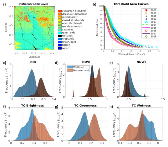
Figure 3.
(a) Stationary land cover map based on Moderate Resolution Imaging Spectroradiometer (MODIS) MCD12Q1 Version 6 data for three wet years (2010–2012), along with (b) threshold-area curves for 2009–2018. The black line indicates the permanent wetland area of the stationary land cover map. (c–h) Histograms of wetland and non-wetland pixels from training data using: (c) Near-Infrared Reflectance (NIR) data; (d) the Normalized Difference Vegetation Index (NDVI); (e) the Normalized Difference Water Index (NDWI); (f) Tasseled Cap (TC) Brightness; (g) TC Greenness; (h) TC Wetness.
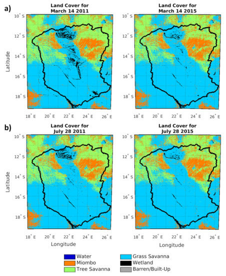
Figure 4.
Seasonal land cover derived from MODIS MCD12Q1 land cover classes for a wet year (2011; left) and a dry year (2015; right) to compare (a) wetland extent after the peak of the rainy season to (b) wetland extent during the middle of the dry season.
Figure 5 displays varying vegetation densities of the three land cover types of interest in this study: grass savanna, miombo, and woody savanna. Miombo trees are generally taller and more densely packed, with extensive root systems that can reach up to 27 m in lateral length and over 5 m in vertical depth [17]. On the other hand, woody savanna trees are shorter and more spread out, with smaller root systems ranging 2–12 m laterally and 0.7–1.5 m vertically [80]. Grass savanna vegetation are the least dense with shallow root systems, often containing seasonally waterlogged wetland areas and shallow depressions called dambos that intersperse the landscape [17]. Figure 6 illustrates relative sizes and root zone distributions of woody savanna, grass savanna, and miombo.
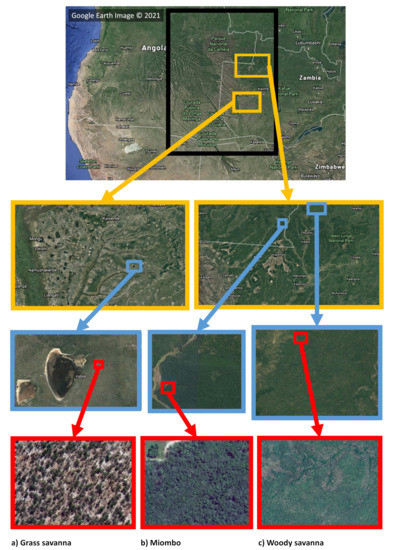
Figure 5.
Google Earth images comparing vegetation densities of three different land cover types in the UZRB: (a) grass savanna; (b) miombo; (c) woody savanna [81]. Google Earth Image ©2021: Google, Data SIO, National Oceanic and Atmospheric Administration (NOAA), U.S. Navy, National Geospatial-Intelligence Agency (NGA), General Bathymetric Chart of the Oceans (GEBCO), Landsat/Copernicus, AfriGIS (Pty) Ltd, International Bathymetric Chart of the Arctic Ocean (IBCAO), Maxar Technologies, Centre National D’Etudes Spatiales (CNES; National Centre for Space Studies)/Airbus.
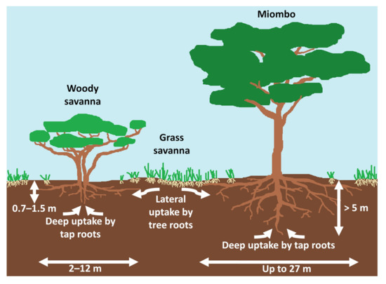
Figure 6.
Diagram depicting varying spatial distributions of root zones for woody savanna, grass savanna, and miombo land cover types. The diagram was not drawn to scale, but approximate sizing was determined based on tree heights, vertical root depths, and lateral root lengths found in the literature [17,80].
2.2.4. Albedo Algorithm
Given the lack of hourly albedo data available for this region, surface albedo data were derived from MODIS MAIAC MCD19A2 aerosol optical depth (AOD) and MCD19A3 bi-directional reflectance distribution function (BRDF) model parameter data using existing methodology [61,62,82]. Figure 7 depicts the surface albedo data processing and calculations flowchart with final spatial and temporal resolutions specified for each data product.
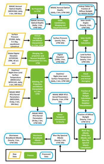
Figure 7.
Surface albedo data processing and calculations flowchart. MAIAC, Multi-Angle Implementation of Atmospheric Correction. SIN, MODIS SINusoidal projection. UTM, Universal Transverse Mercator projection. FLDAS, Famine Early Warning Systems NETwork (FEWS NET) Land Data Assimilation System. GTOPO30, Global 30-Arc Second Elevation. BRDF, Bi-directional Reflectance Distribution Function. RTLS, Ross-Thick Li-Sparse.
Black-Sky Albedo (BSA), or directional-hemispherical reflectance, is the albedo of a surface illuminated in one direction. Equation (3) describes how BSA is calculated by a simplified polynomial expression to represent the integration of the BRDF over the exitance hemisphere for a single irradiance direction [83]. White-Sky Albedo (WSA), or bi-hemispherical reflectance, is the surface albedo generated by diffuse illumination. Equation (4) describes how WSA is calculated by a simplified polynomial expression to represent the integration of the BRDF over all viewing and irradiance directions [83]. Famine Early Warning Systems Network (FEWS NET) Land Data Assimilation System (FLDAS) surface pressure, Global 30 Arc-Second Elevation (GTOPO30) digital elevation, and MODIS MOD11A1/MYD11A1 land surface temperature data were inputted into the National Renewable Energy Laboratory’s Solar Position Algorithm (NREL SPA) to calculate the hourly solar zenith angles (SZA) for each pixel [63,64,66,67,84].
where is black-sky albedo, is white-sky albedo, is the solar zenith angle, is the wave band, are the Ross-Thick Li-Sparse (RTLS) kernel parameters (), and , , and are the coefficients corresponding to each RTLS parameter presented in Table 3.
Table 3.
Black-sky albedo coefficients from [85].
To obtain fraction of diffuse skylight (SKYL) values, a look-up table retrieved from the MODIS User Tools section of Professor Crystal Schaaf’s Lab site was used to bilinearly interpolate SKYL values based on AOD and SZA values [86]. These SKYL values act as weights for calculating blue-sky albedo, or albedo corresponding to actual atmospheric conditions, from an interpolation between BSA and WSA, as shown in Equation (5) [83]:
where is narrowband blue-sky albedo, is the fraction of diffuse skylight, and is the aerosol optical depth. The seven resulting narrowband blue-sky albedos were then combined to calculate shortwave broadband albedo using Equation (6) [83]:
where is the broadband albedo and is the conversion coefficient corresponding to MODIS reflectance band i presented in Table 4.
Table 4.
Narrowband spectral-to-broadband albedo conversion coefficients from [48,85].
2.2.5. Orbit-Based SIF Analysis
Since GOSIF data were derived from MODIS data, Modern-Era Retrospective Analysis for Research and Applications, Version 2 (MERRA-2) meteorological reanalysis data, and OCO2-SIF data, both GOSIF and OCO-2 SIF datasets were compared in an orbit-based analysis. GOSIF data were corrected with a 24 h daily correction factor, while OCO-2 SIF data were corrected with the following daytime-only daily correction factor (any SZAs over 90° were set to 90°) in Equation (7) [87]:
where is the average daily SIF value, is the instantaneous OCO-2 SIF value at 757 nm, is the beginning time (sunrise for daytime-only), is the end time (sunset for daytime-only), is the instantaneous solar zenith angle at the time the observation was taken, , and is the solar zenith angle at time t. To match the 24 h daily correction factor calculations provided in the OCO-2 User Guide as closely as possible, the solar zenith angles were calculated at 10-minute intervals using the NREL SPA, and the integral was approximated via the trapezoidal method for daytime hours only [84,87]. Only OCO-2 SIF observations collected under nadir and for clear skies conditions were used, since the Cubist regression tree model used to produce GOSIF from OCO-2 soundings averaged OCO-2 SIF data collected under similar conditions [68].
2.2.6. Data Analysis
For each year of interest (e.g., 2010–2011 and 2015–2016), the data were compared in phase-space plots by masking the data for each land cover type and calculating the mean values and 95% confidence intervals over time. Ellipses were then overlaid onto the graphs to approximate the shape of the limit-cycles with arrows to indicate the direction of time. The time period for each graph was not based off of the calendar year so that the data points would represent two consecutive rainy and dry seasons.
To explain anomalous seasonality in the albedo data, the slope of the terrain was examined using GTOPO30 digital elevation data in QGIS to determine where flat land or water may impact the data values. When other anomalous behavior was identified in specific locations in the landscape, phase-space graphs for albedo and fractional vegetation cover were plotted as well.
3. Results and Discussion
3.1. Spatial and Temporal Variability of Precipitation
Spatial and bar graph comparisons of mean monthly accumulated precipitation are displayed in Figure 8 and Figure 9, respectively.
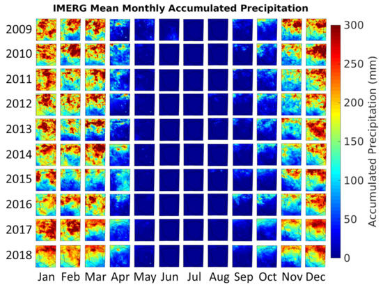
Figure 8.
Spatial comparisons of Integrated Multi-satellitE Retrievals for Global Precipitation Measurement (IMERG) mean monthly accumulated precipitation for 2009–2018.

Figure 9.
Bar graph comparisons of IMERG mean monthly accumulated precipitation for 2009–2018 for all land cover, miombo, grass savanna, and woody savanna.
In general, 2009–2014 and 2017–2018 were relatively wet years, while 2015 and 2016 were relatively dry years (see Table S1 in the Supplementary Materials). Based on the spatial interannual comparisons (Figure 8) and land cover comparisons (Figure 9), the northern areas of the basin where miombo and woody savanna dominate receive more accumulated rainfall on average than the southern portion where grass savanna dominates.
3.2. Spatial Variability of Vegetation
Seasonal spatial comparisons of LAI, SIF, and FVC are displayed in Figure 10. The use of an NDVI-based fractional vegetation cover calculation appears to highlight the flush of grasses during the rainy season and their subsequent senescence during the dry season characteristic of semi-arid regions in Africa [88]. Woody savanna and miombo retain some fractional vegetation cover during the dry season, which could be attributed to frequent accidental and deliberate fires as people prepare land for harvest or for livestock grazing. The miombo ecosystem likely contains the largest burned area globally estimated at approximately 1 million km yr [17]. These fires generally decimate grasses, shrubs, and fine woody biomass, but trees and other woody plants often persist, re-sprouting quickly from any remaining root systems and stems [17]. LAI and SIF data reflect similar seasonal contrasts, although the tree savanna LAI data in the northwest portion of the UZRB appear to be less sensitive across both seasons. This could be attributed to the smoothing effect of the TIMESAT cloud correction since many pixels were cloud-contaminated during the peak of the rainy season demonstrated by the large fluctuations in original LAI values, particularly for the woody savanna pixel shown in Figure 2. In addition, the seasonally inundated grass savanna/wetland areas in the center of the basin consistently have low values of LAI, GOSIF, and FVC that are distinct from the seasonal greening and senescence observed in other grass savanna areas in the southern portion of the basin. The wetland areas mapped in Figure 4 are based on a 99% threshold from the wetland probability maps determined using stationary MODIS MCD12Q1 permanent wetland pixels (Figure 3b), but the actual wetland areal extent may cover a larger, sparsely vegetated area marked by the low (red) values in Figure 10 that the MODIS (LAI and FVC) and OCO-2/MERRA-2 instruments (GOSIF) are able to detect.
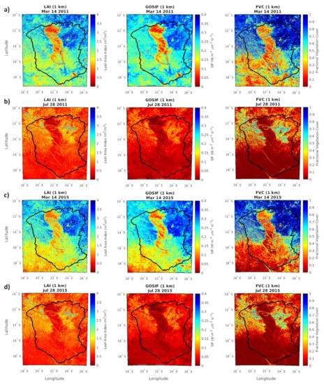
Figure 10.
Spatial comparisons of (a,b) 2011 and (c,d) 2015 Leaf Area Index (LAI), Solar-Induced chlorophyll Fluorescence (SIF), and Fractional Vegetation Cover (FVC) (a,c) just after the peak of the rainy season and (b,d) during the middle of the dry season.
Orbit-Based SIF Analysis
The results of the orbit-based SIF analysis in Figure 11a,c display GOSIF values that are more densely concentrated between 0 and 0.4 W mm sr, while the OCO-2 SIF values are more variable over a wider range of SIF values. Despite the many advantages of GOSIF in its global, continuous coverage and longer record (2000–2020), these results suggest that the application of the daily correction factor over 24 h may be underestimating the SIF signal because nighttime values were taken into account. On the other hand, the GOSIF data appear to capture seasonal trends more clearly (Figure 11a), with values ranging around 0.15–0.4 W mm sr during the rainy season and around 0–0.2 W mm sr during the dry season (Figure 11b).
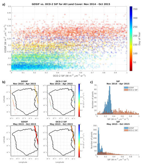
Figure 11.
Global ’OCO-2’ Solar-Induced chlorophyll Fluorescence (GOSIF) vs. Orbiting Carbon Observatory-2 (OCO-2) orbit-based comparisons. (a) Cloud bias plot depicting pixels for all land cover types between 2014–2015. (b) Spatial comparisons of GOSIF and OCO-2 orbits and (c) histogram comparisons of the distribution of nadir-only, clear skies SIF observations. OCO-2 data here are corrected with a daytime-only daily correction factor, while GOSIF data are corrected with a 24 h daily correction factor.
3.3. Spatial and Temporal Variability of Shortwave Broadband Albedo
Figure 12 shows an example of 2011 BSA, WSA, and actual blue-sky spectral albedo values at noon local time for MODIS Band 2 (near-infrared) during the rainy season (Figure 12a) and the dry season (Figure 12b). Figure 13 depicts spatial graphs of 2011 (Figure 13a,b) and 2015 (Figure 13c,d) shortwave broadband albedo for times after sunrise, at noon, and before sunset local time. Figure 14a displays time series comparisons of 2009 to 2018 monthly mean diurnal cycles of surface albedo for three different land cover types along with land cover values (Figure 14b) and albedo values (Figure 14c) for reference. The locations of the three pixels within the basin used for the interannual monthly mean diurnal cycle comparison (Figure 14a) for each land cover type are marked in Figure 14c with a black plus sign for miombo, a black cross for tree savanna, and a black circle for grass savanna. Figure 14d displays the annual (calendar year) mean accumulated precipitation values across the basin for each year from 2009 to 2018.
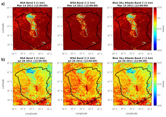
Figure 12.
Example of Black-Sky Albedo (BSA), White-Sky Albedo (WSA), and blue-sky spectral albedo comparisons between dates in (a) the rainy season (14 March 2011) and (b) the dry season (28 July 2011) at noon local time.
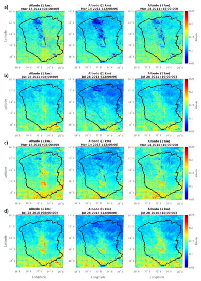
Figure 13.
Spatial comparisons of (a,b) 2011 and (c,d) 2015 shortwave broadband albedo for morning, noon, and afternoon local times (a,c) just after the peak of the rainy season and (b,d) during the middle of the dry season.
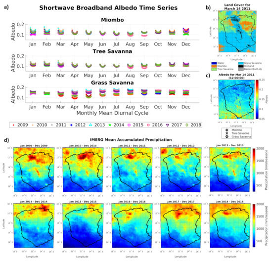
Figure 14.
(a) Time series comparison of 2009–2018 monthly average diurnal cycles of shortwave broadband albedo for three different land cover types. The 2011 rainy season (b) land cover and (c) shortwave broadband examples with the miombo (plus sign), tree savanna (cross), and grass savanna (circle) pixels corresponding to the time series marked spatially with black symbols. (d) IMERG precipitation data for each calendar year between 2009 and 2018.
Based on these results, the hourly shortwave broadband albedo exhibits a diurnal cycle expected of actual albedo because of the data’s dependence on instantaneous solar zenith angles. The spatial graphs (Figure 13) suggest that albedo values are generally under 0.12 for inundated areas in the wetlands during the rainy season around noon local time (see Table S2 for mean annual albedo values corresponding to permanent wetlands). Surface albedo was also consistent with land cover differences during peak sunlight hours (i.e., noon local time), which makes sense given that the solar zenith angle and subsequently the fraction of diffuse skylight at those times is smaller. Assuming albedo estimates at noon local time are representative of actual albedo, increases in solar zenith angle (i.e., after sunrise and before sunset in Figure 12 and Figure 13) appear to overestimate albedo because the fraction of diffuse skylight is higher. In Figure 12, spectral albedo for near-infrared wavelengths (MODIS Band 2) is also generally lower during the dry season. The decreased albedo leads to increases in the net radiation available for latent and sensible heat fluxes, particularly for sensible heat fluxes because the vegetation is dry. These results suggest a positive feedback between dynamic radiative properties of the landscape and rainfall that captures seasonal variability.
A grassy portion of the temporary wetlands in the UZRB outlined by the gray rectangle in Figure 15 had higher albedo values than would be expected during the dry season. The results from the slope analysis suggest that the anomalous albedo values may be explained by increased turbidity in flat water [89]. The slopes also provide a potential explanation for why the monthly mean diurnal cycles for the grass savanna pixel in Figure 14 near the start of the rainy season (October–December) appear to flip upside down. The grass savanna pixel (marked by a black circle) is in a flat area close to the natural outlet in the southeastern portion of the UZRB, and it turns into a wetland area during the rainy season. This inundated, grassy, flat terrain could slow down waters carrying sediments as they drain out of the basin, increasing the turbidity of the water and causing surface albedo to increase.
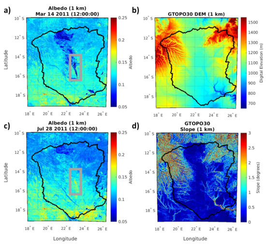
Figure 15.
Shortwave broadband albedo at noon local time for 2011 (a) after the peak of the rainy season and (c) during the dry season compared with the corresponding (b) elevations and (d) terrain slope analysis. The gray box outlines an area with higher than expected albedo values during the dry season.
3.4. Phase-Space Analysis
Phase-space maps of albedo, FVC, and SIF for miombo, grass savanna, and woody savanna across different years are shown in Figure 16 and Figure 17. Each point represents the mean value for all pixels of that land cover type, with colors representing the corresponding day of the year. The 95% confidence intervals were plotted as horizontal and vertical error bars, although many of the confidence interval values were so close to the mean that the short error bars were obscured by the markers. Dark blue shapes show the approximate form of each set of pixels, with arrows overlaid on the shapes to mark the direction of time. The offset between the two branches of the seasonal limit-cycle (“loop”) indicates the degree of hysteresis in the relationship between the two variables. The land cover classes used here incorporate dynamic wetland mapping since each point represents a 4-day (for graphs with LAI or FVC but without GOSIF) or 8-day (for graphs with GOSIF) time step, depending on which dataset has the coarser temporal resolution. This enables a more realistic comparison of the interactions between albedo, LAI, FVC, and SIF and rainfall variability for each land cover type as wetland areas become inundated.
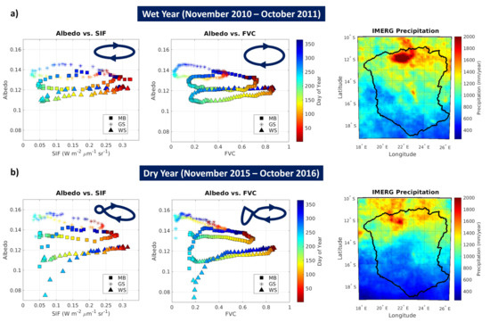
Figure 16.
Phase-space analysis of mean albedo, SIF, and FVC values for each land-cover class for (a) a wet year (2010–2011) and (b) a dry year (2015–2016) across miombo (MB), grass savanna (GS), and woody savanna (WS) land cover types. The accumulated annual precipitation for each year (consecutive rainy and dry seasons from November to October) is shown on the right-hand side for reference. Dark blue elliptical shapes represent the approximate shape of the limit-cycle and arrows indicate the direction of time. The 95% confidence interval values are plotted as horizontal and vertical error bars, with bar lengths representing the distance of the interval endpoints to the mean. Rainy season values in the phase-space diagrams are marked by the dark blue to dark red transition to the right of the graphs and dry season values are marked by the light blue to light green transition to the left of the graphs.
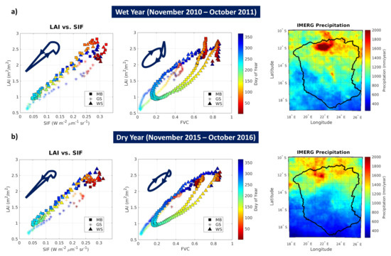
Figure 17.
Phase-space analysis of mean LAI, SIF, and FVC values for each land-cover class for (a) a wet year (2010–2011) and (b) a dry year (2015–2016) across miombo (MB), grass savanna (GS), and woody savanna (WS) land cover types. The accumulated annual precipitation for each year (consecutive rainy and dry seasons from November to October) is shown on the right-hand side for reference. Dark blue elliptical shapes represent the approximate shape of the limit-cycle and arrows indicate the direction of time. The 95% confidence interval values were plotted as horizontal and vertical error bars, with bar lengths representing the distance of the interval endpoints to the mean. Rainy season values in the phase-space diagrams are marked by the dark blue to dark red transition to the right of the graphs and dry season values are marked by the light blue to light green transition to the left of the graphs.
3.5. Seasonal Variability of Albedo
Across all land cover types, inspection of the smooth limit-cycles in Figure 16a indicates large hysteresis (offset of the trajectory in phase-space) consistent with strong seasonal patterns in the wet year and decreasing albedo in the rainy season (tied to increasing FVC and increased LAI and SIF in Figure 17a) with increasing albedo ranges from woody to grass savanna and miombo in-between. In the dry year, however, the limit-cycles collapse (Figure 16b) with flipped behavior for grass and woody savanna land cover types. For grass savanna, albedo decreases more dramatically in the wet season when the precipitation deficit is at a maximum during the dry year (see Table S2 in the Supplementary Materials) and darker, greener grass flushes the landscape. For woody savanna, the limit-cycles exhibit smaller hysteresis in dry conditions (Figure 16b). Thus, drought depresses the seasonality of albedo. Nevertheless, note that, while the albedo offset is reduced, the miombo limit-cycles are stable and exhibit seasonal hysteresis.
The collapse of the radiative hysteresis (albedo offset) under dry conditions during 2015–2016, particularly for grass savanna pixels, is indicative of the high vulnerability of this ecosystem to water stress. Indeed, Figure 18 compares the mean limit-cycle for grassland under wet and dry conditions with the limit-cycles for grassland in the areas that receive daily mid-day rainfall as per Lowman et al. (2018) [52]. Under dry conditions, the local afternoon rainfall is critical for grass sustainability. The decreased hysteresis offsets during 2015–2016 for woody savanna and miombo reflects the prominent decrease in precipitation in the northeastern portion of the UZRB during 2015–2016, where miombo and woody savanna dominate. As a result, reduced rainfall and soil moisture differences between seasons decrease the difference in albedo during transitional periods.
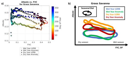
Figure 18.
(a) Phase-space analysis of mean albedo and FVC values for grass savanna pixels for a wet year (2010–2011) and a dry year (2015–2016) across the entire UZRB, as well as for the midland wetland area that receives localized precipitation (Anomaly) [52]. The 95% confidence interval values were plotted as horizontal and vertical error bars, with bar lengths representing the distance of the interval endpoints to the mean. (b) On the right is a conceptual diagram that synthesizes the impact of afternoon convection (Anomaly) produced by local circulations organized by land–atmosphere interactions and groundwater convergence [52] on the seasonal cycle of albedo. This shows the importance of landscape organization of water fluxes in producing hot-spots of enhanced ecosystem resilience.
The drop in albedo values for grass savanna in the southern portion of the basin could be due to the relative increase in the contribution of flooded dambos to the landscape-scale albedo when grass savanna is stressed under dry conditions in the rainy season of 2015–2016. These results suggest that these data capture both seasonal and interannual variability in response to the amount of precipitation in a given year.
3.6. Seasonal Variability of Vegetation
LAI, SIF, and FVC values were highest during the peak of the rainy season and lowest towards the end of the dry season. Both FVC and SIF values dropped close to 0 for grass savanna during the dry season, which can be explained by seasonal senescence characteristic of herbaceous vegetation in semi-arid regions [88]. Based on comparisons of the vegetation data depicted in Figure 17, the degree of hysteresis for each graph varied depending on the time of year and the land cover type. In general, LAI and SIF comparisons display a positive linear dependence without hysteresis for both miombo and woody savanna in the wet year. This behavior highlights increases in LAI due to increases in soil moisture that result in increased photosynthesis and SIF activity. Note however that, due to cloud cover in the rainy season, hysteresis emerges for grass savanna with the lower branch (lower LAI, lower SIF) in the wet season, highlighting seasonal increases in soil moisture in response to precipitation.
FVC saturates in the peak of the rainy season (cross-over loop). LAI and FVC comparisons indicate strong hysteresis for most of the year. The phase-space trajectories of (LAI, FVC) and (LAI, SIF) do not change significantly between the wet and dry year suggesting that they capture functional behavior of the three vegetation types, which could be used to parameterize regional phenology in models.
Woody savanna and miombo land cover exhibit similar LAI and SIF values, which can be explained by their similar root system structures. Notably, miombo pixels display enhanced hysteresis offsets compared to woody savanna pixels, emphasizing its more extensive lateral and deep root system [17]. Lateral roots near the surface effectively function as shallow grass roots because water does not have to infiltrate as deep into the soil to reach tap roots. Grass savanna has the strongest hysteresis during the rainy season, which is expected because the shallow root systems are more sensitive to changes in soil moisture. Near the surface, soil moisture is governed by rainfall variability because the topsoil is more susceptible to water loss through evaporation compared to deeper soils. In addition, the development of tap roots in woody savanna and miombo vegetation allow for root uptake of deep-water storage, resulting in a decreased sensitivity to changes in precipitation. Overall, hysteresis decreases between the wet and dry year, with greater impacts on grass savanna because of the higher soil moisture sensitivity due to the shallow root system characteristic of herbaceous vegetation [88].
3.7. Sources of Uncertainty
Although all data were interpolated or aggregated to 1 km spatial resolution for data analysis, Figure 19 illustrates how comparisons between coarser resolution (i.e., SIF in Figure 19a) and finer resolution (i.e., land cover in Figure 19b) data may decrease the accuracy of remotely-sensed land surface properties. Detailed, dynamic physical features such as wetland areal extent are lost as spatial resolution decreases, and smaller features such as dambos can be obscured even at 1 km resolution.
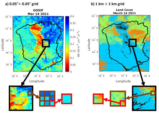
Figure 19.
Spatial resolution comparisons between (a) a 0.05° × 0.05° grid and (b) a 1 km × 1 km grid.
In addition, the shapes in Figure 17 resemble a cone and an ellipse for LAI vs. SIF and LAI vs. FVC, respectively, which appear as though they are folded over. The sharp drops in LAI during the peak of the rainy season indicate that the interpolation of widely variable LAI values in the TIMESAT cloud correction algorithm for each year could be skewed by outliers at the transition between calendar years (see the first data points of Figure 2b for woody savanna), resulting in LAI that is not representative of the landscape during the rainy season when cloud contamination issues are most severe. Figure 2a shows a decrease in LAI values to the east of the wetlands which may be a result of TIMESAT filtering at short time scales and cloud contamination. Increased values to the west of and within the wetlands after TIMESAT correction are a product of averaging in TIMESAT, suggesting a loss of information. Of the re-classified miombo pixels, mixed forest pixels (based on the original IGBP classification) are more influenced by averaging issues, while evergreen broadleaf pixel values (based on the original IGBP classification) are preserved (see Figure 3a of the stationary land cover for the original IGBP land cover classes).
3.8. Future Work
Future studies could further examine the changes in surface energy fluxes discussed in this paper by, for example, analyzing in situ data from flux-towers co-located with the three main ecosystems across the UZRB to examine the phase-space of radiative properties and vegetation phenology. Lowman et al. (2018) [52] used satellite data to specify vegetation parameters including radiative properties and compared their simulations using a hydrologic model with dynamic vegetation [90] against flux-tower data from Mongu, Zambia with good results (see their Figure 7). Lowman and Barros (2019) [91] added a predictive phenology module to the same model to simulate the feedbacks among vegetation dynamics, climate variability (temperature, humidity, and rainfall), and the surface energy budget to be compared against satellite and flux-tower observations. Furthermore, it would be interesting to examine the strength of local land–atmosphere coupling and to characterize the impact of changes in the spatial organization of albedo on the spatial organization of clouds and rainfall. Because of the large areal extent of savanna ecosystems and because seasonal changes in albedo imply seasonal changes in Bowen ratio, and therefore in low-level relative humidity and moist instability, there is also potential for regional impacts on convective activity tied to vegetation condition (e.g., [92,93]). Whereas previous studies have generally focused on humid climatic regions, the UZRB is located in a region of transition between the Congo River Basin and the Kalahari Desert.
Future work could also involve analyzing finer resolution (i.e., 30 m) Landsat imagery in addition to the land surface data examined in this manuscript to develop more dynamic land cover maps and improve comparisons across different land cover types. Agricultural areas are of great interest since local populations in the UZRB rely on subsistence agriculture. The land use and land cover changes associated with small-scale agriculture can have profound impacts on the water and surface energy balance in the region as population increases and climate change add additional stressors to food security [10,11,17,94,95]. A better understanding of the land–atmosphere feedbacks and natural system resiliency could inform climate-smart agricultural practices aligned with the United Nations Sustainable Development Goals to address climate mitigation, adaptation, and poverty reduction.
4. Conclusions
A joint, multi-sensor analysis of albedo, leaf area index, fractional vegetation cover, solar-induced chlorophyll fluorescence, and precipitation was conducted to understand how land surface properties are interrelated in maintaining the surface energy balance and water budget. The estimated albedo exhibit realistic diurnal cycles, and the results from the analysis indicate that strong seasonality and inter-annual variability in albedo are directly tied to landscape greening, and in particular soil moisture availability in the root zone and root water uptake following precipitation events. This study establishes regional-scale relationships that illustrate the functional behaviors of miombo, grass savanna, and woody savanna land cover types. Deep-rooted vegetation is less vulnerable to drought. Miombo exhibits optimal adaptive characteristics with robust seasonality for both dry and wet conditions in the region of study (see Figure 6). Operational phase-space analysis of albedo-FVC and albedo-SIF limit cycles can be used to monitor ecosystem stability and to detect changes. For example, grass savanna’s high vulnerability to water stress is indicative of potential run-away feedbacks of miombo deforestation.
Dambos (seasonal headwater wetlands) provide localized surface storage for runoff in this region. The hydrologic functionality of dambos is similar to flood irrigation with distributed runoff control, that is the natural system counterpart to micro-dams in small-holder agriculture [96]. Infiltration of ponded water recharges the water table and soil moisture in the rainy season; in the dry season, miombo’s deep roots physiologically pump water from deep soil layers upward that is then laterally redistributed at shallow soil depths. During the rainy season, miombo root systems anchor the soil catenas reducing erosion, and thus preserve the topsoil and landform. Dambos and miombo trees play therefore complementary roles in regional hydrology that increase the overall landscape resilience to water stress throughout the year.
The importance of dambos in food production in Southern Africa, and in particular Zambia, Zimbabwe, and Malawi, has long been studied (e.g., [22,97,98,99,100,101,102]). The synergy between miombo and dambos provides a framework for sustainable agriculture to emulate the resiliency of natural systems in this region. Indeed, recent data show significant increases in crop yield (30–60%) from cultivated dambos when miombo trees are preserved in the landscape as opposed to those that have been cleared [103].
In addition to increasing surface water storage through cultivated dambos, accessing blue water resources, or water withdrawn from surface water and aquifers without depleting environmental flows or groundwater, in a sustainable fashion is crucial for long-term agriculture. Economic water scarcity corresponds to conditions in which blue water resources are physically available, but society’s use of that water is hindered by the lack of institutional and economic capacity required to access such water resources [9,104,105,106]. Agricultural economically water scarce croplands are rainfed agricultural areas where sustainable irrigation expansion is suitable [9]. In Zimbabwe, irrigation by recharge from thousands of human-made earth micro-dams has long been recognized as key to high agricultural productivity [107,108,109]. Dambos play in natural systems an irrigation role not unlike the small earth dams in Zimbabwe farms. Abandonment and inadequate maintenance of these micro-dams in the last twenty years has been in large part associated with the severe decline in agricultural productivity (e.g., [107,108]). Therefore, prospects for long-term subsistence agriculture in the region encompass the preservation of dambos’ ecohydrological functionality.
As shown by Rosa et al. (2020) [9], croplands in the savannah ecosystems to the north and northeast of the Upper Zambezi River Basin experience agricultural economic water scarcity, particularly in the dry season. Irrigation expansion for Sub-Saharan croplands facing economically water scarce conditions along with sustainable deficit irrigation practices (i.e., irrigation that reduces blue water supply to below maximum levels and enables the growth of mildly water-stressed crops with minimized impact on crop yield) from areas not currently facing water scarcity such as the UZRB can generate enough food for 189–235 million more people with a roughly 24–96% increase in irrigation water consumption [9]. Adopting sustainable deficit irrigation practices in conjunction with cultivated shallow dambos and miombo trees can enhance the resilience of the ecosystem and surrounding communities, improving food and water security as climate hazards intensify in the coming years [1,9,103,110].
Supplementary Materials
The following are available online at https://www.mdpi.com/article/10.3390/rs13152954/s1, Table S1: Mean seasonal and annual accumulated precipitation for each land cover type, Table S2: Mean albedo values and accumulated precipitation (JFMA, MJJAS, and OND) for each land cover type.
Author Contributions
Conceptualization, A.P.B.; methodology, A.P.B. and T.M.W.; formal analysis and interpretation, T.M.W. and A.P.B.; resources, A.P.B.; data curation, T.M.W.; writing—original draft preparation, T.M.W.; writing—review and editing, A.P.B. and T.M.W.; visualization, T.M.W.; supervision and guidance, A.P.B.; project administration, A.P.B.; funding acquisition, A.P.B. and T.M.W. Both authors have read and agreed to the published version of the manuscript.
Funding
This research was funded in part by the National Aeronautics and Space Administration, under grant numbers 80NSSC19K0685 and NNX17AL44G, and the Duke Pratt Research Fellows Program.
Institutional Review Board Statement
Not applicable.
Informed Consent Statement
Not applicable.
Data Availability Statement
MODIS data and FLDAS Noah data are available from the NASA Earthdata (https://earthdata.nasa.gov/, accessed on 9 July 2019–8 May 2020). GTOPO30 DEM data are available from USGS EarthExplorer (https://earthexplorer.usgs.gov/, accessed on 2 January 2020). GOSIF data are available from the Global Ecology Group Data Repository https://globalecology.unh.edu/data/GOSIF.html, accessed on 3 April 2020). OCO-2 SIF data are available from GESDISC (https://disc.gsfc.nasa.gov/datasets/OCO2_L2_Lite_SIF_10r/summary?keywords=OCO-2%20v10r, accessed on 15 May 2020). IMERG precipitation data are available from NASA’s PPS STORM data access interface (https://storm.pps.eosdis.nasa.gov/storm/, accessed on 24 February 2020).
Acknowledgments
The authors would like to thank the reviewers for their helpful comments and constructive criticisms of this manuscript. Lauren E.L. Lowman, as well as other past and present members of the Barros Research Group (Malarvizhi Arulraj, Masih Eghdami, Steven Chavez, Yueqian Cao, Mochi Liao, and others), provided invaluable guidance to T.M.W. in the early stages of this work.
Conflicts of Interest
The authors declare no conflict of interest. The funders had no role in the design of the study; in the collection, analyses, or interpretation of data; in the writing of the manuscript, or in the decision to publish the results.
Abbreviations
The following abbreviations are used in this manuscript:
| AOD | aerosol optical depth |
| BRDF | bi-directional reflectance distribution function |
| BRF | bi-directional reflectance factor |
| BSA | black-sky albedo |
| CNES | Centre National D’Etudes Spatiales (National Centre for Space Studies) |
| DEM | Digital Elevation Model |
| FEWS NET | Famine Early Warning Systems Network |
| FLDAS | FEWS NET Land Data Assimilation System |
| FVC | fractional vegetation cover |
| GEBCO | General Bathymetric Chart of the Oceans |
| GES DISC | Goddard Earth Sciences (GES) Data and Information Services Center (DISC) |
| GIS | Geographic Information System |
| GOSIF | Global ’OCO-2’ Solar-Induced chlorophyll Fluorescence |
| GPP | gross primary productivity |
| GTOPO30 | Global 30 Arc-Second Elevation |
| HEG | HDF-EOS to GeoTIFF |
| HEG-C | HDF-EOS to GeoTIFF Converter |
| HDF-EOS | Hierarchical Data Format - Earth Observing System |
| IBCAO | International Bathymetric Chart of the Arctic Ocean |
| IGBP | International Geosphere-Biosphere Programme |
| IMERG | Integrated Multi-satellitE Retrievals for Global Precipitation Measurement |
| ITCZ | Inter-Tropical Convergence Zone |
| JFMA | January, February, March, and April |
| LAI | Leaf Area Index |
| MAIAC | Multi-Angle Implementation of Atmospheric Correction |
| MERRA-2 | Modern-Era Retrospective Analysis for Research and Applications, Version 2 |
| MIR | Mid-Infrared Reflectance |
| MJJAS | May, June, July, August, and September |
| MODIS | Moderate Resolution Imaging Spectroradiometer |
| MRT | MODIS Reprojection Tool |
| MSL | Mean Sea Level |
| NASA | National Aeronautics and Space Administration |
| NDVI | Normalized Difference Vegetation Index |
| NDWI | Normalized Difference Water Index |
| NGA | National Geospatial-Intelligence Agency |
| NIR | Near-Infrared Reflectance |
| NOAA | National Oceanic and Atmospheric Administration |
| NREL SPA | National Renewable Energy Laboratory’s Solar Position Algorithm |
| OCO-2 | Orbiting Carbon Observatory-2 |
| OND | October, November, and December |
| PBL | Planetary Boundary Layer |
| PPS | Precipitation Processing System |
| QA | Quality Assurance |
| QC | Quality Control |
| QGIS | Quantum Geographic Information System |
| RTLS | Ross-Thick Li-Sparse Reciprocal |
| SIF | Solar-Induced Chlorophyll Fluorescence |
| SIN | MODIS SINusoidal Projection |
| SKYL | fraction of diffuse SKYLight |
| STORM | Science Team On-Line Request Module |
| SZA | Solar Zenith Angle |
| TC | Tasseled Cap |
| USGS | United States Geological Survey |
| UTM | Universal Transverse Mercator |
| UZRB | Upper Zambezi River Basin |
| WSA | White-Sky Albedo |
Appendix A. Wetland Probability Mapping Algorithm
Using seven bands of TIMESAT-corrected MODIS MCD43A4 Version 6 Nadir BRDF-adjusted reflectance data (Table A1), several indices sensitive to the greenness and water content of the surface were tested to determine how well they predicted the dynamic wetland areal extent using a similar methodology as Lowman et al. (2018) [52]. Stationary MODIS MCD12Q1 Version 6 land cover data from consecutive years with the largest permanent wetland area (2010–2012) were used to create training data of each index, and, based on how well the peaks of wetland and non-wetland pixels were separated in the histograms in Figure 3, five wetland predictor variables were selected: Near-Infrared Reflectance (NIR, or MODIS Band 2), the Normalized Difference Water Index (NDWI), Tasseled Cap (TC) Brightness, TC Greenness, and TC Wetness. These indices, described in Equations (A1) and (A2), were incorporated into a logistic regression model (Equations (A3) and (A4)) to produce seasonally-varying wetland maps.
where is the normalized difference water index, is MODIS reflectance Band 4 representing green light, and is MODIS reflectance Band 6 representing mid-infrared light [111].
where is the tasseled cap index value for index x () and is the tasseled cap coefficient for MODIS band i. MODIS instrument specifications and TC index coefficients are presented in Table A1.
where is the probability that wetland area is present within a given pixel based on predictor variables X and is the regression coefficient for predictor variable x representing the variable’s weight toward the resulting wetland presence probability [52]. Based on the intersection of the stationary wetland area line with the threshold-area curves for the three wet years (2010–2012) in Figure 3b, a 99% probability threshold was selected to determine where wetland areas were located.
Table A1.
MODIS instrument specifications and tasseled cap coefficients from [112].
Table A1.
MODIS instrument specifications and tasseled cap coefficients from [112].
| MODIS Band | Wavelength (nm) | Light | Brightness () | Greenness () | Wetness () |
|---|---|---|---|---|---|
| 1 | 620–670 | Red | 0.4395 | −0.4064 | 0.1147 |
| 2 | 841–876 | Near-infrared (NIR) | 0.5945 | 0.5129 | 0.2489 |
| 3 | 459–479 | Blue | 0.2460 | −0.2744 | 0.2408 |
| 4 | 545–565 | Green | 0.3918 | −0.2893 | 0.3132 |
| 5 | 1230–1250 | Near-infrared (NIR) | 0.3506 | 0.4882 | −0.3122 |
| 6 | 1628–1652 | Mid-infrared (MIR) | 0.2136 | −0.0036 | −0.6416 |
| 7 | 2105–2155 | Mid-infrared (MIR) | 0.2678 | −0.4169 | −0.5087 |
References
- Mora, C.; Spirandelli, D.; Franklin, E.C.; Lynham, J.; Kantar, M.B.; Miles, W.; Smith, C.Z.; Freel, K.; Moy, J.; Louis, L.V.; et al. Broad threat to humanity from cumulative climate hazards intensified by greenhouse gas emissions. Nat. Clim. Chang. 2018, 8, 1062–1071. [Google Scholar] [CrossRef]
- Van Loon, A.F.; Stahl, K.; Di Baldassarre, G.; Clark, J.; Rangecroft, S.; Wanders, N.; Gleeson, T.; Van Dijk, A.I.J.M.; Tallaksen, L.M.; Hannaford, J.; et al. Drought in a human-modified world: Reframing drought definitions, understanding, and analysis approaches. Hydrol. Earth Syst. Sci. 2016, 20, 3631–3650. [Google Scholar] [CrossRef] [Green Version]
- Foley, J.A.; DeFries, R.; Asner, G.P.; Barford, C.; Bonan, G.; Carpenter, S.R.; Chapin, F.S.; Coe, M.T.; Daily, G.C.; Gibbs, H.K.; et al. Global consequences of land use. J. Sci. 2005, 309, 570–574. [Google Scholar] [CrossRef] [PubMed] [Green Version]
- Gordon, L.J.; Peterson, G.D.; Bennett, E.M. Agricultural modifications of hydrological flows create ecological surprises. Trends Ecol. Evol. 2008, 23, 211–219. [Google Scholar] [CrossRef] [PubMed]
- Sheffield, J.; Wood, E.F.; Chaney, N.; Guan, K.; Sadri, S.; Yuan, X.; Olang, L.; Amani, A.; Ali, A.; Demuth, S.; et al. A Drought Monitoring and Forecasting System for Sub-Sahara African Water Resources and Food Security. Bull. Am. Meteorol. Soc. 2014, 95, 861–882. [Google Scholar] [CrossRef]
- UN/ISDR. Drought Risk Reduction Framework and Practices: Contributing to the Implementation of the Hyogo Framework for Action; United Nations Secretariat of the International Strategy for Disaster Reduction: Geneva, Switzerland, 2009; p. 197. [Google Scholar]
- Hanasaki, N.; Fujimori, S.; Yamamoto, T.; Yoshikawa, S.; Masaki, Y.; Hijioka, Y.; Kainuma, M.; Kanamori, Y.; Masui, T.; Takahashi, K.; et al. A global water scarcity assessment under Shared Socio-economic Pathways—Part 2: Water availability and scarcity. Hydrol. Earth Syst. Sci. 2013, 17, 2393–2413. [Google Scholar] [CrossRef] [Green Version]
- Calow, R.C.; MacDonald, A.M.; Nicol, A.L.; Robins, N.S. Ground water security and drought in Africa: Linking availability, access, and demand. Ground Water 2010, 48, 246–256. [Google Scholar] [CrossRef]
- Rosa, L.; Chiarelli, D.D.; Rulli, M.C.; Dell’Angelo, J.; D’Odorico, P. Global agricultural economic water scarcity. Sci. Adv. 2020, 6, eaaz6031. [Google Scholar] [CrossRef]
- Nhemachena, C.; Nhamo, L.; Matchaya, G.; Nhemachena, C.R.; Muchara, B.; Karuaihe, S.T.; Mpandeli, S. Climate Change Impacts on Water and Agriculture Sectors in Southern Africa: Threats and Opportunities for Sustainable Development. Water 2020, 12, 2673. [Google Scholar] [CrossRef]
- Nhamo, L.; Mabhaudhi, T.; Modi, A. Preparedness or repeated short-term relief aid? Building drought resilience through early warning in southern Africa. Water SA 2019, 45, 75–85. [Google Scholar] [CrossRef] [Green Version]
- Nhamo, L.; Matchaya, G.; Mabhaudhi, T.; Nhlengethwa, S.; Nhemachena, C.; Mpandeli, S. Cereal production trends under climate change: Impacts and adaptation strategies in southern Africa. Agriculture 2019, 9, 30. [Google Scholar] [CrossRef] [Green Version]
- Rockstrom, J. Water resources management in smallholder farms in Eastern and Southern Africa: An overview. Phys. Chem. Earth Part B Hydrol. Ocean. Atmos. 2000, 25, 275–283. [Google Scholar] [CrossRef]
- Bagley, J.E.; Desai, A.R.; Dirmeyer, P.A.; Foley, J.A. Effects of land cover change on moisture availability and potential crop yield in the world’s breadbaskets. Environ. Res. Lett. 2012, 7, 014009. [Google Scholar] [CrossRef]
- Dwivedi, S. Sahrawat, K.; Upadhyaya, H.; Ortiz, R. Food, nutrition and agrobiodiversity under global climate change. Adv. Agron. 2013, 120. [Google Scholar] [CrossRef] [Green Version]
- Marvin, H.J.P.; Kleter, G.A.; Van der Fels-Klerx, H.J.; Noordam, M.Y.; Franz, E.; Willems, D.J.M.; Boxall, A. Proactive systems for early warning potential impacts of natural disasters on food safety: Climate-change-induced extreme events as case in point. Food Control 2013, 34, 444–456. [Google Scholar] [CrossRef]
- Desanker, P.V.; Frost, P.G.H.; Frost, C.O.; Justice, C.O.; Scholes, R.J. The Miombo Network: Framework for a Terrestrial Transect Study of Land-Use and Land-Cover Change in the Miombo Ecosystems of Central Africa; IGBP Report 41; The International Geosphere-Biosphere Programme: Stockholm, Sweden, 1997; pp. 9–22. [Google Scholar]
- Frost, P. The ecology of miombo woodlands. In The Miombo in Transition: Woodlands and Welfare in Africa; Campbell, B., Ed.; Centre for International Forestry Research: Bogor, Indonesia, 1996. [Google Scholar]
- Scholes, R.J. Carbon storage in Southern African woodlands. In Indigenous Forests and Woodlands in South Africa; Lawes, M.J., Eeley, H.A.C., Shackleton, C.M., Geach, B.G.S., Eds.; University of Kwazulu-Natal Press: Pietermaritzburg, South Africa, 2004; Chapter 29. [Google Scholar]
- Syampungani, S. The miombo woodlands at the cross roads: Potential threats, sustainable livelihoods, policy gaps and challenges. Nat. Resour. Forum 2009, 33, 150–159. [Google Scholar] [CrossRef]
- Wilson, S.A.; Scholes, R.J. The climate impact of land use change in the miombo region of south central Africa. J. Integr. Environ. Sci. 2020, 17, 187–203. [Google Scholar] [CrossRef]
- Dewees, P.A.; Campbell, B.M.; Katerere, Y.; Sitoe, A.; Cunningham, A.B.; Angelsen, A.; Wunder, S. Managing the Miombo Woodlands of Southern Africa: Policies, Incentives, and Options for the Rural Poor. J. Nat. Resour. Pol’y Res. 2010, 2, 57–73. [Google Scholar] [CrossRef] [Green Version]
- Lupala, Z.J.; Lusambo, L.P.; Ngaga, Y.M.; Makatta, A.A. The Land Use and Cover Change in Miombo Woodlands under Community Based Forest Management and Its Implication to Climate Change Mitigation: A Case of Southern Highlands of Tanzania. Int. J. For. Res. 2015, 2015. [Google Scholar] [CrossRef] [Green Version]
- Wily, L.; Dewees, P.A. From Users to Custodians: Changing Relations Between People and the State in Forest Management in Tanzania; World Bank Publications: Washington, DC, USA, 2001; Volume 2569. [Google Scholar]
- Ellis, J.; Galvin, K.A. Climate patterns and land-use practices in the dry zones of Africa. Bioscience 1994, 44, 340–349. [Google Scholar] [CrossRef]
- Sedano, F.; Gong, P.; Ferrão, M. Land cover assessment with MODIS imagery in southern African Miombo ecosystems. Remote Sens. Environ. 2005, 98, 429–441. [Google Scholar] [CrossRef]
- Grace, J.; José, J.S.; Meir, P.; Miranda, H.S.; Montes, R.A. Productivity and carbon fluxes of tropical savannas. J. Biogeogr. 2006, 33, 387–400. [Google Scholar] [CrossRef]
- Williams, M.; Ryan, C.M.; Rees, R.M.; Sambane, E.; Fernando, J.; Grace, J. Carbon sequestration and biodiversity of re-growing miombo woodlands in Mozambique. For. Ecol. Manag. 2006, 254, 145–155. [Google Scholar] [CrossRef]
- Greig-Smith, P. Pattern in vegetation. J. Ecol. 1979, 67, 755–779. [Google Scholar] [CrossRef]
- Schlesinger, W.H.; Reynolds, J.F.; Cunningham, G.L.; Huenneke, L.F.; Jarrel, W.M.; Virginia, R.A.; Whitford, W.G. Biological feedbacks in global desertification. Science 1990, 147, 1043–1048. [Google Scholar] [CrossRef] [Green Version]
- Belsky, A.J. Influences of trees on savanna productivity: Tests of shade, nutrients, and tree-grass competition. Ecology 1994, 75, 922–932. [Google Scholar] [CrossRef]
- Greene, R.S.B.; Valentin, C.; Esteves, M. Runoff and erosion processes. In Banded Vegetation Patterning in Arid and Semiarid Environment; Tongway, D.J., Valentin, C., Seghieri, J., Eds.; Springer: New York, NY, USA, 2001; pp. 52–77. [Google Scholar] [CrossRef]
- D’Odorico, P.; Caylor, K.; Okin, G.S.; Scanlon, T.M. On soil moisture-vegetation feedbacks and their possible effects on the dynamics of dryland ecosystems. J. Geophys. Res. 2007, 112, G04010. [Google Scholar] [CrossRef]
- Walker, B.H.; Ludwig, D.; Holling, C.S.; Peterman, R.M. Stability of semiarid savanna grazing systems. J. Ecol. 1981, 69, 473–498. [Google Scholar] [CrossRef]
- Greene, R.S.B. Soil physical properties of three geomorphic zones in a semiarid mulga woodland. Aust. J. Soil. Res. 1992, 30, 55–69. [Google Scholar] [CrossRef]
- Greene, R.S.B.; Kinnell, P.I.A.; Wood, J.T. Role of plant cover and stock trampling on runoff and soil erosion from semiarid wooded rangelands. Aust. J. Soil. Res. 1994, 32, 953–973. [Google Scholar] [CrossRef]
- Breman, H.; Kessler, J.J. Woody Plants in Agro-Ecosystems of Semi-Arid Regions; Springer: New York, NY, USA, 1995; p. 340. [Google Scholar]
- Scholes, R.J.; Archer, S.R. Tree-grass interactions in savannas. Annu. Rev. Ecol. Syst. 1997, 28, 517–544. [Google Scholar] [CrossRef]
- Bhark, E.W.; Small, E.E. Association between plant canopies and the spatial patterns of infiltration in shrubland and grassland of the Chihuahuan desert, New Mexico. Ecosystems 2003, 6, 185–196. [Google Scholar] [CrossRef]
- Zeng, Q.-C.; Zeng, X.D. An analytical dynamic model of grass field ecosystem with two variables. Ecol. Model. 1996, 85, 187–196. [Google Scholar] [CrossRef]
- Zeng, X.; Shen, S.S.P.; Zeng, X.; Dickinson, R.E. Multiple equilibrium states and the abrupt transitions in a dynamical system of soil water interacting with vegetation. Geophys. Res. Lett. 2004, 31, L05501. [Google Scholar] [CrossRef] [Green Version]
- Govaerts, Y.; Lattanzio, A. Estimation of surface albedo increase during the eighties Sahel drought from Meteosat observations. Glob. Planet. Chang. 2008, 64, 139–145. [Google Scholar] [CrossRef]
- Pinty, B.; Verstraete, M.; Gobron, N.; Govaerts, Y.; Roveda, F. Do man-made fires affect Earth’s surface reflectance at continental scales? EOS Trans. AGU 2011, 81, 381–389. [Google Scholar] [CrossRef]
- Segal, M.; Avissar, R.; McCumber, M.C.; Pielke, R.A. Evaluation of Vegetation Effects on the Generation and Modification of Mesoscale Circulations. J. Atmos. Sci. 1988, 45, 2268–2293. [Google Scholar] [CrossRef] [Green Version]
- Santanello, J.A., Jr.; Dirmeyer, P.A.; Ferguson, C.R.; Findell, K.L.; Tawfik, A.B.; Berg, A.; Ek, M.; Gentine, P.; Guillod, B.P.; van Heerwaarden, C.; et al. Land-Atmosphere Interactions: The LoCo Perspective. Bull. Am. Meteorol. Soc. 2018, 99, 1253–1272. [Google Scholar] [CrossRef]
- Eghdami, M.; Barros, A.P. Deforestation Impacts on Orographic Precipitation in the Tropical Andes. Front. Environ. Sci. 2020, 8, 580159. [Google Scholar] [CrossRef]
- Tao, J.; Barros, A.P. Multi-year surface radiative properties and vegetation parameters for hydrologic modeling on regions of complex terrain methodology and evaluation over the Integrated Precipitation and Hydrology Experiment 2014 domain. J. Hydrol. 2019, 22, 100596. [Google Scholar] [CrossRef]
- Liang, S. Narrowband to broadband conversions of land surface albedo I: Algorithms. Remote Sens. Environ. 2001, 70, 29–51. [Google Scholar] [CrossRef]
- Lyapustin, A.; Wang, Y. MAIAC: Multi-Angle Implementation of Atmospheric Correction for MODIS; Algorithm Theoretical Basis Document Version 1.0; Goddard Earth Science and Technology Center UMBC and NASA GSFC: Greenbelt, MD, USA, 1992; pp. 1–77. Available online: https://modis-land.gsfc.nasa.gov/pdf/MAIAC_ATBD_v1.pdf (accessed on 19 July 2019).
- Gitelson, A.A.; Kaufman, Y.J.; Stark, R.; Rundquist, D. Novel algorithms for remote estimation of vegetation fraction. Remote Sens. Environ. 2002, 80, 76–87. [Google Scholar] [CrossRef] [Green Version]
- Meroni, M.; Rossini, M.; Guanter, L.; Alonso, L.; Rascher, U.; Colombo, R.; Moreno, J. Remote sensing of solar-induced chlorophyll fluorescence: Review of methods and applications. Remote Sens. Environ. 2009, 113, 2037–2051. [Google Scholar] [CrossRef]
- Lowman, L.E.L.; Wei, T.M.; Barros, A.P. Rainfall variability, wetland persistence, and water-carbon cycle coupling in the Upper Zambezi River Basin in Southern Africa. Remote Sens. 2018, 10, 692. [Google Scholar] [CrossRef] [Green Version]
- Madani, N.; Kimball, J.S.; Jones, L.A.; Parazoo, N.C.; Guan, K. Global Analysis of Bioclimatic Controls on Ecosystem Productivity Using Satellite Observations of Solar-Induced Chlorophyll Fluorescence. Remote Sens. 2017, 9, 530. [Google Scholar] [CrossRef] [Green Version]
- Waliser, D.E.; Gautier, C. A satellite-derived climatology of the ITCZ. J. Clim. 1993, 6, 2162–2174. [Google Scholar] [CrossRef]
- Winsemius, H.C.; Savenije, H.H.G.; Gerrits, A.M.J.; Zapreeva, E.A.; Klees, R. Comparison of two model approaches in the Zambezi river basin with regard to model reliability and identifiability. Hydrol. Earth Syst. Sci. 2005, 2, 2625–2661. [Google Scholar] [CrossRef] [Green Version]
- HDF-EOS to GeoTIFF Converter (HEG-C), v2.14. Distributed by Earth Science Data and Information System (ESDIS) Project, Earth Science Projects Division (ESPD), Flight Projects Directorate, Goddard Space Flight Center (GFSC) National Aeronautics and Space Administration (NASA). 2017. Available online: https://wiki.earthdata.nasa.gov/display/DAS/HEG%3A++HDF-EOS+to+GeoTIFF+Conversion+Tool (accessed on 4 June 2019).
- Jönsson, P.; Eklundh, L. TIMESAT—A program for analyzing time series of satellite sensor data. Comput. Geosci. 2005, 30, 833–845. [Google Scholar] [CrossRef] [Green Version]
- Friedl, M.; Sulla-Menashe, D. MCD12Q1 MODIS/Terra + Aqua Land Cover Type Yearly L3 Global 500 m SIN grid V006. 2019; Distributed by NASA EOSDIS Land Processes DAAC. Available online: https://lpdaac.usgs.gov/products/mcd12q1v006/ (accessed on 8 May 2020).
- Schaaf, C.; Wang, Z. MCD43A4 MODIS/Terra+Aqua BRDF/Albedo Nadir BRDF Adjusted Ref Daily L3 Global—500 m V006. 2015; Distributed by NASA EOSDIS Land Processes DAAC. Available online: https://lpdaac.usgs.gov/products/mcd43a4v006/ (accessed on 22 February 2020).
- Schaaf, C.; Wang, Z. MCD43A2 MODIS/Terra+Aqua BRDF/Albedo Quality Daily L3 Global—500 m V006. 2015; Distributed by NASA EOSDIS Land Processes DAAC. Available online: https://lpdaac.usgs.gov/products/mcd43a2v006/ (accessed on 22 February 2020).
- Lyapustin, A.; Wang, Y. MCD19A2 MODIS/Terra+Aqua Land Aerosol Optical Depth Daily L2G Global 1 km SIN Grid V006. 2018; Distributed by NASA EOSDIS Land Processes DAAC. Available online: https://lpdaac.usgs.gov/products/mcd19a2v006/ (accessed on 9 July 2019).
- Lyapustin, A.; Wang, Y. MCD19A3 MODIS/Terra+Aqua BRDF Model Parameters 8-Day L3 Global 1 km SIN Grid V006. 2018; Distributed by NASA EOSDIS Land Processes DAAC. Available online: https://lpdaac.usgs.gov/products/mcd19a3v006/ (accessed on 27 April 2020).
- Wan, Z.; Hook, S.; Hully, G. MOD11A1 MODIS/Terra Land Surface Temperature/Emissivity Daily L3 Global 1 km SIN Grid V006. 2015; Distributed by NASA EOSDIS Land Processes DAAC. Available online: https://lpdaac.usgs.gov/products/mod11a1v006/ (accessed on 16 December 2019).
- Wan, Z.; Hook, S.; Hully, G. MYD11A1 MODIS/Aqua Land Surface Temperature/Emissivity Daily L3 Global 1 km SIN Grid V006. 2015; Distributed by NASA EOSDIS Land Processes DAAC. Available online: https://lpdaac.usgs.gov/products/myd11a1v006/ (accessed on 16 December 2019).
- Myneni, R.; Knyazikhin, Y.; Park, T. MCD15A3H MODIS/Terra+Aqua Leaf Area Index/FPAR 4-day L4 Global 500 m SIN Grid V006. 2015; Distributed by NASA EOSDIS Land Processes DAAC. Available online: https://lpdaac.usgs.gov/products/mcd15a3hv006/ (accessed on 18 December 2019).
- McNally, A. FLDAS Noah Land Surface Model L4 Global Monthly 0.1 × 0.1 degree (MERRA-2 and CHIRPS). 2018; Distributed by Goddard Earth Sciences Data and Information Services Center (GES DISC). Available online: https://cmr.earthdata.nasa.gov/search/concepts/C1563089663-GES_DISC.html (accessed on 8 May 2020).
- Earth Resources Observation and Science Center, U.S. Geological Survey, U.S. Department of the Interior. USGS 30 ARC-second Global Elevation Data, GTOPO30. 1997; Distributed by Research Data Archive at the National Center for Atmospheric Research, Computational and Information Systems Laboratory. Available online: https://www.usgs.gov/centers/eros/science/usgs-eros-archive-digital-elevation-global-30-arc-second-elevation-gtopo30?qt-science_center_objects=0#qt-science_center_objects (accessed on 2 January 2020).
- Li, X.; Xiao, J. A global, 0.05-degree product of solar-induced chlorophyll fluorescence derived from OCO-2, MODIS, and reanalysis data. Remote Sens. 2019, 11, 571. [Google Scholar] [CrossRef] [Green Version]
- OCO-2 Science Team; Gunson, M.; Eldering, A. OCO-2 Level 2 Bias-Corrected Solar-Induced Fluorescence and Other Select Fields from the IMAP-DOAS Algorithm Aggregated as Daily Files, Retrospective Processing V10r. 2020; Distributed by Goddard Earth Sciences Data and Information Services Center (GES DISC). Available online: https://disc.gsfc.nasa.gov/datasets/OCO2_L2_Lite_SIF_10r/summary (accessed on 15 May 2020).
- Huffman, G.J.; Stocker, E.F.; Bolvin, D.T.; Nelkin, E.J.; Tan, J. GPM_3IMERGM. Version 06. GPM IMERG Final Precipitation L3 1 Month 0.1 Degree × 0.1 Degree V06. 2019 Distributed by National Aeronautics and Space Administration, U.S. Government, Goddard Earth Sciences Data and Information Services Center (GES DISC). Available online: https://disc.gsfc.nasa.gov/datasets/GPM_3IMERGM_06/summary (accessed on 24 February 2020).
- About Terra. Available online: https://terra.nasa.gov/about (accessed on 25 July 2021).
- Aqua Earth-Observing Satellite Mission. Available online: https://aqua.nasa.gov/ (accessed on 25 July 2021).
- Bréda, N.J.J. Ground-based measurements of leaf area index: A review of methods, instruments and current controversies. J. Exp. Bot. 2003, 54, 2403–2417. [Google Scholar] [CrossRef]
- Gower, S.T.; Kucharik, C.J.; Norman, J. M Direct and indirect estimation of leaf area index, fAPAR, and net primary production of terrestrial ecosystems. Remote Sens. Environ. 1999, 70, 29–51. [Google Scholar] [CrossRef]
- Carlson, T.N.; Ripley, D.A. On the relation between NDVI, fractional vegetation cover, and leaf area index. Remote Sens. Environ. 1997, 62, 241–252. [Google Scholar] [CrossRef]
- Huete, A.; Didan, K.; van Leeuwen, W.; Miura, T.; Glenn, E. MODIS Vegetation Indices. In Land Remote Sensing and Global Environmental Change. Remote Sensing and Digital Image Processing; Ramachandran, B., Justice, C.O., Abrams, M.J., Eds.; Springer: New York, NY, USA, 2010; Volume 11, pp. 579–602. [Google Scholar] [CrossRef]
- Ribeiro, N.; Cumbana, M.; Mamugy, F.; Chaúque, A. Remote Sensing of Biomass in the Miombo Woodlands of Southern Africa: Opportunities and Limitations for Research. In Remote Sensing of Biomass, Principles and Applications; Fatoyinbo, T., Ed.; InTech: Rijeka, Croatia, 2012; Chapter 4; pp. 77–98. [Google Scholar]
- White, F. The Vegetation of Africa; United Nations Educational: Paris, France, 1983; Volume 20, p. 356. [Google Scholar]
- Chidumayo, E.N. Management implications of tree growth patterns in miombo woodlands of Zambia. For. Ecol. Manag. 2019, 436, 105–116. [Google Scholar] [CrossRef]
- O’Donnell, F.C.; Caylor, K.K.; Bhattachan, A.; Dintwe, K.; D’Odorico, P.; Okin, G.S. A quantitative description of the interspecies diversity of belowground structure in savanna woody plants. Ecosphere 2015, 6, 154. [Google Scholar] [CrossRef]
- Google Earth: Upper Zambezi River Basin. Available online: https://earth.google.com/web/@-14.89112745,21.94883161,1080.78154958a,1996566.68945879d,35y,0h,0t,0r (accessed on 23 April 2020).
- Tao, J.; Barros, A.P. The Integrated Precipitation and Hydrology Experiment, Part I: Quality High-Resolution Landscape Attributes Datasets; Report No. EPL-2013-IPHEx-H4SE-I; EPL/Duke University: Durham, NC, USA, 2013; p. 60. Available online: https://dukespace.lib.duke.edu/dspace/handle/10161/8289 (accessed on 3 August 2018).
- Schaaf, C.B.; Gao, F.; Strahler, A.H.; Lucht, W.; Li, X.; Tsang, T.; Strugnell, N.C.; Zhang, X.; Jin, Y.; Muller, J.-P.; et al. First operational BRDF, albedo nadir reflectance products from MODIS. Remote Sens. Environ. 2002, 83, 135–148. [Google Scholar] [CrossRef] [Green Version]
- Reda, I.; Andreas, A. Solar Position Algorithm for Solar Radiation Applications; Report No. TPL-560-34302; National Renewable Energy Laboratory: Golden, CO, USA, 2008; pp. 1–16. Available online: https://www.nrel.gov/docs/fy08osti/34302.pdf (accessed on 10 July 2019).
- Strahler, A.H.; Muller, J.-P. MODIS BRDF/Albedo Product; Algorithm Theoretical Basis Document Version 5.0; MODIS Science Team, MD, USA; 1999; pp. 1–53. Available online: https://modis.gsfc.nasa.gov/data/atbd/atbd_mod09.pdf (accessed on 19 July 2019).
- MODIS User Tools. Available online: https://www.umb.edu/spectralmass/terra_aqua_modis/modis_user_tools (accessed on 23 April 2020).
- Frankenberg, C. Solar Induced Chlorophyll Fluorescence OCO-2 Lite Files (B7000) User Guide; California Institute of Technology: Pasedena, CA, USA, 2015; pp. 1–9. Available online: https://docserver.gesdisc.eosdis.nasa.gov/public/project/OCO/OCO2_SIF_B7000_Product_Description_090215.pdf (accessed on 2 December 2019).
- Brandt, M.; Hiernaux, P.; Tagesson, T.; Verger, A.; Rasmussen, K.; Diouf, A.A.; Mbow, C.; Mougin, E.; Fensholt, R. Woody plant cover estimation in drylands from Earth Observation based seasonal metrics. Remote Sens. Environ. 2016, 172, 28–38. [Google Scholar] [CrossRef] [Green Version]
- McMahon, A.; Moore, R.D. Influence of turbidity and aeration on the albedo of mountain streams. Hydrol. Process. 2017, 31, 4477–4491. [Google Scholar] [CrossRef] [Green Version]
- Garcia-Quijano, J.F.; Barros, A.P. Incorporating canopy physiology into a hydrological model: Photosynthesis, dynamic respiration, and stomatal sensitivity. Ecol. Modell. 2005, 185, 29–49. [Google Scholar] [CrossRef]
- Lowman, L.E.L.; Barros, A.P. Fire-induced canopy changes alter plant water, energy and carbon relations for Coastal Plains Forests in the Southeast US. In Proceedings of the AGU Fall Meeting Abstracts, San Francisco, CA, USA, 9–13 December 2019; Volume 2019, p. B53H-2500. [Google Scholar]
- Barros, A.P.; Hwu, W. A study of land-atmosphere interactions during summertime rainfall using a mesoscale model. J. Geophys. Res. Atmos. 2002, 107. [Google Scholar] [CrossRef]
- Erlingis, J.M.; Barros, A.P. A study of the role of daytime land-atmosphere interactions on nocturnal convective activity in the southern Great Plains during CLASIC. J. Hydrometeorol. 2014, 15, 1932–1953. [Google Scholar] [CrossRef]
- Graham, C. Climate-induced population displacement in sub-Saharan Africa: A review of resilience-building strategies. Geoforum 2020, 117, 300–303. [Google Scholar] [CrossRef]
- Newell, P.; Taylor, O.; Naess, L.O.; Thompson, J.; Mahmoud, H.; Ndaki, P.; Rurangwa, R.; Teshome, A. Climate Smart Agriculture? Governing the Sustainable Development Goals in Sub-Saharan Africa. Front. Sustain. Food Syst. 2019, 3, 55. [Google Scholar] [CrossRef] [Green Version]
- Keshavarz, M.S.; Ebrahimian, H.; Abbasi, F.; Playán, E. Effect of micro-dams on water flow characteristics in furrow irrigation. Irrig. Sci. 2020, 38, 307–319. [Google Scholar] [CrossRef]
- Turner, B. The importance of dambos in African agriculture. Land Use Policy 1986, 3, 343–347. [Google Scholar] [CrossRef]
- Boast, R. Dambos: A review. Prog. Phys. Geogr. 1990, 14, 153–177. [Google Scholar] [CrossRef]
- Bullock, A. Dambo hydrology in southern Africa—Review and reassessment. J. Hydrol. 1992, 134, 373–396. [Google Scholar] [CrossRef]
- von der Heyden, C.J. The hydrology and hydrogeology of dambos: A review. Prog. Phys. Geogr. 2004, 28, 544–564. [Google Scholar] [CrossRef]
- Mbanze, A.A.; Martins, A.M.; Rivaes, R.; Ribeiro-Barros, A.I.; Ribeiro, N.S. Vegetation structure and effects of human use of the dambos ecosystem in northern Mozambique. Glob. Ecol. Conserv. 2019, 20, e00704. [Google Scholar] [CrossRef]
- Kotze, D.C.; Wood, A.P. Assessing the Long-Term Ecological Sustainability of Dambo Cultivation in Southern Africa: Ten-Year Case Studies from Zambia and Malawi. Wetlands 2021, 41, 21. [Google Scholar] [CrossRef]
- Dambos. Available online: https://selfhelpafrica.org/us/dambos (accessed on 6 June 2021).
- Rijsberman, F.R. Water scarcity: Fact or fiction? Agric. Water Manag. 2006, 80, 5–22. [Google Scholar] [CrossRef] [Green Version]
- Seckler, D.; Barker, R.; Amarasinghe, U. Water scarcity in the twenty-first century. Int. J. Water Res. Dev. 1999, 15, 29–42. [Google Scholar] [CrossRef]
- Molden, D. Water for Food, Water for Life: A Comprehensive Assessment of Water Management in Agriculture; Earthscan: London, UK, 2007. [Google Scholar]
- Mugabe, F.T.; Hodnett, M.G.; Senzanje, A. Opportunities for increasing productive water use from dam water: A case study from semi-arid Zimbabwe. Agr. Water Manag. 2003, 62, 149–163. [Google Scholar] [CrossRef]
- Mugabe, F.T.; Chitata, T.; Kashaigili, J.; Chagonda, I. Modelling the effect of rainfall variability, land use change, and increased reservoir abstraction on surface water resources in semi-arid southern Zimbabwe. Phys. Chem. Earth 2011, 36, 1025–1032. [Google Scholar] [CrossRef]
- Senzanje, A.; Boelee, E.; Rusere, S. Multiple use of water and water productivity of communal small dams in the Limpopo Basin, Zimbabwe. Irrig. Drain. Syst. 2008, 22, 225–237. [Google Scholar] [CrossRef]
- Rosa, L.; Chiarelli, D.D.; Sangiorgio, M.; Beltran-Peña, A.A.; Rulli, M.C.; D’Odorico, P.; Fung, I. Potential for sustainable irrigation expansion in a 3 °C warmer climate. Proc. Natl. Acad. Sci. USA 2020, 117, 29526–29534. [Google Scholar] [CrossRef]
- Xu, H. Modification of normalized difference water index (NDWI) to enhance open water features in remotely sensed imagery. Int. J. Remote Sens. 2006, 27, 3025–3033. [Google Scholar] [CrossRef]
- Lobser, S.E.; Cohen, W.B. MODIS tasselled cap: Land cover characteristics expressed through transformed MODIS data. Int. J. Remote Sens. 2007, 28, 5079–5101. [Google Scholar] [CrossRef]
Publisher’s Note: MDPI stays neutral with regard to jurisdictional claims in published maps and institutional affiliations. |
Short Biography of Authors
 | Tiffany M. Wei is an Associate in Research within the Pratt School of Engineering at Duke University. They graduated with a B.S.E. in EnvE from Duke University in 2020 and have conducted research within the Barros Research Group since 2017. Tiff’s research interests include ecohydrological responses to climate change, food and water security, environmental justice, and sustainable agriculture. They are an AMS member and received the Eric I. Pas Award in 2020. |
 | Ana P. Barros is the Donald Biggar Willett Chair of Engineering at the University of Illinois at Urbana-Champaign. She earned an M.Sc. in Environmental Science Engineering at the Oregon Institute of Technology in 1990 and a Ph.D. in Civil and Environmental Engineering from the University of Washington in 1993. Her research interests include remote-sensing, hydrology and hydrometeorology, computational fluid dynamics, and climate change. She is a Fellow of AAAS, ASCE, AGU, and AMS and Senior Member of IEEE. She was elected to NAE in 2019. |
© 2021 by the authors. Licensee MDPI, Basel, Switzerland. This article is an open access article distributed under the terms and conditions of the Creative Commons Attribution (CC BY) license (https://creativecommons.org/licenses/by/4.0/).