Detection and Tracking of Pedestrians Using Doppler LiDAR

Abstract

Pedestrian detection and tracking is necessary for autonomous vehicles and traffic management. This paper presents a novel solution to pedestrian detection and tracking for urban scenarios based on Doppler LiDAR that records both the position and velocity of the targets. The workflow consists of two stages. In the detection stage, the input point cloud is first segmented to form clusters, frame by frame. A subsequent multiple pedestrian separation process is introduced to further segment pedestrians close to each other. While a simple speed classifier is capable of extracting most of the moving pedestrians, a supervised machine learning-based classifier is adopted to detect pedestrians with insignificant radial velocity. In the tracking stage, the pedestrian’s state is estimated by a Kalman filter, which uses the speed information to estimate the pedestrian’s dynamics. Based on the similarity between the predicted and detected states of pedestrians, a greedy algorithm is adopted to associate the trajectories with the detection results. The presented detection and tracking methods are tested on two data sets collected in San Francisco, California by a mobile Doppler LiDAR system. The results of the pedestrian detection demonstrate that the proposed two-step classifier can improve the detection performance, particularly for detecting pedestrians far from the sensor. For both data sets, the use of Doppler speed information improves the F1-score and the recall by 15% to 20%. The subsequent tracking from the Kalman filter can achieve 83.9–55.3% for the multiple object tracking accuracy (MOTA), where the contribution of the speed measurements is secondary and insignificant.

1. Introduction

Over the past years, pedestrian detection and tracking has become a significant and essential task for many traffic-related applications, such as autonomous vehicles (AV), advanced driving assisted systems (ADAS), and traffic management. For AV and ADAS, the reliable detection and tracking of pedestrians aims to make vehicles aware of potential dangers in their vicinity, thereby improving traffic safety. Such a system provides spatial–temporal information for vehicles to respond and take their subsequent actions. For traffic management, the precise detection and tracking of pedestrians could assist in optimizing traffic control and scheduling to achieve high safety and efficiency. For the purpose of pedestrian detection and tracking, vision-based approaches are prevalent [1,2,3]. These approaches recognize and track pedestrians in images and videos by extracting the texture, color, and contour features of the targets. However, such approaches have difficulty in collecting accurate position information about humans, due to their limited accuracy in depth estimation. Some researchers have tried to deal with this problem, using RGB-D cameras, which combine information from images and 2D rangers to collect color information and dense point clouds, simultaneously [4,5,6]. However, RGB-D cameras usually have a narrow field of view, both horizontally and vertically, and limited sensor ranges [7]. As such, applications that incorporate LiDAR sensors in pedestrian detection and tracking have experienced dramatic development in recent years [8,9,10]. Compared to cameras or RGB-D cameras, LiDAR is a direct 3D measurement technology without the need for image matching. Another significant advantage of LiDAR sensors is their ability to generate long-range and wide-angle point clouds. In addition, LiDAR point clouds are quite accurate and not affected by lighting conditions [11].

LiDAR-based pedestrian detection studies can be broadly classified into two approaches: model-free and model-based. Model-free methods have no restrictions on or assumptions about the shape and size of the objects to be detected. As such, they can detect pedestrians and other dynamic objects simultaneously. For example, [12] outlined a system for long-term 3D mapping in which they compared an input point cloud to a global static map and then extracted dynamic objects based on a visibility assumption. Ref. [13] segmented the dynamic objects on the basis of discrepancies between consecutive frames and classified them according to the geometric properties of their bounding boxes. Ref. [14] detected the motions of objects sequentially using RANSAC and then proposed a Bayesian approach to segment the objects. Most of the proposed model-free methods are mainly based on motion cues, so the performance of model-free approaches for detecting pedestrians has never been as good as their detection of other objects, such as vehicles and bicyclists, since pedestrians always move slowly [14].

Model-based approaches are preferred when some information about the object to be detected is known and, therefore, can be modeled a priori. Currently, a large number of studies on pedestrian detection from LiDAR rely on machine learning strategies, which numerically represent pedestrians by hand-crafted features. Ref. [15] proposed 11 features based on the property of clusters and PCA (principal component analysis) to describe human geometry. A classifier composed of two independent SVMs (support vector machines) was then used to classify pedestrians. The performance of the classifier was improved in [16] by adding two new features: a slice feature for the cluster and a distribution pattern for the reflection intensity of the cluster. Their results showed that these two new features improved classification performance significantly, even if their dimensions were relatively low. Ref. [17] divided the point cloud into a grid and represented each cell by six features. After that, a 3D window detector slid down all three dimensions to stack up all the feature vectors falling in its bound into a single vector, which was then classified by a pedestrian classifier. Ref. [18] first segmented the point cloud and projected each candidate pedestrian cluster into three main planes, then a corresponding binary image for each projection was generated to extract the feature vectors. Then, k-Nearest Neighbor, Naive Bayes, and a SVM classifier were used to detect pedestrians based on the above features.

Some model-based neural networks for 3D object detection have been developed in recent years in an end-to-end manner. These approaches do not rely on hand-crafted features and typically follow one of the two pipelines, i.e., either two-stage or one-stage object detection [19,20,21,22]. Despite the fact that deep learning-based approaches provide state-of-the-art performance in many object detection tasks, this study did not adopt them for the following reasons. First, such methods typically require considerable fine-tuning with manual intervention, longer training time, and high-performance hardware [23]. In addition, pedestrian detection is essentially a straightforward binary classification, rather than a complex object detection problem. Moreover, most 3D object detection neural networks are evaluated using the KITTI benchmark [24], while the amount of data collected by Doppler LiDAR is much smaller than the KITTI data set. When training data are limited, deep learning strategies do not necessarily outperform traditional classification methods [25].

Existing tracking approaches could be grouped into two categories based on their processing mode: offline tracking and online tracking [26]. Offline tracking utilizes information both from past and future frames and attempts to find a globally optimal solution [27,28,29], which could be formulated as a network flow graph and solved by min-cost flow algorithms [30]. Offline tracking always has a high computational time cost since it deals with observations from all frames and analyzes them jointly to estimate the final output. In contrast, for online tracking, the LiDAR sequence is handled in a step-wise manner and only considers detections at the current frame, which is usually efficient for real-time applications [31]. Ref. [32] proposed a pedestrian tracking method which was able to improve the performance of pedestrian detection. A constant velocity model was adopted to predict the pedestrians’ location, and the global-nearest-neighbor algorithm was used to associate detected candidates and existed trajectories. Once a candidate was associated with an existed trajectory, it was classified as a pedestrian. Ref. [30] proposed an online detection-based tracking method, using a Kalman filter to estimate the state of pedestrians, and the Hungarian algorithm to associate detections and tracks. Based on this work, [33] calculated the covariance matrix in a Kalman filter, using the statistics results from training data. They then used a greedy algorithm instead of the Hungarian algorithm to associate the objects and obtained a better result.

Currently, most LiDAR-based studies utilize point cloud data sets acquired by a pulsed LiDAR sensor, which emits short but intense pulses of laser radiation to collect spatial information of data points. However, when pedestrians are far from the sensor, fewer points of them are collected by the scanner, which may cause missing or wrong recognition of pedestrians [34,35]. Doppler LiDAR, which not only provides spatial information but the precise radial velocity of each data point, can possibly help to address this problem [36,37,38]. For example, as a pedestrian moves away from the sensor, its point cloud becomes sparse, while its velocity does not change a lot. Unlike pulsed LiDAR, Doppler LiDAR emits a beam of coherent radiation to a target while keeping a reference signal, also known as a local oscillator [39]. The motion of the target along the beam direction leads to a change of light’s frequency, due to the Doppler shift. Movement toward the LiDAR brings about a compression of the wave increasing in its frequency, while movement away stretches the wave and reduces its frequency. Thus, the difference of the outgoing and incoming frequency derives two beat frequencies, which could be utilized to derive the range and radial velocity [40]. Ref. [41] proposed a model-free approach that achieved high performance for pedestrian detection, using point clouds acquired by a Doppler LiDAR. They first detected and clustered all the moving points to generate a set of dynamic point clusters. Then, the dynamic objects were completed from the detected dynamic clusters by region growing. As such, most pedestrians could be detected successfully, except those with zero radial speed.

This paper aims to take advantage of the Doppler LiDAR to propose a new detection-based tracking method to detect and track pedestrians in urban scenes. The contribution of this study includes the following aspects. (1) A multiple pedestrian separation process based on the mean shift algorithm is utilized to further segment candidate pedestrians. This process can increase the true positive rate for candidates who become too close to other objects. (2) We use speed information from the Doppler LiDAR to improve both detection and tracking performance. Specifically, for pedestrian detection, the pedestrian classifier with the speed information is robust for classifying pedestrians at any distance. In the tracking step, the use of speed information provides a more accurate prediction of the pedestrian’s location, leading to better tracking performance.

2. Data Sets

This study uses point clouds collected by a mobile Doppler LiDAR system designed for autonomous driving or mapping. The Doppler LiDAR system consists of four co-registered Doppler LiDAR scanners; the horizontal scanning angle range for each scanner is 40° (Figure 1a). Considering the overlapping areas between the adjacent sensors, the four scanners provide a 120° scanning angle in total. The scanning frequency is 5 Hz, and the maximum scanning range is about 400 m [41]. The mobile Doppler LiDAR scans were collected in the downtown area of San Francisco, California, in September 2018 (Figure 1b). A sample of one frame of the point cloud is shown in Figure 1c. The color displayed in this frame is determined by the absolute radial velocity. Yellow indicates the static points, while red and blue represent objects that move to or away from the sensor, respectively.

Two data sets were collected for this study. Data Set I has a total of 90 frames. The vehicle equipped with Doppler LiDAR first moved fast along a street and then stopped at a crosswalk. Data Set II has a total of 106 frames; the mobile LiDAR system was constantly moving on a busy street. Approximately 2900 pedestrians in these two data sets were labeled manually to evaluate the performance of the proposed pedestrian detection and tracking method.

3. Methodology

The workflow of the proposed pedestrian detection and tracking method is shown in Figure 2. To detect pedestrians, ground points are first removed from the point clouds. Then candidate clusters are formed by grouping non-ground points, and a two-step classifier is used to classify each of the candidate clusters as pedestrian or non-pedestrian. After that, the detected pedestrians are associated with the existed tracks to determine their identities.

3.1. Ground Points Removal

To reduce the computational burden and produce a better clustering result, the Cloth Simulation Filter (CSF) is applied to remove the ground points from the raw point cloud, obtaining a subset $\overline{P}\in P$. The CSF is selected for the following reasons: (1) compared to traditional filtering algorithms, CSF requires fewer parameters, which are easy to set; and (2) CSF has shown good performance when dealing with data sets in urban areas [42].

3.2. Cluster Detection

This step segments the point cloud to form clusters, then extracts all potential candidates of the pedestrian.

3.2.1. 3D Point Clustering

Once ground points are removed, non-ground points are grouped to form clusters, using density-based spatial clustering of applications with noise (DBSCAN), which is one of the most popular density-based clustering algorithms [43]. DBSCAN requires two parameters: minimal points ($MinPts$) and searching radius ($\epsilon$), which are used to divide points into core points, neighbor points, and outliers. Therefore, the performance of DBSCAN is susceptible to these two parameters. The purpose of $MinPts$ is to smooth the density estimate, while the radius parameter $\epsilon$ is often harder to set. As the distance between two vertical adjacent scan lines changes over scan ranges, the corresponding value of $\epsilon$ for points at different scan ranges should be different. The strategy proposed by [11] is adopted to determine $\epsilon$, that is, the distance $\epsilon$ between different clusters should be at least larger than the vertical distance between two adjacent laser scans, which can be formulated by the following:

$$\epsilon \ge 2r\times tan\frac{r_{\theta }}{2}$$

(1)

where $r$ is the scan range and $r_{\theta }$ is the vertical angular resolution of the Doppler LiDAR.

3.2.2. Selection of Pedestrian Candidates

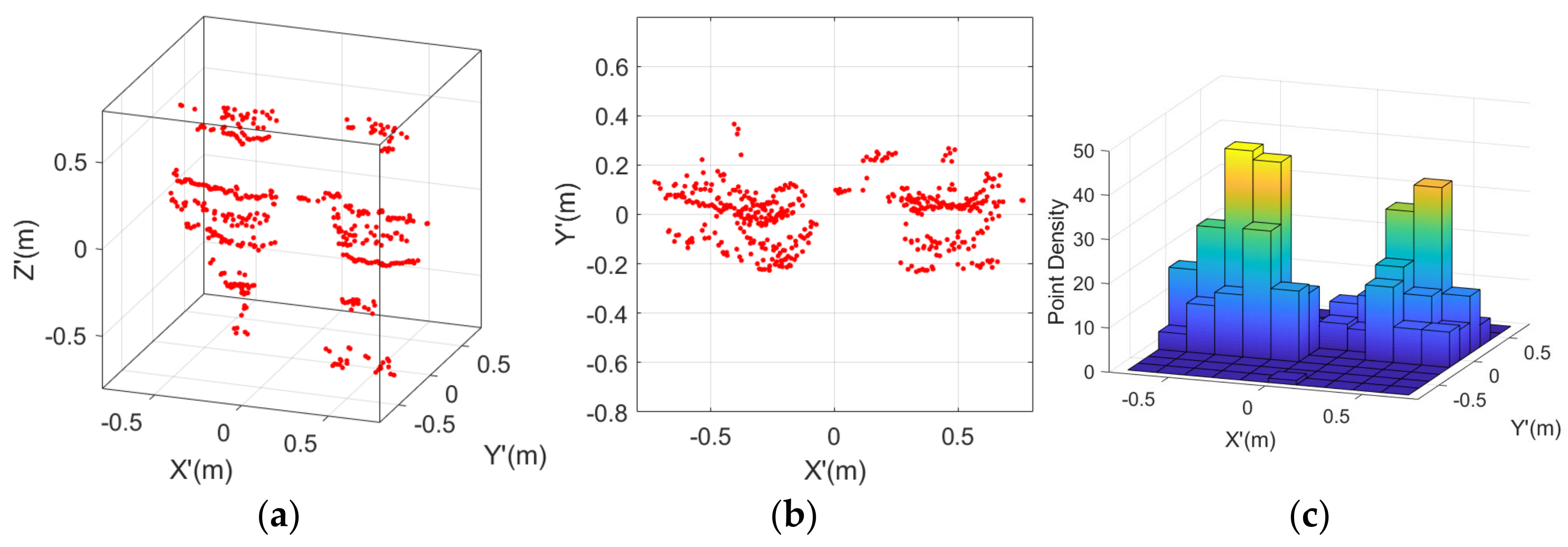
After the clustering process, every cluster is transformed into a local coordinate system to identify its geometric characteristics. For each cluster, the coordinates of all the points are first normalized by shifting to its centroid. Generally, pedestrians in urban scenarios remain upright, which is the direction of $z$-axis. As such, ${\left(0,0,1\right)}^T$ is defined as the $z^{\prime }$-axis of the local coordinate system. Then, a principal component analysis (PCA) is implemented to the $xy$ plane of this cluster, and the first and second principal components are defined as the $x^{\prime }$-axis and $y^{\prime }$-axis, respectively. Then point $\left(0,0,0\right)$ is defined as the origin $o^{\prime }$ of the local coordinate system, and the plane $o^{\prime }{x}^{\prime }{z}^{\prime }$ is defined as the main plane of the cluster. Similarly, planes $o^{\prime }{y}^{\prime }{z}^{\prime }$ and $o^{\prime }{x}^{\prime }{y}^{\prime }$ are defined as the secondary plane and the tertiary plane. A sample of the segmented pedestrian in its local coordinate system is shown in Figure 3, where Figure 3a is the 3D point cloud and Figure 3b–d are the projection results in the three planes. Based on these projected images, the size of the cluster can be defined by the following equations:

$$\left\{\begin{array}{c}l=x_{max}^{,}-x_{min}^{,}\\ w=y_{max}^{,}-y_{min}^{,}\\ h=z_{max}^{,}-z_{min}^{,}\end{array}\right.$$

(2)

where $l$,$w$, and $h$ are the length, width and height of the cluster, respectively. Then, all clusters are divided into three categories on the basis of their size: single pedestrian candidates, multiple pedestrian candidates, and non-pedestrians. Candidates of multiple pedestrians are segmented further in the following step.

3.2.3. Multiple Pedestrians’ Separation

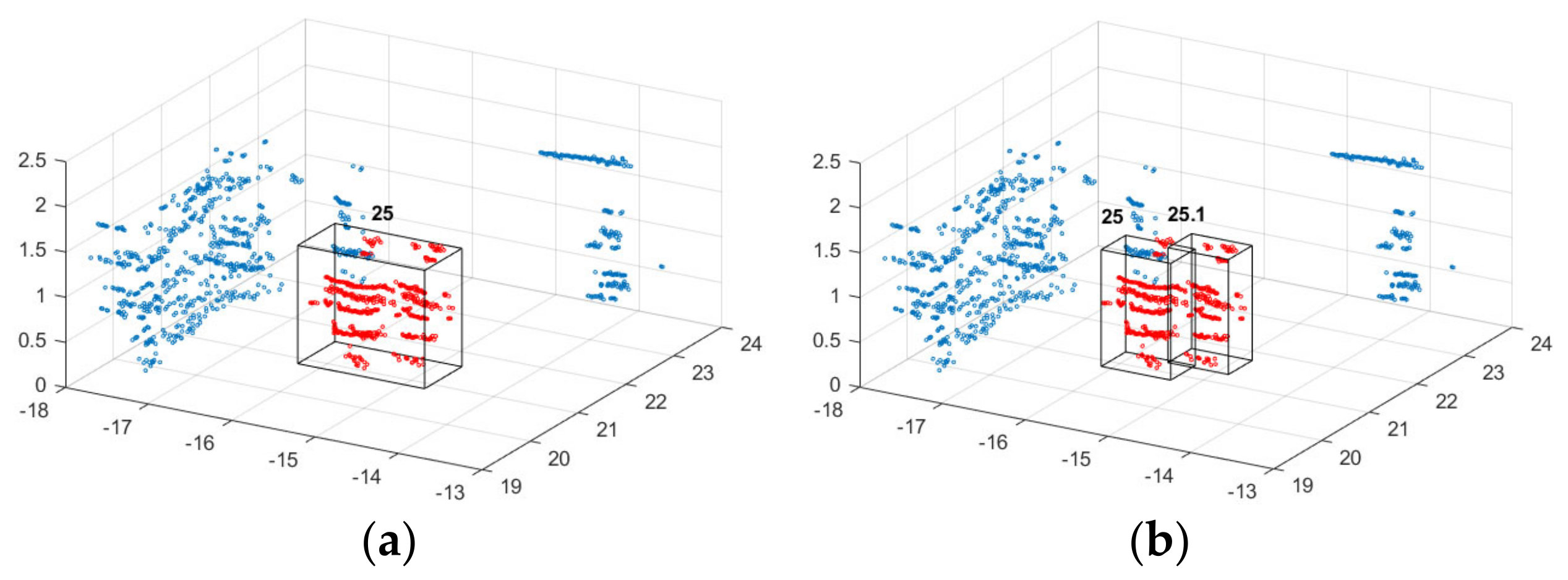
To separate the single pedestrian candidate from multiple pedestrian candidates, the mean shift algorithm was used [44]. The mean shift algorithm kept moving the centroid to the higher density region until the centroid reached a position from which it cannot move further. Although this clustering algorithm suffers from speed in large frames of point-cloud data [45], it works well for locating the density peaks of a density function. Generally, multiple pedestrian candidates contain two or three pedestrians that are close to each other, so it is not easy to separate them by a distance-based clustering algorithm in 3D space. For example, as can be seen in Figure 4a, the distance between the two pedestrians is less than the set radius $\epsilon$, so they are regarded as one cluster. However, as clearly shown in the projected image in the tertiary plane (Figure 4b), these two pedestrians correspond to the two maxima of the density function (Figure 4c). Therefore, it is feasible to separate multiple pedestrians by recognizing the number of regions with high point densities.

3.3. Pedestrian Classification

This step aims to extract features from pedestrian candidates and then classify them by pedestrian classifiers.

3.3.1. Feature Selection

Most of the previous studies [11,16,17,18] only use static features to represent pedestrians. However, the speed information is more straightforward for pedestrian detection, as the speed of a pedestrian is unique, compared to the static background and other moving objects. However, pedestrian detection with only speed information may fail in some cases. For example, if a pedestrian is static, their average radial velocity would always be zero; another scenario may be that the moving direction of a pedestrian is almost perpendicular to the laser beam in which the Doppler LiDAR cannot detect the velocity. Therefore, it is necessary to utilize both speed information and static features to achieve better pedestrian detection performance. In this study, a static feature vector composed of 28 features was calculated to describe a pedestrian. The descriptions and dimensions of the proposed features are listed in

Table 1. Features of a cluster for pedestrian classification.

Features	Description	Dimension
$f_1$	Number of points in the cluster	1
$f_2$	Average range of points to the sensor	1
$f_3-f_8$	Covariance matrix (3D) of the points in the cluster	6
$f_9-f_{14}$	Normalized moments of inertia tensor	6
$f_{15}-f_{26}$	Slice feature for the cluster	12
$f_{27}-f_{28}$	Mean and standard deviation of the intensities	2

. Features $f_1$–$f_{14}$ are introduced in [15]. Feature $f_1$ is the number points of a candidate cluster and $f_2$ is the range between this cluster and the sensor. Features $f_3$–$f_8$ and $f_9$–$f_{14}$ are the covariance matrix and normalized moments of inertia tensor of the points in the cluster, representing the overall distribution of points. Features $f_{15}$–$f_{28}$ are first proposed by [16]. Features $f_{15}$–$f_{26}$, named the slice feature, could depict the rough profile of a cluster and features $f_{27}–f_{28}$ are the mean and standard deviation of the intensities of points in a candidate cluster, which describe the reflectance characteristics of this pedestrian candidate.

Two different strategies were adopted to utilize the speed information. The first strategy generates a simple speed classifier based on the average radial velocity $v_r$ of the candidate clusters. The speed classifier discriminates the pedestrian candidates in the test data sets based on their speed information; all the pedestrian candidates whose average radial velocity satisfies a pre-defined velocity threshold $v_T$ are classified as pedestrians. Then, a machine learning-based classifier trained by the static features is utilized to classify the remaining clusters. The other strategy is to count $v_r$ as $f_{29}$ and merge it with other features to form a 29-dimensional feature vector. Then, the machine learning-based classifier trained by this feature vector is utilized to classify the pedestrian candidates in the test data sets.

3.3.2. Classification Method

In this study, the performance for the pedestrian detection of two different machine learning algorithms (MLAs) is evaluated: SVM and random forest (RF) [46]. These two MLAs were selected for the following reasons: (1) they are easy to implement and able to reproduce the results, as they are found in most machine learning algorithm libraries, and (2) many previous studies related to 3D LiDAR-based object classification were implemented by them and have shown good performance [47,48,49].

3.3.3. Evaluation Metrics

There are several metrics that can be used to evaluate the performance of the pedestrian classifiers. These metrics can be calculated based on the confusion matrix, which presents the number of samples that are correctly classified by a machine learning algorithm (true positives (TP) and true negatives (TN)) against those which are not (false positives (FP) and false negatives (FN)). As pedestrian detection requires a binary classifier, several metrics can be calculated from the confusion matrix, such as precision, recall and the F1-score. Specifically, precision is the predictive power of the algorithm to evaluate its effectiveness in detecting a single class. It can be expressed as follows:

$$\mathrm{Precision}=\frac{\mathrm{TP}}{\mathrm{TP}+\mathrm{FP}}$$

(3)

Recall evaluates the effectiveness of the algorithm in detecting a single class and can be expressed as follows:

$$\mathrm{Recall}=\frac{\mathrm{TP}}{\mathrm{TP}+\mathrm{FN}}$$

(4)

The F1-score is the harmonic mean of precision and recall and can be expressed as follows:

$$\mathrm{F}1–\mathrm{score}=\frac{2\times \mathrm{Precision}\times \mathrm{Recall}}{\mathrm{Precision}+\mathrm{Recall}}$$

(5)

3.4. Pedestrian Tracking

This step aims to associate detected pedestrians in the current frame with the existed tracks from the previous frame and then update the tracks.

3.4.1. State Prediction

After detection, the next step is to track the detected pedestrians. The proposed pedestrian tracking algorithm is built on a Kalman filter [50]. A Kalman filter is a probabilistic inference model that makes optimal estimation of the state of a system from predictions and measurements. It produces values closer to the real values by analyzing the uncertainty of the predictions and measurements.

In the detection step, one assumption is that pedestrians in urban scenarios remain upright, so pedestrians move in the $xy$ plane. Thus, the state vector $\mu$ of a detected pedestrian in frame $k-1$ consists of eight parameters:

$$\mu ={(x,y,l,w,h,\theta ,v_x,v_y)}^T$$

(6)

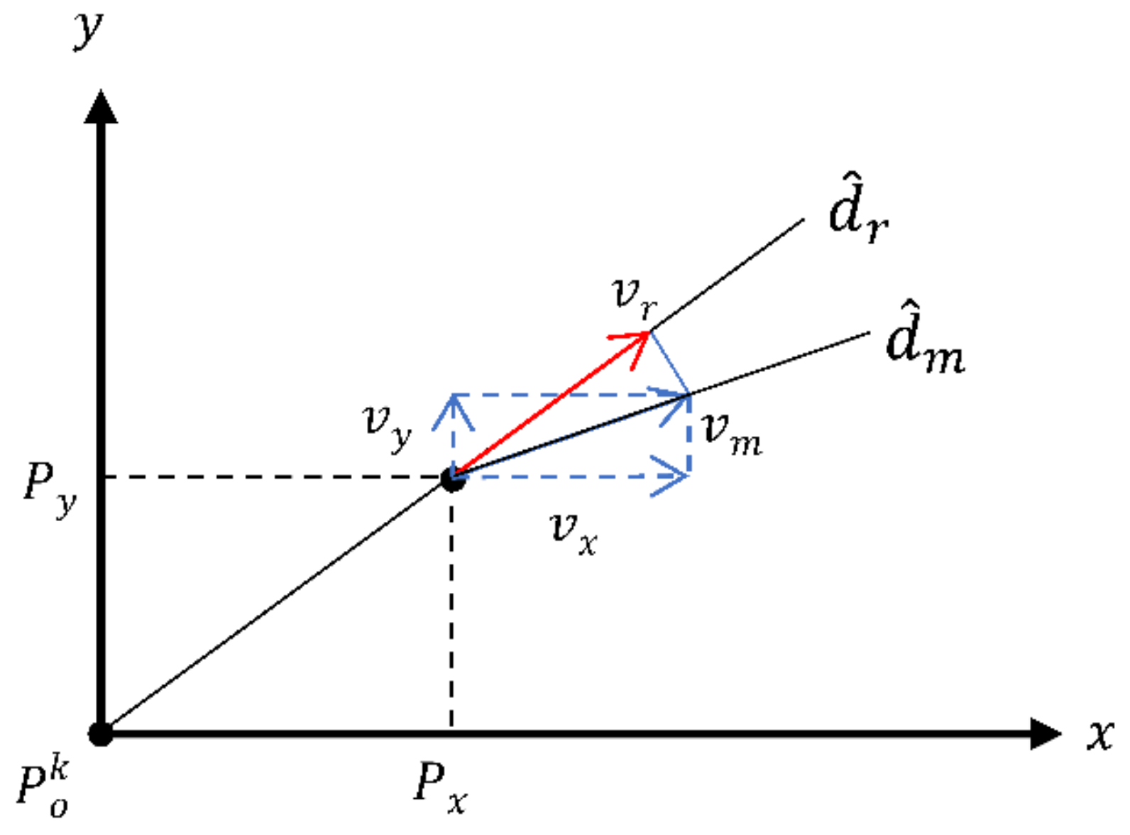
where $\left(x,y\right)$ are the $xy$ coordinates of a pedestrian’s position; $\left(l,w,h\right)$ represent the width, length, and height of the pedestrian, respectively; $\theta$ is the pedestrian orienation about the z’-axis; $\left(v_x,v_y\right)$ represent the velocity of the pedestrian in the $xy$ direction. In detail, given the scanner position $P_o^k,$ and the pedestrian’s moving direction, ${\widehat{d}}_m$, $v_x$ and $v_y$ can be estimated from the measured radial velocity $v_r$. As shown in Figure 5, for a given detection $D_i^k$ at $P_i^k$, the vector of beam direction can be expressed as follows:

$${\widehat{d}}_r=P_i^k-P_o^k$$

(7)

Thus, the total speed $\Vert v_m\Vert$ of a pedestrian can be formulated as follows:

$$\parallel v_m\Vert {}_{ }=\frac{\parallel {\widehat{d}}_m\Vert \Vert {\widehat{d}}_r\parallel }{{\widehat{d}}_m·{\widehat{d}}_r}\Vert v_r\parallel$$

(8)

To model the dynamics of pedestrians, a constant velocity model is adopted as the process model, which defines the propagation of the state from the previous frame to the current frame. All the associated trajectories $T^{k-1}$ from frame $k-1$ are propagated to frame $k$ by the following equation:

$$\begin{gathered} x^k=x^{k-1}+v_x^{k-1}\Delta t+u_x \\ {y}^k=y^{k-1}+v_y^{k-1}\Delta t+u_y \end{gathered}$$

(9)

where $\left(u_x,u_y\right)$ are the process noise in this model, and $\Delta t$ is the time interval between two adjacent frames (0.2 s in this study). Additionally, the dimensions and orientation of a pedestrian are assumed to be constant, so they do not change during the prediction step. Then, the Kalman filter prediction step is formulated in matrix form as follows:

$${\overline{\mu }}^k=F{\mu }^{k-1}$$

(10)

$${\overline{\Sigma }}^k=F{\Sigma }^{k-1}{F}^T+Q$$

(11)

where ${\mu }^{k-1}$ and ${\Sigma }^{k-1}$ are the state vector and its covariance matrix at frame $k-1$; ${\overline{\mu }}^k$ and ${\overline{\Sigma }}^k$ are the predicted state and the covariance matrix at frame $k$; $F$ is the state transition matrix; and $Q$ is the covariance matrix of the process noise.

3.4.2. Detection-to-Track Association

For each detected pedestrian at frame $k$, the sensor can provide its position and velocity, so the measurement model is as follows:

$${\overline{z}}^k=H{\overline{\mu }}^k$$

(12)

$$S^k=H{\overline{\Sigma }}^k{H}^T+R$$

(13)

where ${\overline{Z}}^k$ and $S^k$ are the predicted measurement and its innovative matrix; $H$ is the measurement matrix; and $R$ is the covariance matrix of the measurement noise.

To associate the detected pedestrians at frame $k$ with the existed tracks from frame $k-1$, the Mahalanobis distance [51] is adopted to measure their similarity. The Mahalanobis distance between the predicted detection ${\overline{z}}_i^k$ and the actual detection $z_j^k$ is formulated by the following equation:

$$d_m^k\left(i,j\right)=\sqrt{{\left(z_j^k-{\overline{z}}_i^k\right)}^T {\left(S_i^k\right)}^{-1}{\left(z_j^k-{\overline{z}}_i^k\right)}^{ }}$$

(14)

where $d_m^k\left(i,j\right)$ is the Mahalanobis distance between the predicted detection $i$ and the measured detection $j$. Given the Mahalanobis distance between each pair of predictions and detections, a greedy algorithm [33] is used to match the detections and trajectories.

3.4.3. State Update

After the detection-to-track association step, an initialization and termination module is used to initialize new tracks for the unmatched detections and to eliminate unmatched tracks. To avoid false positive tracks, a new track is not created for an unmatched pedestrian until it is detected in three consecutive frames. The state vector of a new track is calculated according to its most recent detection. Similarly, to avoid terminating the true tracks, which miss detections at some frames, each track is not deleted until it cannot be matched with any detections in three consecutive frames. During this process, the state vector of the unmatched pedestrians is also updated with its last known velocity estimation by the process model. The tracks with missing detections are recovered by this strategy and only the tracks that leave the scene are terminated.

For matched pairs of detections and predictions, their predicted state mean and covariance matrix are updated by the following equations:

$${\Sigma }^k={\overline{\Sigma }}^k\left(I-K^k{H}^{ }\right)$$

(15)

$${\mu }^k={\overline{\mu }}^k+K^k\left(z^k-{\overline{z}}_{ }^k\right)$$

(16)

where $K^k$ is the optimal Kalman gain, which can be calculated by the following:

$$K^k={\overline{\Sigma }}^k{H}^T{\left(R+H{\overline{\Sigma }}^k{H}^T\right)}^{-1}$$

(17)

3.4.4. Evaluation Metrics

There are several metrics that can be used to evaluate the performance of the proposed tracking approach: FP, FN, identity switch (IDSW), and MOTA. A pedestrian that is missed by any hypothesis is a FN, and a non-pedestrian that is wrongly assigned to a track is a FP. An IDSW is counted if a ground truth target $\mathrm{i}$ is matched to an incorrect track $\mathrm{j}$. MOTA is used to evaluate a tracker’s overall performance by combining all the above sources of errors and can be expressed as follows:

$$\mathrm{MOTA}=1-\frac{{\sum }_{\mathrm{K}}\left({\mathrm{FN}}_{\mathrm{k}}+{\mathrm{FP}}_{\mathrm{k}}+{\mathrm{IDSW}}_{\mathrm{k}}\right)}{{\sum }_{\mathrm{k}}{\mathrm{GT}}_{\mathrm{k}}}$$

(18)

where $\mathrm{k}$ is the frame index and $\mathrm{GT}$ is the number of ground truths.

4. Results

This section presents the results of the proposed pedestrian detection and tracking with the collected two data sets. The performance of the pedestrian detection is evaluated by the recall, precision and F1-score. Additionally, this section shows that the performance of pedestrian classification is clearly varied by the distance to the target. The results of the pedestrian tracking are presented as well, while its performance is evaluated by a set of tracking quality measures.

4.1. Pedestrian Detection

This session shows the qualitative and quantitative results of pedestrian detection, then discusses the effect of the speed information in detail.

4.1.1. Cluster Detection

The objective of cluster detection is to find all the clusters likely to be pedestrians. Therefore, the pedestrian candidates should contain ground truth as much as possible since only the clusters extracted from the clustering algorithm would be regarded as pedestrian candidates and then be classified by the classier. The size thresholds for potential single pedestrian candidates are as follows:

$$C_p=\left\{C_i|0.6m<h_i<2m , 0.2m<l_i<1.2m ,0.15m<w_i<0.8m\right\}$$

where $C_p$ is the set of pedestrian candidates. The above criteria are determined according to the height, shoulder width and step length of the pedestrians. Based on these values, the size thresholds for potential multiple (usually two or three) pedestrians’ candidates are as follows:

$$C_{mp}=\left\{C_i|0.6m<h_i<2m ,1.2m<l_i<3m ,0.8m<w_i<3m\right\}$$

where $C_{mp}$ is the set of multiple pedestrian candidates.

In the multiple pedestrian separation process, the multiple pedestrian candidates are segmented into single pedestrian candidates successfully. As Figure 6a shows, two pedestrians very close to each other are far from the scanner. Therefore, a relatively large $\epsilon$ value is assigned to them during the clustering process, so they are clustered as one object. In the next step, the mean shift-based separation process (Figure 6b) is applied to further separate them.

Recall, which is the ratio between the number of pedestrians extracted by the clustering process and the ground truth, is adopted to quantitatively evaluate the performance of the proposed cluster detection algorithm. As shown in

Table 2. Performance of pedestrian candidate detection (#: count of pedestrians).

Data Set	#Frames	#Ground Truth of Pedestrians	#Pedestrians	#Missing Pedestrians	Recall
I	90	1602	1362	240	0.8496
II	107	1327	974	353	0.7340

, for Data Set I, the recall is about 85%, which indicates that 15% of the pedestrians are not extracted during the process of cluster detection; the recall of Data Set II is only 73%. Different major directions of pedestrian flow in the scenes are the main cause for the varying performance of the clustering method. In Data Set I, where our vehicle stopped at a traffic light, most of the pedestrians were crossing the street. Although their radial velocity would be insignificant when they pass in front of the Doppler LiDAR, they were fully scanned and had a complete shape. In contrast, for Data Set II, where our vehicle was moving, most of the pedestrians were walking along the street as well. The radial velocity of the moving pedestrians was significant in this condition, but some of the pedestrians were only partially scanned because they were obstructed by others or objects, such as vehicles and poles, which resulted in a relatively low recall.

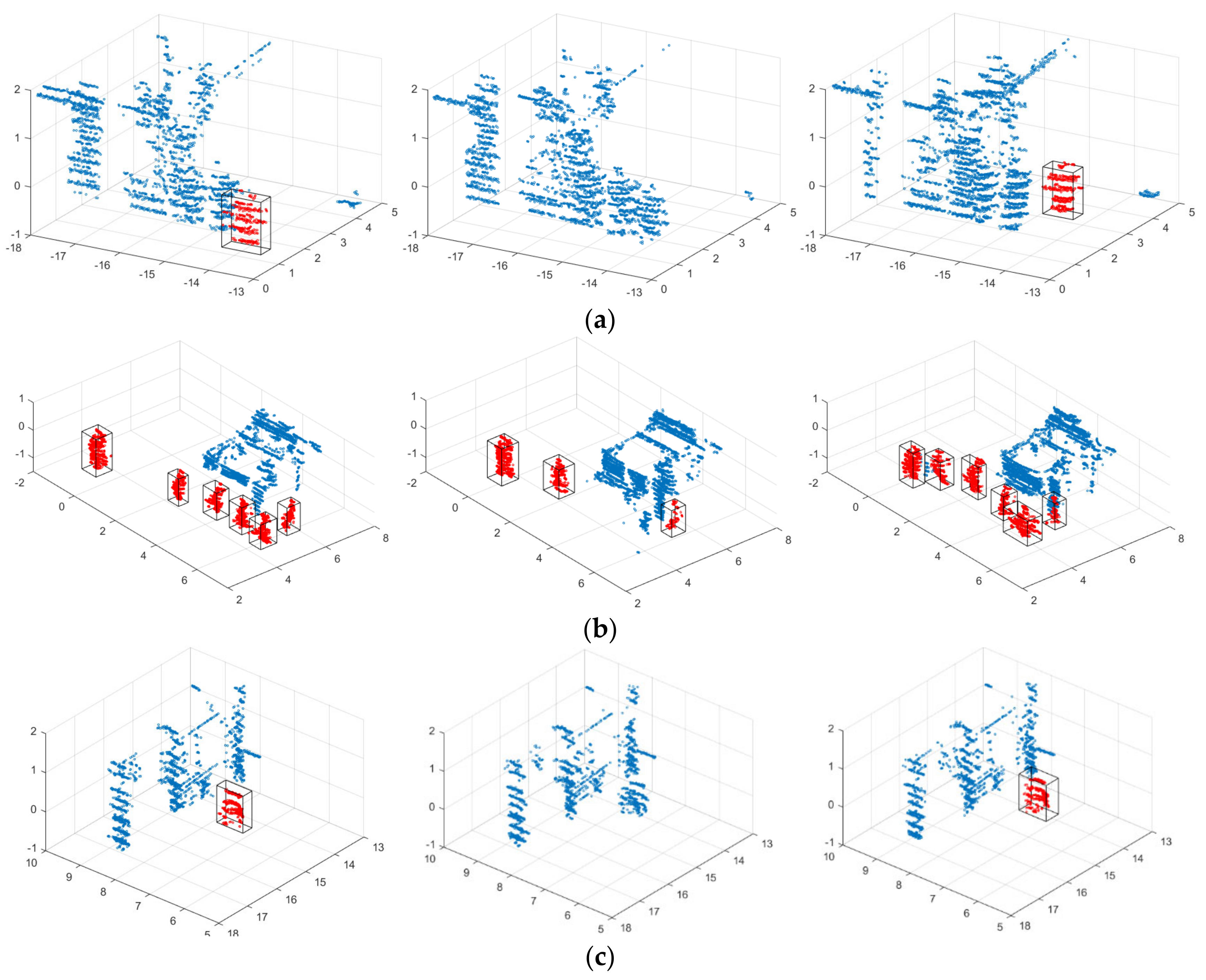
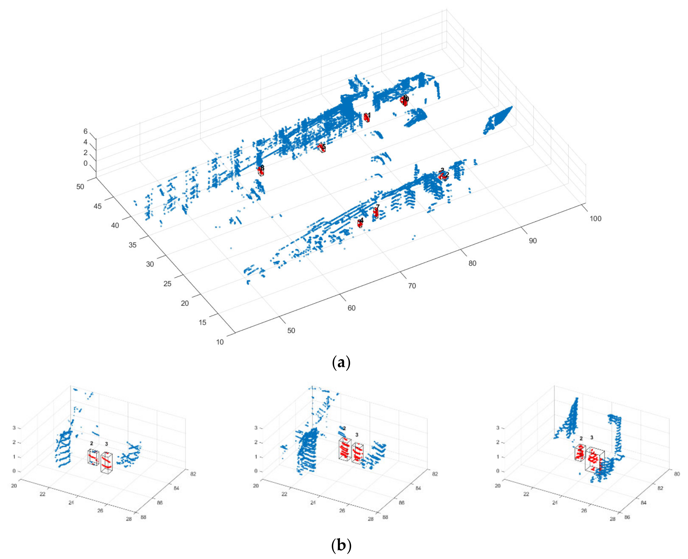
Missing detections, or FNs, are produced by various causes (

Table 3. Summary of missing pedestrians (#: count of pedestrians).

Data Set	#Unsegmented Pedestrians	#Partially Scanned Pedestrians	#Mismatched Pedestrians
I	18	201	21
II	37	294	22

). To be specific, missing detections can occur in either the clustering or selection of pedestrian candidate processes. In the clustering process, if pedestrians are too close to large objects (e.g., buildings), they may not be segmented as a single pedestrian. Instead, they can be regarded as a part of the large objects. For example, as shown in Figure 7a, a pedestrian was passing by a building in three frames. In the first and last frame, the distance between the pedestrian and the building is larger than $\epsilon$, so this pedestrian is segmented to a single cluster and selected as a pedestrian candidate in the following step. However, in the second frame, this distance becomes less than $\epsilon$, so the pedestrian is merged into the cluster of the building. In addition, unlike clusters composed of multiple pedestrians, the size of such a cluster is much larger than the threshold set for multiple pedestrian candidates; as a result, this pedestrian is not successfully extracted by the multiple pedestrian separation process.

In the selection of pedestrian candidates process, both the partially scanned point clouds and the unmatched sizes lead to missing detections. As shown in Table 3, over 80% FNs are produced, due to partially scanned point clouds. An example of partially scanned point clouds is shown in Figure 7b, where there are six detected pedestrians in the first and last frames. However, in the second frame, the point clouds of three pedestrians are only partially collected by the sensor, so they are not detected in the selection of pedestrian candidates step because their sizes are smaller than the thresholds set previously. In Data Set II, some pedestrians are constantly occluded by other objects, so they are not detected in most frames. A more extreme case is a pedestrian who completely disappears in one or more frames. Missing detections also happen when one or more size of a cluster are not in the range of the predefined threshold. As shown in Figure 7c, a pedestrian is detected successfully in the first and last frames but is missed in the second frame because their height is smaller than the threshold.

4.1.2. Pedestrian Classifier

To train the supervised machine learning-based classifiers, for each data set, 60 percent of the samples were used as training data and 40 percent of the samples were used as testing data. The descriptions of the two data sets are shown in

Table 4. Summary of training and testing data for pedestrian classification (#: count).

Data Set	Description	#Positive Samples	#Negative Samples	Total
I	Training data	882	2824	3706
	Testing data	480	1662	2142
II	Training data	650	1906	2556
	Testing data	324	1162	1486

.

The proposed two-step classifier is composed of a speed classifier and a machine learning-based classifier. According to the specifications of the Doppler LiDAR [41], the precision of the radial velocity is $0.1\mathrm{m}/\mathrm{s}$, so we set the lower bound of $v_r$ as 0.3$\mathrm{m}/\mathrm{s}$, which is strict enough to filter out most static objects. The upper bound of the $v_T$ is set as $2\mathrm{m}/\mathrm{s}$ because, generally, a pedestrian is not likely to move faster than that. The quantitative results for each step are shown in

Table 5. Quantitative results of each stage of the two-step classifier.

Data Set	MLA	Stage	TP	FP	FN	TN
I	SVM	I	460	11	20	1651
		II	465	39	15	1623
	RF	I	460	11	20	1651
		II	471	18	9	1644
II	SVM	I	288	31	35	1131
		II	307	81	16	1079
	RF	I	288	31	35	1131
		II	310	52	14	1110

. After the speed classifier (stage I), the static objects are removed since their average radial velocities are not likely to be larger than the $v_T$. Generally, FPs are over-segmented vehicles and pedestrians. As previously mentioned, the FNs are pedestrians with insignificant radial velocity. The remaining clusters are then input to the machine learning-based classifier (stage II). The results show that the FNs decrease because the pedestrians misclassified in stage I are classified correctly in stage II by the SVM or RF classifier. In contrast, the FPs increase because some of the non-pedestrians are classified as pedestrians incorrectly during this process.

Unlike SVM, it is unnecessary to project the features in RF to a higher dimension space by the kernel trick to find the optimal separable hyperplane. Therefore, the importance of the features can be ranked, according to the GINI index. The importance of features for the RF classifier are shown in Figure 8. The average radial velocity of a cluster $\left(f_{29}\right)$ is the most important feature among all the features. Therefore, it is reasonable to use $f_{29}$ as the only feature to form the speed classifier.

To evaluate the effect of the speed classifier as well as the effect of the speed information, we compare the results from two two-step classifiers (named two-step SVM and two-step RF), two one-step classifiers with the speed information (named SVM-Speed and RF-Speed) and two one-step classifiers without the speed information (named SVM and RF). As can be seen from

Table 6. Quantitative results of different pedestrian classifiers.

Classifier	Data Set	Precision	Recall	F1-Score
Two-step-SVM	I	0.9226	0.9688	0.9451
	II	0.7877	0.9506	0.8615
SVM-Speed	I	0.9703	0.9542	0.9622
	II	0.8837	0.8210	0.8512
SVM	I	0.8816	0.7292	0.7982
	II	0.7689	0.6265	0.6905
Two-step RF	I	0.9632	0.9812	0.9721
	II	0.8410	0.9568	0.8947
RF-Speed	I	0.9651	0.9792	0.9721
	II	0.8909	0.9074	0.8991
RF	I	0.9002	0.8083	0.8518
	II	0.7994	0.7554	0.7767

, all six classifiers perform better on the Data Set I, where the LiDAR vehicle stopped. The performance differences can also be explained by the different major direction of pedestrian flow in the scenes. To be specific, pedestrians crossing the street were more likely to be classified correctly since their fully scanned point clouds could provide better geometry features.

Overall, classifiers with the speed information outperform classifiers without the speed information on all the evaluation metrics, especially the recall. The F1-scores among four classifiers with speed information are not significantly different. For SVM-based classifiers, the two-step SVM has higher recall, and the SVM-speed has higher precision. This is because SVM-speed recognizes pedestrians based on both the speed information and the static features, so some of the pedestrians with very blurred contours are misclassified, even if they are moving. In contrast, the speed classifier is able to recognize moving pedestrians only by their average radial velocity and, therefore, is able to detect all of the moving pedestrians. For RF-based classifiers, the two-step RF and the RF-speed show similar performance. A possible explanation is that once the subset of features is selected by an individual tree, including the average radial velocity, the role of this feature is similar to a simple speed classifier. For the classifiers based on different MLAs, it is concluded that the overall performance of the RF-based classifiers outperforms the SVM-based classifiers. In detail, the average F1-score of SVM-based and RF-based classifiers are 0.8515 and 0.8944, respectively. Therefore, the detection results from two-step RF can be used to track pedestrians.

The detection results of the classifiers in varied ranges are listed in

Table 7. Quality of pedestrian detection at the different ranges from the sensor.

		<30 m			30–60 m
Classifier	Data Set	Precision	Recall	F1-Score	Precision	Recall	F1-Score
Two-step-SVM	I	0.9245	0.9423	0.9333	0.9317	1.000	0.9647
	II	0.8415	0.9695	0.9011	0.6023	0.7689	0.7114
SVM-Speed	I	0.9692	0.9087	0.9380	0.9703	0.9542	0.9622
	II	0.9000	0.8212	0.8727	0.6712	0.8033	0.7313
SVM	I	0.9180	0.8077	0.8593	0.8989	0.6854	0.7777
	II	0.7879	0.6920	0.7368	0.6363	0.3443	0.4468
Two-step RF	I	0.9803	0.9567	0.9684	0.9512	1.000	0.9750
	II	0.8900	0.9811	0.9382	0.6500	0.8526	0.7376
RF-Speed	I	0.9754	0.9519	0.9635	0.9579	1.000	0.9785
	II	0.9461	0.9354	0.9407	0.6857	0.7869	0.7328
RF	I	0.9178	0.9135	0.9157	0.8844	0.7289	0.7992
	II	0.8132	0.8377	0.8253	0.6944	0.4032	0.5102

. As the distance between the objects and the sensors increase, the overall performance of most of the classifiers declines, indicating a decreasing trend for pedestrian detection efficiency. However, the four classifiers with speed information generally perform better than the classifiers having only static features, especially for pedestrian detection at ranges larger than 30 m. For close pedestrian detection, static features are sufficient to detect most pedestrians, and additional speed information improves both the recall and F1-score by 10%, respectively. Based on these outcomes, it is concluded that both static features and speed information are important to detect pedestrians at the range of 30 m. However, most static features are sensitive to spatial resolution of the point clouds. When the distance increases, the number of points are returned as the pedestrians decrease, so the contour of the candidate pedestrians gradually blurs or is even lost, which makes the shapes less different between pedestrians and other objects. Unlike static features, the speed information is not distance dependent. Therefore, as the distance increases, its performance is still much better than classifiers only with static features, although the performance of the two-step classifiers and one-step classifier with speed decreases. In Data Set I, the additional speed information improves the F1-score by 20%. In Data Set II, the two classifiers with only static features completely fail to detect pedestrians in this region because most of the pedestrians that are at the range of 30 m to 60 m do not have a clear shape, whereas the two-step classifier and the one-step classifier with speed information are still able to classify the pedestrians. Therefore, it is concluded that speed information plays a crucial role in detecting pedestrians, especially when they are far away from the sensor.

In summary, during the clustering process, the proposed method is able to separate a single pedestrian well. In the pedestrian classification, the average radial velocity improves the classification performance significantly, especially for pedestrians at the range of 30 m to 60 m to the sensor. The performance of RF is slightly better than the SVM. Overall, the highest recall (0.9812 and 0.9568 for Data Sets I and II, respectively) is obtained by adopting the proposed two-step classifiers, which use speed information to extract most moving pedestrians, while the highest precision (0.9703 and 0.8909) for Data Set I and II respectively) is obtained by adopting the one-step classifiers with the speed information. For the purpose of pedestrian tracking, a higher recall is more important than precision. As a non-pedestrian may not be misclassified as a pedestrian in all consecutive frames, its influence could be eliminated by an appropriate tracking management strategy. In contrast, pedestrians with only a sparse or partially scanned point cloud are likely to be missed in the pedestrian classification step, which will result in increasing tracking errors.

4.2. Pedestrian Tracking

The results with and without speed measurements in the proposed tracking algorithm are shown in

Table 8. Quality of Kalman filter tracking with and without speed information.

Data Set	Method	FN	FP	IDSW	MOTA
I	KF-Speed	75	1	7	0.8391
	KF	82	1	11	0.8178
II	KF-Speed	199	7	4	0.5527
	KF	204	7	4	0.5445

. It is obvious that the tracking quality of Data Set I is better because the detection quality is crucial to the tracking system. In general, pedestrians that are not constantly detected are not likely to be tracked well because the disappearance of them in some frames would lead to FNs or IDSW. Most FNs are undetected pedestrians, while others are produced during the classification and tracking process. Due to the strategy for new tracks generation, the FPs are quite low for both data sets since most of them do not occur constantly, so no new tracks would be created for them. Compared to the original Kalman filter (KF), the Kalman filter with the speed information (KF-Speed) is less likely to have errors, but their difference is small. A possible explanation is that the speed of most pedestrians does not change significantly, so even the KF without speed information is able to track well detected pedestrians.

Some sample results of pedestrian tracking are shown in Figure 9a. The red clusters represent pedestrians, and the blue points are the static background and other objects. The black boxes represent the 3D bounding box of each tracked pedestrian, and the corresponding number is the unique tracking ID of each pedestrian.

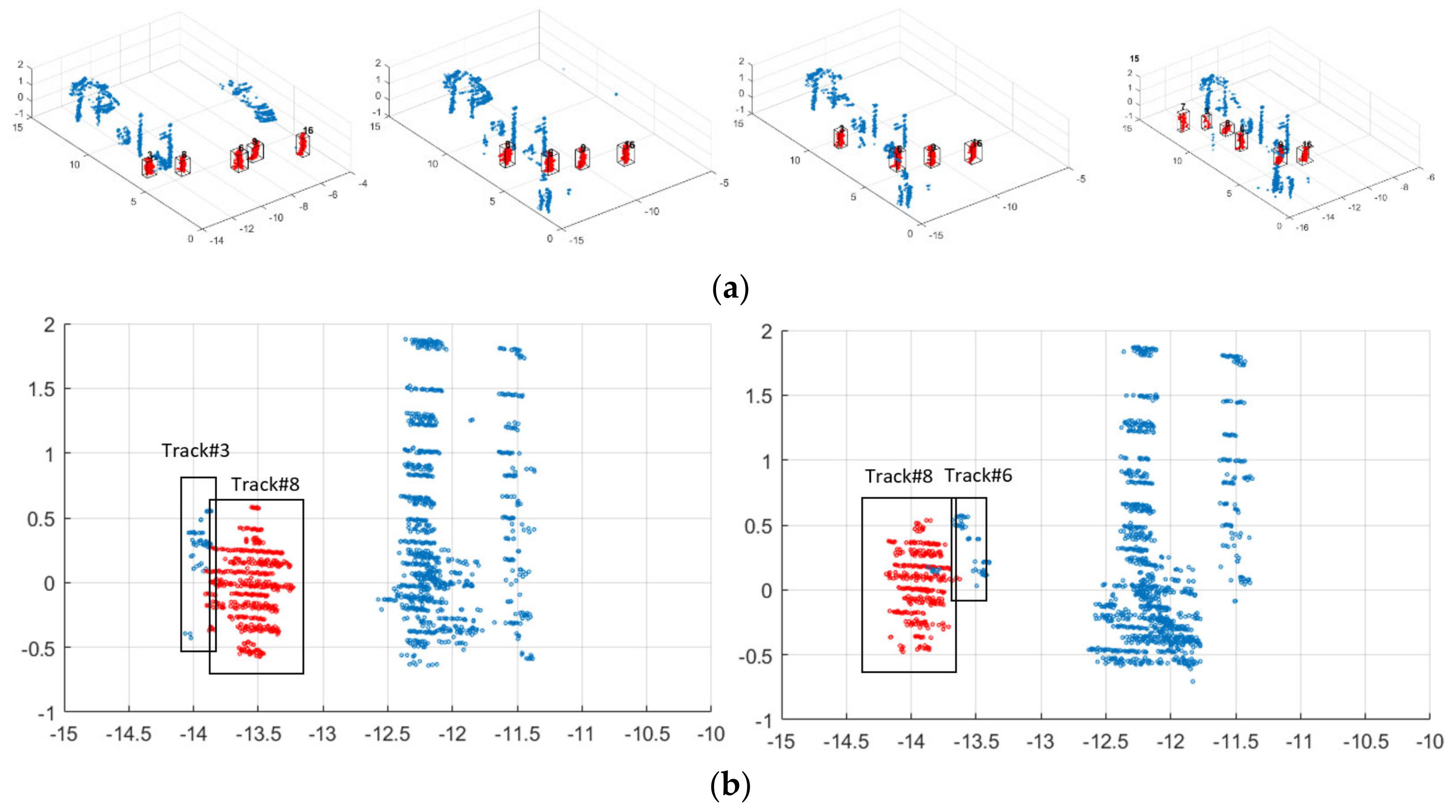
The results show that the proposed tracking method can track pedestrians on crowded streets. For example, in Figure 9b, two pedestrians are tracked completely over ten frames until they leave the scene. Additionally, the proposed strategy that manages the initialization and termination of the trajectories is able to deal with the FNs generated during the detection step. For example, in Figure 10a, three close pedestrians are walking along the street (tracked as #1, #2 and #14). In frame 70 (Figure 10b), the pedestrian corresponding to Track #1 is classified incorrectly. Thus, in the data association step, Track #1 is not associated with any detected pedestrians, but it is not terminated immediately. Instead, its state vector is updated and propagated to the next frame by using its current velocity, so it can still be tracked by the same track ID in future frames (Figure 10c). However, the pedestrian that belongs to Track #14 is missed in three consecutive frames (frames 74 to 76), so Track #14 is terminated, and Track #20 is initialized for this pedestrian (Figure 10d). As shown in Figure 11a, five pedestrians are fully tracked in frames 64 through 82. However, in frames 72 and 74, Track #3 and Track #8 are partially scanned so that those pedestrians could not be detected successfully (Figure 11b) and are recovered once their corresponding pedestrians are detected again.

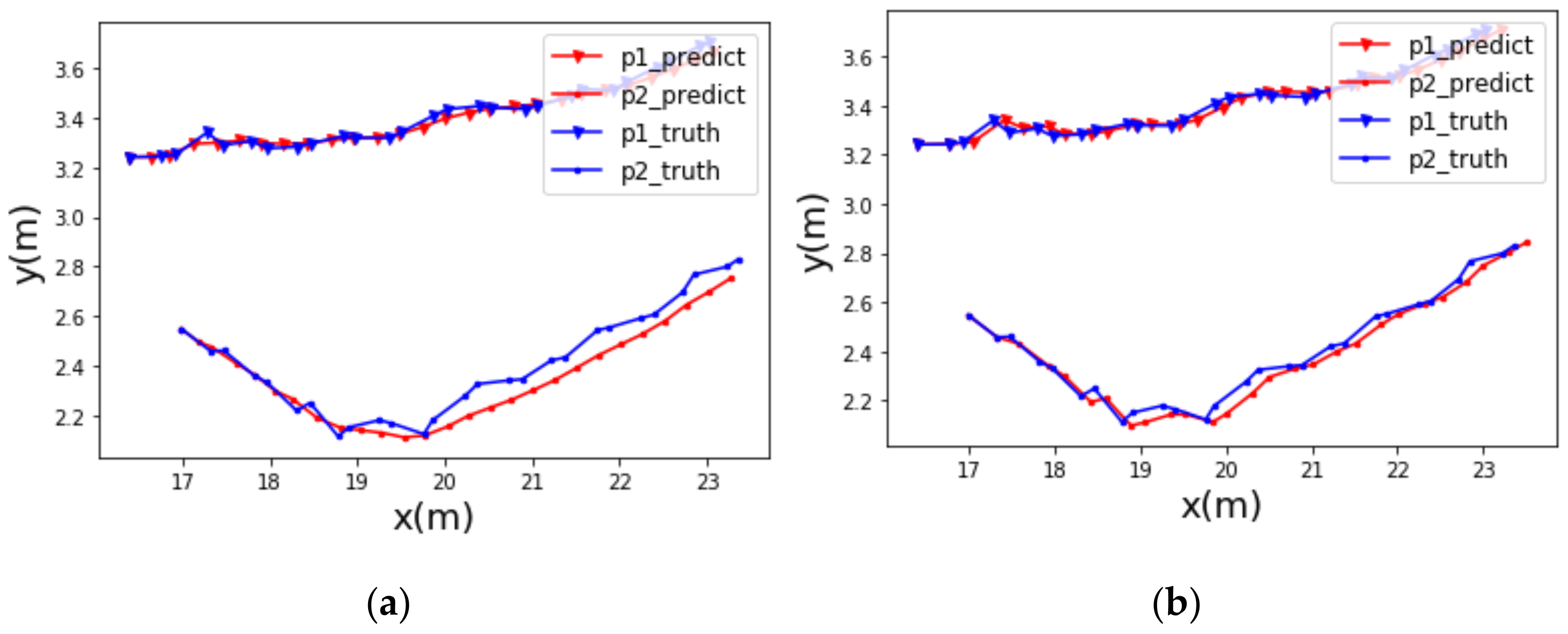
To evaluate the effect of speed information on position estimation, the trajectories of two close pedestrians are visualized in Figure 12. The red and blue points represent their predicted and true positions, respectively. It is obvious that, compared to the KF (Figure 12a), KF-Speed (Figure 12b) is able to provide more reliable predictions of the locations. The root means square error (RMSE) between the predicted locations and true locations is adopted to quantitatively evaluate the accuracy of the predicted location of these two KF models; the results are shown in

Table 9. RMSE between predicted locations and true locations.

Pedestrian	Method	RMSE (m)
p1 (Figure 12)	KF-Speed	0.113
	KF	0.145
p2 (Figure 12)	KF-Speed	0.137
	KF	0.180

. For these two pedestrians, the KF-Speed decreases the RSME by 0.032 and 0.043 m, respectively.

5. Discussion and Conclusions

The performance of the proposed approach was discussed in terms of both pedestrian detection and tracking. Pedestrian detection consisted of pedestrian candidate selection and pedestrian classification. The mean shift-based multiple pedestrian separation process, which was introduced between the clustering step and classification step, was shown to be capable of extracting single pedestrian candidates from multiple pedestrian candidates effectively (Figure 6). To evaluate the effect of the speed information in the classification, we compared the performance of the classifiers with the speed information to the performance of those without the speed information. In general, the classifiers including the speed information outperformed those without the speed information, especially for detecting pedestrians that were far from the scanner. With the speed information, missing detections only occurred when pedestrians fulfilled both of the following conditions: (1) pedestrians were occluded or far from the sensor, and (2) their average radial velocity was nearly zero. In addition, by utilizing the speed information, the average recall for the two data sets was 0.9399. Such a high recall is capable of improving the performance of pedestrian tracking. We also compared the performance of SVM-based classifiers and RF-based classifiers. Overall, the performance of the RF-based classifiers was better than the SVM-based classifiers no matter whether the speed information was included, so the detection result from the two-step RF was selected as input for pedestrian tracking since it achieves highest recall. In the tracking stage, the state vector of the pedestrians was estimated by using both position observations and speed observations, which increased the precision of the predicted movements of the pedestrians, thus improving the tracking quality.

There are several areas where the proposed method could be improved in future work. First, the detection method could only segment pedestrians that are close to other pedestrians or small objects, such as road signs. When pedestrians are moving close to large objects, such as buildings or poles, they are often regarded as a part of them. Future research could investigate a method of segmenting a pedestrian from a larger cluster. Second, there are some pedestrians missed because one or more of their dimensions are out of the range of the pre-defined thresholds. Therefore, more adaptive criteria should be proposed to include these pedestrians. Third, the proposed approach detects pedestrians frame by frame but does not consider their relationship between consecutive frames. For Data Set II, the proposed frame-by-frame clustering method missed about 25% of the pedestrians. However, the detection results from previous frames can definitely help in recognizing pedestrians in the current frame, especially for detecting partially scanned pedestrians. Lastly, even though the constant velocity model achieves high performance in pedestrian tracking, some more complex and advanced models, such as constant turn rate and velocity [52], could be investigated to improve the tracking performance.

References

1. Cao, X.-B.; Qiao, H.; Keane, J. A Low-Cost Pedestrian-Detection System with a Single Optical Camera. IEEE Trans. Intell. Transp. Syst. 2008, 9, 58–67. [Google Scholar] [CrossRef]
2. Stewart, R.; Andriluka, M. End-to-End People Detection in Crowded Scenes. arXiv 2015, arXiv:1506.04878. [Google Scholar]
3. Gaddigoudar, P.K.; Balihalli, T.R.; Ijantkar, S.S.; Iyer, N.C.; Maralappanavar, S. Pedestrian Detection and Tracking Using Particle Filtering. In Proceedings of the 2017 International Conference on Computing, Communication and Automation (ICCCA), Greater Noida, India, 5–6 May 2017; pp. 110–115. [Google Scholar]
4. Jafari, O.H.; Mitzel, D.; Leibe, B. Real-Time RGB-D Based People Detection and Tracking for Mobile Robots and Head-Worn Cameras. In Proceedings of the 2014 IEEE International Conference on Robotics and Automation (ICRA), Hong Kong, China, 31 May–7 June 2014; pp. 5636–5643. [Google Scholar]
5. Premebida, C.; Carreira, J.; Batista, J.; Nunes, U. Pedestrian Detection Combining RGB and Dense LIDAR Data. In Proceedings of the 2014 IEEE/RSJ International Conference on Intelligent Robots and Systems, Chicago, IL, USA, 14–18 September 2014; pp. 4112–4117. [Google Scholar]
6. Liu, J.; Liu, Y.; Zhang, G.; Zhu, P.; Chen, Y.Q. Detecting and Tracking People in Real Time with RGB-D Camera. Pattern Recognit. Lett. 2015, 53, 16–23. [Google Scholar] [CrossRef]
7. Chen, C.; Yang, B.; Song, S.; Tian, M.; Li, J.; Dai, W.; Fang, L. Calibrate Multiple Consumer RGB-D Cameras for Low-Cost and Efficient 3D Indoor Mapping. Remote. Sens. 2018, 10, 328. [Google Scholar] [CrossRef] [Green Version]
8. Haselich, M.; Jobgen, B.; Wojke, N.; Hedrich, J.; Paulus, D. Confidence-Based Pedestrian Tracking in Unstructured Environments Using 3D Laser Distance Measurements. In Proceedings of the 2014 IEEE/RSJ International Conference on Intelligent Robots and Systems, Chicago, IL, USA, 14–18 September 2014; pp. 4118–4123. [Google Scholar]
9. Cabanes, Q.; Senouci, B. Objects Detection and Recognition in Smart Vehicle Applications: Point Cloud Based Approach. In Proceedings of the 2017 Ninth International Conference on Ubiquitous and Future Networks (ICUFN), Milan, Italy, 4–7 July 2017; pp. 287–289. [Google Scholar]
10. Wu, T.; Hu, J.; Ye, L.; Ding, K. A Pedestrian Detection Algorithm Based on Score Fusion for Multi-LiDAR Systems. Sensors 2021, 21, 1159. [Google Scholar] [CrossRef]
11. Yan, Z.; Duckett, T.; Bellotto, N. Online Learning for Human Classification in 3D LiDAR-Based Tracking. In Proceedings of the 2017 IEEE/RSJ International Conference on Intelligent Robots and Systems (IROS), Vancouver, BC, Canada, 24–28 September 2017; pp. 864–871. [Google Scholar]
12. Pomerleau, F.; Krusi, P.; Colas, F.; Furgale, P.; Siegwart, R. Long-Term 3D Map Maintenance in Dynamic Environments. In Proceedings of the 2014 IEEE International Conference on Robotics and Automation (ICRA), Hong Kong, China, 31 May–7 June 2014; pp. 3712–3719. [Google Scholar]
13. Azim, A.; Aycard, O. Detection, Classification and Tracking of Moving Objects in a 3D Environment. In Proceedings of the 2012 IEEE Intelligent Vehicles Symposium, Alcal de Henares, Madrid, Spain, 3–7 June 2012; pp. 802–807. [Google Scholar]
14. Dewan, A.; Caselitz, T.; Tipaldi, G.D.; Burgard, W. Motion-Based Detection and Tracking in 3D LiDAR Scans. In Proceedings of the 2016 IEEE International Conference on Robotics and Automation (ICRA), Stockholm, Sweden, 16–21 May 2016; pp. 4508–4513. [Google Scholar]
15. Navarro-Serment, L.E.; Mertz, C.; Hebert, M. Pedestrian Detection and Tracking Using Three-Dimensional LADAR Data. Int. J. Robot. Res. 2010, 29, 1516–1528. [Google Scholar] [CrossRef] [Green Version]
16. Kidono, K.; Miyasaka, T.; Watanabe, A.; Naito, T.; Miura, J. Pedestrian Recognition Using High-Definition LIDAR. In Proceedings of the 2011 IEEE Intelligent Vehicles Symposium (IV), Baden-Baden, Germany, 5–9 June 2011; pp. 405–410. [Google Scholar]
17. Zeng Wang, D.; Posner, I. Voting for Voting in Online Point Cloud Object Detection. In Proceedings of the Robotics: Science and Systems XI, Robotics: Science and Systems Foundation, Rome, Italy, 13 July 2015. [Google Scholar]
18. Navarro, P.; Fernández, C.; Borraz, R.; Alonso, D. A Machine Learning Approach to Pedestrian Detection for Autonomous Vehicles Using High-Definition 3D Range Data. Sensors 2016, 17, 18. [Google Scholar] [CrossRef] [PubMed] [Green Version]
19. Yang, Z.; Sun, Y.; Liu, S.; Shen, X.; Jia, J. IPOD: Intensive Point-Based Object Detector for Point Cloud. arXiv 2018, arXiv:1812.05276. [Google Scholar]
20. Shi, S.; Wang, X.; Li, H. PointRCNN: 3D Object Proposal Generation and Detection from Point Cloud. In Proceedings of the 2019 IEEE/CVF Conference on Computer Vision and Pattern Recognition (CVPR), Long Beach, CA, USA, 15–20 June 2019; pp. 770–779. [Google Scholar]
21. Zhou, Y.; Tuzel, O. VoxelNet: End-to-End Learning for Point Cloud Based 3D Object Detection. In Proceedings of the 2018 IEEE/CVF Conference on Computer Vision and Pattern Recognition, Salt Lake City, UT, USA, 18–22 June 2018; pp. 4490–4499. [Google Scholar]
22. Lang, A.H.; Vora, S.; Caesar, H.; Zhou, L.; Yang, J.; Beijbom, O. PointPillars: Fast Encoders for Object Detection From Point Clouds. In Proceedings of the 2019 IEEE/CVF Conference on Computer Vision and Pattern Recognition (CVPR), Long Beach, CA, USA, 15–20 June 2019; pp. 12689–12697. [Google Scholar]
23. Yan, Z.; Duckett, T.; Bellotto, N. Online Learning for 3D LiDAR-Based Human Detection: Experimental Analysis of Point Cloud Clustering and Classification Methods. Auton. Robot. 2020, 44, 147–164. [Google Scholar] [CrossRef]
24. Geiger, A.; Lenz, P.; Stiller, C.; Urtasun, R. Vision Meets Robotics: The KITTI Dataset. Int. J. Robot. Res. 2013, 32, 1231–1237. [Google Scholar] [CrossRef] [Green Version]
25. Zhang, J.; Xiao, W.; Coifman, B.; Mills, J.P. Vehicle Tracking and Speed Estimation from Roadside Lidar. IEEE J. Sel. Top. Appl. Earth Obs. Remote. Sens. 2020, 13, 5597–5608. [Google Scholar] [CrossRef]
26. Camara, F.; Bellotto, N.; Cosar, S.; Nathanael, D.; Althoff, M.; Wu, J.; Ruenz, J.; Dietrich, A.; Fox, C. Pedestrian Models for Autonomous Driving Part I: Low-Level Models, From Sensing to Tracking. IEEE Trans. Intell. Transport. Syst. 2020, 1–21. [Google Scholar] [CrossRef]
27. Zhang, L.; Li, Y.; Nevatia, R. Global Data Association for Multi-Object Tracking Using Network Flows. In Proceedings of the 2008 IEEE Conference on Computer Vision and Pattern Recognition, Anchorage, AK, USA, 23–28 June 2008; pp. 1–8. [Google Scholar]
28. Brendel, W.; Amer, M.; Todorovic, S. Multiobject Tracking as Maximum Weight Independent Set. In Proceedings of the CVPR 2011, Colorado Springs, CO, USA, 20–25 June 2011; pp. 1273–1280. [Google Scholar]
29. Schulter, S.; Vernaza, P.; Choi, W.; Chandraker, M. Deep Network Flow for Multi-Object Tracking. In Proceedings of the 2017 IEEE Conference on Computer Vision and Pattern Recognition (CVPR), Honolulu, HI, USA, 21–26 July 2017; pp. 2730–2739. [Google Scholar]
30. Weng, X.; Wang, J.; Held, D.; Kitani, K. 3D Multi-Object Tracking: A Baseline and New Evaluation Metrics. arXiv 2020, arXiv:1907.03961. [Google Scholar]
31. Luo, W.; Xing, J.; Milan, A.; Zhang, X.; Liu, W.; Kim, T.-K. Multiple Object Tracking: A Literature Review. Artif. Intell. 2021, 293, 103448. [Google Scholar] [CrossRef]
32. Wang, H.; Wang, B.; Liu, B.; Meng, X.; Yang, G. Pedestrian Recognition and Tracking Using 3D LiDAR for Autonomous Vehicle. Robot. Auton. Syst. 2017, 88, 71–78. [Google Scholar] [CrossRef]
33. Chiu, H.; Prioletti, A.; Li, J.; Bohg, J. Probabilistic 3D Multi-Object Tracking for Autonomous Driving. arXiv 2020, arXiv:2001.05673. [Google Scholar]
34. Li, K.; Wang, X.; Xu, Y.; Wang, J. Density Enhancement-Based Long-Range Pedestrian Detection Using 3-D Range Data. IEEE Trans. Intell. Transport. Syst. 2016, 17, 1368–1380. [Google Scholar] [CrossRef]
35. Zhang, M.; Fu, R.; Cheng, W.; Wang, L.; Ma, Y. An Approach to Segment and Track-Based Pedestrian Detection from Four-Layer Laser Scanner Data. Sensors 2019, 19, 5450. [Google Scholar] [CrossRef] [PubMed] [Green Version]
36. Nordin, D. Advantages of a New Modulation Scheme in an Optical Self-Mixing Frequency-Modulated Continuous-Wave System. Opt. Eng. 2002, 41, 1128. [Google Scholar] [CrossRef] [Green Version]
37. Royo, S.; Ballesta-Garcia, M. An Overview of Lidar Imaging Systems for Autonomous Vehicles. Appl. Sci. 2019, 9, 4093. [Google Scholar] [CrossRef] [Green Version]
38. Kim, C.; Jung, Y.; Lee, S. FMCW LiDAR System to Reduce Hardware Complexity and Post-Processing Techniques to Improve Distance Resolution. Sensors 2020, 20, 6676. [Google Scholar] [CrossRef]
39. Kadlec, E.A.; Barber, Z.W.; Rupavatharam, K.; Angus, E.; Galloway, R.; Rogers, E.M.; Thornton, J.; Crouch, S. Coherent Lidar for Autonomous Vehicle Applications. In Proceedings of the 2019 24th OptoElectronics and Communications Conference (OECC) and 2019 International Conference on Photonics in Switching and Computing (PSC), Fukuoka, Japan, 7–11 July 2019; pp. 1–3. [Google Scholar]
40. Piggott, A.Y. Understanding the Physics of Coherent LiDAR. arXiv 2020, arXiv:2011.05313. [Google Scholar]
41. Ma, Y.; Anderson, J.; Crouch, S.; Shan, J. Moving Object Detection and Tracking with Doppler LiDAR. Remote. Sens. 2019, 11, 1154. [Google Scholar] [CrossRef] [Green Version]
42. Zhang, W.; Qi, J.; Wan, P.; Wang, H.; Xie, D.; Wang, X.; Yan, G. An Easy-to-Use Airborne LiDAR Data Filtering Method Based on Cloth Simulation. Remote. Sens. 2016, 8, 501. [Google Scholar] [CrossRef]
43. Ester, M.; Kriegel, H.-P.; Sander, J.; Xu, X. A density-based algorithm for discovering clusters in large spatial databases with noise. In Proceedings of the KDD, Portland, OR, USA, 2–4 August 1996; Volume 96, pp. 226–231. [Google Scholar]
44. Fukunaga, K.; Hostetler, L. The Estimation of the Gradient of a Density Function, with Applications in Pattern Recognition. IEEE Trans. Inform. Theory 1975, 21, 32–40. [Google Scholar] [CrossRef] [Green Version]
45. Dizaji, F.S. Lidar Based Detection and Classification of Pedestrians and Vehicles Using Machine Learning Methods. arXiv 2019, arXiv:1906.11899. [Google Scholar]
46. Shalev-Shwartz, S.; Ben-David, S. Understanding Machine Learning: From Theory to Algorithms; Cambridge University Press: New York, NY, USA, 2014; ISBN 978-1-107-05713-5. [Google Scholar]
47. Zhang, M.; Fu, R.; Guo, Y.; Wang, L. Moving Object Classification Using 3D Point Cloud in Urban Traffic Environment. J. Adv. Transp. 2020, 2020, 1–12. [Google Scholar] [CrossRef] [Green Version]
48. Lin, Z.; Hashimoto, M.; Takigawa, K.; Takahashi, K. Vehicle and Pedestrian Recognition Using Multilayer Lidar Based on Support Vector Machine. In Proceedings of the 2018 25th International Conference on Mechatronics and Machine Vision in Practice (M2VIP), Stuttgart, Germany, 20–22 November 2018; pp. 1–6. [Google Scholar]
49. Fan, J.; Zhu, X.; Yang, H. Three-Dimensional Real-Time Object Perception Based on a 16-Beam LiDAR for an Autonomous Driving Car. In Proceedings of the 2018 IEEE International Conference on Real-time Computing and Robotics (RCAR), Kandima, Maldives, 1–5 August 2018; pp. 224–229. [Google Scholar]
50. Yilmaz, A.; Javed, O.; Shah, M. Object Tracking: A Survey. ACM Comput. Surv. 2006, 38, 13. [Google Scholar] [CrossRef]
51. De Maesschalck, R.; Jouan-Rimbaud, D.; Massart, D.L. The Mahalanobis Distance. Chemom. Intell. Lab. Syst. 2000, 50, 1–18. [Google Scholar] [CrossRef]
52. Schubert, R.; Adam, C.; Obst, M.; Mattern, N.; Leonhardt, V.; Wanielik, G. Empirical Evaluation of Vehicular Models for Ego Motion Estimation. In Proceedings of the 2011 IEEE Intelligent Vehicles Symposium (IV), Baden-Baden, Germany, 5–9 June 2011; pp. 534–539. [Google Scholar]
Figure 1. (a) The Doppler LiDAR system; (b) the test site (blue dot: the sensor; red arrow: driving direction); (c) one frame point cloud color coded by absolute radial velocity (unit: m/s).
Remotesensing 13 02952 g001
Figure 2. Flowchart of the proposed pedestrian detection and tracking approach.
Remotesensing 13 02952 g002
Figure 3. Example of a pedestrian candidate: (a) point cloud; (bd): the projected images in the main plane, secondary plane and tertiary plane.
Remotesensing 13 02952 g003
Figure 4. Two pedestrians walking close by: (a) point cloud; (b) the projected image in the tertiary plane; (c) point density distribution.
Remotesensing 13 02952 g004
Figure 5. Estimated speed in x , y direction with the measured radial velocity.
Remotesensing 13 02952 g005
Figure 6. An example of the multiple pedestrian separation process: (a) before the separation; (b) after the separation.
Remotesensing 13 02952 g006
Figure 7. Examples of missing detection of pedestrians: (a) an unsegmented pedestrian; (b) some partially scanned pedestrians; (c) a mismatched pedestrian.
Remotesensing 13 02952 g007
Figure 8. GINI index-based significance of the features of RF: (a) Data Set I; (b) Data Set II (the feature ID is referred to Table 1).
Remotesensing 13 02952 g008
Figure 9. Sample results of pedestrian tracking (unit: m): (a) tracking results of frame 70 in Data Set II (red arrow: direction of the mobile Doppler LiDAR), (b) Track #2 and #3 in frames 71, 75 and 79.
Remotesensing 13 02952 g009
Figure 10. Tracks #0 and #1 in frames 63 (a), 70 (b), 76 (c) and 84 (d) in Data Set I (Unit: m).
Remotesensing 13 02952 g010
Figure 11. Examples of recovering missing detections (unit: m). (a) Track #3, Track #6, Track #8, Track #9 and Track #16 in frames 64, 72, 74, and 82 in Data Set I; (b) detailed views of frames 72 and 74.
Remotesensing 13 02952 g011
Figure 12. Birds-eye view tracking visualization of two pedestrians: (a) predicted positions without the speed information speed; (b) predicted positions with the speed information.
Remotesensing 13 02952 g012