LiDAR Odometry and Mapping Based on Semantic Information for Outdoor Environment

Abstract

Simultaneous Localization and Mapping (SLAM) in an unknown environment is a crucial part for intelligent mobile robots to achieve high-level navigation and interaction tasks. As one of the typical LiDAR-based SLAM algorithms, the Lidar Odometry and Mapping in Real-time (LOAM) algorithm has shown impressive results. However, LOAM only uses low-level geometric features without considering semantic information. Moreover, the lack of a dynamic object removal strategy limits the algorithm to obtain higher accuracy. To this end, this paper extends the LOAM pipeline by integrating semantic information into the original framework. Specifically, we first propose a two-step dynamic objects filtering strategy. Point-wise semantic labels are then used to improve feature extraction and searching for corresponding points. We evaluate the performance of the proposed method in many challenging scenarios, including highway, country and urban from the KITTI dataset. The results demonstrate that the proposed SLAM system outperforms the state-of-the-art SLAM methods in terms of accuracy and robustness.

1. Introduction

Simultaneous Localization and Mapping (SLAM) technology is one of the key technologies for autonomous vehicles to perform navigation and interaction tasks. A typical SLAM framework consists of the front-end and the back-end [1]. The goal of the front-end is to estimate the transformation between adjacent frames, which includes preprocessing step, data association and pose estimation. Once the front-end detects the loop-closure, a global optimization framework, i.e, the back-end, is adopted, which aims to obtain global consistency by reducing the historical accumulative error [2].

According to the sensor types, SLAM technology can be divided into three categories: vision based [3,4], LiDAR-based SLAM methods [5] and a combination of both [6]. Visual sensors can obtain rich environmental texture information. However, some inherent shortcomings of the visual sensor eventually lead to errors in the pose estimation. For example, the strong sensitivity on the illumination limits their applications and the scale uncertainty of depth information from monocular cameras [7]. Although scaled depth information can also be obtained from single images by current AI techniques, this has to be solved by the software. In contrast, LiDAR can directly output more accurate depth information. Moreover, SLAM suffers from errors due to the inaccurate depth information provided directly by the stereo vision and RGB-Depth (RGB-D) camera [8]. The reason is that the accuracy of 3D distance information is inversely proportional to the measuring distance [9]. In contrast, LiDAR can work even at night [10]. Another advantage of LiDAR sensors is their centimeter-level measurement accuracy and wide detection range. For example, a typical 3D LiDAR, Velodyne HDL-64E, has a measurement accuracy and range of $\pm 2$ cm and 120 m, respectively [11]. These advantages allow it to collect the detailed surrounding environment information with long ranges [12]. Hence, LiDAR-based SLAM methods have been extensively studied in the autonomous robot community.

1.1. Classification of SLAM Methods Based on Registration

Point-cloud registration, also called scan-matching, is the basis of LiDAR-based SLAM technology. The goal of scan-matching is to calculate the transformation by minimizing a distance function between the adjacent point cloud [13]. In terms of point cloud registration, LiDAR-based SLAM methods are grouped into three distinct categories: points-based methods, distributions-based methods and features-based methods [14]. Iterative Closest Point (ICP) is perhaps the most widely used points-based method for solving the scan matching [15]. In the ICP algorithm, the transformation between the adjacent point cloud is iteratively calculated by minimizing a distance function. Multiple extensions of ICP have been developed including: point-to-line [16], point-to-plane [17] and Generalized ICP [18]. Borrmann et al. [19] presented a 6D SLAM framework where the front-end utilizes a point-to-point ICP method to obtain the coarse pose estimation. Once a loop closure is detected, a Graph SLAM for global optimization is employed to obtain the accurate trajectory and map estimate. However, the deformation within the point cloud is neglected due to the rigid assumption. To address this problem, Elseberg et al. [20] partitioned the whole point cloud into sub-scans that can be treated rigidly by finely discretizing the time. Furthermore, Lauterbach et al. [21] applied the above-method to the backpack mapping system. Their algorithm improves the mapping accuracy but causes a large computational burden. In [22], the linear interpolation is applied to compensate the deformation caused by the LiDAR rotation. Furthermore, the transformation is then calculated by matching the current point cloud with the 3D grid map using the point-to-surface method.

The Normal Distributions Transform (NDT) [23] is a typical distribution-based method, which transforms the point cloud into a set of Gaussian probability distributions instead of directly calculating individual points. Specifically, the point cloud is divided into a set of voxels that are represented by normal distributions. The spatial transformation is then computed by iteratively searching for point-to-distribution or distribution-to-distribution [24] correspondences and minimizing an error function. A standard SLAM framework is presented in [25]. In the front-end, NDT is applied to estimate the sensor trajectory. As for the back-end, the ground plane constraint is introduced into the graph optimization to correct the drifts. However, the algorithm assumes that the scenario has a flat ground that may degrade in environments with uneven ground. The SLAM methods mentioned above can obtain high-precision estimation, but it is time-consuming to employ graph optimization to correct the accumulative errors. In addition to the above two methods, feature-based methods are also widely used, which estimate poses by extracting some low-level geometric features, such as lines, planes and intensity [26]. Similar to the vision-based methods, some feature descriptors, such as Fast Point Feature Histograms (FPFH), are also used to search for corresponding points [27]. However, they suffer from heavy errors in challenging scenarios (the highway, for example) due to the lack of geometric features [28].

1.2. LOAM and Its Variants

To reduce the computational complexity while obtaining accurate results, Zhang et al. [29] presented a typical SLAM solution called Lidar Odometry and Mapping in Real-time (LOAM) to achieve low-drift and real-time pose and mapping estimation by performing point-to-line and point-to-plane matching. The system includes two individual nodes, i.e., the odometry and mapping nodes, where the former runs at high frequency, and the latter outputs precise pose estimations at a lower frequency by matching the current point cloud with the map. LOAM shows excellent performance in the autonomous robot localization and mapping. Inspired by this, multiple extensions of LOAM have been presented to further improve performance. In [30], the intensity information of LiDAR is incorporated into LOAM. Although this method improves accuracy, the computational cost increased by double. Rufus et al. [31] proposed a two-layer structure lidar odometry system. A Phase Only Correlation method is first applied to calculate the approximate pose estimate, which is then used as an initialization of the point-to-plane ICP to refine the matching. Their experimental results show that the method has promising performance in a high-speed environment. Zhou et al. [32] proposed a real-time LiDAR-based SLAM called S4-SLAM for complicated multi-scene environments. They follow a similar framework to LOAM. In the odometry module, the initial iteration value provided by the Super4PCS algorithm is fed into the standard ICP. To speed up the matching process of the mapping module, NDT is used to compute the spatial transformation between key-frames and the dynamic voxel grid-based local map. Unlike LOAM, a location-based loop detection and the optimized pose graph are also included in this framework.

However, LOAM and the above variants also have some drawbacks, which limit the accuracy of the algorithms. First, they rely on low-level geometric features solely, which may fail in complex environments. Then, dynamic objects, such as pedestrians and moving vehicles, are not removed in this system, which often occur in urban and highway environments. Moreover, considering the smoothness of the local surface as the only criterion for feature point extraction will inevitably lead to some errors. Moreover, they do not integrate semantic information into the system to improve performance. Semantic information is an enabling factor for autonomous vehicles to perform high-level tasks. It provides a fine-grained understanding of the scene [33]. In general, semantic information can be used as a priori to assist SLAM systems in three aspects:

• Moving objects removal. Dynamic objects, such as pedestrians and vehicles, in the environment will lead to false corresponding points, which can cause large errors. To this end, semantic information can be used to remove dynamic objects [34].
• Data association. Semantic information can be considered as additional constraints of searching for corresponding points [34,35] and loop detection [36].
• Semantic mapping. The constructed semantic map helps to carry out further path planning and obstacle avoidance tasks [37].

1.3. Semantic-Assisted LiDAR SLAM Method

Due to the application potential of semantic information in the SLAM field, integrating semantic information into SLAM has been gaining more and more popularity over the years. Some researchers first exploit low-level geometric features to obtain semantic information, which is further used as a priori of the SLAM algorithm. In [38], semantic labels are introduced to improve point-to-point ICP. This method not only improves the accuracy but also speeds up the convergence time, which is attributed to constraining the corresponding points to the same semantic category. However, it only uses the gradient relationship between points to the segment point cloud, which is designed for indoor scenes and cannot satisfy the complex outdoor environment. An extension of LOAM (LeGO-LOAM) is presented in [10]. This algorithm first segments the point cloud into ground points and non-ground points by the scanning principle of LiDAR. Subsequently, edge points and planar patches are extracted from non-ground points and the ground, respectively. After that, a two-step L-M optimization is employed to obtain the accuracy trajectory. However, LeGO-LOAM simply divides the point cloud into ground points and non-ground points without considering point-wise semantic labels. Similar methods are also presented in [14,39]. Liu et al. [40] proposed a segmentation-based LiDAR SLAM method. Compared with LeGO-LOAM, they presented a more refined point cloud segmentation method, which includes ground, road-curb, edge and surface. However, they still use low-level geometric information to segment the point cloud, and the algorithm requires a priori map for matching, which limits its application. All the above algorithms use low-level semantic segmentation methods that cannot obtain point-wise semantic labels. Hence, semantic information has not been fully integrated into the SLAM system.

In recent years, deep learning technology has shown great potential in point cloud semantic segmentation. Due to the irregular format of 3D point clouds, researchers initially mainly used indirect methods, such as multi-view, 3D voxelization and projection, to perform point cloud semantic segmentation [41]. In 2016, Qi et al. [42] pioneered a deep semantic segmentation network (PointNet) that directly consumes point clouds. After that, many excellent deep learning frameworks for semantic segmentation spring up, such as Pointwise [43] and RandLA-Net [44]. On this basis, researchers take the semantic information from these excellent deep learning networks as a priori to improve the accuracy and robustness of the SLAM algorithm. Zaganidis et al. [28] used per-point semantic labels generated by PointNet to partition the point cloud into disjoint segments. NDT or Multichannel Generalized ICP (GICP) is then constructed for each segment separately. However, this algorithm works poorly in highway environments. In [45], a surfel-based mapping semantic SLAM approach called SuMa++ is presented. In their algorithm, the point-wise semantic labels provided by the projection-based semantic segmentation network (Rangenet++) [46] are used to constrain point cloud matching and remove dynamic objects, respectively. Chen et al. [47] presented a semantic-based LiDAR SLAM for the estimation of tree diameters. The pipeline utilizes a semantic segmentation network to segment the forest environments into trees and ground points. After that, a point-to-cylinder and point-to-plane distance functions based on tree features and ground features are employed to estimate pose transforms in odometry and mapping modules, respectively. However, this algorithm is mainly designed for forest inventory. Therefore, it cannot be applied to urban environments that contain rich semantic information. Zhao et al. [34] constrained the corresponding points to the same semantic label, which is similar to our work. However, they still use curvature to extract edge and plane points without considering point-wise semantic labels. Wang et al. [35] weighted the contribution of feature correspondences by their semantic similarity distribution. However, this algorithm still uses curvature to extract feature points instead of semantic information. Moreover, they do not consider point-wise semantic labels.

Motivated by the discussions above, this paper proposes a novel semantic-assisted LiDAR SLAM method (represented by “S-ALOAM”). Our goal is to develop a real-time LiDAR SLAM method with high robustness and low drift. The key idea is to combine point-wise semantic labels with LiDAR odometry and mapping (LOAM). The proposed system includes four modules, namely, scan pre-processing module, feature extraction module, LiDAR odometry module and LiDAR mapping module. It should be noted that this paper does not propose and introduce a specific point cloud semantic segmentation network. As mentioned above, many excellent deep learning networks are emerging for point cloud semantic segmentation. They can output high-precision point-wise semantic labels. Therefore, any point cloud semantic segmentation networks that can output point-wise semantic labels are seamlessly compatible with our algorithms, such as PointNet and RangeNet++ mentioned above. Meanwhile, the original LOAM algorithm uses IMU to assist LiDAR. However, this paper mainly focuses on the SLAM algorithm based on the LiDAR itself, and any additional sensors are not considered. Therefore, the following experiments all adopt the LOAM algorithm without IMU, i.e., A-LOAM. A-LOAM is an open-source implementation of LOAM [48]. The difference from LOAM is that it removes the IMU and uses Eigen and a non-linear optimization library to simplify the code structure. Due to the above changes, its accuracy is slightly inferior to the original LOAM. However, this does not affect the effectiveness of the algorithm proposed in this paper. The primary contributions are as follows:

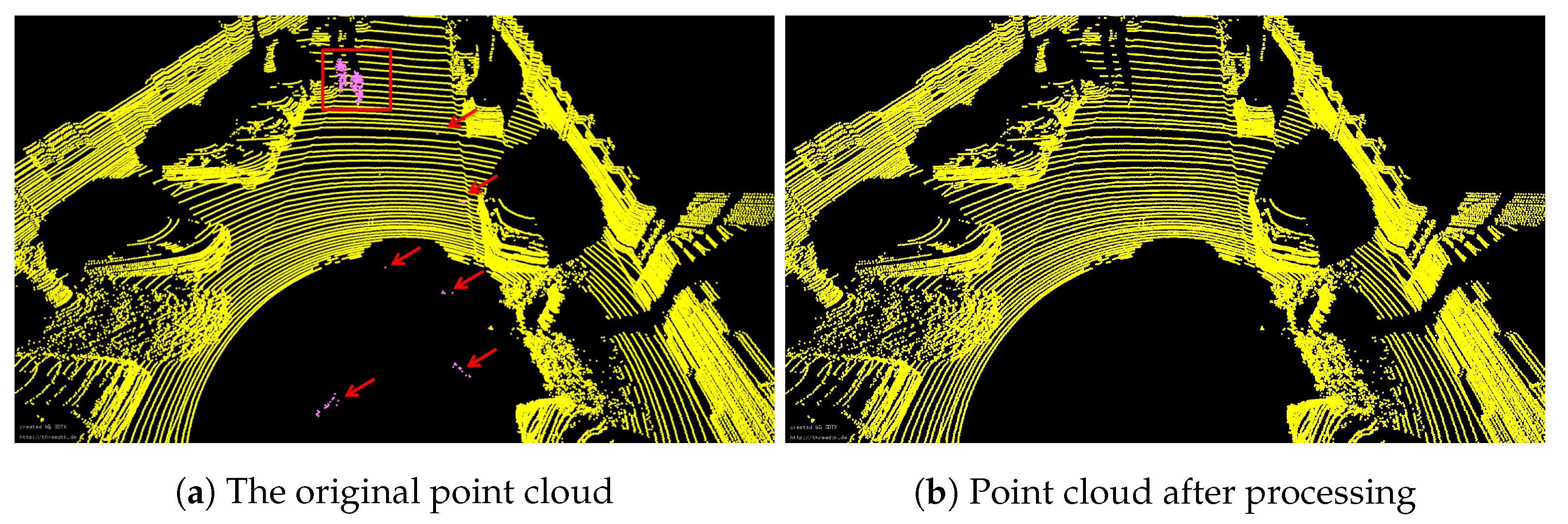
• Point cloud with point-wise semantic labels is used to coarsely remove dynamic objects and outliers. The proposed filtering method largely preserves the static parts of all movable classes while removing dynamic objects and outliers.
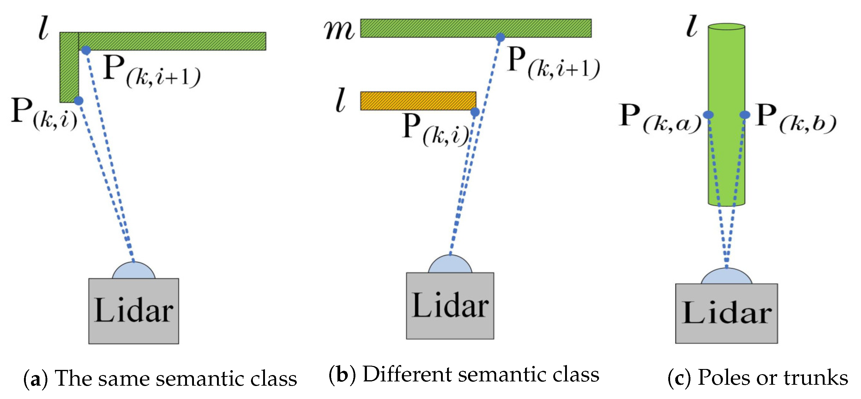
• We use point-wise semantic labels instead of the smoothness of the local surface to extract edge and plane features. Semantic labels are first used to establish candidate feature points. Then, some down-sampling and culling strategies are presented to select feature points from these candidate feature points.
• In the LiDAR odometry and mapping module, we constrain the corresponding points of frame-to-frame or frame-to-map to the same semantic label. Besides, a second dynamic objects filtering strategy is also presented in the mapping module.
• To verify the proposed solution, extensive experiments have been carried out in several scenarios, including the urban, the country and highway, based on the semanticKITTI dataset [33]. Experimental results show that the proposed methods can achieve high-precision positioning and mapping results compared with the state-of-the-art SLAM methods.

The remainder of the paper is structured as follows: In Section 2, the proposed methodology is described in detail. Experimental results are then shown in Section 3, which is followed by a discussion in Section 4. Finally, the paper ends with a conclusion in Section 5.

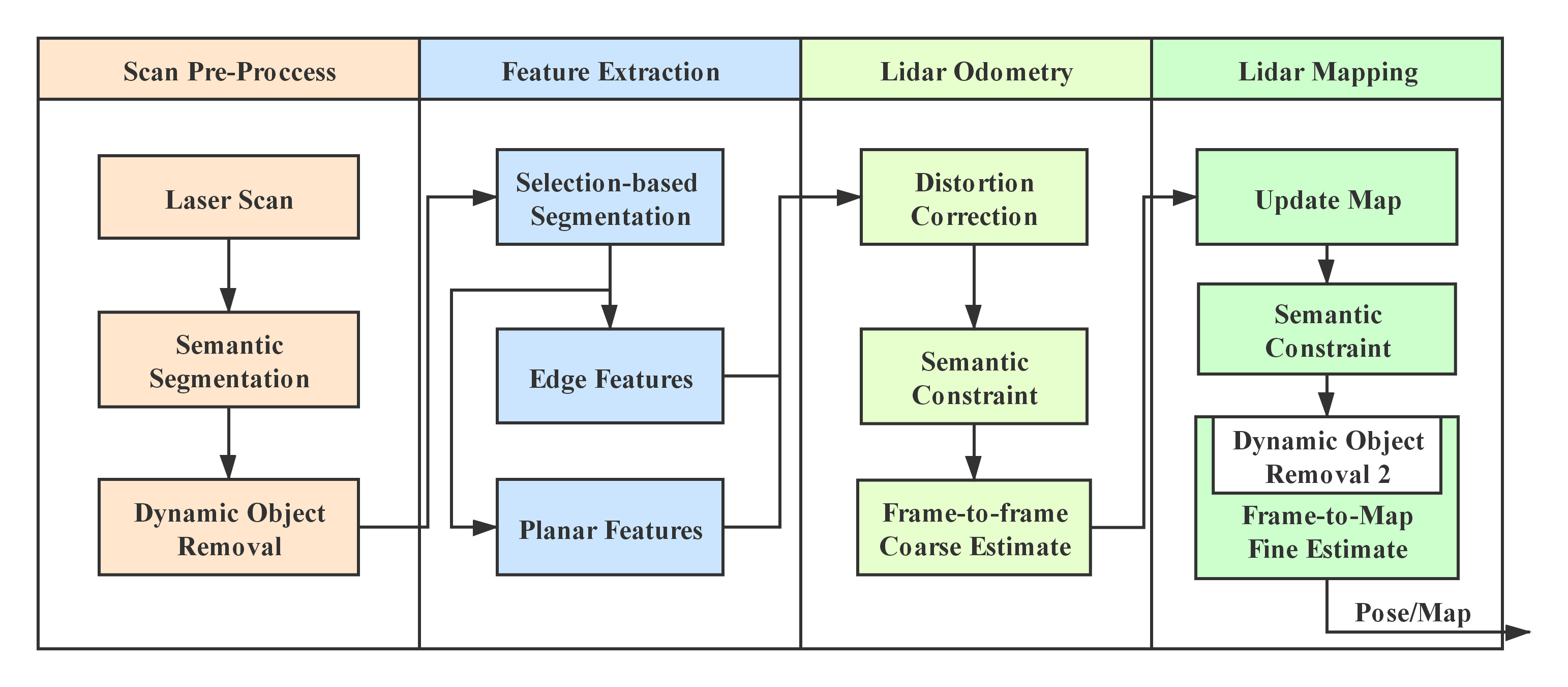
2. Materials and Methods

An overview of our S-ALOAM is shown in Figure 1. The system takes the 3D LiDAR data as inputs and outputs 6 DOF pose estimation and a feature map. The overall system contains four sequential modules. The first, scan pre-processing, utilizes point-wise semantic labels generated by a semantic segmentation network to coarsely remove the dynamic objects and outliers. The remaining segmented point cloud is then input to the feature extraction module, where we extract edge and planar features by semantic labels instead of the smoothness of the local surface. Then, LiDAR odometry estimates the transformation between the consecutive point cloud by combining semantic constraints with geometric features. Meanwhile, this part compensates for any point cloud deformation caused by the LiDAR rotation and vehicle movement. Furthermore, these features are fed into LiDAR mapping, which obtains the accurate pose and feature map estimation by enabling a frame-to-map framework. Moreover, a second dynamic objects filtering strategy is also presented in this step. The details of each module are introduced in the following sections.

2.1. Scan Pre-Processing

The scan pre-processing module consists of point-wise semantic label acquisition and dynamic objects removal. Since we aim to integrate semantic information into the LiDAR SLAM framework, all those semantic segmentation methods that can output point-wise semantic labels can be applied to our system. For example, all semantic segmentation algorithms ranked on the SemanticKITTI benchmark [33] can be integrated into our system. Therefore, in this section, we do not propose a special semantic segmentation method but use a pre-labeled dataset, i.e., SemanticKITTI, to verify the proposed method. The details of the SemanticKITTI dataset will be given in Section 3. By point-wise semantic labels, point cloud can be divided into non-overlapping sub-point clouds with rich semantic attributes, such as pedestrians and cars.

Dynamic objects, such as pedestrians and moving vehicles, will cause wrong associations. A simple solution is to filter out all movable semantic classes, including all vehicles and persons. However, the approach also removes many static objects, such as parked vehicles, which are valuable features for the data association and pose estimation. To this end, we propose a two-step dynamic object removal strategy. In this part, only the first step, the filtering method, is presented, and the second step, the removal strategy, will be shown in the mapping module. Specifically, the coarse filtering method achieves the goal by removing the objects with a larger probability of movement in the environment, which include persons, bicyclists, motorcyclists and railcars. Meanwhile, this step also filters out the points labeled as outliers and unlabeled. Overall, the proposed filtering method largely preserves the static part of all movable classes while removing dynamic objects and noise points.

2.2. Feature Extraction

LOAM and its variants extract edge and planar features by calculating the smoothness of the local surface. To evenly extract features in the environment, they divide a scan line into six equal subregions. Two edge features and four planar features are extracted from each subregion. The method that only relies on the local smoothness cannot guarantee accurate feature extraction. Moreover, one drawback of point-wise extraction is that some subregions without obvious features are forcibly assigned the same number of feature points as other subregions. In this part, we completely improve the feature extraction method of LOAM by considering semantic information.

Different from LOAM, the proposed method works in the point cluster with the same semantic label line-by-line according to the chronological order. Let ${\mathbf{P}}_{(k,i)}^l$ be the ith point of the kth point cloud ${\mathbf{P}}_k$ acquired during the sweep k, ${\mathbf{P}}_{(k,i)}^l\in {\mathbf{P}}_k$. Note that the superscript l indicates the semantic label of point ${\mathbf{P}}_{(k,i)}$. Point ${\mathbf{P}}_{(k,i)}^l$ is selected as an edge point only if one of the following three cases is satisfied.

1. The edge feature can be selected from the same semantic category by:

$$\begin{array}{c}\hfill \parallel {\mathbf{P}}_{(k,i)}^l-{\mathbf{P}}_{(k,i+1)}^l\parallel >th\end{array}$$

(1)

Then, ${\mathbf{P}}_{(k,i)}^l$ is an edge point if (e.g., ${\mathbf{P}}_{(k,i)}^l$ in Figure 2a):

$$\begin{array}{c}\hfill \parallel {\mathbf{P}}_{(k,i)}^l\parallel <\parallel {\mathbf{P}}_{(k,i+1)}^l\parallel \end{array}$$

(2)

Otherwise, if:

$$\begin{array}{c}\hfill \parallel {\mathbf{P}}_{(k,i)}^l\parallel >\parallel {\mathbf{P}}_{(k,i+1)}^l\parallel \end{array}$$

(3)

${\mathbf{P}}_{(k,i+1)}^l$ is selected as an edge point, where ${\mathbf{P}}_{(k,i+1)}^l$ is the nearest measurement point of ${\mathbf{P}}_{(k,i)}^l$ in scanning order, and they have the same semantic label l, which indicates these two points belong to the same category in the real environment. $th$ denotes a threshold, and $\parallel ·\parallel$ represents the Euclidean distance. As shown in Figure 2a, we select the convex points with respect to the center of the LiDAR in the same semantic category as edge points. These points often occur in the real environment (e.g., the intersection of two walls).

2. The edge feature can be selected from the boundary of different semantic categories. Figure 2b intuitively describes the case. ${\mathbf{P}}_{(k,i)}^l$ and ${\mathbf{P}}_{(k,i+1)}^m$ are two consecutive points that belong to two different semantic categories l and m, respectively. Point ${\mathbf{P}}_{(k,i)}^l$ can be treated as the edge point only if:

$$\begin{array}{c}\hfill \parallel {\mathbf{P}}_{(k,i)}^l\parallel <\parallel {\mathbf{P}}_{(k,i+1)}^m\parallel \end{array}$$

(4)

Otherwise, ${\mathbf{P}}_{(k,i+1)}^m$ can be labeled as the edge point. In this case, those boundary points that are closer to the center of the LiDAR between different semantic categories are selected as edge points, such as point ${\mathbf{P}}_{(k,i)}^l$ in Figure 2b.

3. The edge feature extraction in the cylinder-like structures. The edge points are generated when the LiDAR scans the cylinder-like structures (see Figure 2c). To maintain the real-time performance and the invariance of feature points, we extract edge points by downsampling the points of the cylinder-like structure. Specifically, if the number of points on the scan line where the cylinder-like object is located is less than six, the midpoint of these points is selected as the final edge point.

Otherwise, we use these points to fit a circle by least squares. Then, the center of the fitted circle is considered as the edge point on the current scan line. This is based on the recognition that these points of the cylinder-like structure on a scan line can form a circle. Next, we will introduce how to use least squares to fit a circle. As shown in Figure 2c, let $({\mathbf{P}}_{(k,a)}^l,\cdots ,{\mathbf{P}}_{(k,b)}^l)$ be the points of the cylinder-like structure l on the current scan line ($(b-a)>6$). Now, we use these points to fit a circle. The equation of the circle is often defined as follows:

$$\begin{array}{c}\hfill {(x-x_c)}^2+{(y-y_c)}^2=R^2\end{array}$$

(5)

where $(x_c,y_c)$ represent the center of the circle, and R denotes the radius of the circle. The goal of the least-squares-based fitting method is to minimize the following equation:

$$\begin{array}{c}\hfill f=\sum _{i=a}^b{(\sqrt{{(x_i^l-x_c^l)}^2+{(y_i^l-y_c^l)}^2}-R)}^2\end{array}$$

(6)

where $(x_i^l,y_i^l)$, $i=(a,\cdots ,b)$ are coordinates of $P_{(k,i)}^l$ from the cylinder-like structure (labeled semantic classes l) on the current scan line. However, Equation (6) only has the numerical solution that needs to be calculated iteratively. To obtain the analytical solution that also meets the real-time requirements, we simplify it slightly as follows:

$$\begin{array}{c}\hfill \widehat{f}=\sum _{i=a}^b{({(x_i^l-x_c^l)}^2+{(y_i^l-y_c^l)}^2-R^2)}^2\end{array}$$

(7)

Let $g(x,y)={(x-x_c^l)}^2+{(y-y_c^l)}^2-R^2$. Equation (7) can be expressed as:   

$$\begin{array}{c}\hfill \widehat{f}=\sum _{i=a}^{b}g{(x_i^l,y_i^l)}^2\end{array}$$

(8)

By now, Equation (8) can be solved by partial derivatives. Specific calculation details are not given in this paper. In summary, edge features are extracted by the above strategies. In contrast, it is easier to extract planar features. In our system, all points of semantic classes with plane attributes, such as road, sidewalk, traffic-sign and cars, are considered as planar features. Of course, those edge points that satisfy the above conditions are excluded.

After feature extraction, The sets of edge features ${\mathbb{E}}_k$ and plane features ${\mathbb{H}}_k$ of the current time k are obtained. Here, we also obtain the edge features ${\mathcal{E}}_k$ and plane features ${\mathcal{H}}_k$ by downsampling ${\mathbb{E}}_k$ and ${\mathbb{H}}_k$, respectively. Thus, we have ${\mathcal{E}}_k\subset {\mathbb{E}}_k$ and ${\mathcal{H}}_k\subset {\mathbb{H}}_k$. Specifically, the edge points ${\mathcal{E}}_k$ are selected by uniformly-sampling ${\mathbb{E}}_k$, while plane features ${\mathcal{H}}_k$ are selected by taking the center point of the point cluster with plane attributes on each scan line.

The proposed method follows a similar framework in LOAM, i.e., the line-by-line extraction and piecewise extraction in scanning order. However, we completely consider the semantic information instead of the local smoothness for feature selection criteria. In addition, LOAM forcibly divides each scan line into six uniform segments, which may break the coherence of feature extraction. By contrast, our segmentation extraction is completely based on semantic categories, which is more consistent with the distribution of feature points in the real environment.

2.3. LiDAR Odometry

This module includes deformation correction and LiDAR odometry. To clearly describe this section, we start with the deformation correction module, which is followed by the LiDAR odometry module.

2.3.1. Deformation Correction

Mobile vehicles equipped with LiDAR acquire the point cloud by rotating the laser beam while moving forward. Obviously, vehicle movements during the point cloud acquisition will deform the point cloud. To address this, some methods need to be used to compensate for the deformation. In this part, we adopt the same method as LOAM, namely linear interpolation, which models the motion within the point cloud as the constant angular and linear velocity motion.

Denote $t_k$ the end time of the current point cloud ${\mathbf{P}}_k$. Furthermore, $t_{k-1}$ is the starting time of the current point cloud ${\mathbf{P}}_k$ or the end time of the previous point cloud ${\mathbf{P}}_{k-1}$. Thus, ${\mathbf{T}}_{k-1}^k$ represents the relative motion transform of the vehicle between $[t_{k-1},t_k]$. Given a laser point ${\mathbf{P}}_{(k,i)}$, ${\mathbf{P}}_{(k,i)}\in {\mathbf{P}}_k$, let $t_{(k,i)}\in [t_{k-1},t_k]$ be its timestamp. Consequently, the relative pose transform ${\mathbf{T}}_{(k,i)}$ between $[t_{k-1},t_{(k,i)}]$ can be computed as:

$$\begin{array}{c}\hfill {\mathbf{T}}_{(k,i)}=\frac{t_{(k,i)}-t_{k-1}}{t_{scan}}{\mathbf{T}}_{k-1}^k\end{array}$$

(9)

where $t_{scan}$ represents the scanning period of a point cloud. Thus, non-deformable point clouds ${\overline{\mathbb{E}}}_k$ and ${\overline{\mathbb{H}}}_k$ are obtained by projecting ${\mathbb{E}}_k$ and ${\mathbb{H}}_k$ to the end of the sweep k, i.e., $t_k$, by:

$$\begin{array}{c}\hfill {\mathbb{P}}_{(k,i)}^s={\mathbf{R}}_{(k,i)}{\mathbb{P}}_{(k,i)}+{\mathbf{D}}_{(k,i)}\end{array}$$

(10)

$$\begin{array}{c}\hfill {\overline{\mathbb{P}}}_{(k,i)}={\mathbf{R}}_{k-1}^k({\mathbb{P}}_{(k,i)}^s-{\mathbf{D}}_{k-1}^k)\end{array}$$

(11)

where ${\mathbb{P}}_{(k,i)}$ is a feature point of ${\mathbb{E}}_k$ or ${\mathbb{H}}_k$. Furthermore, ${\mathbf{R}}_{(k,i)}$ and ${\mathbf{D}}_{(k,i)}$ are rotation matrix and translation vector of ${\mathbf{T}}_{(k,i)}$, respectively. ${\mathbf{R}}_{k-1}^k$ and ${\mathbf{D}}_{k-1}^k$ denote the rotation matrix and translation vector of ${\mathbf{T}}_{k-1}^k$, which represents the relative motion transform between $[t_{k-1},t_k]$. ${\overline{\mathbb{P}}}_{(k,i)}$ is the corresponding non-deformable feature in feature point set ${\overline{\mathbb{E}}}_{k-1}$ and ${\overline{\mathbb{H}}}_{k-1}$. We first project ${\mathbb{P}}_{(k,i)}$ to the initial moment of the current point cloud $t_{k-1}$. Therefore, ${\mathbb{P}}_{(k,i)}^s$ is obtained. Then, ${\mathbb{P}}_{(k,i)}^s$ is transformed to the end of the sweep k by ${\mathbf{T}}_{k-1}^k$.

2.3.2. LiDAR Odometry

The basic algorithm of this part is consistent with LOAM, but semantic constraints are introduced when searching for corresponding points. Therefore, in order to clearly describe how semantic information assists the corresponding point search, we re-discuss this part. The purpose of the LiDAR odometry module is to estimate the LiDAR transformation between two consecutive point clouds by minimizing point-to-edge and point-to-plane distance functions. To find corresponding points between current point cloud ${\mathbf{P}}_k$ and the previous point cloud ${\mathbf{P}}_{k-1}$, ${\mathcal{E}}_k$ and ${\mathcal{H}}_k$ are projected to the beginning of the sweep k, i.e., ${\tilde{\mathcal{E}}}_k$ and $\widetilde{{\mathcal{H}}_k}$. The mathematical operation is given as follows:

$$\begin{array}{c}\hfill {\tilde{\mathbf{P}}}_{(k,i)}={\mathbf{R}}_{(k,i)}{\mathbf{P}}_{(k,i)}+{\mathbf{D}}_{(k,i)}\end{array}$$

(12)

where ${\mathbf{R}}_{(k,i)}$ and ${\mathbf{D}}_{(k,i)}$ are rotation matrix and translation vector of ${\mathbf{T}}_{(k,i)}$, respectively. ${\mathbf{P}}_{(k,i)}$ is a feature point of ${\mathcal{E}}_k$ or ${\mathcal{H}}_k$. Furthermore, ${\tilde{\mathbf{P}}}_{(k,i)}$ is the corresponding feature in feature point set ${\tilde{\mathcal{E}}}_k$ or $\widetilde{{\mathcal{H}}_k}$.

For each feature in ${\tilde{\mathcal{E}}}_k$ and $\widetilde{{\mathcal{H}}_k}$, we start to search for the closest neighbor point in ${\overline{\mathbb{E}}}_{k-1}$ and ${\overline{\mathbb{H}}}_{k-1}$. The point-to-edge scan matching is performed by minimizing the distance of each edge line in ${\overline{\mathbb{E}}}_{k-1}$ to the edge point in ${\tilde{\mathcal{E}}}_k$. Furthermore, the edge line is represented by two edge points on adjacent scan lines. The point to edge line distance is defined as:

$$\begin{array}{c}\hfill d_{\mathcal{E}}=\frac{|({\tilde{\mathcal{E}}}_{(k,i)}^l-{\overline{\mathbb{E}}}_{(k-1,j)}^l)\times ({\tilde{\mathcal{E}}}_{(k,i)}^l-{\overline{\mathbb{E}}}_{(k-1,q)}^l)|}{\left|\right({\overline{\mathbb{E}}}_{(k-1,j)}^l-{\overline{\mathbb{E}}}_{(k-1,q)}^l\left)\right|}\end{array}$$

(13)

where ${\overline{\mathbb{E}}}_{(k-1,j)}^l$ and ${\overline{\mathbb{E}}}_{(k-1,q)}^l$ are points of ${\overline{\mathbb{E}}}_{k-1}$ from the previous point cloud. Furthermore, ${\tilde{\mathcal{E}}}_{(k,i)}^l$ is an edge feature in ${\tilde{\mathcal{E}}}_k$ from the current point cloud. The superscript l indicates the semantic label of the point.

Furthermore, the point-to-plane scan matching is performed by minimizing the distance of each planar patch in ${\overline{\mathbb{H}}}_{k-1}$ to the planar point in $\widetilde{{\mathcal{H}}_k}$. Furthermore, the planar patch is formed by three planar features on adjacent scan lines. The point-to-plane distance is then computed as:

$$\begin{array}{c}\hfill d_{\mathcal{H}}=\frac{\left|\begin{array}{c}({\tilde{\mathcal{H}}}_{(k,i)}^m-{\overline{\mathbb{H}}}_{(k-1,j)}^m)(({\overline{\mathbb{H}}}_{(k-1,j)}^m-{\overline{\mathbb{H}}}_{(k-1,q)}^m)\times ({\overline{\mathbb{H}}}_{(k-1,j)}^m-{\overline{\mathbb{H}}}_{(k-1,r)}^m))\end{array}\right|}{|({\overline{\mathbb{H}}}_{(k-1,j)}^m-{\overline{\mathbb{H}}}_{(k-1,q)}^m)\times ({\overline{\mathbb{H}}}_{(k-1,j)}^m-{\overline{\mathbb{H}}}_{(k-1,r)}^m)|}\end{array}$$

(14)

where points ${\overline{\mathbb{H}}}_{(k-1,j)}^m$, ${\overline{\mathbb{H}}}_{(k-1,q)}^m$ and ${\overline{\mathbb{H}}}_{(k-1,r)}^m$ form the corresponding planar patch. The superscript m indicates the semantic label of the point.

Combining Equations (9)–(14), a nonlinear function based on the point to the edge line distance is calculated as follows:

$$\begin{array}{c}\hfill f_{\mathcal{E}}({\mathcal{E}}_{(k,i)},{\mathbf{T}}_{k-1}^k)=d_{\mathcal{E}}\end{array}$$

(15)

Furthermore, a nonlinear function based on the point to planar distance is calculated as follows:

$$\begin{array}{c}\hfill f_{\mathcal{H}}({\mathcal{H}}_{(k,i)},{\mathbf{T}}_{k-1}^k)=d_{\mathcal{H}}\end{array}$$

(16)

Substitute each feature point of ${\mathcal{E}}_k$ and ${\mathcal{H}}_k$ into Equations (15) and (16), and the final nonlinear function to be optimized is defined as:   

$$\begin{array}{c}\hfill \mathbf{f}\left({\mathbf{T}}_{k-1}^k\right)=\left(\begin{array}{c}{\mathbf{d}}_{\mathcal{E}}\\ {\mathbf{d}}_{\mathcal{H}}\end{array}\right)=\mathbf{d}\end{array}$$

(17)

where ${\mathbf{d}}_{\mathcal{E}}$ and ${\mathbf{d}}_{\mathcal{H}}$ consist of the corresponding distance function of each feature point in ${\mathcal{E}}_k$ and ${\mathcal{H}}_k$, respectively. The goal of LiDAR odometry is to calculate ${\mathbf{T}}_{k-1}^k$ by iteratively minimizing $\mathbf{d}$ towards zero.

$$\begin{array}{c}\hfill {\mathbf{T}}_{k-1}^k\leftarrow {\mathbf{T}}_{k-1}^k-{({\mathbf{J}}^T\mathbf{J}+\lambda diag\left({\mathbf{J}}^T\mathbf{J}\right))}^{-1}{\mathbf{J}}^T\mathbf{d}\end{array}$$

(18)

where $\mathbf{J}=\partial \mathbf{f}/\partial {\mathbf{T}}_{k-1}^k$. Furthermore, $\lambda$ is a factor of the nonlinear optimization algorithm such as the Levenberg–Marquardt method.

Assume the LiDAR coordinate system $\left\{L\right\}$ coincides with the world coordinate system $\left\{W\right\}$ at the initial time $t_0$. ${\mathbf{T}}_k^W$ can be calculated by accumulating the relative motion ${\mathbf{T}}_{k-1}^k$ of all previous adjacent locations up to the current location k.

Compared to LOAM, we introduce semantic constraints in Equations (13) and (14), namely, the correspondences are only found in feature points with the same semantic label from ${\overline{\mathbb{E}}}_{k-1}$ and ${\overline{\mathbb{H}}}_{k-1}$. For example, in Equation (13), ${\tilde{\mathcal{E}}}_{(k,i)}^l$ has the same semantic label l as points ${\overline{\mathbb{E}}}_{(k-1,j)}^l$ and ${\overline{\mathbb{E}}}_{(k-1,q)}^l$. Searching for the correspondences between the same semantic classes are more likely to find the correct correspondences. Furthermore, this can greatly improve the efficiency and accuracy of scan matching.

2.4. Lidar Mapping

After the LiDAR odometry algorithm, non-deformable point clouds ${\overline{\mathbb{E}}}_k$ and ${\overline{\mathbb{H}}}_k$ are obtained, and simultaneously LiDAR odometry also output ${\mathbf{T}}_k^W$, which indicates the pose of the current point cloud ${\mathbf{P}}_k$ in the world coordinate system $\left\{W\right\}$. Let $Q_{k-1}^{\mathcal{E}}$ and $Q_{k-1}^{\mathcal{H}}$ be the edge features and planar features on the map, respectively, accumulated until time $k-1$. The LiDAR mapping module matches features in $\{{\overline{\mathbb{E}}}_k,{\overline{\mathbb{H}}}_k\}$ to the global map to optimize the pose estimation.

The pseudocode of the LiDAR mapping is presented in Algorithm 1. The pose ${\mathbf{T}}_k^W$ generated by the LiDAR odometry module is set as the initial guess (line 1). Parameter $ite{r}_{max}$ indicates the maximum number of iterations (line 2). To find corresponding points between the current point cloud ${\mathbf{P}}_k$ and the global map accumulated until time $k-1$, ${\overline{\mathbb{E}}}_k$ and ${\overline{\mathbb{H}}}_k$ are projected to the world coordinate system $\left\{W\right\}$ (line 4 and line 12). The mathematical operation is given as follows:

$$\begin{array}{c}\hfill {\mathbf{P}}_{(k,i)}^w={\mathbf{R}}_k^w{\overline{\mathbf{P}}}_{(k,i)}+{\mathbf{D}}_k^w\end{array}$$

(19)

where ${\mathbf{R}}_k^w$ and $D_k^w$ are rotation matrix and translation vector of ${\mathbf{T}}_k^W$, respectively. ${\overline{\mathbf{P}}}_{(k,i)}$ is a feature point of ${\overline{\mathbb{E}}}_k$ or ${\overline{\mathbb{H}}}_k$. Lines 6–7 and lines 14–15 are implemented by computing the covariance matrix, eigenvalues and eigenvectors. Readers can refer to [29] for the detailed description. After this process, we can compute the point-to-line distance (lines 7–8) and the point-to-planar distance (lines 15–16) by Equation (13) and Equation (14), respectively. Compared to the LiDAR mapping module in LOAM, we introduce semantic constraints, namely, these five nearest points found in $Q_{k-1}^{\mathcal{E}}$ or $Q_{k-1}^{\mathcal{H}}$ have the same semantic label as ${\overline{\mathbf{P}}}_{(k,i)}$ in ${\overline{\mathbb{E}}}_k$ or ${\overline{\mathbb{H}}}_k$. Then, ${\tilde{\mathbf{T}}}_k^W$ is updated (lines 22–27) based on Equation (18) as in Section 2.3.2.

As mentioned earlier, a second step dynamic objects filtering strategy is also presented in this section. This method was first proposed in [49]. Specifically, after all residual blocks are added, we first calculate ${\tilde{\mathbf{T}}}_k^W$ by one iteration (line 19). ${\tilde{\mathbf{T}}}_k^W$ is then used to recompute all residuals in Equation (17) (line 20), and feature points with the first 10% largest residuals are removed (line 21). After this step, the full iterative update is finally performed. The above dynamic objects filtering method is proposed based on the assumption that the dynamic points can lead to large distance errors in point cloud matching.

Algorithm 1 LiDAR Mapping.

Input:  ${\overline{\mathbb{E}}}_k$ and ${\overline{\mathbb{H}}}_k$ from the ${\mathbf{P}}_k$, the point cloud map $Q_{k-1}^{\mathcal{E}}$ and $Q_{k-1}^{\mathcal{H}}$, accumulated until the last point cloud. ${\mathbf{T}}_k^W$ from the LiDAR odometry. Output:  The optimized pose ${\tilde{\mathbf{T}}}_k^W$. 1: Initialization: ${\tilde{\mathbf{T}}}_k^W\leftarrow {\mathbf{T}}_k^W$ 2: fori = 0; i $<ite{r}_{max}$; $i++$ do 3:     for ${\overline{\mathbf{P}}}_{(k,i)}$∈${\overline{\mathbb{E}}}_k$ do 4:         Compute ${\mathbf{P}}_{(k,i)}^w$ via Equation (19) 5:         Find 5 nearest points of ${\mathbf{P}}_{(k,i)}^w$ in $Q_{k-1}^{\mathcal{E}}$ 6:         if these five nearest points are indeed in a line then 7:            Compute point to line distance which is similar to Equation (13) 8:            and add the residual $d_{\mathcal{E}}$ which is similar to (17); 9:         end if 10:     end for 11:     for ${\overline{\mathbf{P}}}_{(k,i)}$∈${\overline{\mathbb{H}}}_k$ do 12:         Compute ${\mathbf{P}}_{(k,i)}^w$ via Equation (19) 13:         Find 5 nearest points of ${\mathbf{P}}_{(k,i)}^w$ in $Q_{k-1}^{\mathcal{H}}$ 14:         if these five nearest points are indeed a plane then 15:            Compute point to planar distance which is similar to Equation (14) 16:            and add the residual $d_{\mathcal{H}}$ which is similar to (17); 17:         end if 18:     end for 19:     Perform pose optimization with 1 iteration based on Equation (18). 20:     recompute ${\mathbf{d}}_{\mathcal{E}}$ and ${\mathbf{d}}_{\mathcal{H}}$ in Equation (17), 21:     then remove 10% of the biggest residuals 22:     for a maximal number of iterations do 23:         Perform pose optimization based on Equation (18) 24:         if the nonlinear optimization converges then 25:            break; 26:         end if 27:     end for 28: end for

3. Results

3.1. Experimental Platform and Evaluation Method

In this paper, we do not propose a semantic segmentation algorithm but evaluate the proposed algorithm on SemanticKITTI, which is a point-wise annotated point cloud dataset based on the KITTI Vision Benchmark. Since semantic segmentation is not the focus of this paper, we aim to explore the application of the prior semantic information in the LiDAR SLAM framework. Hence, the proposed method is not limited to a specific semantic segmentation method. Therefore, all those semantic segmentation methods that can output point-wise semantic labels can be applied to our system.

SemanticKITTI provides accurate point-wise annotation with 34 semantic classes for 22 sequences of LiDAR data on the KITTI Vision Benchmark [50]. Furthermore, point clouds from sequences 00 to 10 are training sets with the available labels, and the remaining sequences are used as the test set. Figure 3 is a visual inspection from a single scan with semantic annotations in SemanticKITTI. As shown in Figure 3, objects with the same semantic attribute are displayed in the same color, e.g., pink represents the ground, and yellow indicate the vehicle.

The LiDAR data in the KITTI Vision Benchmark is recorded with a Velodyne HDL-64E laser scanner at a rate of 10 Hz. It provides 22 sequences of point cloud data, which contain 11 training data sets with ground truth and 11 test data sets without ground truth. These sequences include multiple environments ranging from the busy city to highway traffic. The ground truth is provided by a high accuracy GPS/INS navigation system. We test our approach on the desktop computer with an i7-7700 3.60 GHz CPU. All algorithms are implemented in C++ and executed on Ubuntu 16.04.

Table 1. The KITTI sequences used in our experiment.

Sequences	Number of Scans	Distance (m)	Environment
00	4541	3714	Urban
01	1101	2453	Highway
02	4661	5067	Urban + Country
04	271	394	Country
07	1101	694	Urban
08	4071	3223	Urban + Country

shows the KITTI sequences used in our experiment. To verify the robustness of the algorithm, we selected 6 typical sequences of 11 sequences. The reason of selecting these six sequences is they cover all the situations that our algorithm might encounter in reality. First, in terms of scenarios, these sequences cover a variety of environments, including urban (00,07), highway (01), country (04) and their fusion (02, 08). Then, as for the trajectory length, the longest path reaches 5067 m (02), while the shortest mileage is only 394 m (04). Moreover, the vehicle speed of the vehicle in sequence 01 reaches 85 km/h (01). Moreover, some of these sequences have loops (00,02,07,08), while others have no loops (01,04). In short, the six sequences selected above can fully verify the performance of the proposed algorithm.

The proposed algorithm is evaluated by computing the absolute errors in [51] and relative errors in [50], respectively. The absolute metric includes the absolute root-mean-square error (RMSE) in respect to the translation and rotation over all point clouds, respectively. To compare our approach against the state-of-the-art SLAM methods, the relative errors are computed by averaging relative translation and rotation errors using different trajectory distances. Next, we will evaluate the proposed algorithm from three aspects, i.e., dynamic object removal, feature extraction and pose estimation.

3.2. Dynamic Object Removal

Moving objects in the point cloud will cause large errors when matching. Here, we propose a simple but effective method to coarsely remove dynamic objects and outliers. According to semantic labels provided by SemanticKITTI, we remove points labeled as person, bicyclist, motorcyclist, railcars, outliers and unlabeled. Figure 4a shows a point cloud where dynamic objects and outliers are displayed in pink (marked by red rectangle and arrows). After our method, these points are completely culled (see Figure 4b). Compared with the naive method, which filters out all movable semantic classes, including all vehicles and persons, our method effectively removes objects with a larger probability of movement in the environment, such as person, bicyclist, motorcyclist and railcars, while keeping features from static objects, e.g., parked vehicles. These static objects are valuable features for the data association and pose estimation. Meanwhile, this step also removes the points labeled as outliers (red arrow in Figure 4a). However, moving vehicles are not considered in this step. They will be solved in the LiDAR mapping module.

3.3. Feature Extraction Results

To evaluate the accuracy of the semantic label-based feature extraction algorithm, a representative urban environment is selected that is an intersection with parked cars, street lights, trees and buildings. The result is shown in Figure 5. Edge and planar features are colored red and blue, respectively. Solid yellow rectangles mark the feature point extraction on parked cars. As shown in Figure 5a, only a few edge features are extracted from the parked cars in A-LOAM. This is because the space between cars is too close, and the smoothness-based feature extraction method cannot extract effective edge features from the objects next to each other. In contrast, our extraction algorithm shows excellent results on parked cars (see solid yellow rectangles in Figure 5b). This corresponds to the extraction cases in Figure 2a,b.

Solid yellow ellipses mark edge features on cylinder objects. Cylinder objects, e.g., poles and trunks, contain remarkable edge points. However, these features were mistakenly extracted as planar features in A-LOAM (see red points in solid yellow ellipses of Figure 5a). As solid yellow ellipses in Figure 5b show, our semantic label-based extraction algorithm can achieve accurate edge features on poles and trunks. This corresponds to the extraction method in Figure 2c. Dotted yellow ellipses in Figure 5 mark edges feature at the junction of the sidewalk and the road. Figure 5b shows our method completely extracts these edge features, which corresponds to the extraction method in Figure 2b.

In addition to the above, A-LOAM also mistakenly extracts some points as edge points. For example, red points marked by dotted yellow rectangles in Figure 5a. These points are from the junction of the starting and ending positions of a LiDAR scan circle. Due to the influence of motion deformation, there is a large distance between points at the starting position and the ending position, and the extraction method that uses the distance to calculate the smoothness will mistake them as edge points. As a result, these points are always extracted as edge points when the LiDAR moves forward. Further, some outliers are extracted as edge features in A-LOAM, as shown in Figure 5a (marked by yellow arrows). By contrast, our semantic label-based method completely removes these false edge extractions. As for planar features, our method and A-LOAM show similar performances in Figure 5. However, we only extract planar features from objects with plane attributes, such as roads, sidewalks, buildings, traffic-signs and cars. This greatly increases the accuracy of planar feature extraction.

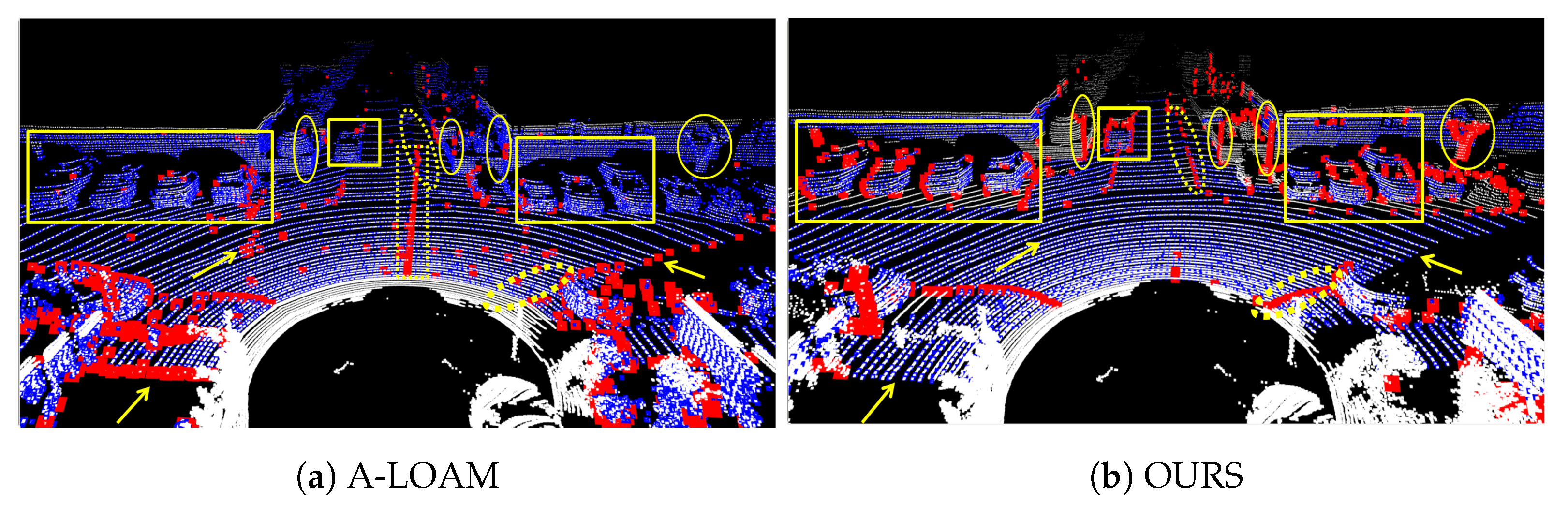
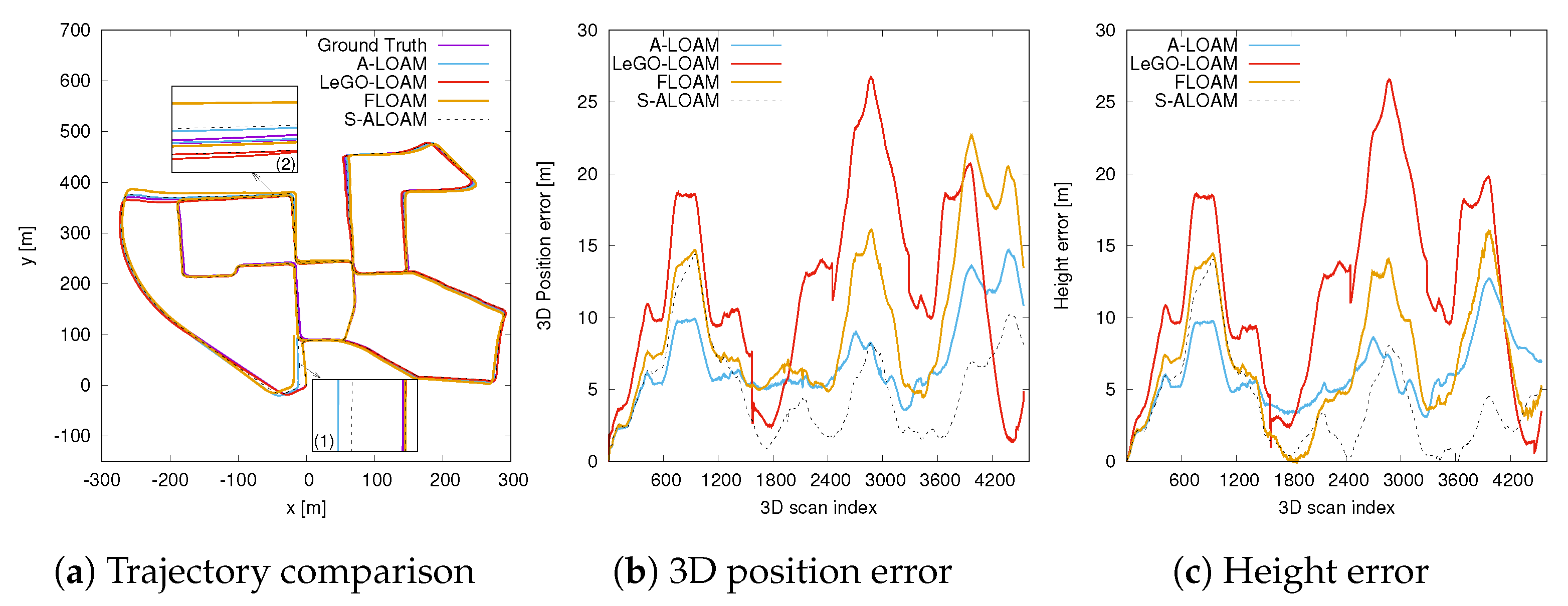
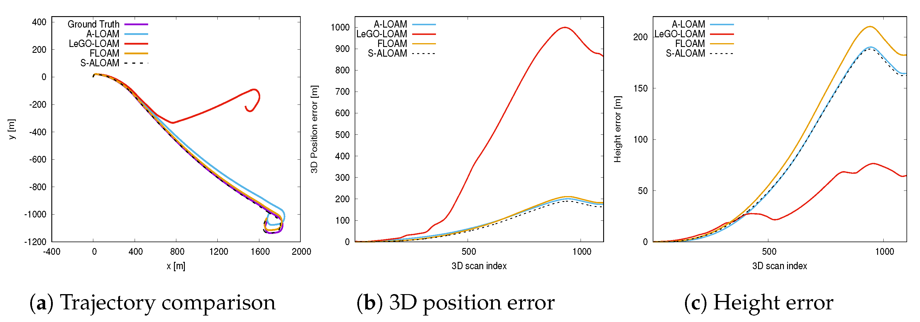
3.4. Pose Estimation Comparison

In this part, we compare the accuracy and robustness of the proposed method S-ALOAM with the current state-of-the-art algorithms, namely A-LOAM, LeGO-LOAM and FLOAM [52], in various challenging outdoor environments. The framework and basic principles of FLOAM are similar to A-LOAM, but it optimizes the A-LOAM algorithm, which improves the computational efficiency by three times. Next, we will use the six-sequence dataset with semantic labels described in Table 1 to evaluate the proposed algorithm. This experiment first conducted a detailed analysis on the trajectory error comparison graphs of three sequences. These sequences cover urban, highways and complex mixed scenes. Then, the quantitatively absolute and relative errors of all six sequences are given.

Figure 6 shows the trajectory comparison graph of the sequence 00, which is collected in urban. As Figure 6a shows, the proposed approach, S-ALOAM, generates more consistent trajectories than other methods. This shows semantic labels-based feature extraction does improve the performance. However, compared with LeGO-LOAM, the other three methods suffer accumulation errors in loop closures. As Figure 6a(1),a(2) show, there are large gaps when the robot revisits the same place. By contrast, LeGO-LOAM performs better in loop closures. This is because loop closure constraints of LeGO-LOAM correct the accumulated drift. Meanwhile, Figure 6b,c show similar error curves, which demonstrates the position error is mainly caused by height errors in LOAM and its variants.

The position errors of all algorithms reach the first peak at scan 943 (see Figure 6b,c). Figure 7a is the real image corresponding to scan 943, we can see that the car is turning left and going downslope. This shows LOAM and its variants cannot correctly estimate height in environments with turning and slope. By contrast, A-LOAM has a smaller error here, while FLOAM and S-ALOAM show similar accuracy. Furthermore, LeGO-LOAM performs worst here. The reason is LeGO-LOAM cannot accurately extract the ground in such an environment, which leads to large height errors. After scan 943, S-ALOAM achieves, for the most part, a lower translational and height error.

Table 2. The absolute errors of the proposed method (S-ALOAM) compared with A-LOAM, LeGO-LOAM and FLOAM, where $t_{abs}$ represents the root-mean-square error (RMSE) of translations, while $r_{abs}$ represents rotation error. n.a. in this table indicates the rotation part of LeGO-LOAM is not available. Bold indicates the best result.

Sequence	A-LOAM		LeGO-LOAM		FLOAM		S-ALOAM
	${\mathit{t}}_{\mathit{abs}}$ (m)	${\mathit{r}}_{\mathit{abs}}$ (deg)	${\mathit{t}}_{\mathit{abs}}$ (m)	${\mathit{r}}_{\mathit{abs}}$ (deg)	${\mathit{t}}_{\mathit{abs}}$ (m)	${\mathit{r}}_{\mathit{abs}}$ (deg)	${\mathit{t}}_{\mathit{abs}}$ (m)	${\mathit{r}}_{\mathit{abs}}$ (deg)
00	7.6741	$\mathbf{1}.\mathbf{8436}$	13.8302	n.a.	$8.1101$	2.9859	$\mathbf{6}.\mathbf{2357}$	1.9447
01	114.8519	$\mathbf{7}.\mathbf{0807}$	586.9212	n.a.	$118.6060$	7.6786	$\mathbf{106}.\mathbf{2324}$	7.0901
02	157.2780	32.4780	88.3942	n.a.	$\mathbf{38}.\mathbf{1684}$	$\mathbf{5}.\mathbf{5698}$	$\mathbf{46}.\mathbf{1600}$	$\mathbf{6}.\mathbf{4704}$
04	$\mathbf{2}.\mathbf{1462}$	$\mathbf{0}.\mathbf{8338}$	4.9123	n.a.	2.8831	1.1383	2.9541	1.1444
07	1.0154	$\mathbf{0}.\mathbf{7329}$	2.0474	n.a.	$1.3097$	0.8264	$\mathbf{0}.\mathbf{8988}$	0.9361
08	$\mathbf{17}.\mathbf{1512}$	$\mathbf{2}.\mathbf{4255}$	21.0646	n.a.	20.9252	3.7745	17.9965	3.6825

shows the absolute root-mean-square translation and rotation errors. As shown in Table 2 (00), S-ALOAM is superior to other methods in the translation estimation. Furthermore, it achieves a similar performance to A-LOAM in the rotation estimation.

Figure 8 compares the trajectory error from a highway scene. As Figure 8a shows, S-ALOAM performs better compared to A-LOAM, LeGO-LOAM and FLOAM. The unsatisfactory performance of A-LOAM, LeGO-LOAM and FLOAM is caused by the low geometric structure and many fast-moving dynamic objects in highway scene. Figure 7b presents a photo corresponding to sequence 01. We can see that the environment contains many vehicles moving at a high speed and has only very few geometric structures. Most of the point cloud obtained in such a challenging environment is ground points, and only a few are from traffic signs and sparse trees. In this challenging environment, the purely geometric approach cannot obtain the correct data association, which eventually leads to a large trajectory error.

By comparing Figure 8a with Figure 8c, we can see the errors of S-ALOAM are mainly from height errors, which shows S-ALOAM achieves more accurate pose estimates in $[x,y,{\theta }_{yaw}]$. This is because our semantic label-based feature extraction method can obtain accurate edge features that contribute three degrees of freedom for the pose, i.e., $[x,y,{\theta }_{yaw}]$. Furthermore, there are many factors that cause height errors. First, few distinct structures and the incomplete removal of dynamic vehicles lead to wrong data association. Then, the height is mainly estimated by matching planar features. We extract plane extraction by simply downsampling points with plane attributes. Those uneven planes, for example, roads, that include many slopes will limit the correct estimation of height information. However, as Table 2 (01) shows, S-ALOAM achieves more accurate estimates of the height and also another translation, which is attributed to the semantic constraints and the two-step dynamic object removal strategy. Note that Figure 8c shows that LeGO-LOAM seems to achieve the most accurate height estimation. However, we can find from Figure 8a that LeGO-LOAM fails in the challenging environment.

We also evaluate the proposed method in a mixed scene, including an urban area and the country. Figure 9a shows S-ALOAM is slightly worse than A-LOAM in terms of 2D trajectory, which is mainly due to the fact that the three degrees of freedom $[x,y,{\theta }_{yaw}]$ are mainly estimated by the edge features. We can see from Figure 10b that the environment contains plenty of vegetation, which is extracted as edge features in S-ALOAM. This may lead to the wrong data association when calculating point-to-edge distance. However, we have to keep this vegetation for edge points extraction in the country and highway where few geometric structures exist (see Figure 10b). Figure 9c shows that S-ALOAM achieves more accurate height estimates. Overall, our approach is only slightly inferior to A-LOAM and outperforms LeGO-LOAM and FLOAM (see Table 2 (08)).

The absolute errors of the remaining sequences (02, 04, 07) are also given in Table 2.

Table 3. The relative errors per 100 m, where $t_{rel}$ represents root-mean-square error (RMSE) of translations, while $r_{rel}$ represents rotation error. Because LeGO-LOAM suffers large errors, the corresponding errors are not given here. Bold indicates the best result. Note that rotation error has no unit.

Sequence	A-LOAM		FLOAM		S-ALOAM
	${\mathit{t}}_{\mathit{rel}}$ (m)	${\mathit{r}}_{\mathit{rel}}$	${\mathit{t}}_{\mathit{rel}}$ (m)	${\mathit{r}}_{\mathit{rel}}$	${\mathit{t}}_{\mathit{rel}}$ (m)	${\mathit{r}}_{\mathit{rel}}$
00	1.1639	0.0205	1.0536	0.0206	$\mathbf{1}.\mathbf{0373}$	$\mathbf{0}.\mathbf{0193}$
01	1.0312	$\mathbf{0}.\mathbf{0127}$	1.0533	0.0140	$\mathbf{0}.\mathbf{9621}$	0.0142
02	55.7849	32.4780	1.0397	$\mathbf{0}.\mathbf{0157}$	$\mathbf{0}.\mathbf{9593}$	0.0194
04	$\mathbf{0}.\mathbf{5825}$	$\mathbf{0}.\mathbf{0096}$	0.5970	0.0123	0.6677	0.0143
07	0.5590	$0.0129$	0.5478	$\mathbf{0}.\mathbf{0110}$	$\mathbf{0}.\mathbf{5080}$	0.0154
08	$1.3467$	$\mathbf{0}.\mathbf{0142}$	$\mathbf{1}.\mathbf{2743}$	0.0143	1.3818	0.0154

shows the relative errors of all sequences that are evaluated using evo [53]. The relative error evaluates the local accuracy (drift) of the trajectory. We can see from Table 2 and Table 3 that in most sequence, S-ALOAM is superior to A-LOAM and FLOAM in the translation estimation. As for rotation parts, S-ALOAM is only slightly inferior to A-LOAM. Next, some necessary discussions are presented based on the above results.

4. Discussion

Overall, S-ALOAM often achieves better local accuracy (Table 3) and global consistency (Table 2) in terms of translational errors. Furthermore, S-ALOAM is slightly worse than A-LOAM in rotational errors. The overall performance of A-LOAM is higher than FLOAM and LeGO-LOAM. The accuracy of LeGO-LOAM is worse than the other three methods, which is caused by the inaccurate ground extraction.

In addition, we found that height estimation is one of main error sources in the LOAM algorithm and its variants. This is especially obvious in sequence 00 and sequence 01. For example, we can see from Figure 8a that the 2D trajectory of S-ALOAM coincides well with the ground truth. Meanwhile, Figure 8b,c show similar error curves. These demonstrate the height error accounts for a large proportion in the total absolute translation error. The main factors that cause a large height error is uneven ground. This is because the planar features provide necessary constraints for height estimation, and slopes in the environment may cause height estimation errors. If these small local errors are not corrected, they will continue to accumulate and eventually cause large height errors.

From the type of environment, all methods perform poorly on the highway (01). Even for S-ALOAM, which performs better than other methods, its absolute translation error reaches up to 106.2324 m. This is because there are few geometric structures and many fast-moving dynamic objects in a challenging environment. Meanwhile, The high dynamics of the carrier itself is also one of the reasons for the larger errors. As the previous analysis show, the error in this scenario is mainly caused by height. Even then, S-ALOAM still performs very well in 2D translation estimates (cf Figure 8a). Moreover, S-ALOAM also corrects the height error to a certain extent which benefits from our semantic label-based edge features extraction method and dynamic object removal strategy. In general, compared with A-LOAM, S-ALOAM reduces the absolute translation error from 114.8519 to 106.2324 m. Furthermore, the relative translation error is reduced from 1.0312 to 0.9621 m (cf Table 2 and Table 3). As for the rotation error, S-ALOAM is similar to A-LOAM. For example, the absolute rotation errors of A-LOAM and S-ALOAM are 7.0807 and 7.0901, respectively.

Another challenging scene is the urban/rural hybrid scene (sequence 02 and 08). The performance of A-LOAM is slightly better than S-ALOAM in the 08 sequence. For example, its absolute position error is 17.1512 m while S-ALOAM is 17.9965 m (see 08 in Table 2). However, its error reaches up to 157.2780 m in the 02 sequence (see 02 in Table 2). This shows that A-LOAM is less robust in mixed scenarios. On the other hand, in terms of absolute error, FLOAM is better than the other methods in the 02 sequence (02 in Table 2). However, its performance is the worst in the 08 sequence (see 08 in Table 2). In contrast, S-ALOAM maintains stable performance. Although, the absolute position error still reached tens of meters, which is only behind the highway scene (01).

S-ALOAM works well in urban. Especially for sequence 07, the absolute translation error are decreased from 1.0154 to 0.8988 (see sequence 07 in Table 2). Furthermore, the relative translation error is only 0.5080 m (see sequence 07 in Table 3). The reason is these environments contain much structural information. By contrast, the absolute translation error of sequence 00 is 6.2357 m, which is larger than sequence 07 (see sequence 00 and 07 in Table 2). The errors in sequence 00 are mainly from the long path and many loop closures (see Figure 6a(1),a(2)), which can cause accumulative errors. However, neither A-LOAM nor S-ALOAM has loop closures constraints. Even then, the performance of S-ALOAM outperforms A-LOAM and FLOAM (cf Figure 6a–c).

For country scenes (sequence 04), the performance of S-ALOM is slightly worse than other methods (see Table 2 and Table 3). The reasons could be the scene contains a lot of vegetation, such as grass and rush, which can lead to false feature extraction. Besides, we also show two feature maps from sequence 00 and 07, as shown in Figure 11. The color changes with elevation.

5. Conclusions

In this paper, we presented a novel semantic-assisted lidar odometry and mapping system for performing accurate pose estimation and mapping in a large-scale outdoor environment. The system is composed of a point cloud pre-processing module, a feature extraction module, a lidar odometry module and a lidar mapping module. A two-step dynamic objects filtering method is presented in the pre-processing module and lidar mapping module, respectively. In the feature extraction module, we use point-wise semantic labels instead of the smoothness of the local surface to extract edge and plane features. Another key feature we proposed is the semantic constraint is added to lidar odometry module and lidar mapping module, which ensures that the algorithm can accurately and efficiently search for the corresponding points.

Qualitative and quantitative experiments in many challenging environments demonstrate that the proposed method achieves similar or better accuracy in comparison to state-of-the-art methods. Specifically, The proposed algorithm is completely better than LeGO-LOAM and only inferior to FLOAM in sequence 02. Compared with A-LOAM, our approach have higher accuracy in the translation estimation. As for rotation parts, S-ALOAM is only slightly inferior to A-LOAM. This shows integrating semantic information into a lidar odometry and mapping system can achieve more accurate translation estimates than the pure geometric methods.

Despite these encouraging results, there are some limitations here. Our method achieves better accuracy in comparison to other methods in the highway scene; however, the magnitude of the error is still large. This is caused by the challenging environment, such as uneven ground, fewer structural features, many dynamic vehicles and the high dynamics of the carrier itself. Therefore, we have not made a significant correction. These can be improved in our future work. First, we consider adding loop-closure constraints to correct drift. Since our method suffers from large height errors. Furthermore, we plan to add a ground constraint or use IMU to correct the height errors.

References

1. Cadena, C.; Carlone, L.; Carrillo, H.; Latif, Y.; Scaramuzza, D.; Neira, J.; Reid, I.; Leonard, J.J. Past, Present, and Future of Simultaneous Localization and Mapping: Toward the Robust-Perception Age. IEEE Trans. Robot. 2016, 32, 1309–1332. [Google Scholar] [CrossRef] [Green Version]
2. Grisetti, G.; Kümmerle, R.; Stachniss, C.; Burgard, W. A Tutorial on Graph-Based SLAM. IEEE Intell. Transp. Syst. Mag. 2010, 2, 31–43. [Google Scholar] [CrossRef]
3. Bârsan, I.A.; Liu, P.; Pollefeys, M.; Geiger, A. Robust dense mapping for large-scale dynamic environments. In Proceedings of the 2018 IEEE International Conference on Robotics and Automation (ICRA), Brisbane, QLD, Australia, 21–25 May 2018; pp. 7510–7517. [Google Scholar]
4. Xu, C.; Liu, Z.; Li, Z. Robust visual-inertial navigation system for low precision sensors under indoor and outdoor environments. Remote Sens. 2021, 13, 772. [Google Scholar] [CrossRef]
5. Ji, K.; Chen, H.; Di, H.; Gong, J.; Xiong, G.; Qi, J.; Yi, T. CPFG-SLAM: A robust simultaneous localization and mapping based on LIDAR in off-road environment. In Proceedings of the 2018 IEEE Intelligent Vehicles Symposium (IV), Changshu, China, 26–30 June 2018; pp. 650–655. [Google Scholar]
6. Zhang, J.; Singh, S. Laser-visual-inertial odometry and mapping with high robustness and low drift. J. Field Robot. 2018, 35, 1242–1264. [Google Scholar] [CrossRef]
7. Lin, Y.; Gao, F.; Qin, T.; Gao, W.; Liu, T.; Wu, W.; Yang, Z.; Shen, S. Autonomous aerial navigation using monocular visual-inertial fusion. J. Field Robot. 2018, 35, 23–51. [Google Scholar] [CrossRef]
8. Fu, D.; Xia, H.; Qiao, Y. Monocular visual-inertial navigation for dynamic environment. Remote Sens. 2021, 13, 1610. [Google Scholar] [CrossRef]
9. Horaud, R.; Hansard, M.; Evangelidis, G.; Menier, C. An overview of depth cameras and range scanners based on time-of-flight technologies. Mach. Vis. Appl. 2016, 27, 1005–1020. [Google Scholar] [CrossRef] [Green Version]
10. Shan, T.; Englot, B. LeGO-LOAM: Lightweight and ground-optimized lidar odometry and mapping on variable terrain. In Proceedings of the 2018 IEEE/RSJ International Conference on Intelligent Robots and Systems (IROS), Madrid, Spain, 1–5 October 2018; pp. 4758–4765. [Google Scholar]
11. Hall, D.; Velodyne Lidar. HDL-64E High Definition Real-Time 3D LiDAR. 2021. Available online: https://velodynelidar.com/products/hdl-64e/ (accessed on 16 June 2021).
12. Elhousni, M.; Huang, X. A survey on 3D LiDAR localization for autonomous vehicles. In Proceedings of the 2020 IEEE Intelligent Vehicles Symposium (IV), Las, Vegas, NV, USA, 23–26 June 2020; pp. 1879–1884. [Google Scholar]
13. Magnusson, M.; Vaskevicius, N.; Stoyanov, T.; Pathak, K.; Birk, A. Beyond points: Evaluating recent 3D scan-matching algorithms. In Proceedings of the 2015 IEEE International Conference on Robotics and Automation (ICRA), Seattle, WA, USA, 26–30 May 2015; pp. 3631–3637. [Google Scholar]
14. Li, X.; Du, S.; Li, G.; Li, H. Integrate point-cloud segmentation with 3D LiDAR scan-matching for mobile robot localization and mapping. Sensors 2020, 20, 237–259. [Google Scholar] [CrossRef] [PubMed] [Green Version]
15. Besl, P.; McKay, N. A method for registration of 3D shapes. IEEE Trans. Pattern Anal. Mach. Intell. 1992, 14, 239–256. [Google Scholar] [CrossRef]
16. Censi, A. An ICP variant using a point-to-line metric. In Proceedings of the 2008 IEEE International Conference on Robotics and Automation, Pasadena, CA, USA, 19–23 May 2008; pp. 19–25. [Google Scholar]
17. Low, K. Linear least-squares optimization for point-to-plane ICP surface registration. Chapel Hill 2004, 4, 1–3. [Google Scholar]
18. Segal, A.; Haehnel, D.; Thrun, S. Generalized-ICP. In Proceedings of the Robotics Science and Systems V (RSS), University of Washington, Seattle, WA, USA, 1–28 July 2009; pp. 1–8. [Google Scholar]
19. Borrmann, D.; Elseberg, J.; Lingemann, K.; Nuechter, A.; Hertzberg, J. Globally consistent 3D mapping with scan matching. Robot. Auton. Syst. 2008, 56, 130–142. [Google Scholar] [CrossRef] [Green Version]
20. Elseberg, J.; Borrmann, D.; Nuechter, A. Algorithmic solutions for computing precise maximum likelihood 3D point clouds from mobile laser scanning platforms. Remote Sens. 2013, 5, 5871–5906. [Google Scholar] [CrossRef] [Green Version]
21. Lauterbach, H.A.; Borrmann, D.; Heß, R.; Eck, D.; Schilling, K.; Nüchter, A. Evaluation of a backpack-mounted 3D mobile scanning system. Remote Sens. 2015, 7, 13753–13781. [Google Scholar] [CrossRef] [Green Version]
22. Moosmann, F.; Stiller, C. Velodyne slam. In Proceedings of the 2011 IEEE Intelligent Vehicles Symposium (IV), Baden, Germany, 5–9 June 2011; pp. 393–398. [Google Scholar]
23. Magnusson, M.; Lilienthal, A.; Ducket, T. Scan registration for autonomous mining vehicles using 3D-NDT. J. Field Robot. 2007, 24, 803–827. [Google Scholar] [CrossRef] [Green Version]
24. Stoyanov, T.; Magnusson, M.; Lilientha, A.J. Point set registration through minimization of the L2 distance between 3D-NDT models. In Proceedings of the 2012 IEEE International Conference on Robotics and Automation (ICRA), Saint Paul, MN, USA, 14–18 May 2012; pp. 5196–5201. [Google Scholar]
25. Koide, K.; Miura, J.; Menegatti, E. A portable three-dimensional LIDAR-based system for long-term and wide-area people behavior measurement. Int. J. Adv. Robot. Syst. 2019, 16, 1–16. [Google Scholar] [CrossRef]
26. Pathak, K.; Birk, A.; Vaskevicius, N.; Pfingsthorn, M.; Schwertfeger, S.; Poppinga, J. Online three-dimensional slam by registration of large planar surface segments and closed-form pose-graph relaxation. J. Field Robot. 2010, 27, 52–84. [Google Scholar] [CrossRef]
27. Zhou, Q.Y.; Park, J.; Koltun, V. Fast global registration. In Proceedings of the 2016 European Conference on Computer Vision (ECCV), Amsterdam, The Netherlands, 8–16 October 2016; pp. 766–782. [Google Scholar]
28. Zaganidis, A.; Sun, L.; Duckett, T.; Cielniak, G. Integrating deep semantic segmentation into 3-D point cloud registration. IEEE Robot. Autom. Lett. 2018, 3, 2942–2949. [Google Scholar] [CrossRef] [Green Version]
29. Zhang, J.; Singh, S. Low-drift and real-time lidar odometry and mapping. Auton. Robot. 2017, 41, 401–416. [Google Scholar] [CrossRef]
30. Park, Y.S.; Jang, H.; Kim, A. I-LOAM: Intensity Enhanced LiDAR Odometry and Mapping. In Proceedings of the 2020 17th International Conference on Ubiquitous Robots (UR), Kyoto, Japan, 22–26 June 2020; pp. 455–458. [Google Scholar]
31. Rufus, N.; Nair, U.K.R.; Kumar, A.V.S.S.B.; Madiraju, V.; Krishna, K.M. SROM: Simple Real-time Odometry and Mapping using LiDAR data for Autonomous Vehicles. arXiv 2020, arXiv:2005.02042. [Google Scholar]
32. Zhou, B.; He, Y.; Qian, K.; Ma, X.; Li, X. S4-SLAM: A real-time 3D LIDAR SLAM system for ground/watersurface multi-scene outdoor applications. Auton. Robot. 2021, 45, 77–98. [Google Scholar] [CrossRef]
33. Behley, J.; Garbade, M.; Milioto, A.; Quenzel, J.; Behnke, S.; Stachniss, C.; Gall, J. SemanticKITTI: A dataset for semantic scene understanding of LiDAR sequences. In Proceedings of the 2019 IEEE/CVF International Conference on Computer Vision (ICCV), Seoul, Korea, 27 October–2 November 2019; pp. 9296–9306. [Google Scholar]
34. Zhao, Z.; Zhang, W.; Gu, J.; Yang, J.; Huang, K. Lidar mapping optimization based on lightweight semantic segmentation. IEEE Trans. Intell. Veh. 2019, 4, 353–362. [Google Scholar] [CrossRef]
35. Wang, F.; Wang, Z.; Yan, F.; Gu, H.; Zhuang, Y. A novel real-time semantic-assisted Lidar odometry and mapping system. In Proceedings of the 10th International Conference on Intelligent Control and Information Processing (ICICIP), Marrakesh, Morocco, 11–16 December 2019. [Google Scholar]
36. Zaganidis, A.; Zerntev, A.; Duckett, T.; Cielniak, G. Semantically assisted loop closure in SLAM using NDT histograms. In Proceedings of the 2019 IEEE/RSJ International Conference on Intelligent Robots and Systems (IROS), Macau, China, 3–8 November 2019; pp. 4562–4568. [Google Scholar]
37. Zhao, Z.; Mao, Y.; Ding, Y.; Ren, P.; Zheng, N. Visual-based semantic SLAM with landmarks for large-scale outdoor environment. In Proceedings of the 2019 2nd China Symposium on Cognitive Computing and Hybrid Intelligence (CCHI), Xi’an, China, 21–22 September 2019; pp. 149–154. [Google Scholar]
38. Nuechter, A.; Wulf, O.; Lingemann, K.; Hertzberg, J.; Wagner, B. 3D mapping with semantic knowledge. In Robot Soccer World Cup; Springer: Berlin/Heidelberg, Germany, 2005; pp. 335–346. [Google Scholar]
39. Zaganidis, A.; Magnusson, M.; Duckett, T.; Cielniak, G. Semantic-assisted 3D normal distributions transform for scan registration in environments with limited structure. In Proceedings of the 2017 IEEE/RSJ International Conference on Intelligent Robots and Systems (IROS), Vancouver, BC, Canada, 24–28 September 2017. [Google Scholar]
40. Liu, H.; Ye, Q.; Wang, H.; Chen, L.; Yang, J. A precise and robust segmentation-based lidar localization system for automated urban driving. Remote Sens. 2019, 11, 1348. [Google Scholar] [CrossRef] [Green Version]
41. Griffiths, D.; Boehm, J. A review on deep learning techniques for 3D sensed data classification. Remote Sens. 2019, 11, 1499. [Google Scholar] [CrossRef] [Green Version]
42. Qi, C.R.; Su, H.; Mo, K.; Guibas, L.J. PointNet: Deep Learning on point sets for 3D classification and segmentation. In Proceedings of the 2017 IEEE Conference on Computer Vision and Pattern Recognition (CVPR), Honolulu, HI, USA, 21–26 July 2017; pp. 77–85. [Google Scholar]
43. Hua, B.S.; Tran, M.K.; Yeung, S.K. Pointwise convolutional neural networks. In Proceedings of the 2018 IEEE Conference on Computer Vision and Pattern Recognition (CVPR), Salt Lake City, UT, USA, 18–22 June 2018; pp. 984–993. [Google Scholar]
44. Hu, Q.; Yang, B.; Xie, L.; Rosa, S.; Guo, Y.; Wang, Z.; Trigoni, N.; Markham, A. RandLA-Net: Efficient semantic segmentation of large-scale point clouds. In Proceedings of the 2020 IEEE/CVF Conference on Computer Vision and Pattern Recognition (CVPR), Seattle, WA, USA, 13–19 June 2020; pp. 11105–11114. [Google Scholar]
45. Chen, X.; Milioto, A.; Palazzolo, E.; Giguere, P.; Behley, J.; Stachniss, C. SuMa++: Efficient LiDAR-based semantic SLAM. In Proceedings of the 2019 IEEE/RSJ International Conference on Intelligent Robots and Systems (IROS), Macau, China, 3–8 November 2019; pp. 4530–4537. [Google Scholar]
46. Milioto, A.; Vizzo, I.; Behley, J.; Stachniss, C. RangeNet++: Fast and Accurate LiDAR Semantic Segmentation. In Proceedings of the 2019 IEEE/RSJ International Conference on Intelligent Robots and Systems (IROS), Macau, China, 3–8 November 2019; pp. 4213–4220. [Google Scholar]
47. Chen, S.W.; Nardari, G.V.; Lee, E.S.; Qu, C.; Liu, X.; Romero, R.A.F.; Kumar, V. SLOAM: Semantic Lidar odometry and mapping for forest inventory. IEEE Robot. Autom. Lett. 2020, 5, 612–619. [Google Scholar] [CrossRef] [Green Version]
48. Qin, T.; Cao, S. Advanced Implementation of LOAM. 2019. Available online: https://github.com/HKUST-Aerial-Robotics/A-LOAM (accessed on 16 June 2019).
49. Lin, J.; Zhang, F. Loam livox: A fast, robust, high-precision LiDAR odometry and mapping package for LiDARs of small FoV. In Proceedings of the 2020 IEEE/RSJ International Conference on Intelligent Robots and Systems (IROS), Las Vegas, NV, USA, 24 October–24 Jannuary 2021; pp. 3126–3131. [Google Scholar]
50. Geiger, A.; Lenz, P.; Urtasun, R. Are we ready for autonomous driving? The KITTI vision benchmark suite. In Proceedings of the 2012 IEEE Conference on Computer Vision and Pattern Recognition (CVPR), Providence, RI, USA, 16–21 June 2012; pp. 3354–3361. [Google Scholar]
51. May, S.; Droeschel, D.; Holz, D.; Fuchs, S.; Malis, E.; Nuechter, A. Three dimensional mapping with time of flight cameras. J. Field Robot. 2009, 26, 934–965. [Google Scholar] [CrossRef]
52. Wang, H. Fast Lidar Odometry and Mapping. 2020. Available online: https://github.com/bill4u/floam (accessed on 16 June 2020).
53. Grupp, M. evo: Python Package for the Evaluation of Odometry and SLAM. 2017. Available online: https://github.com/MichaelGrupp/evo (accessed on 16 June 2017).
Figure 1. An overview of the proposed LiDAR localization and mapping system.
Remotesensing 13 02864 g001
Figure 2. Three different cases where the edge points are extracted. The dotted blue line segments represent the laser beam of the same scan line. The green shapes denote objects in the real environment. Furthermore, the yellow shape in (b) is an object, which occludes the green object behind. (a) Points in the same semantic category. (b) Points on the boundary of different semantic categories. (c) Points on cylinder objects, e.g., poles and trunks.
Remotesensing 13 02864 g002
Figure 3. A single scan with semantic annotations in SemanticKITTI. Different colors represent different semantic attributes.
Remotesensing 13 02864 g003
Figure 4. Removing dynamic objects and outliers in the point cloud, which is from a certain point cloud of sequence 00. (a) Point cloud with dynamic objects. The pink part indicates dynamic objects, i.e., bicyclist, which is marked by the red rectangle and outliers (marked by red arrows). (b) Point cloud after removing bicyclists and outliers.
Remotesensing 13 02864 g004
Figure 5. The comparison of feature extraction after applying A-LOAM and our algorithms, respectively, at an intersection. Edge and planar features are colored red and blue, respectively. The yellow rectangles and ellipses are used to compare the accuracy of different feature extraction methods.
Remotesensing 13 02864 g005
Figure 6. The trajectory comparison in Sequence 00. (a) The plot of the trajectories from different methods. (b) The absolute 3D translation error. (c) The absolute height error. Rectangles in (a) are enlargements of the corresponding areas.
Remotesensing 13 02864 g006
Figure 7. The real image in the KITTI dataset.
Remotesensing 13 02864 g007
Figure 8. The trajectory comparison in Sequence 01. (a) The plot of the trajectories from different methods. (b) The absolute 3D translation error. (c) The absolute height error.
Remotesensing 13 02864 g008
Figure 9. The trajectory comparison in Sequence 08. (a) The plot of the trajectories from different methods. (b) The absolute 3D translation error. (c) The absolute height error.
Remotesensing 13 02864 g009
Figure 10. The real image in Sequence 08.
Remotesensing 13 02864 g010
Figure 11. The map of two sequences.
Remotesensing 13 02864 g011